Article

Polar Sea Ice Monitoring Using HY-2B Satellite Scatterometer and Scanning Microwave Radiometer Measurements

by
Tao Zeng
1,2,
Lijian Shi
1,2,*,
Yingni Shi
3,
Dunwang Lu
1,2,4 and
Qimao Wang
1,2
1
National Satellite Ocean Application Service, Beijing 100081, China
2
Key Laboratory of Space Ocean Remote Sensing and Application, Ministry of Natural Resources (MNR), Beijing 100081, China
3
Independent Researcher, Mailbox No. 5111, Beijing 100094, China
4
National Marine Environmental Forecasting Center, Beijing 100081, China
*
Author to whom correspondence should be addressed.
Remote Sens. 2024, 16(13), 2486; https://doi.org/10.3390/rs16132486
Submission received: 12 June 2024 / Revised: 1 July 2024 / Accepted: 3 July 2024 / Published: 6 July 2024
(This article belongs to the Special Issue Recent Advances in Sea Ice Research Using Satellite Data)

Abstract

:
The Ku band microwave scatterometer (SCA) and scanning microwave radiometer (SMR) onboard HaiYang-2B (HY-2B) can simultaneously supply active and passive microwave observations over the polar region. In this paper, a polar ice water discrimination model and Arctic sea-ice-type classification model based on the support vector machine (SVM) method were established and used to produce a daily sea ice extent dataset from 2019 to 2021 with data from SCA and SMR. First, suitable scattering and radiation parameters are chosen as input data for the discriminant model. Then, the sea ice extent was obtained based on the monthly ice water discrimination model, and finally, the ice over the Arctic was classified into multiyear ice (MYI) and first-year ice (FYI). The 3-year ice extent and MYI extent products were consistent with the similar results of the National Snow and Ice Data Center (NSIDC) and Ocean and Sea Ice Satellite Application Facility (OSISAF). Using the OSISAF similar product as validation data, the overall accuracies (OAs) of ice/water discrimination and FYI/MYI discrimination are 99% and 97%, respectively. Compared with the high spatial resolution classification results of the Moderate Resolution Imaging Spectroradiometer (MODIS) and SAR, the OAs of ice/water discrimination and FYI/MYI discrimination are 96% and 86%, respectively. In conclusion, the SAC and SMR of HY-2B have been verified for monitoring polar sea ice, and the sea ice extent and sea-ice-type products are promising for integration into long-term sea ice records.

1. Introduction

Sea ice in polar regions is an important indicator of global climate change [1]. By reflecting solar shortwave radiation, sea ice regulates the overall radiation budget of the Earth. It also regulates the exchange of heat, momentum and water vapor between the polar atmosphere and the oceans. In recent years, sea ice, especially the extent of the multiyear ice (MYI) over the Arctic, has decreased sharply [2,3]. The Arctic sea ice extent continues to decline in all months of the year and the reduction in September was −12.8 ± 2.3% per decade from 1979 to 2018. The areal proportion of thick ice at least 5 years old has declined by approximately 90% since 1979 [1]. Although the change in Antarctic sea ice has no significant trend [4], it has shown unprecedented seasonal variability in recent years [5,6].
As an effective observation tool for monitoring polar sea ice, spaceborne microwave scatterometers and radiometers can provide a long time-series product of sea ice extent and type [7,8]. Over polar oceans, the backscattering measurements of the microwave scatterometer depend on the geophysical and dielectric properties of the observed materials, which include open water (OW), first-year ice (FYI), MYI and their relative concentrations. Dielectrics of ice mainly depend on the electrical properties of the snow-covered sea ice, ice surface roughness and the volume scattering from brine pockets within the ice. MYI is rougher than FYI, with more bubbles and lower salinity, resulting in a stronger surface and bulk scattering than FYI [9,10]. Brightness temperature measurements of a microwave radiometer depend on the emissivity of the observed surface (ice or water) and on ice concentration.
Spaceborne scatterometer parameters from different observing systems and different bands have been used to map sea ice extent and sea ice type over the polar regions. Remund and Long [11,12] first used the polarization ratio and backscattering coefficient to distinguish sea ice from open sea water automatically based on Ku band NASA Scatterometer (NSCAT) scatterometer data and then optimized the method for Ku band scatterometer data with a fixed observation incidence angle (for example, QuikSCAT/SeaWinds). The Royal Netherlands Meteorological Institute (KNMI) proposed a Bayesian algorithm for sea ice detection using the C-Band European Space Agency Remote Sensing Satellite (ERS) [13] and proposed a Bayesian sea ice recognition algorithm by establishing a sea ice geophysical mode function for scatterometers with rotating antenna types (for example, QuikSCAT) [14]. Rivas et al. [15] used a Bayesian approach to calculate the probability of sea ice from Advanced Scatterometer (ASCAT) measurements with a fixed fan-beam and presented an automatic ice edge detection method with passive microwave data from a Special Sensor Microwave Imager (SSM/I). Based on the data of the HaiYang-2A (HY-2A) Ku band microwave scatterometer with a rotating pencil-beam, Li et al. [16,17] used a linear discrimination algorithm to detect sea ice over polar regions.
For the classification of sea ice types, it is difficult to distinguish between thin new ice and young ice with thicknesses below 30 cm using only microwave scatterometer data [18]. Research on sea ice classification based on scatterometers is mainly aimed at the distinction between FYI and MYI based on their scattering characteristic differences. The Ku band scatterometer is sensitive to volume scattering and has a higher backscattering intensity of MYI. Swan and Long [19] presented the segmentation threshold of the daily average vertical polarization backscattering coefficient histogram of QuikSCAT data from 2003 to 2009 and classified Arctic sea ice based on this dynamic threshold. Lindell and Long [20] corrected the misclassification of marginal ice zones caused by waves and expanded the Arctic ice-type data record to 2014 by using OSCAT (OceanSat Scatterometer) data. For the C-band scatterometer, although the volume scattering characteristics of MYI and FYI during summer are not significantly different, Lindell and Long [21] combined the ASCAT backscattering coefficient with Special Sensor Microwave Imager/Sounder (SSMIS) 37 GHz brightness temperature data to classify FYI and MYI of the Arctic. The classification results agree with the sea ice classification products of the Ku band OSCAT scatterometer. Zhang et al. [8,22] classified Arctic sea ice by using the K-means method based on scatterometer and radiometer data and compared the ice classification results of Ku band and C-band scatterometer data. Most sea ice type classification research was about the FYI and MYI of the Arctic. For the Antarctic, the MYI is more affected by off-shore winds and strong circumpolar currents which force the older ice to break up and change location. The sea ice is pushed away from the coast and will at some point move into warmer water towards the north and melt [23]. Therefore, the MYI of the Antarctic does not become as old as the MYI of the Arctic, which also causes the physical signatures of MYI and FYI to be less different. The effects of both younger and more dynamically moving MYI make it more challenging to conduct an automatic classification. So, most operational sea ice type products have been lacking a classification over the Antarctic except OSISAF.
The HaiYang-2B (HY-2B) satellite was launched on 25 October 2018. The satellite integrates active and passive microwave remote sensors with high-precision orbit measurement and global exploration capabilities under all-weather and all-day conditions. The main payload of the satellite includes a Ku band microwave scatterometer (SCA), scanning microwave radiometer (SMR), radar altimeter and a corrected microwave radiometer [24]. The SCA and SMR can synchronously obtain active and passive microwave observations over the polar region, but there are few studies on sea ice detection based on the HY-2B observations. The purpose of this study is to evaluate the SCA and SMR performance of sea ice extent and sea ice type detection. In this study, benefiting from the simultaneous observation of SCA and SMR, the polar sea ice detection model and Arctic sea ice type classification model were established and used to produce a daily sea ice extent data set from 2019 to 2021 with data from SCA and SMR. Because of the large uncertainty in the classification of Antarctic sea ice types, we only present the classification of Arctic sea ice types in this study.
This paper is outlined as follows. Section 2 introduces the sensor information and data of SCA and SMR, and auxiliary data. Section 3 presents the parameter selection method and sea ice detection model and Arctic sea ice type classification model. Section 4 presents the parameter selection results and the sea ice extent and type results. Finally, the assessment and conclusion are presented in Section 5 and Section 6, respectively.

2. Data

2.1. HY-2B Sensor Information

HY-2B is the second Chinese marine dynamic environment monitoring satellite. The main observation elements that can be obtained include sea surface wind, sea surface height, effective wave height and sea surface temperature. At the same time, it can also obtain sea ice, geoid and water vapor content parameters. Table 1 lists the main information of the SCA and SMR sensors of HY-2B. The working frequency of SCA in the Ku band is 13.256 GHz. The conical scanning method is used to scan and observe the Earth’s surface. The backscattering coefficient is observed at an incidence angle of 41° for the horizontal polarization of the internal wave and 48° for the vertical polarization of the external wave. The corresponding swath widths of the internal and external beam scanning observation strips are 1350 km and 1800 km, respectively, and there is no subsatellite scanning blind area. Daily observations can cover more than 90% of the Earth, with almost full coverage over the polar region, which can be used to study the daily polar sea ice extent and the temporal variation in sea ice. SMR can be used to supply the surface microwave radiation information with five frequencies of 6.925 GHz, 10.7 GHz, 18.7 GHz, 23.8 GHz and 37.0 GHz with horizontal and vertical dual polarization. The incidence angle of the sensor is 53°, and the swath width is 1600 km [25].

2.2. HY-2B Data

In this paper, the daily 14 tracks level 1B data of SCA are used, including longitude and latitude, incidence angle, azimuth angle, backscatter coefficient, observation time and spatial resolution. The level 2A_TC (TC means the corrected brightness temperature) data of SMR is another data source, which includes 14 tracks and 28–29 HDF5 format data files every day. Each file includes the original resolution brightness temperature, resampling brightness temperature, abnormal data flag, sea ice flag, land flag, and rainfall flag. The SCA and SMR data from 2019 to 2021 were used to create 3 years series sea-ice products which were the sea ice extent of all seasons and the sea ice type of the ice freezing season (from October to April of the next year). The data can be downloaded from https://osdds.nsoas.org.cn/ (accessed on 10 May 2022).
To unify the spatial resolution among the different bands’ observations of SCA and SMR, the SCA and SMR data were reconstructed to a polar plane grid with 25 km spatial resolution using polar stereographic projection formulas [26,27], and the multiple observations projected onto the same grid were averaged. Figure 1 shows the horizontal polarization backscattering coefficient σ HH 0 observed using SCA and the 37 GHz horizontal polarization brightness temperature T b , 37 H using SMR over the Arctic region on 26 February 2019 with 25 km spatial resolution. The image of σ HH 0 shows that there is no obvious boundary between FYI and OW, but the σ HH 0 value of MYI is higher than that of FYI and OW at this coarse spatial resolution. Therefore, we can use the σ HH 0 threshold as a crude parameter to distinguish between FYI and MYI [28]. The image of T b , 37 H shows that sea ice can be easily distinguished from OW since the brightness temperature value of ice is higher than that of OW. The T b , 37 H value of MYI is lower than that of FYI, which is useful for sea ice type identification.
Figure 2 shows the time series of daily histograms of σ HH 0 and T b , 37 H over the whole Arctic region (the region shown in Figure 1) and over the Arctic ice covered area during 2019. Histograms of each day were calculated, normalized and concatenated together to create the time series, then were rendered in Figure 2 according to the color bar. The histogram of σ HH 0 has a small peak (white box in Figure 2a) at approximately −8 dB, which corresponds to MYI disappearing in summer and representing in October. Another large peak (red box in Figure 2a) between the −15 dB and −20 dB of σ HH 0 ’s histogram corresponds to FYI and OW, and this peak value decreases during summer because of ice melting and increases after September. For the histogram of T b , 37 H , the peak at approximately 230 K corresponds to FYI, while the MYI and OW values are between 130 K and 160 K. Combining Figure 1 and Figure 2, MYI can be separated based on σ HH 0 , and FYI can be separated based on T b , 37 H . At the same time, it can be found that the histograms show the obvious seasonal changes, and it is difficult to accurately distinguish OW, FYI and MYI using simple thresholds. The recognition model considering seasonal changes may achieve better discrimination results.
For the histogram of σ HH 0 in Figure 2c, the small peak (white box) near −7 dB corresponds to MYI, and the peak between −17 and −19 (red box) corresponds to FYI. As the sea ice melts in late March, the histogram peak corresponding to MYI gradually decreases, completely disappears at the end of May, and appears again after September. For the histogram of T b , 37 V in Figure 2d, the histogram peak near 230 K (white box) corresponds to FYI, and the histogram peak of MYI is not obvious. With the surface melting of FYI at the end of April, the histogram peak gradually disappears, and this peak gradually appears at the end of October. It is difficult to classify the sea ice into FYI and MYI in summer based on the observation of scatterometers and radiometers, so we calculated the sea ice type results from January to April and from October to December as the similar product of OSISAF [28].

2.3. Sea Ice Concentration (SIC) Data

Using the brightness temperature data of a spaceborne microwave radiometer and NASA team algorithm, the National Snow and Ice Data Center (NSIDC) has provided SIC data (NSIDC-0051) with a spatial resolution of 25 km over the Antarctic and Arctic since 1978 with the brightness temperature (Tb) measured using the Scanning Multichannel Microwave Radiometer (SMMR) on the satellite Nimbus-7, the SSM/I on the satellite’s Defense Meteorological Satellite Program (DMSP) F8, F11, and F13, and the SSMIS on the satellites DMSP F17 and F18 [29]. In this study, using the above SIC data of 2019 with a 30% threshold, the ice coverage mark is established and used to establish a monthly SVM ice/water discrimination model in Section 3.2. Because the SIC of 0–30% has a higher error, especially during the summer season, the pixels with an SIC of 0–30% were not used in establishing the sea ice mark and water mark. The pixels with an SIC of 0% are sea water marks. The SIC data from 2019 to 2021 are also used to calculate the polar sea ice extent for the assessment of the ice water discrimination results in Section 4.3.

2.4. Sea Ice Edge and Sea Ice Type Data

Based on microwave radiometer data (DMSP/SSMIS) and scatterometer data (Metop/ASCAT), OSISAF provides a near real-time sea ice edge product and sea ice type product with a spatial resolution of 10 km (version OSI-403-d) [30,31]. And the sea ice type for the Antarctic were distributed since 7 July 2021, and only the sea ice type for the Arctic were used in this paper. Both the sea ice edge product and the sea ice type product are classification products that differ between different ice classes. The sea ice edge differs between the classes open water, open ice, and closed ice, which are defined from the ice concentration thresholds of 30% and 70%. The sea ice type differs between FYI and MYI, which are defined from target regions of known ice types. To evaluate the HY-2B results with a spatial resolution of spatial resolution of 25 km, OSISAF products were interpolated from 10 km into 25 km with the bilinear interpolation method.

2.5. Moderate Resolution Imaging Spectroradiometer (MODIS) Imagery

True color images of the Moderate Resolution Imaging Spectroradiometer (MODIS) sensor without cloud cover were downloaded from the WorldView website of the National Aeronautics and Space Administration (NASA) and used to evaluate the accuracy of FYI/OW discrimination in Section 5.1. The spatial resolution of the image data is 1 km, and the projection method is the polar stereo projection. One image over the Canadian Archipelago and another image over the Ross Sea were obtained on 1 June 2019 and 2 January 2020 [32].

2.6. SAR Mosaic Image

The three-day mosaic images of Sentinel-1 SAR were downloaded from the website of Technical University of Denmark (DTU) and used to assess the result of MYI/FYI discrimination in Section 5.2. The spatial resolution of the mosaic imagery is 1 km, and the projection method is polar stereo projection. Two images over the Beaufort Sea and Canadian Archipelago were obtained on 18 January and 23 December 2019, respectively [33].

3. Method

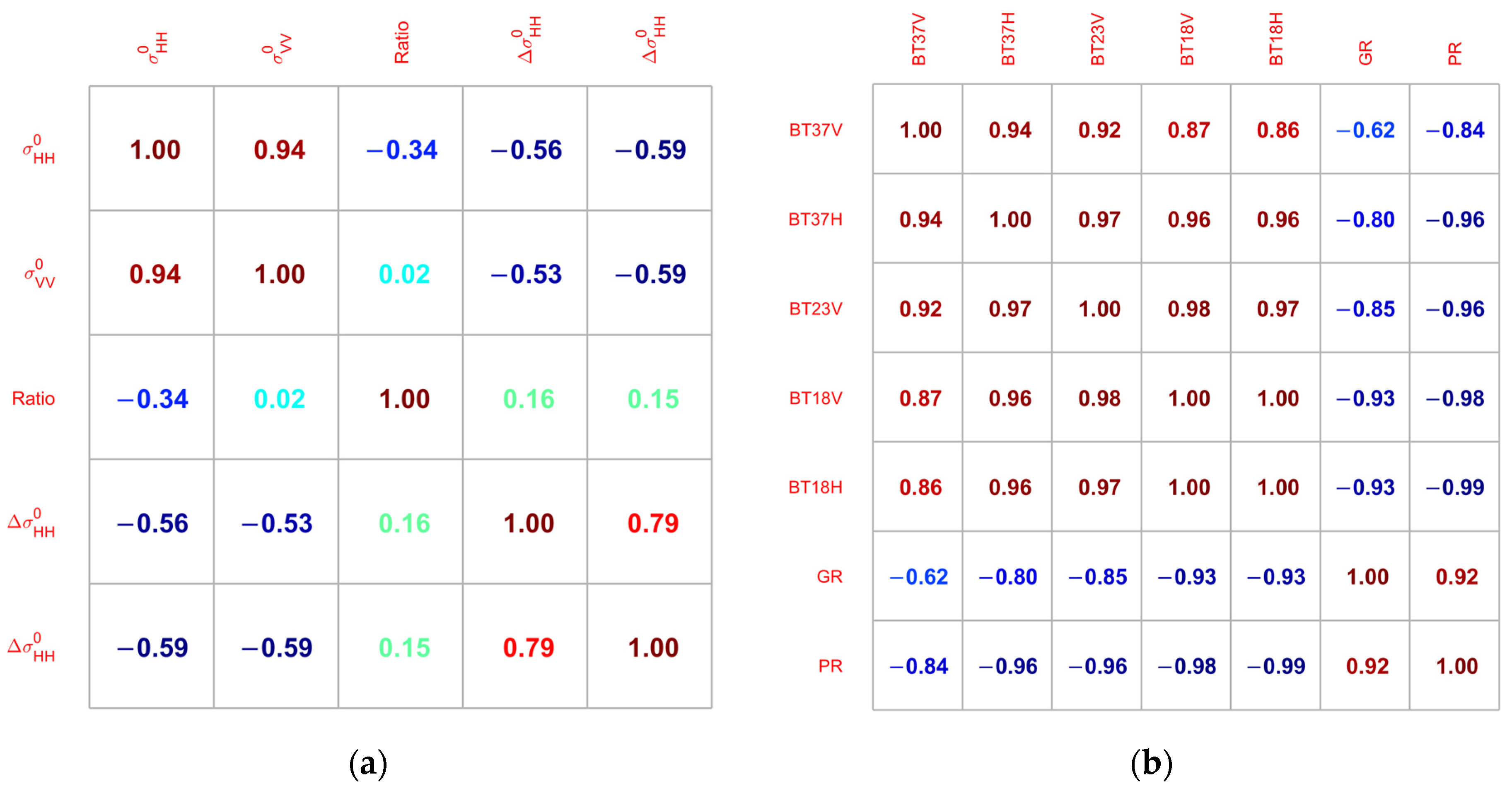
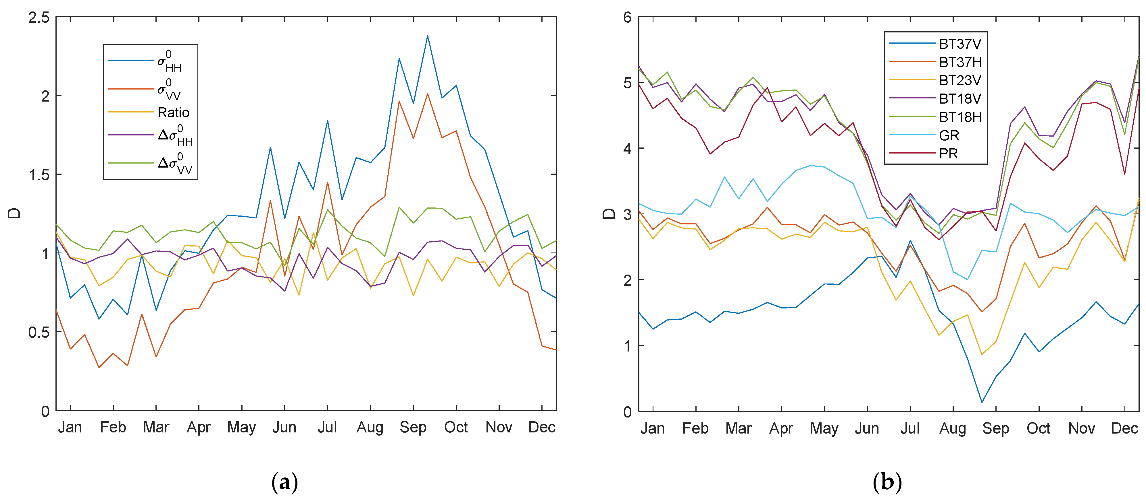
3.1. Microwave Radiation and Scattering Parameters and Selection Method

In addition to the two polarization modes backscattering coefficients of SCA, we also calculated three parameters, including the following:
1.
Polarization ratio, defined as the ratio of the horizontal polarization backscattering coefficient to the vertical backscattering coefficient:
ratio = σ HH 0 / σ VV 0
2.
Horizontal polarization standard deviation Δ σ HH 0 , defined as the standard deviation of multiple horizontal polarization observations in a single grid point.
3.
Vertical polarization standard deviation Δ σ VV 0 , defined as the standard deviation of multiple vertical polarization observations in a single grid point.
The observed microwave backscatter over sea ice is dependent on the various sea ice characteristics, such as surface roughness, liquid water content, covered snow and brine pockets. The snow cover and brine pocket distribution are related to sea ice age [34]. The σ VV 0 and σ HH 0 of ice are similar and the polarization ratio is close to 1. For the backscattering of sea water, the surface scattering is dominant and there is a large difference between σ VV 0 and σ HH 0 , so the polarization ratio is relatively high. The other two parameters were used to present the anisotropy of sea ice and water. The backscattering of sea ice is relatively isotropic and the calm open water is strongly anisotropic, so the Δ σ HH 0 and Δ σ VV 0 of calm water are larger than those of sea ice.
For the measurement of the SMR sensor, brightness temperatures of 6.9 GHz and 10.7 GHz were not used in this study because of their coarse spatial resolution. We selected the brightness temperature data of five bands at three observation frequencies of 18.7 GHz, 23.8 GHz and 37.0 GHz and calculated the polarization gradient ratio (PR) and spectral gradient ratio (GR). The calculation formula is given as follows:
PR   = T b , 18.7 V T b , 18.7 H / T b , 18.7 V + T b , 18.7 H
GR   = T b , 37 V T b , 18.7 V / T b , 37 V + T b , 18.7 V
These seven parameters are commonly used in algorithms to estimate ice concentration and distinguish between ice and water and different ice types [29].
There is a certain correlation between the above five scatterometer observation parameters and the seven radiometer observation parameters. Figure 3 shows the correlation coefficient of five SCA parameters and SMR’s seven parameters over the ocean area on 5 December 2019. The correlation between σ VV 0 and σ HH 0 is 0.94, the correlation between Δ σ VV 0 and Δ σ HH 0 is 0.79, and the ratio has a low correlation with the other four parameters. Figure 3b shows that the correlation between brightness temperature parameters is high, and the correlation between GR and PR is high; PR has a high negative correlation with the five brightness temperature parameters.
If the above 12 parameters are directly used to distinguish ice water and sea ice types, there will be a certain amount of data redundancy. With the amount of calculation increasing, the redundant bands will often interfere with the discrimination ability of other bands, and the accuracy of classification will be reduced. To solve this problem, we use the classification distance and correlation coefficient to select parameters. The classification distance is used to judge the classification ability of the ice water discrimination and sea ice type discrimination of different parameters. The formula below is the definition of the classification distance between ice and water. The definitions of the classification distances of FYI and MYI are similar.
D iw = μ i μ w σ i 2 + σ w 2
where μ i and μ w are the mean values of a certain parameter of sea ice and sea water samples, respectively. σ i 2 and σ w 2 are the variances in the corresponding parameters for the sea ice and sea water samples, respectively. A higher value of one parameter’s D iw means better ice water discrimination ability and is more suitable for sea ice information extraction. In contrast, a low value of D iw shows that the ice water discrimination ability of this parameter is relatively weak. At the same time, the correlation coefficient between different parameters is considered. If two or more parameters have similar values with classification distances and are highly correlated, only the parameter with the largest classification distance is selected for ice water discrimination.
Taking ice water discrimination over the Arctic as an example, we use the SIC data of NSIDC to establish sea ice marks with a 30% threshold. The pixels with an SIC greater than 30% are sea ice marks, and the pixels with an SIC of 0% are sea water marks. Based on the marks, the mean and variance in sea ice and sea water of a specific parameter are calculated, and then, the classification distance between ice and water for a certain parameter is calculated according to Formula (4). According to the calculation results, a group of parameters with large classification distances and weak correlations were selected for ice water discrimination.

3.2. Support Vector Machine (SVM) Method

The support vector machine (SVM) is a machine learning algorithm based on statistical theory [35]. It has been widely used in the field of remote sensing image classification. In this paper, the SVM method is used to establish a nonlinear ice/water classification model and Arctic FYI/MYI classification model. SVM makes data linearly separable by transferring low-dimensional vectors into high-dimensional space and introduces a kernel function to change the data into the desired form in high-dimensional space. For the two-class classification (ice/water and Arctic FYI/MYI) with the input data of SCA and SMR observation parameters, SVM finds an optimal classification hyperplane in high-dimensional space, which is recorded as w x + b = 0 , and transforms classification problems into constrained minimum value problems.
The optimal classification hyperplane satisfies the following maximum interval principle:
min‖w‖2/2
Constraints y i w x i + b 1   i = 1 , n
where w is the weight vector, x is the input characteristic parameter vector which is the parameter in Section 3.1 for distinguishing ice/water and FYI/MYI, x i is the ith component of vector x , and y is the classification mark. In known samples, sea ice is recorded as “2”, sea water is recorded as “1”, and y i is the ith component of vector y.
To consider the seasonal variation in sea ice microwave radiation and scattering characteristics, especially the variation in the sea ice melting period, as well as to improve the accuracy of ice water discrimination, we select 3 days (5th, 15th, and 25th) of data from each month in 2019 to establish a monthly SVM ice/water discrimination model and the amount of the sample data is more than 106. During the process of model establishment, we tried the 6 days data and 10 days data and the accuracy of the model was not obviously improved, but the training time of the model significantly increased. In the modeling process, the SIC data of NSIDC and the 30% threshold are used to establish the sea ice mark. For the FYI/MYI classification model, we selected [72~76°N, 158~177°E] and [75~80°N, 115~134°E] as the FYI characteristic area and [83~86°N, 120~150°W] as the MYI characteristic area [36]. Using the data of three days per month from January to April and October to December 2019, we established the monthly SVM sea ice type classification model. The statistics and machine learning toolbox of MATLAB were used to establish the above SVM modals [37] and to optimize the hyperparameters automatically using the fitcsvm function.

4. Results

In this section, we first selected suitable microwave radiation and scattering parameters for ice/water classification and sea ice type classification according to the classification distance and correlation coefficient. Then, the sea ice extent (SIE) and Integrated Ice Edge Error (IIEE) based on the ice/water classification in this study from 2019 to 2021 were compared with the other products. Finally, the results of the Arctic MYI extent were compared with similar OSISAF products.

4.1. Parameters Selection

We selected the observation data of 36 days on the 1st, 11th and 21st of each month in 2019 and calculated the ice/water classification distance for each parameter. Figure 4 shows the classification distances of the SCA’s five parameters and SMR’s seven parameters over the Arctic. The polarization ratio and the two standard deviations are relatively stable throughout the year, while the two backscattering coefficients show obvious seasonal changes. From June to October, the backscattering coefficient difference between the sea ice and the open water is more obvious due to the melting of sea ice, so the classification distances of σ VV 0 and σ HH 0 become large. Based on correlation matrix of Figure 3a, the five parameters of SCA can be classified into three categories: [ σ HH 0 ,   σ VV 0 ] , Ratio and [ Δ σ HH 0 ,   Δ σ VV 0 ] . Then, based on Figure 4a, the D value of σ HH 0 is higher than that of σ VV 0 , the D value of Δ σ VV 0 is higher than that of Δ σ HH 0 . Therefore, [ σ HH 0 ,   Ratio ,   Δ σ HH 0 ] was selected to distinguish ice from water. Similarly, the seven parameters of SMR can be classified into two categories: [ T b , 18.7 V ,   T b , 18.7 H , T b , 23.8 V , T b , 37 V , T b , 37 H ] and GR , PR . Then, based on Figure 4b, the D value of T b , 18.7 V is higher than that of other T b and the D value of PR is higher than that of GR. So, [ T b , 18.7 V ,   PR ] are selected from the seven parameters of SMR.
Through the above classification distance and correlation analysis, the parameters selected for the ice/water distinction of the Arctic and Antarctic are the same and given as follows: σ HH 0 ,   Ratio ,   Δ σ HH 0 , T b , 18.7 V ,     PR .
Figure 5 shows the sea ice extent over the Arctic on 5 March 2019, with the different input parameters and the product of OSISAF. Figure 5a is the result of five SCA parameters, Figure 5b is the result of three SCA parameters σ HH 0 ,   Ratio ,   STD H and Figure 5c is the result of σ HH 0 ,   Ratio ,   STD H ,   T b , 18.7 V ,   PR . Using the OSISAF result as the standard, the results based on the SCA parameters (Figure 5a,b) have some incorrect identifications of ice and water over the area within the red frame (Beaufort Sea, northern part of Okhotsk Sea, Hudson Bay and Baltic Sea), and this problem is solved by introducing two radiometer parameters. The results of the Daily Arctic Marginal Ice Zone (MIZ) chart and Interactive Multisensor Snow and Ice Mapping System (IMS) released by the National Ice Center (NIC) are consistent with the sea ice extents of Figure 5c,d, especially over the above four areas. Compared with using the SCA data alone, the accuracy of ice water discrimination was increased by combining the SCA data and SMR data.
Figure 5 only shows the results of one day. Using the OSISAF product as a reference, the overall accuracy (OA) and Kappa coefficient of the result with five SCA parameters and the result with selected parameters of SCA and SMR over the Arctic and Antarctic from 2019 to 2021 were calculated and are shown in Figure 6. The OA and the Kappa coefficient of the SCA and SMR results is higher than those parameters of the SCA result. For the Arctic results of the SCA and SMR, the three-year averaged OA is 0.9904 and the Kappa coefficient is 0.9681, better than 0.9848 and 0.9497, respectively, of the five SCA parameters. For the Antarctic result of SCA and SMR, the averaged OA is 0.9915 and the Kappa coefficient is 0.9631, better than 0.9818 and 0.9255, respectively, of the five SCA parameters. So, the combination of the SCA and SMR observation has less difference with OSISAF products than only using SCA observation.
The classification distance of FYI/MYI with 12 parameters in Section 3.1 was calculated; then, the same parameters selection method for the ice water discrimination were used and σ HH 0 ,   T b , 18.7 H ,   PR were selected as the input parameters for FYI/MYI classification.

4.2. Comparison of Sea Ice Extent and IIEE over the Arctic and Antarctic

Based on the results of ice water identification in this paper, the Arctic and Antarctic sea ice extents from 2019 to 2021 are calculated and compared with the results of other products, including the sea ice extent calculated using NSIDC’s SIC product with 15% and 30% thresholds, respectively, and the sea ice extent is calculated using OSISAF sea ice edge products. Considering the different spatial resolutions, each pixel area of the first three sea ice extents is 625 km2 and each pixel area of OSISAF is 100 km2. Figure 7 shows the comparison results of the four sea ice extents. The seasonal variation trend of the four time series products is consistent. The sea ice extent result obtained using HY-2B fluctuated between NSIDC 15% and NSIDC 30%. The results of OSISAF are lower than those of the other three sea ice extents, especially in the Arctic, because the land mass used by OSISAF is larger than that of the other three products and the sea ice around the land of OSISAF is not included in the sea ice extent calculation. Table 2 lists the sea ice extent difference between HY-2B and the other three products in Figure 7. The difference between HY-2B and NSIDC 15% is the smallest, and the difference between the Antarctic and the Arctic is −0.16 ± 0.13 × 10⁶ km2 and −0.19 ± 0.14 × 10⁶ km2, respectively. The difference between HY-2B and OSISAF is the largest, especially in the Arctic, with a value of 1.76 ± 0.77 × 10⁶ km2. Based on the 3-year daily sea ice extents in Figure 7, we also compared the seasonal mean values and standard deviations of different products. All products have relatively large standard deviations in the summer and autumn periods (from July to September) and small standard deviations in the winter and spring periods (from October to May). For example, over the Arctic, the mean value and standard deviation of HY-2B in the summer of 2019 was 7.32 ± 2.38 × 10⁶ km2, while the mean value and standard deviation of HY-2B in the winter of 2019 was 13.24 ± 1.31 × 10⁶ km2. Similarly to the daily comparison results, the seasonal mean value of HY-2B has better agreement with NSIDC 15% than that of NSIDC 30% and OSISAF.
The above sea ice extent cannot present the spatial similarity of the two sea ice edges of different products. The IIEE was used to evaluate the spatial disagreement of sea ice edges between HY-2B and other products [38,39]. For example, the IIEE between HY-2B and NSIDC was defined as the sea ice extent sum of the area that was covered by the HY-2B result, but not covered by NSIDC’s SIC product with 15% thresholds, and the area that was not covered by the HY-2B result, but covered by NSIDC’s SIC product with 15% thresholds. Figure 8 shows the time series of IIEE between HY-2B and other products over the Arctic and Antarctic from 2019 to 2021. For the Arctic, the IIEEs do not present the seasonal variation. The mean value and standard deviation (STD) of IIEE between HY-2B and NSIDC is 1.03 ± 0.12 × 10⁶ km2, and the mean value and STD of IIEE between HY-2B and OSISAF is 0.40 ± 0.12 × 10⁶ km2. For the Antarctic, the IIEEs show the seasonal variation and high values during the sea ice melting season. The mean value and STD of IIEE between HY-2B and NSIDC is 0.83 ± 0.21 × 10⁶ km2, and the mean value and STD of IIEE between HY-2B and OSISAF is 0.44 ± 0.20 × 10⁶ km2. The above results mean that the sea ice edge of HY-2B is closer to the sea ice edge of OSISAF than that of NSIDC. A possible reason is that the OSISAF product is also based on observation data from scatterometers (ASCAT) and microwave radiometers (SSMIS), similarly to this study. Therefore, in the next section, the accuracy of HY-2B ice water discrimination will be evaluated based on OSISAF.

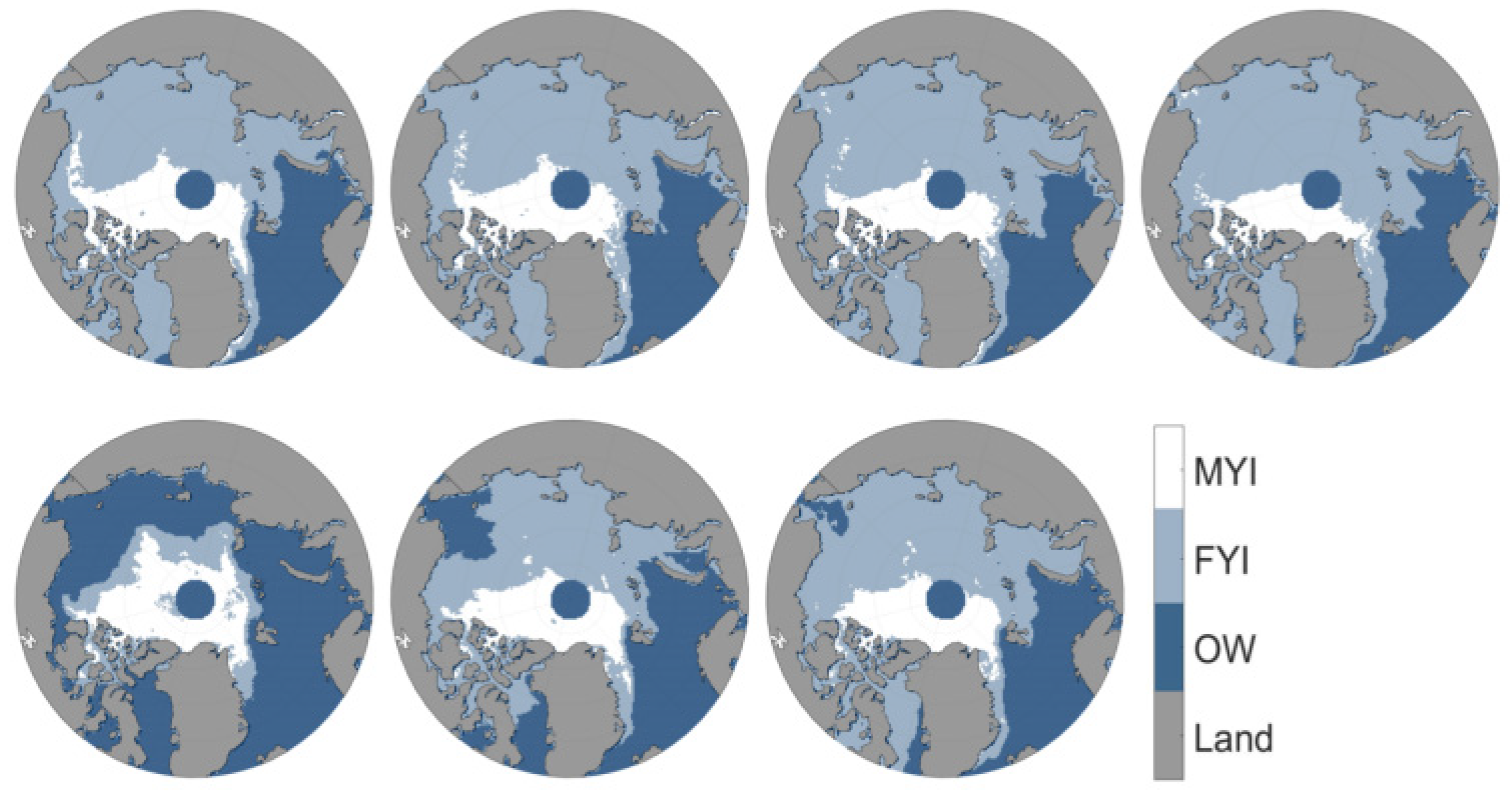
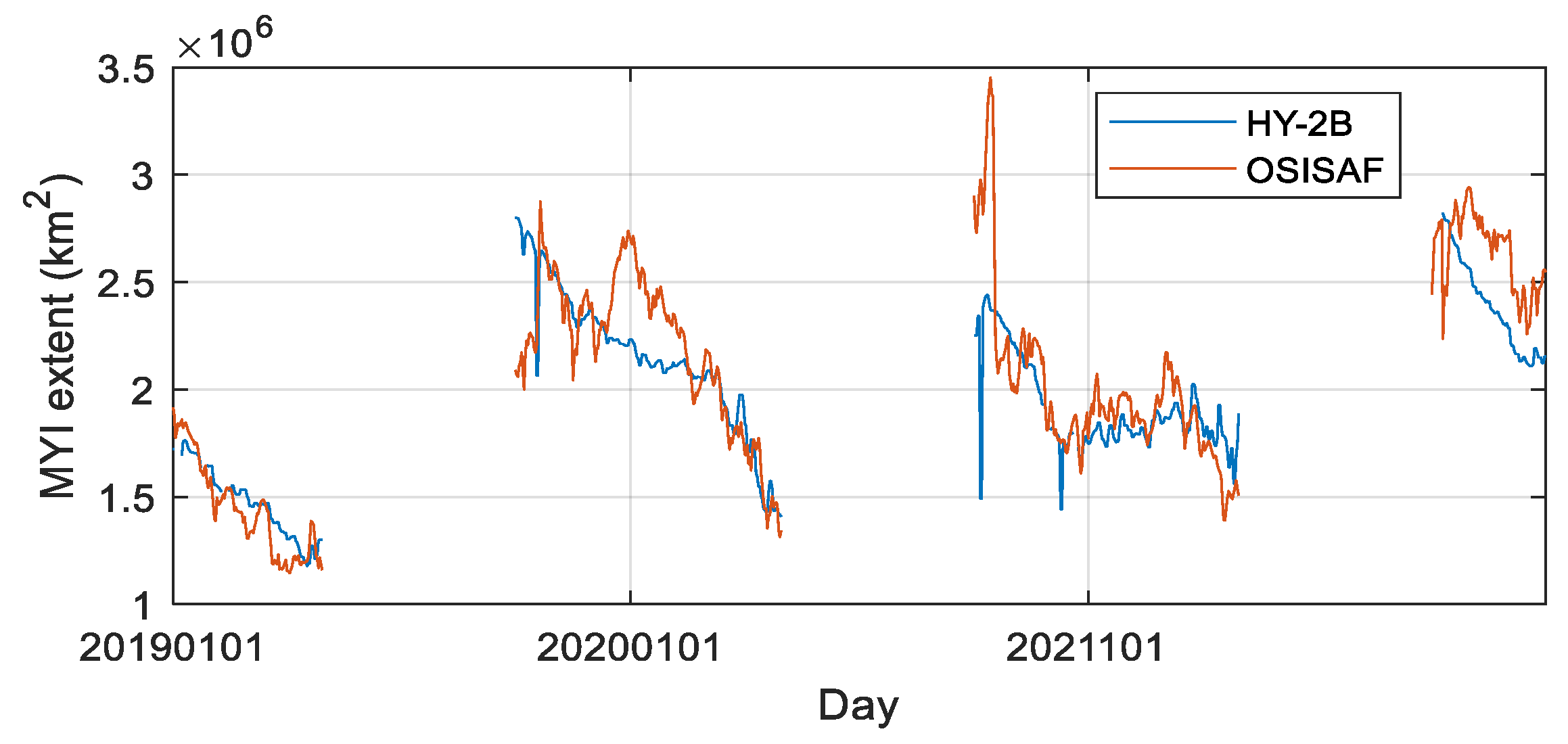
4.3. Arctic Sea Ice Type Results

Using σ HH 0 ,   T b , 18.7 H ,   PR as the input parameter of the monthly SVM sea ice type discrimination model, we calculated the classification results of FYI/MYI over the Arctic from January to April and from October to December of 2019–2021. Figure 9 shows the classification results of Arctic sea ice from January to April and October to December 2019.
Since there are no observations using SCA over the central area of the Arctic, there is a circular area with missing data in the sea ice classification results. Most MYI is distributed over the northern part of Canada and Greenland. The MYI gradually decreased from January to April, and the extent of MYI reached a maximum in October, which extended to the mid-Arctic region and then gradually decreased. Figure 10 shows the comparison between the MYI extent in this paper and the OSISAF results from 2019 to 2021. The seasonal variation trends of the two results are generally consistent, and there are three abrupt values in the HY-2B results, mainly due to the lack of data on that day. In the two time periods from December 2019 to February 2020 and from October to December 2021, the results of OSISAF are significantly higher than those of HY-2B, which is the difference in MYI over the central Arctic. OSISAF’s result fluctuates more than HY-2B, which is similar with the result of Zhang et al. [8]. The main reason could be that the Ku band SCA observation of HY-2B is more sensitive to the MYI/FYI discrimination than the C band ASCAT observation used in the OSISAF product [8].

5. Assessment

To quantitatively assess the result of HY-2B, this section presents the general evaluation with the OSISAF similar product and the detailed pixel-based evaluation with MODIS and SAR images.

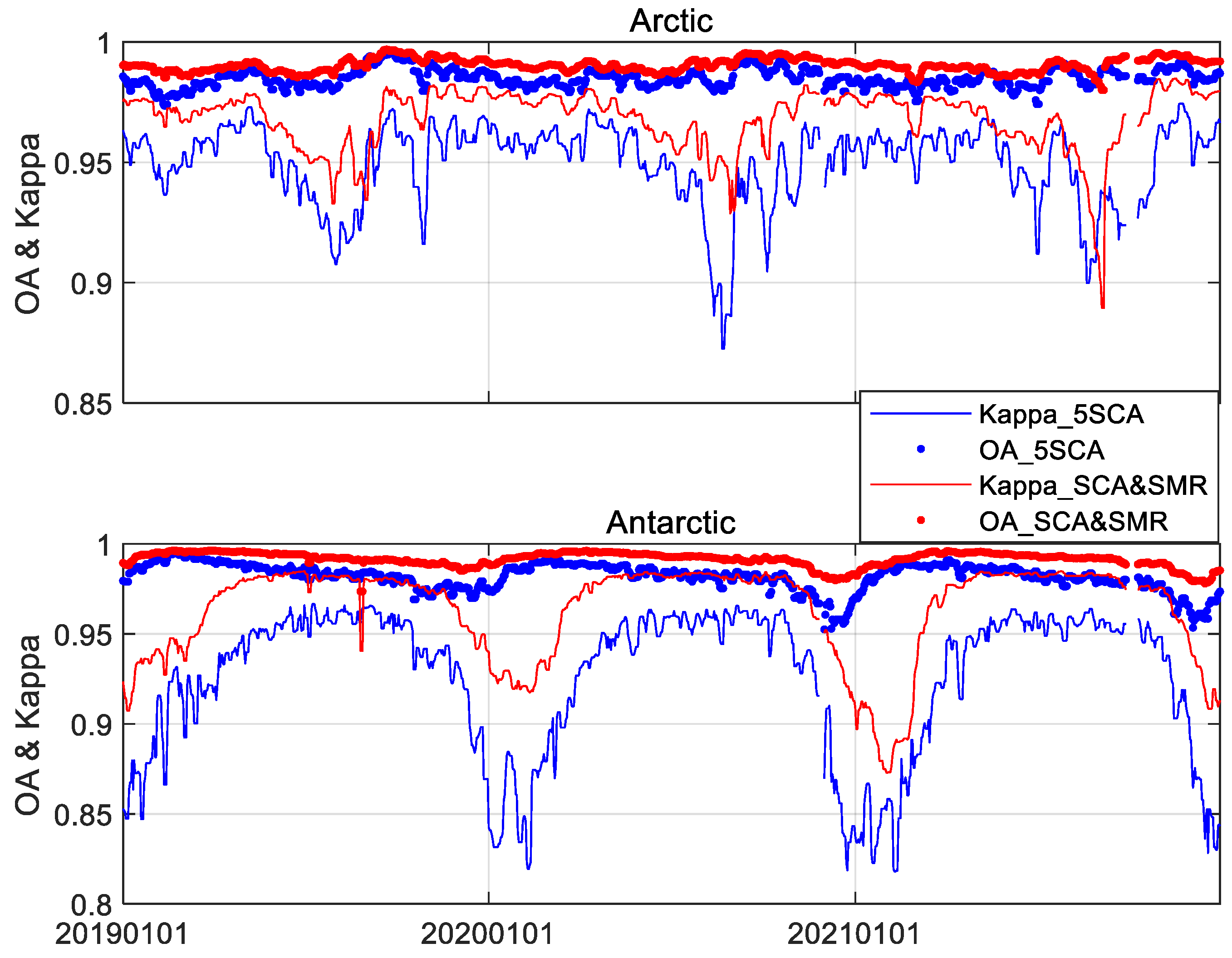
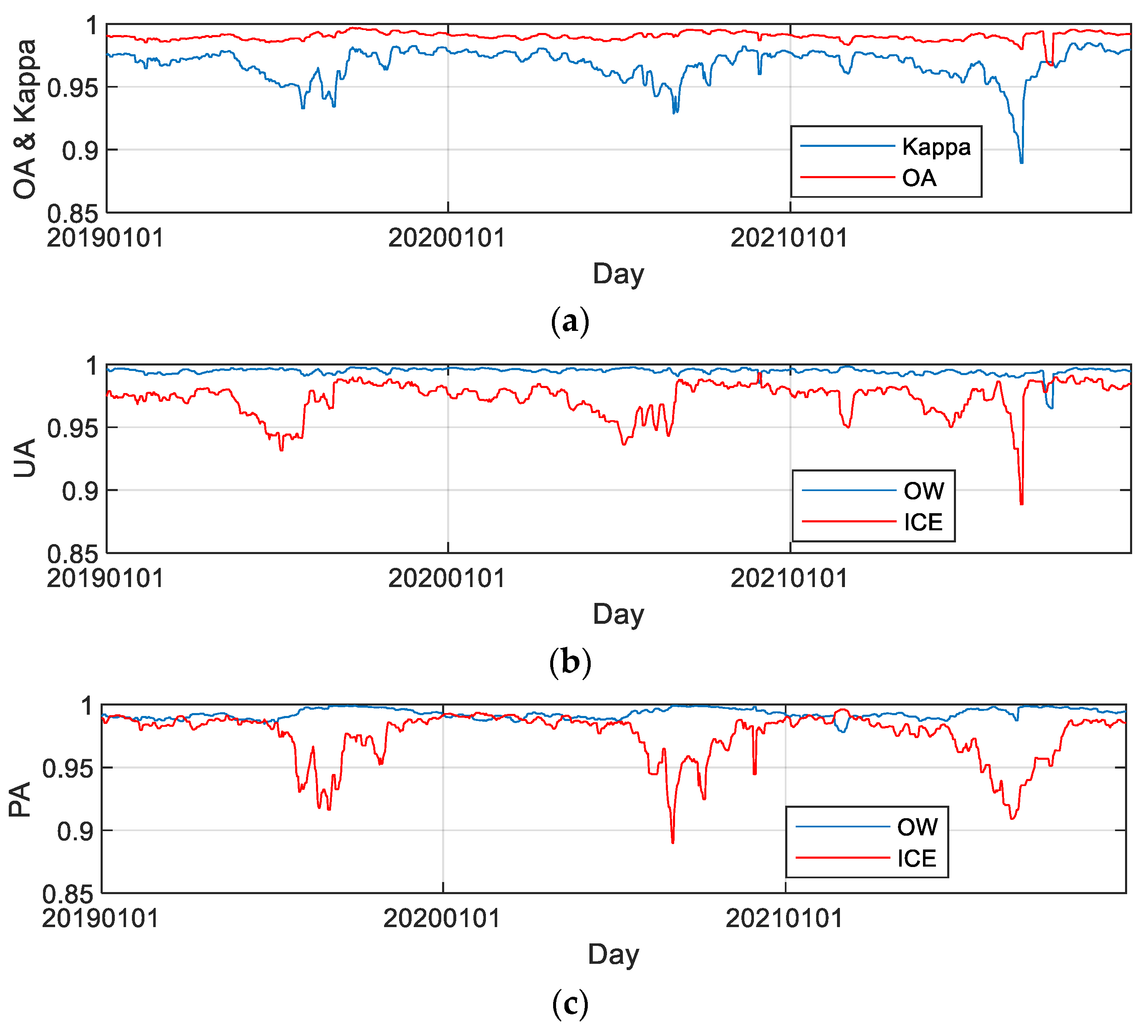
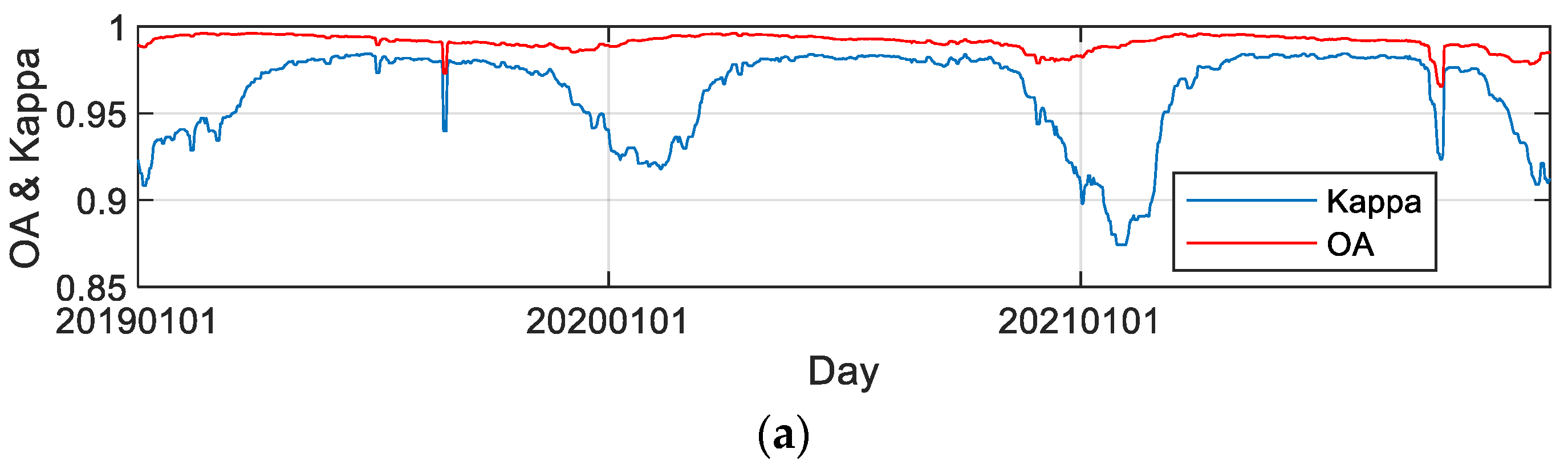
5.1. Assessment of Ice Water Discrimination Results with OSISAF Ice Edge Product

Using the sea ice edge product of OSISAF over the Arctic and Antarctic as the reference data, the ice water discrimination result of HY-2B is quantitatively assessed with the specific evaluation parameters derived from the confusion matrix, including overall accuracy (OA), Kappa coefficient (Kappa), producer’s accuracy (PA) and user’s accuracy (UA). Figure 11 and Figure 12 show the time series of the above evaluation parameters in the Arctic and Antarctic from 2019 to 2021, respectively, the averaged classification accuracies of which are summarized in Table 3. It should be noted that the sea ice edge product of OSISAF includes the classes of OW and the open sea ice and closed sea ice are merged into ice and compared with the results of HY-2B.
For the Arctic and Antarctic, the averaged values of OA, UA_OW and PA_OW are higher than 99% and show no obvious seasonal variation. The averaged values of Kappa, UA_Ice and PA_Ice are relatively low and the time series of these three parameters show obvious seasonal changes. For the Arctic, Kappa and UA_Ice decreased significantly in late May, while PA_Ice began to decrease in July. At the beginning of the melting season, some OW pixels of the OSISAF product were classified as ice in the HY-2B result. With increasing temperature, ice surface melting intensified, and some ice pixels of OSISAF were classified as OW in the HY-2B result. The seasonal variations in Kappa, UA_Ice and PA_Ice in Antarctica are similar to those in the Arctic, Kappa and UA_Ice decreased significantly in December and PA_Ice began to decrease in January.
For the results of Arctic or Antarctic, the decline date of PA_Ice is approximately one month delayed compared to that of Kappa and UA_Ice. The possible reasons are as follows. First, HY-2B’s ice water identification model in this paper is a monthly model, while the Bayesian method of OSISAF products uses a 15-day moving average PDF. The model in this paper does not present the changes in backscattering and radiation caused by sea ice melting. Second, the Ku band SCA data in this paper and C band ASCAT data in the OSISAF product have different OW/Ice discrimination abilities because of the different observation bands and the different observation geometries of the two sensors. In the ice melting period, with the melting of snow on the ice surface and the presence of melting pools, the accuracy of ice water identification is much lower than that in the sea freezing period.

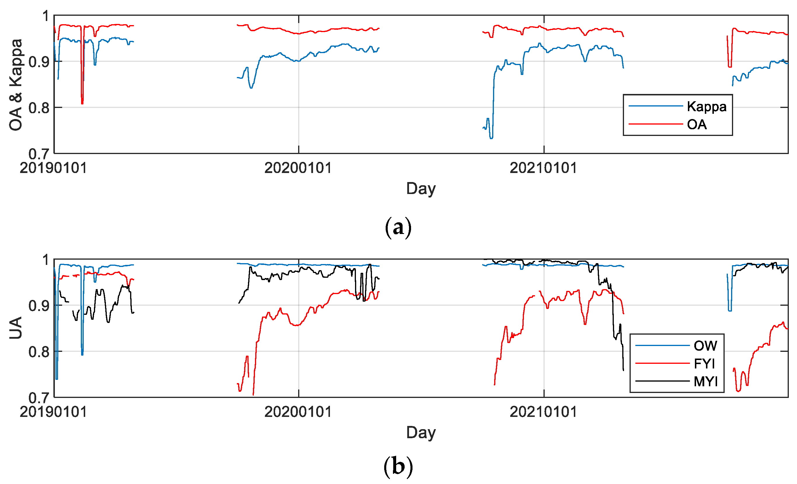
5.2. Assessment of Ice-Type Discrimination Results with OSISAF Ice-Type Product

Using the sea ice type product of OSISAF as reference data, the ice-type discrimination result of HY-2B is quantitatively assessed with the parameters derived from the confusion matrix. Figure 13 shows the time series of the evaluation parameters in the Arctic from 2019 to 2021. The large dip of a certain day’s parameters is caused by the missing data of HY-2B. The average OA and Kappa are 96.82% and 0.837, respectively, which are much lower than the ice water discrimination results. The averaged UAs of OW, FYI and MYI are 98.32%, 88.11% and 94.78%, respectively, and the averaged PAs of OW, FYI and MYI are 99.35%, 93.94% and 67.50%, respectively. The UA_FYI and PA_MYI are much lower than other parameters. Compared with the OSISAF result, some MYI is misclassified as FYI in the HY-2B result.

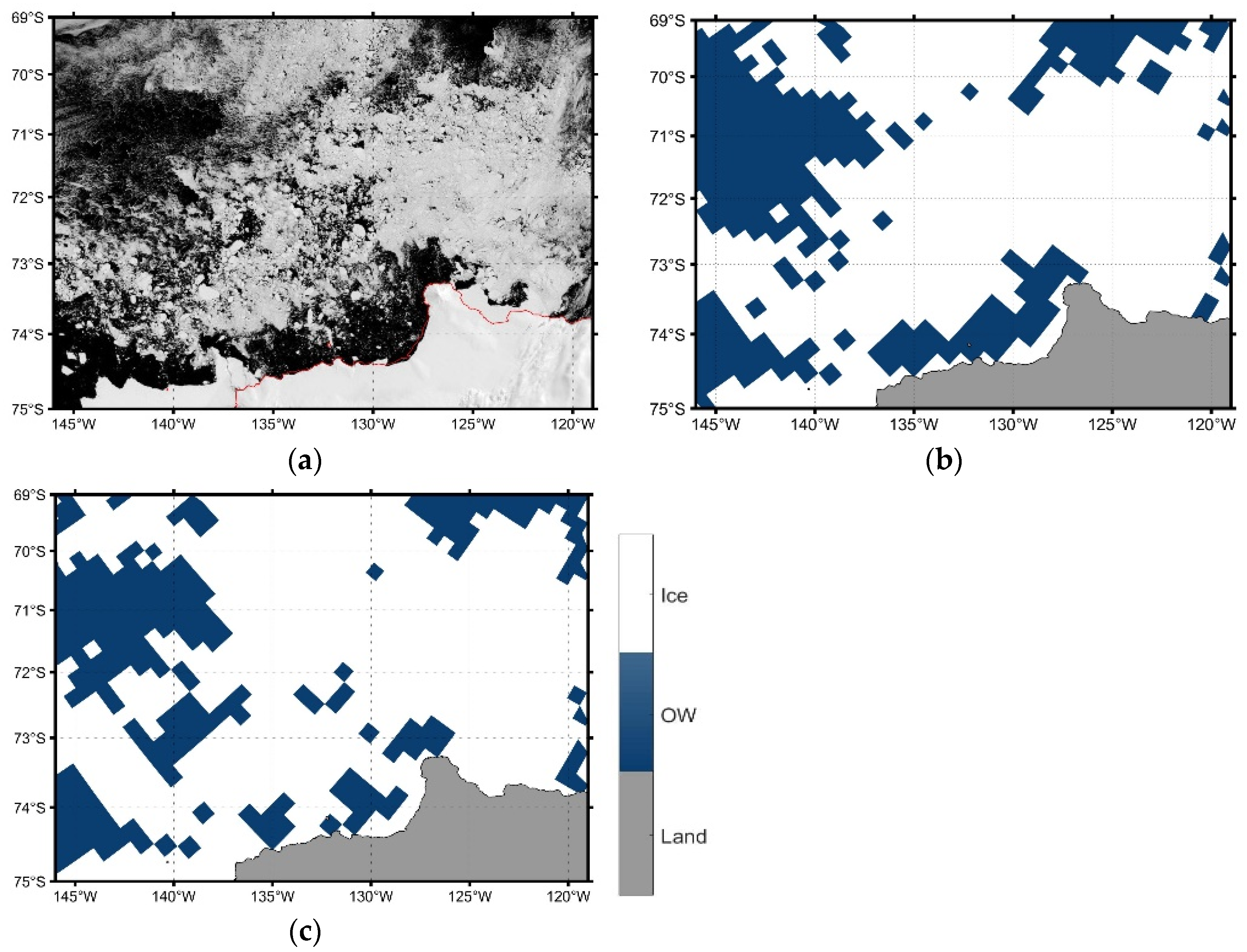
5.3. Assessment of Ice Water Discrimination Results with MODIS Images

Based on the cloud-free MODIS optical image with a resolution of 1 km, ice can be distinguished from water according to the difference in ice water reflectivity. Figure 14 shows the comparison of MODIS images and sea ice distribution near the Canadian Archipelago on 1 July 2019. Figure 14a shows the MODIS image; the red line is the coastline. The sea water reflectivity is low, and the sea ice reflectivity is high, which makes it easier to distinguish the ice area. The ocean areas in the MODIS images were classified into FYI and OW with the ISODATA unsupervised classification method and were revised by visual interpretation. Then, the proportion of sea ice pixels in each 25 km × 25 km grid was calculated based on the ice water discrimination results. Using 30% as the threshold, the sea ice extent results with a 25 km spatial resolution (Figure 14b) were obtained. Comparing the results with the same regional results of HY-2B (Figure 14c), the spatial distribution of the MODIS results is consistent with that of the HY-2B results, and the long and narrow polynya on the upper left side of the image is also presented in the HY-2B results. The spatial solution of the HY-2B result needs to be improved in a future study. The OSISAF product is more consistent with the MODIS result because of its higher spatial resolution with 10 km. To carry out quantitative evaluation, we calculated the confusion matrix between the HY-2B results and MODIS results. As shown in Table 4, the OA is 91.04%, and the Kappa coefficient is 0.736, which shows that the overall consistency of the two results is high. The PA and UA of seawater are relatively low, which is mainly due to the difference between the two results in the ice water junction area and is caused by the spatial resolution and observation time difference between HY-2B and MODIS. The spatial resolution of HY-2B is much coarser than that of MODIS; for example, the OW with a narrow and long shape in the upper left part of Figure 14a is only partially presented as OW in the results of HY-2B. The HY-2B product is a daily averaged observation, while MODIS data are at a specific time, so the sea ice edge regions with drastic changes present great differences between the HY-2B and MODIS results.
Figure 15 shows the comparison of MODIS images and sea ice distribution near the Ross Sea on 2 January 2020. Table 5 shows the confusion matrix between the corresponding HY-2B result and MODIS result, with an overall accuracy of 87.00% and Kappa coefficient of 0.680. The UA of seawater is low (70.29%), which indicates that the pixels identified as seawater in the HY-2B result are classified as sea ice in the MODIS result. In this case, the OW area over the left part and lower middle part of the MODIS image is classified as sea ice in the HY-2B result. This difference is caused by the observation time difference between HY-2B and MODIS in the last case.

5.4. Assessment of Ice-Type Discrimination Results with SAR Images

According to the reflectivity difference between ice and water, the extraction of sea ice extent can be realized by using MODIS optical images, but it is difficult to distinguish MYI from FYI. However, due to the difference in surface roughness and volume scattering between FYI and MYI, SAR images can be used to distinguish sea ice types and obtain the results of sea ice types with high spatial resolution. Figure 16 shows the SAR image of the HH polarization band and FYI/MYI distribution near the Canadian Archipelago on 18 January 2019. In the SAR image, the upper right part and some areas between islands with low backscattering coefficients are covered by FYI, and the remainders with high backscattering coefficients are covered by MYI. Using the ISODATA unsupervised classification method and visual interpretation [8,22], FYI and MYI were distinguished and are shown in Figure 16b. MYI is shown in white, FYI is shown in light blue, and the area without observations is shown in dark blue. The spatial distributions of the SAR and HY-2B sea ice types (Figure 16c) are roughly consistent. In the lower right area, it was recognized as MYI in the SAR result, but it was recognized as FYI in the HY-2B result. To reduce the SAR result’s spatial resolution to 25 km, the proportions of FYI and MYI pixels in each 25 km × 25 km grid of Figure 16b are calculated based on Figure 16b. Then, for each grid, the proportions of FYI and MYI are compared and the sea ice type corresponding to the larger proportion is determined. Finally, the sea ice type results with a 25 km spatial resolution are compared with the result of HY-2B (Figure 16c) over the same area and the confusion matrix is shown in Table 6. The overall accuracy is 86.82%, the Kappa coefficient is 0.733, and the PA and UA results are greater than 80%.
Figure 17 shows the SAR image and FYI/MYI distribution near the Canadian islands on 23 December 2019. Table 7 shows the confusion matrix between the HY-2B and SAR sea ice type recognition results. The overall accuracy is 88.48%, the Kappa coefficient is 0.755, and the PA and UA results are greater than 85%. Compared with the assessment results of ice water identification, the evaluation accuracy of sea ice type identification is relatively low, which is mainly because the spatial resolution of the data used in this study is 25 km, so it is difficult to give accurate results in the area of MYI and FYI fusion.

6. Conclusions

In this study, using the active microwave scatterometer and passive microwave scanning radiometer observations of the HY-2B satellite, a monthly polar ice water discrimination model and Arctic sea ice type classification model based on the SVM method were established, and the sea ice extent products and sea ice type products from 2019 to 2021 were calculated. The results of this study were evaluated with NSIDC, OSISAF, MODIS and SAR data. The main conclusions are given as follows:
(1)
In this study, the classification distance and correlation coefficient were used to select the scattering parameters of SCA and the microwave radiation parameters of SMR suitable for ice water discrimination and sea ice type discrimination, which reduces the redundancy of the input data. At the same time, including SMR brightness temperature data can obtain better ice water discrimination results than SCA data alone. The sea ice extent results obtained using HY-2B products are between NSIDC 15% and NSIDC 30%, and the result of OSISAF is lower than those of the other three sea ice extents. The sea ice extent difference between HY-2B and NSIDC 15% is the smallest. The IIEE evaluation results show that the sea ice edge of HY-2B is closer to the sea ice edge of OSISAF than that of NSIDC. Using 3 years of the OSISAF sea ice edge product as reference data, the averaged OA of the HY-2B ice water discrimination results of the Arctic and Antarctic is better than 99%. Compared with the results of MODIS ice water recognition, the overall accuracy is up to 96%.
(2)
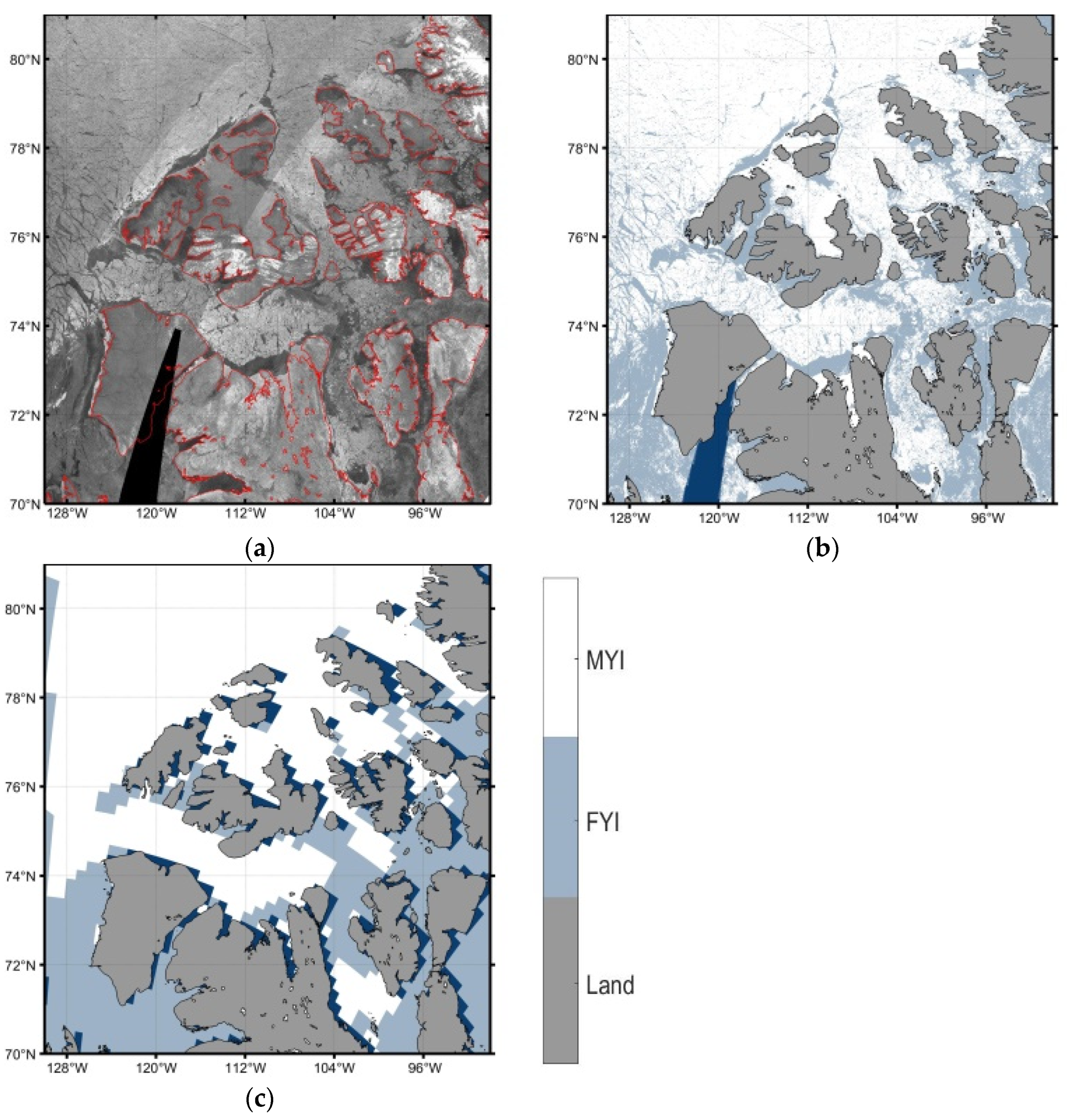
The results of the Arctic MYI extent agree with the OSISAF sea ice type products. Using the 3-year OSISAF product as the reference data, the OA of the HY-2B sea ice type results is approximately 97%. Using the results of SAR sea ice type recognition to evaluate the same results of this study, the overall accuracy is better than 86%. The recognition method of FYI/MYI needs to be further studied to improve the stability and classification accuracy. The detailed comparison of sea ice type classification results over some local areas, e.g., the north marine area of Greenland, will be analyzed with long time-series products of HY-2B and OSISAF.
This research assessed the HY-2B’s SCA and SMR performance of sea ice extent and sea ice type detection for the first time and laid the foundation for polar sea ice monitoring using similar data from existing and subsequent HY-2 series satellites. HY-2B is able to be one of the earth observation data sources for the long time-series of polar sea ice products. The existing 25 km resolution products cannot meet the needs of some local applications and a higher spatial resolution product can be achieved with an image reconstruction method or through combining with SAR data in the future.

Author Contributions

Data curation and writing, T.Z. and L.S.; methodology, L.S.; validation, Y.S. and D.L.; supervision and funding acquisition, Q.W. All authors have read and agreed to the published version of the manuscript.

Funding

This research was funded by the National Key Research and Development Program of China under Grant 2022YFC2807003) and the Impact and Response of Antarctic Seas to Climate Change program (grant number IRASCC2020-2022-No. 01-01-03).

Data Availability Statement

Data available in a publicly accessible repository that does not issue DOIs: Publicly available datasets were analyzed in this study. This data can be found here: ftp://ftp2.nsoas.org.cn (accessed on 1 July 2024).

Acknowledgments

The authors would like to thank NSIDC for providing the SIC data, the OSISAF for providing the sea ice edge and sea ice type data, the NASA for providing the MODIS imageries, and the DTU for providing the SAR mosaic imageries.

Conflicts of Interest

The authors declare no conflicts of interest.

References

  1. Meredith, M.; Cassotta, S. Polar Regions. In IPCC Special Report on the Ocean and Cryosphere in a Changing Climate; Pörtner, H.-O., Roberts, D.C., Masson-Delmotte, V., Zhai, P., Tignor, M., Poloczanska, E., Mintenbeck, K., Alegría, A., Nicolai, M., Okem, A., et al., Eds.; Cambridge University Press: Cambridge, UK, 2022; pp. 203–320. [Google Scholar]
  2. Comiso, J.C.; Meier, W.N.; Gersten, R. Variability and trends in the Arctic Sea ice cover: Results from different techniques. J. Geophys. Res. Oceans 2017, 122, 6883–6900. [Google Scholar] [CrossRef]
  3. Onarheim, I.H.; Eldevik, T.; Smedsrud, L.H.; Stroeve, J.C. Seasonal and Regional Manifestation of Arctic Sea Ice Loss. J. Clim. 2018, 31, 4917–4932. [Google Scholar] [CrossRef]
  4. Ludescher, J.; Yuan, N.; Bunde, A. Detecting the statistical significance of the trends in the Antarctic sea ice extent: An indication for a turning point. Clim. Dyn. 2019, 53, 237–244. [Google Scholar] [CrossRef]
  5. Turner, J.; Phillips, T.; Marshall, G.J.; Hosking, J.S.; Pope, J.O.; Bracegirdle, T.J.; Deb, P. Unprecedented springtime retreat of Antarctic sea ice in 2016. Geophys. Res. Lett. 2017, 44, 6868–6875. [Google Scholar] [CrossRef]
  6. Kusahara, K.; Reid, P.; Williams, G.D.; Massom, R.; Hasumi, H. An ocean-sea ice model study of the unprecedented Antarctic sea ice minimum in 2016. Environ. Res. Lett. 2018, 13, 084020. [Google Scholar] [CrossRef]
  7. Rivas, M.B.; Otosaka, I.; Stoffelen, A.; Verhoef, A. A scatterometer record of sea ice extents and backscatter: 1992–2016. Cryosphere 2018, 12, 2941–2953. [Google Scholar] [CrossRef]
  8. Zhang, Z.; Yu, Y.; Li, X.; Hui, F.; Cheng, X.; Chen, Z. Arctic sea ice classification using microwave scatterometer and radiometer data during 2002–2017. IEEE Trans. Geosci. Remote Sens. 2019, 57, 5319–5328. [Google Scholar] [CrossRef]
  9. Onstott, R.G. SAR and Scatterometer Signatures of Sea Ice. In Microwave Remote Sensing of Sea Ice; Geophysical Monograph Series; American Geophysical Union: Washington, DC, USA, 1992; pp. 73–104. [Google Scholar] [CrossRef]
  10. Sinha, N.K.; Shokr, M. Sea Ice: Physics and Remote Sensing, 1st ed.; John Wiley & Sons: Hoboken, NJ, USA, 2015; pp. 412–424. [Google Scholar]
  11. Remund, Q.; Long, D. Automated Antarctic ice edge detection using NSCAT data. IGARSS′97. In Proceedings of the 1997 IEEE International Geoscience and Remote Sensing, Remote Sensing—A Scientific Vision for Sustainable Development, Singapore, 3–8 August 1997; pp. 1841–1843. [Google Scholar]
  12. Remund, Q.P.; Long, D.G. Sea ice extent mapping using Ku band scatterometer data. J. Geophys. Res. Oceans 1999, 104, 11515–11527. [Google Scholar] [CrossRef]
  13. Otosaka, I.; Rivas, M.B.; Stoffelen, A. bayesian sea ice detection with the ERS scatterometer and sea ice backscatter model at C-band. IEEE Trans. Geosci. Remote Sens. 2018, 56, 2248–2254. [Google Scholar] [CrossRef]
  14. Rivas, M.B.; Stoffelen, A. New bayesian algorithm for sea ice detection with QuikSCAT. IEEE Trans. Geosci. Remote Sens. 2011, 49, 1894–1901. [Google Scholar] [CrossRef]
  15. Rivas, M.B.; Verspeek, J.; Verhoef, A.; Stoffelen, A. Bayesian sea ice detection with the advanced scatterometer ASCAT. IEEE Trans. Geosci. Remote Sens. 2012, 50, 2649–2657. [Google Scholar] [CrossRef]
  16. Li, M.; Zhao, C.; Zhao, Y.; Wang, Z.; Shi, L. Polar sea ice monitoring using HY-2A scatterometer measurements. Remote Sens. 2016, 8, 688. [Google Scholar] [CrossRef]
  17. Shi, L.; Li, M.; Zhao, C.; Wang, Z.; Shi, Y.; Zou, J.; Zeng, T. Sea ice extent retrieval with HY-2A scatterometer data and its assessment. Acta Oceanol. Sin. 2017, 36, 76–83. [Google Scholar] [CrossRef]
  18. Brath, M.; Kern, S.; Stammer, D. Sea ice classification during freeze-up conditions with multifrequency scatterometer data. IEEE Trans. Geosci. Remote Sens. 2013, 51, 3336–3353. [Google Scholar] [CrossRef]
  19. Swan, A.M.; Long, D.G. Multiyear arctic sea ice classification using QuikSCAT. IEEE Trans. Geosci. Remote Sens. 2012, 50, 3317–3326. [Google Scholar] [CrossRef]
  20. Lindell, D.B.; Long, D.G. Multiyear Arctic sea ice classification using OSCAT and QuikSCAT. IEEE Trans. Geosci. Remote Sens. 2016, 54, 167–175. [Google Scholar] [CrossRef]
  21. Lindell, D.B.; Long, D.G. Multiyear Arctic ice classification using ASCAT and SSMIS. Remote Sens. 2016, 8, 294. [Google Scholar] [CrossRef]
  22. Zhang, Z.; Yu, Y.; Shokr, M.; Li, X.; Ye, Y.; Cheng, X.; Chen, Z.; Hui, F. Intercomparison of Arctic sea ice backscatter and ice type classification using Ku-band and C-band scatterometers. IEEE Trans. Geosci. Remote Sens. 2021, 60, 4301718. [Google Scholar] [CrossRef]
  23. Nghiem, S.; Rigor, I.; Clemente-Colón, P.; Neumann, G.; Li, P. Geophysical constraints on the Antarctic sea ice cover. Remote Sens. Environ. 2016, 181, 281–292. [Google Scholar] [CrossRef]
  24. Jia, Y.; Yang, J.; Lin, M.; Zhang, Y.; Ma, C.; Fan, C. Global assessments of the HY-2B measurements and cross-calibrations with Jason-3. Remote Sens. 2020, 12, 2470. [Google Scholar] [CrossRef]
  25. HY-2B. Available online: http://www.nsoas.org.cn/news/content/2018-11/23/44_697.html (accessed on 1 February 2022).
  26. Pearson, F. Map Projections: Theory and Applications; CRC Press: Boca Raton, FL, USA, 1990. [Google Scholar]
  27. Snyder, J.P. Map Projections—A Working Manual; US Government Printing Office: Washington, DC, USA, 1987. [Google Scholar]
  28. Nghiem, S.; Bertoia, C. Study of Multi-Polarization C-Band Backscatter Signatures for Arctic Sea Ice Mapping with Future Satellite SAR. Can. J. Remote Sens. 2001, 27, 387–402. [Google Scholar] [CrossRef]
  29. Cavalieri, D.J.; Parkinson, C.L.; Gloersen, P.; Zwally, H.J. Sea Ice Concentrations from Nimbus-7 SMMR and DMSP SSM/I-SSMIS Passive Microwave Data, Version 1; NASA National Snow and Ice Data Center Distributed Active Archive Center: Boulder, CO, USA, 1996. [Google Scholar]
  30. Global Sea Ice Edge. Available online: https://osi-saf.eumetsat.int/products/osi-402-d (accessed on 10 May 2022).
  31. Global Sea Ice Type. Available online: https://osi-saf.eumetsat.int/products/osi-403-d (accessed on 10 May 2022).
  32. Available online: https://worldview.earthdata.nasa.gov/ (accessed on 10 May 2022).
  33. Available online: http://www.seaice.dk (accessed on 10 May 2022).
  34. Breivik, L.-A.; Eastwood, S.; Lavergne, T. Use of C-Band Scatterometer for Sea Ice Edge Identification. IEEE Trans. Geosci. Remote Sens. 2012, 50, 2669–2677. [Google Scholar] [CrossRef]
  35. Maulik, U.; Chakraborty, D. Remote Sensing Image Classification: A survey of support-vector-machine-based advanced techniques. IEEE Geosci. Remote Sens. Mag. 2017, 5, 33–52. [Google Scholar] [CrossRef]
  36. Aaboe, S.; Down, E.; Eastwood, S. Algorithm Theoretical Basis Document for the Global Sea-Ice Edge and Type, v3.4. In SAF/OSI/CDOP3/MET-Norway/TEC/MA/379; EUMETSAT OSISAF—Ocean and Sea Ice Satellite Application Facility: Darmstadt, Germany, 2021. [Google Scholar]
  37. Available online: https://www.mathworks.com/help/stats/fitcsvm.html (accessed on 10 January 2023).
  38. Goessling, H.F.; Tietsche, S.; Day, J.J.; Hawkins, E.; Jung, T. Predictability of the Arctic sea ice edge. Geophys. Res. Lett. 2016, 43, 1642–1650. [Google Scholar] [CrossRef]
  39. Zampieri, L.; Goessling, H.F.; Jung, T. Bright prospects for arctic sea ice prediction on subseasonal time scales. Geophys. Res. Lett. 2018, 45, 9731–9738. [Google Scholar] [CrossRef]
Figure 1. SCA and SMR images over the Arctic region on 26 February 2019. (a) σ HH 0 observed using SCA, (b) T b , 37 H observed using SMR, land is shown in grey.
Remotesensing 16 02486 g001
Figure 2. Time series of daily histograms of σ HH 0 (a,c) and T b , 37 H (b,d) over different regions during 2019, x-axis is the day number and y-axis is the value of σ HH 0 and T b , 37 H , (a,b) are histograms over the hole Arctic region, (c,d) are histograms over the Arctic ice covered area. Each daily histogram in the time series is normalized by maximum observation count, concatenated together and rendered according to the color bar. (a) The small peak at −8 dB in the white box corresponds to MYI and the peak between −15 dB and −20 dB in the red box corresponds to FYI and OW. (b) The peak at approximately 230 K in the white box corresponds to FYI, while the MYI and OW values are between 130 K and 160 K. (c) The small peak near −7 db in the white box corresponds to MYI and the peak between −17 and −19 in the red box corresponds to FYI. (d) The peak near 230 K in the white box corresponds to FYI.
Remotesensing 16 02486 g002aRemotesensing 16 02486 g002b
Figure 3. The correlation matrix of SCA’s five parameters (a) and SMR’s seven parameters (b) over the ocean area on 5 December 2019.
Remotesensing 16 02486 g003
Figure 4. The analytical results of the classification distance of SCA’s five parameters (a) and SMR’s seven parameters (b) in 2019 over the Arctic.
Remotesensing 16 02486 g004
Figure 5. Different sea ice extent results on 5 March 2019. (a) Result with 5 SCA parameters. (b) Result with 3 SCA parameters. (c) Result with parameters of σ HH 0 ,   Ratio ,   STD H ,   T b , 18.7 V ,   PR . (d) Product of OSISAF. The results of (a,b) have some incorrect identifications of ice and water over the area within the red frame.
Remotesensing 16 02486 g005
Figure 6. Variation in overall accuracy (dotted line) and Kappa coefficient (solid line) for the Arctic (top) and Antarctic (bottom) from 2019 to 2021: The blue line represents the result of 5 SCA parameters and the red line represents the result of selected parameters of SCA and SMR.
Remotesensing 16 02486 g006
Figure 7. Time series of Arctic and Antarctic daily sea ice extents from 2019 to 2021 based on different data.
Remotesensing 16 02486 g007
Figure 8. Time series of IIEE between HY-2B and other products over the Arctic and Antarctic from 2019 to 2021.
Remotesensing 16 02486 g008
Figure 9. Distribution of Arctic sea ice types on the 15th of each month from January to April (the first row) and from October to December (the second row) in 2019.
Remotesensing 16 02486 g009
Figure 10. Time series of Arctic MYI extent derived from HY-2B and OSISAF from 2019 to 2021.
Remotesensing 16 02486 g010
Figure 11. Time series of assessment parameters of the ice water discrimination results in the Arctic from 2019 to 2021 for (a) OA and Kappa coefficient, (b) UA of open water and ice, and (c) PA of open water and ice.
Remotesensing 16 02486 g011
Figure 12. Time series of assessment parameters of the ice water discrimination results in the Antarctic from 2019 to 2021 for (a) OA and Kappa coefficient, (b) UA of open water and ice, respectively, and (c) PA of open water and ice.
Remotesensing 16 02486 g012aRemotesensing 16 02486 g012b
Figure 13. Time series of assessment parameters of the ice-type discrimination results in the Arctic from 2019 to 2021 for (a) OA and Kappa coefficient, (b) UA of OW, FYI and MYI, and (c) PA of OW, FYI and MYI.
Remotesensing 16 02486 g013aRemotesensing 16 02486 g013b
Figure 14. MODIS image and sea ice distribution near Canadian islands on 1 July 2019. (a) MODIS image, the coastline is shown in red. (b) Sea ice extent with a spatial resolution of 25 km based on MODIS image. (c) Sea ice extent result obtained using HY-2B in this paper.
Remotesensing 16 02486 g014
Figure 15. MODIS image and sea ice distribution over Ross Sea on 2 January 2020. (a) MODIS image, the coastline is shown in red. (b) Sea ice extent with a spatial resolution of 25 km based on MODIS image. (c) Sea ice extent result obtained using HY-2B in this paper.
Remotesensing 16 02486 g015
Figure 16. SAR image and FYI and MYI distribution near Canadian Archipelago on 18 January 2019. (a) SAR image, the coastline is shown in red. (b) Sea ice type with a spatial resolution of 25 km based on the SAR image. (c) Sea ice type result obtained using HY-2B in this paper.
Remotesensing 16 02486 g016
Figure 17. SAR image and FYI and MYI distribution near Canadian Archipelago on 23 December 2019. (a) SAR image, the coastline is shown in red. (b) Sea ice type with a spatial resolution of 25 km based on the SAR image. (c) Sea ice type result obtained using HY-2B in this paper.
Remotesensing 16 02486 g017
Table 1. Main parameters of HY-2B’s SCA and SMR.
Sensor NameSCASMR
Frequency (GHz)13.2566.92510.718.723.837.0
PolarizationHH, VVV, HV, HV, HVV, H
Spatial resolution (km)2590 × 15070 × 11036 × 6030 × 5220 × 35
Swath width1350 km for HH
1700 km for VV
1600 km
Incidence angle 41° for HH
48° for VV
53°
Table 2. The sea ice extent difference (Bias and Standard Deviation) between HY-2B and the other three Arctic and Antarctic products.
NSIDC 15%NSIDC 30%OSISAF
ArcticBias (106 km2)−0.190.351.76
Standard Deviation (106 km2)0.140.160.77
AntarcticBias (106 km2)−0.160.490.6
Standard Deviation (106 km2)0.130.210.2
Table 3. Averaged ice water discrimination accuracies of the HY-2B product over the Arctic and Antarctic from 2019 to 2021.
OAKappaUA_OWUA_IcePA_OWPA_Ice
Arctic99.02%0.96799.47%97.36%99.28%97.38%
Antarctic99.13%0.96399.49%97.16%99.37%96.63%
Table 4. Confusion matrix between the HY-2B and MODIS water/ice results on 1 July 2019.
HY-2B
WaterIceTotalPA
MODISWater3707044084.09%
Ice1231592171592.83%
Total49316622155
UA75.05%95.79%
OA: 91.04%Kappa coefficient: 0.736
Table 5. Confusion matrix between the HY-2B and MODIS water/ice results on 2 January 2020.
HY-2B
WaterIceTotalPA
MODISWater1943422885.09%
Ice8258266487.65%
Total276616892
UA70.29%94.48%
OA: 87.00%Kappa coefficient: 0.680
Table 6. Confusion matrix between the HY-2B and SAR FYI/MYI results on 18 January 2019.
HY-2B
FYIMYITotalPA
SARFYI965121108688.86%
MYI2201282150285.35%
Total118514032588
UA81.43%91.38%
OA: 86.82%Kappa coefficient: 0.733
Table 7. Confusion matrix between the HY-2B and SAR FYI/MYI results on 23 December 2019.
HY-2B
FYIMYITotalPA
SARFYI1275138141390.23%
MYI166949111585.11%
Total144110872528
UA88.48%87.30%
OA: 87.98%Kappa coefficient: 0.755
Disclaimer/Publisher’s Note: The statements, opinions and data contained in all publications are solely those of the individual author(s) and contributor(s) and not of MDPI and/or the editor(s). MDPI and/or the editor(s) disclaim responsibility for any injury to people or property resulting from any ideas, methods, instructions or products referred to in the content.

