

Studying the Aerosol Effect on Deep Convective Clouds over the Global Oceans by Applying Machine Learning Techniques on Long-Term Satellite Observation


Abstract
1. Introduction
2. Data
2.1. Satellite Data
2.2. Reanalysis Data
3. Approaches of Analysis
4. Results
4.1. Correlation Relationship
4.2. Separating Entangled Effects in the Sensitive Regime of AIE
4.3. Coupled Analysis of Aerosol Effect on Cloud Variables
5. Summary and Conclusions
Author Contributions
Funding
Data Availability Statement
Acknowledgments
Conflicts of Interest
Abbreviations
| ACI(s) | aerosol cloud interaction(s) |
| AI | artificial intelligence |
| AIE | aerosol indirect effect |
| AIX | aerosol index |
| AOT | aerosol optical thickness |
| AVHRR | Advanced Very High-Resolution Radiometer |
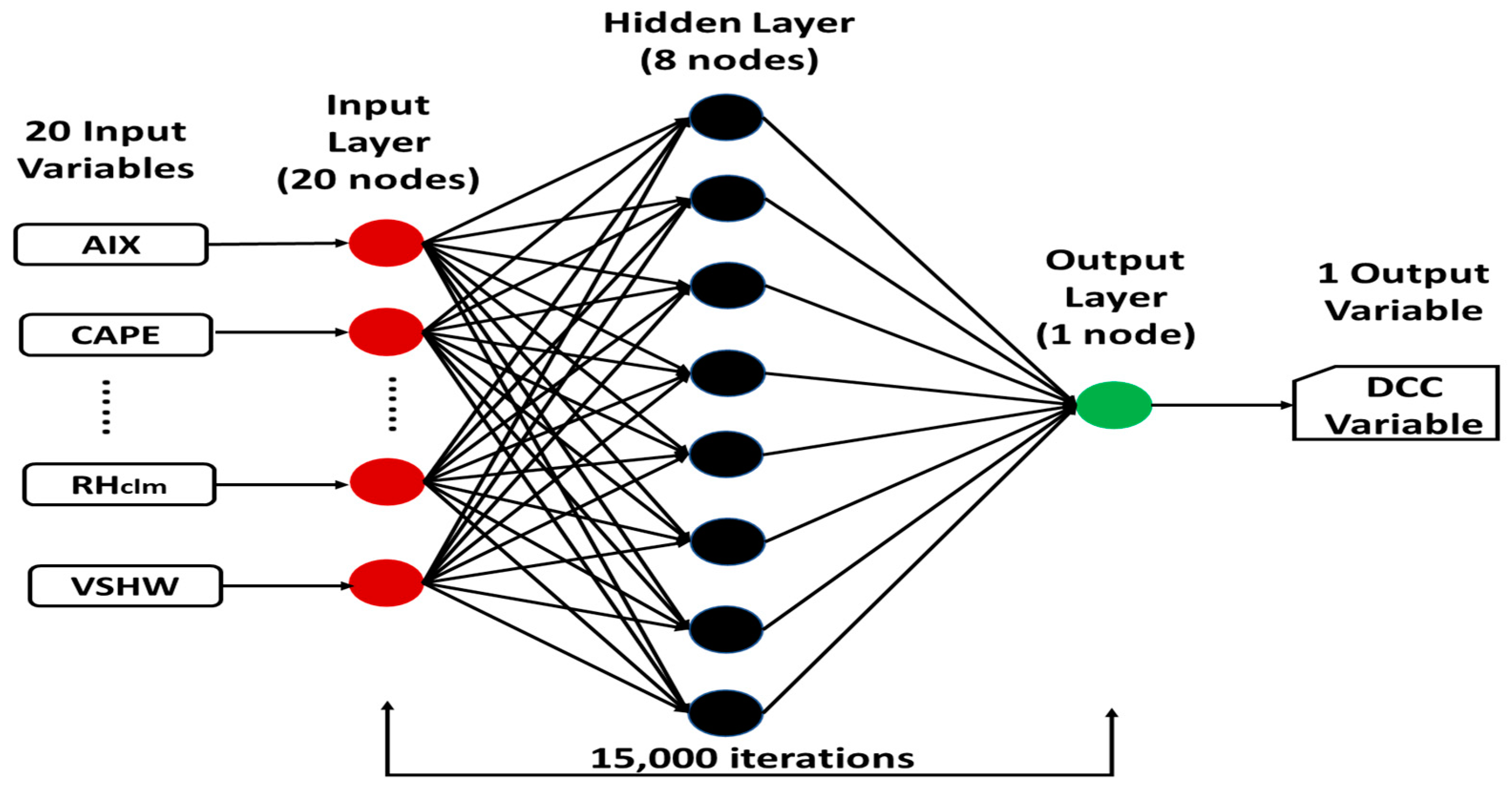
| BPNN | back-propagation neural network |
| CAPE | convective available potential energy |
| CCF | cloud cover fraction |
| CDR(s) | climate data record(s) |
| CFSR | climate forecast system reanalysis |
| COD | cloud optical depth |
| CPER | cloud particle effective radius |
| CTH | cloud top height |
| CTT | cloud top temperature |
| DCC(s) | deep convective cloud(s) |
| EOF | Empirical Orthogonal Function |
| EUMETSAT | European Organization for the Exploitation of Meteorological Satellites |
| GAC | global area coverage |
| HIRS | High-resolution Infra-Red Sounder |
| IWP | ice water path |
| NASA | National Aeronautics and Space Administration |
| MCS | mesoscale convective systems |
| MetOp | Meteorological Operational Satellites |
| MAI | covarying meteorology-aerosol invigoration |
| ML | machine learning |
| MODIS | Moderate-resolution Imaging Spectroradiometer |
| MSE | mean squared error |
| NAO | Northern Atlantic Ocean |
| NCEI | National Centers for Environmental Information |
| NCEP | National Centers for Environmental Prediction |
| NESDIS | National Environmental Satellite, Data, and Information Service |
| NH | northern hemisphere |
| NML | northern middle latitude |
| NOAA | National Oceanic and Atmospheric Administration |
| PAI | primary aerosol convective invigoration |
| PATMOS-x | Pathfinder Atmospheres-Extended |
| PC(s) | principal component(s) |
| POES | Polar Operational Environmental Satellites |
| PW | precipitable water |
| RH | relative humidity |
| SHAP | SHapley Additive exPlanation |
| SML | southern middle latitude |
| STAR | Center for Satellite Applications and Research |
| SVD | singular value decomposition |
| TRL | tropical latitude |
| UT | upper troposphere |
| VSHW | vertical shear of horizontal wind |
| WPO | Western Pacific Ocean |
| XGBoost | extreme gradient boosting (XGBoost) |
References
- Arakawa, A. The cumulus parameterization problem: Past, present, and future. J. Clim. 2004, 17, 2493–2525. [Google Scholar] [CrossRef]
- Futyan, J.M.; Del Genio, A.D. Deep convective system evolution over Africa and the tropical Atlantic. J. Clim. 2007, 20, 5041–5060. [Google Scholar] [CrossRef]
- Khain, A.; Rosenfeld, D.; Pokrovsky, A. Aerosol impact on the dynamics and microphysics of deep convective clouds. Q. J. Roy. Meteor. Soc. 2005, 131, 2639–2663. [Google Scholar] [CrossRef]
- Lohmann, U.; Feichter, J. Global indirect aerosol effects: A review. Atmos. Chem. Phys. 2005, 5, 715–737. [Google Scholar] [CrossRef]
- Stevens, B.; Feingold, G. Untangling aerosol effects on clouds and precipitation in a buffered system. Nature 2009, 461, 607–613. [Google Scholar] [CrossRef] [PubMed]
- Tao, W.K.; Chen, J.P.; Li, Z.Q.; Wang, C.; Zhang, C.D. Impact of Aerosols on Convective Clouds and Precipitation. Rev. Geophys. 2012, 50, 1–62. [Google Scholar] [CrossRef]
- Fan, J.W.; Wang, Y.; Rosenfeld, D.; Liu, X.H. Review of Aerosol-Cloud Interactions: Mechanisms, Significance, and Challenges. J. Atmos. Sci. 2016, 73, 4221–4252. [Google Scholar] [CrossRef]
- Seinfeld, J.H.; Bretherton, C.; Carslaw, K.S.; Coe, H.; DeMott, P.J.; Dunlea, E.J.; Feingold, G.; Ghan, S.; Guenther, A.B.; Kahn, R.; et al. Improving our fundamental understanding of the role of aerosol-cloud interactions in the climate system. Proc. Natl. Acad. Sci. USA 2016, 113, 5781–5790. [Google Scholar] [CrossRef] [PubMed]
- Li, Z.Q.; Rosenfeld, D.; Fan, J.W. Aerosols and their impact on radiation, clouds, precipitation, and severe weather events. Oxf. Res. Encycl. Environ. Sci. 2017, 1–36. [Google Scholar] [CrossRef]
- Fan, J.W.; Yuan, T.L.; Comstock, J.M.; Ghan, S.; Khain, A.; Leung, L.R.; Li, Z.Q.; Martins, V.J.; Ovchinnikov, M. Dominant role by vertical wind shear in regulating aerosol effects on deep convective clouds. J. Geophys. Res.-Atmos. 2009, 114, 1–9. [Google Scholar] [CrossRef]
- Grabowski, W.W. Untangling Microphysical Impacts on Deep Convection Applying a Novel Modeling Methodology. J. Atmos. Sci. 2015, 72, 2446–2464. [Google Scholar] [CrossRef]
- Grabowski, W.W.; Morrison, H. Untangling Microphysical Impacts on Deep Convection Applying a Novel Modeling Methodology. Part II: Double-Moment Microphysics. J. Atmos. Sci. 2016, 73, 3749–3770. [Google Scholar] [CrossRef]
- Zang, L.; Rosenfeld, D.; Pan, Z.X.; Mao, F.Y.; Zhu, Y.N.; Lu, X.; Gong, W. Observing Aerosol Primary Convective Invigoration and Its Meteorological Feedback. Geophys. Res. Lett. 2023, 50, 1–10. [Google Scholar] [CrossRef]
- Zhao, X.-P.; Dubovik, O.; Smirnov, A.; Holben, B.N.; Sapper, J.; Pietras, C.; Voss, K.J.; Frouin, R. Regional evaluation of an advanced very high resolution radiometer (AVHRR) two-channel aerosol retrieval algorithm. J. Geophys. Res. 2004, 109, D02204. [Google Scholar] [CrossRef]
- Zhao, T.X.P.; Chan, P.K.; Heidinger, A.K. A global survey of the effect of cloud contamination on the aerosol optical thickness and its long-term trend derived from operational AVHRR satellite observations. J. Geophys. Res.-Atmos. 2013, 118, 2849–2857. [Google Scholar] [CrossRef]
- Nakajima, T.; Higurashi, A.; Kawamoto, K.; Penner, J.E. A possible correlation between satellite-derived cloud and aerosol microphysical parameters. Geophys. Res. Lett. 2001, 28, 1171–1174. [Google Scholar] [CrossRef]
- Liu, J.J.; Li, Z.Q. Estimation of cloud condensation nuclei concentration from aerosol optical quantities: Influential factors and uncertainties. Atmos. Chem. Phys. 2014, 14, 471–483. [Google Scholar] [CrossRef]
- Stier, P. Limitations of passive remote sensing to constrain global cloud condensation nuclei. Atmos. Chem. Phys. 2016, 16, 6595–6607. [Google Scholar] [CrossRef]
- Heidinger, A.K.; Foster, M.J.; Walther, A.; Zhao, X.P. The Pathfinder Atmospheres-Extended Avhrr Climate Dataset. Bull. Am. Meteorol. Soc. 2014, 95, 909–922. [Google Scholar] [CrossRef]
- Foster, M.J.; Phillips, C.; Heidinger, A.K.; Borbas, E.E.; Li, Y.; Menzel, W.P.; Walther, A.; Weisz, E. PATMOS-x Version 6.0: 40 Years of Merged AVHRR and HIRS Global Cloud Data. J. Clim. 2023, 36, 1143–1160. [Google Scholar] [CrossRef]
- Heidinger, A.K.; Straka, W.C.; Molling, C.C.; Sullivan, J.T.; Wu, X.Q. Deriving an inter-sensor consistent calibration for the AVHRR solar reflectance data record. Int. J. Remote Sens. 2010, 31, 6493–6517. [Google Scholar] [CrossRef]
- Heidinger, A.K.; Evan, A.T.; Foster, M.J. A Naive Bayesian Cloud-detection Scheme Derived from CALIPSO and Applied withing PATMOS-x. J. Appl. Meteoro. Climat. 2012, 51, 1129–1144. [Google Scholar] [CrossRef]
- Walther, A.; Heidinger, A.K. Implementation of the Daytime Cloud Optical and Microphysical Properties Algorithm (DCOMP) in PATMOS-x. J. Appl. Meteorol. Clim. 2012, 51, 1371–1390. [Google Scholar] [CrossRef]
- Heidinger, A.K.; Cao, C.; Sullivan, J.T. Using Moderate Resolution Imaging Spectrometer (MODIS) to calibrate advanced very high resolution radiometer reflectance channels. J. Geophys. Res. 2002, 107, 4702. [Google Scholar] [CrossRef]
- Cao, C.; Weinreb, M.; Xu, H. Predicting Simultaneous Nadir Overpasses among Polar-Orbiting Meteorological Satellites for the Intersatellite Calibration of Radiometers. J. Atmos. Ocean. Technol. 2004, 21, 537–542. [Google Scholar] [CrossRef]
- Cao, C.Y.; Xiong, X.X.; Wu, A.H.; Wu, X.Q. Assessing the consistency of AVHRR and MODIS L1B reflectance for generating fundamental climate data records. J. Geophys. Res.-Atmos. 2008, 113, 1–10. [Google Scholar] [CrossRef]
- Pavolonis, M.J.; Heidinger, A.K.; Uttal, T. Daytime global cloud typing from AVHRR and VIIRS: Algorithm description, validation, and comparisons. J. Appl. Meteorol. 2005, 44, 804–826. [Google Scholar] [CrossRef]
- Zhao, X.; Foster, M.J. Analyzing Sensitive Aerosol Regimes and Active Geolocations of Aerosol Effects on Deep Convective Clouds over the Global Oceans by Using Long-Term Operational Satellite Observations. Climate 2022, 10, 167. [Google Scholar] [CrossRef]
- Saha, S.; Moorthi, S.; Pan, H.L.; Wu, X.R.; Wang, J.D.; Nadiga, S.; Tripp, P.; Kistler, R.; Woollen, J.; Behringer, D.; et al. The Ncep Climate Forecast System Reanalysis. Bull. Am. Meteorol. Soc. 2010, 91, 1015–1057. [Google Scholar] [CrossRef]
- Lundberg, S.M.; Erion, G.; Chen, H.; DeGrave, A.; Prutkin, J.M.; Nair, B.; Katz, R.; Himmelfarb, J.; Bansal, N.; Lee, S.I. From local explanations to global understanding with explainable AI for trees. Nat. Mach. Intell. 2020, 2, 56–67. [Google Scholar] [CrossRef]
- Hou, L.L.; Dai, Q.L.; Song, C.B.; Liu, B.W.; Guo, F.Z.; Dai, T.J.; Li, L.X.; Liu, B.S.; Bi, X.H.; Zhang, Y.F.; et al. Revealing Drivers of Haze Pollution by Explainable Machine Learning. Environ. Sci. Tech. Let. 2022, 9, 112–119. [Google Scholar] [CrossRef]
- Song, C.B.; Becagli, S.; Beddows, D.C.S.; Brean, J.; Browse, J.; Dai, Q.L.; Dall'Osto, M.; Ferracci, V.; Harrison, R.M.; Harris, N.; et al. Understanding Sources and Drivers of Size-Resolved Aerosol in the High Arctic Islands of Svalbard Using a Receptor Model Coupled with Machine Learning. Environ. Sci. Technol. 2022, 56, A–J. [Google Scholar] [CrossRef] [PubMed]
- Choudhary, I. A Step-By-Step Guide to Understand and Learn Shap (Shapley Additive Explaination) and How to Interpret ML Models Using the Shap Library. Available online: https://medium.com/@shahooda637/all-you-need-to-know-about-shap-for-explainable-ai-8ad35a05e6ec (accessed on 22 April 2023).
- Lundberg, S.M. SHAP Python Package. Available online: https://github.com/slundberg/shap (accessed on 1 May 2023).
- Molnar, C. Interpretable Machine Learning. Available online: https://christophm.github.io/interpretable-ml-book/shap.html (accessed on 14 April 2023).
- Atkinson, P.M.; Tatnall, A.R.L. Neural networks in remote sensing—Introduction. Int. J. Remote Sens. 1997, 18, 699–709. [Google Scholar] [CrossRef]
- Krizhevsky, A.; Sutskever, I.; Hinton, G.E. Imagenet classification with deep convolutional neural networks. Adv. Neural Inf. Process. Syst. 2012, 5, 1097–1105. [Google Scholar] [CrossRef]
- Zang, L.; Mao, F.Y.; Guo, J.P.; Wang, W.; Pan, Z.X.; Shen, H.F.; Zhu, B.; Wang, Z.M. Estimation of spatiotemporal PM, distributions in China by combining PM observations with satellite aerosol optical depth. Sci. Total Environ. 2019, 658, 1256–1264. [Google Scholar] [CrossRef]
- Bretherton, C.S.; Smith, C.; Wallace, J.M. An Intercomparison of Methods for Finding Coupled Patterns in Climate Data. J. Clim. 1992, 5, 541–560. [Google Scholar] [CrossRef]
- Wallace, J.M.; Smith, C.; Bretherton, C.S. Singular Value Decomposition of Wintertime Sea-Surface Temperature and 500-Mb Height Anomalies. J. Clim. 1992, 5, 561–576. [Google Scholar] [CrossRef]
- Newman, M.; Sardeshmukh, P.D. A Caveat Concerning Singular-Value Decomposition. J. Clim. 1995, 8, 352–360. [Google Scholar] [CrossRef]


| Variables | Note | |
|---|---|---|
| Aerosol | AIX | Satellite Observation |
| Cloud | CPER, COD, IWP, CCF, CTH, CTT | Satellite Observation |
| Meteorology | CAPE, PW, RHclm, RH850, RH400, RH2m, T850, T400, T2m, U850, U400, U10m, V850, V400, V10m, ω850, ω400, ωsig995, VSHW | CFSR Reanalysis |
| Cloud Variable (Aggregated SHAP Value) | 1st Important (SHAP Value) | 2nd Important (SHAP Value) | 3rd Important (SHAP Value) | Notes |
|---|---|---|---|---|
| CPER (3.26) | AIX (0.72) | VSHW (0.35) | RH850 (0.24) | AIE may manifest easily |
| COD (5.07) | T850 (1.04) | AIX (0.44) | RH400 (0.43) | AIE may not manifest easily |
| IWP (60.49) | RH400 (7.87) | VSHW (7.51) | AIX (6.20) | AIE may not manifest easily |
| CCF (0.02307) | V400 (0.00406) | RH400 (0.00403) | U400 (0.00395) | AIE may be concealed |
| CTH (0.63) | T400 (0.52) | U400 (0.11) | RH400 (0.10) | AIE may be concealed |
| CTT (2.93) | T400 (0.53) | CAPE (0.44) | RH2m (0.31) | AIE may be concealed |
| No | AIX/DCC PC1 Properties | Six DCC Variables | Comments | |||||
|---|---|---|---|---|---|---|---|---|
| CPER | COD | IWP | CCF | CTH | CTT | |||
| 1 | AIX PC1 Trend | (−) P (+) | (−) P (+) | (+) N (−) | (+) N (−) | (+) N (−) | (−) P (+) | (−) P (+): (from negative to positive) Positive trend (+) N (−): (from positive to negative) Negative trend |
| 2 | AIX PC1 Eigenvector | + | + | − | − | − | + | +: positive value −: negative value |
| 3 | AIX PC1 Variance | (−) P (+) | (−) P (+) | (−) P (+) | (−) P (+) | (−) P (+) | (−) P (+) | row1 × row2 |
| 4 | DCC PC1 Trend | (−) P (+) | (−) P (+) | (+) N (−) | (+) N (−) | (+) N (−) | (−) P (+) | (−) P (+): (from negative To positive) Positive trend (+) N (−): (from positive to negative) Negative trend |
| 5 | DCC PC1 Eigenvector | + | −/+ | − | − | − | −/+ | +: positive value −: negative value −/+: negative or positive |
| 6 | DCC PC1 Variance | (−) P (+) | (+) N (−)/(−) P (+) | (−) P (+) | (−) P (+) | (−) P (+) | (+) N (−)/(−) P (+) | row4 × row5 |
| 7 | Summary | P-AIE | N-/P-AIE | P-AIE | P-AIE | P-AIE | N-/P-AIE | N/P-AIE: negative/positive AIE |
| No | AIX/DCC PC1 Properties | 6 DCC Variables | Comments | |||||
|---|---|---|---|---|---|---|---|---|
| CPER | COD | IWP | CCF | CTH | CTT | |||
| 1 | AIX PC1 Trend | (+) N (−) | (−) P (+) | (+) N (−) | (−) P (+) | (+) N (−) | (+) N (−) | (−) P (+): (from negative to positive) Positive trend (+) N (−): (from positive to negative) Negative trend |
| 2 | AIX PC1 Eigenvector | − | + | − | + | − | − | +: positive value −: negative value |
| 3 | AIX Mode1 Variance | (−) P (+) | (−) P (+) | (−) P (+) | (−) P (+) | (−) P (+) | (−) P (+) | row1 × row2 |
| 4 | DCC PC1 Trend | (+) N (−) | (−) P (+) | (+) N (−) | (−) P (+) | (+) N (−) | (+) N (−) | (−) P (+): (from negative to positive) Positive trend (+) N (−): (from positive to negative) Negative trend |
| 5 | DCC PC1 Eigenvector | − | − | − | +/− | − | + | +: positive value −: negative value +/−: positive or negative |
| 6 | DCC Mode1 Variance | (−) P (+) | (+) N (−) | (−) P (+) | (−) P (+)/(+) N (−) | (−) P (+) | (+) N (−) | Row4 × row5 |
| 7 | Summary | P-AIE | N-AIE | P-AIE | P-/N-AIE | P-AIE | N-AIE | P/N-AIE: positive/negative AIE |
Disclaimer/Publisher’s Note: The statements, opinions and data contained in all publications are solely those of the individual author(s) and contributor(s) and not of MDPI and/or the editor(s). MDPI and/or the editor(s) disclaim responsibility for any injury to people or property resulting from any ideas, methods, instructions or products referred to in the content. |
© 2024 by the authors. Licensee MDPI, Basel, Switzerland. This article is an open access article distributed under the terms and conditions of the Creative Commons Attribution (CC BY) license (https://creativecommons.org/licenses/by/4.0/).
Share and Cite
Zhao, X.; Frech, J.; Foster, M.J.; Heidinger, A.K. Studying the Aerosol Effect on Deep Convective Clouds over the Global Oceans by Applying Machine Learning Techniques on Long-Term Satellite Observation. Remote Sens. 2024, 16, 2487. https://doi.org/10.3390/rs16132487
Zhao X, Frech J, Foster MJ, Heidinger AK. Studying the Aerosol Effect on Deep Convective Clouds over the Global Oceans by Applying Machine Learning Techniques on Long-Term Satellite Observation. Remote Sensing. 2024; 16(13):2487. https://doi.org/10.3390/rs16132487
Chicago/Turabian StyleZhao, Xuepeng, James Frech, Michael J. Foster, and Andrew K. Heidinger. 2024. "Studying the Aerosol Effect on Deep Convective Clouds over the Global Oceans by Applying Machine Learning Techniques on Long-Term Satellite Observation" Remote Sensing 16, no. 13: 2487. https://doi.org/10.3390/rs16132487
APA StyleZhao, X., Frech, J., Foster, M. J., & Heidinger, A. K. (2024). Studying the Aerosol Effect on Deep Convective Clouds over the Global Oceans by Applying Machine Learning Techniques on Long-Term Satellite Observation. Remote Sensing, 16(13), 2487. https://doi.org/10.3390/rs16132487