Abstract
Aerosol–cloud interactions play a crucial role in shaping Earth’s climate and hydrological cycle. Observing these interactions with high precision and accuracy is of the utmost importance for improving climate models and predicting Earth’s climate. Over the past few decades, lidar techniques have emerged as powerful tools for investigating aerosol–cloud interactions due to their ability to provide detailed vertical profiles of aerosol particles and clouds with high spatial and temporal resolutions. This review paper provides an overview of recent advancements in the study of ACI using lidar techniques. The paper begins with a description of the different cloud microphysical processes that are affected by the presence of aerosol, and with an outline of lidar remote sensing application in characterizing aerosol particles and clouds. The subsequent sections delve into the key findings and insights gained from lidar-based studies of aerosol–cloud interactions. This includes investigations into the role of aerosol particles in cloud formation, evolution, and microphysical properties. Finally, the review concludes with an outlook on future research. By reporting the latest findings and methodologies, this review aims to provide valuable insights for researchers engaged in climate science and atmospheric research.
1. Introduction
Aerosol and clouds are two fundamental components of the Earth’s atmosphere, exerting significant influences on climate, weather, and atmospheric chemistry. Aerosol is a suspension of tiny solid or liquid particles in air. Aerosol particles originate from natural sources such as dust storms, volcanic eruptions, and sea spray, as well as anthropogenic activities like industrial emissions and vehicle exhaust. Clouds, on the other hand, consist of water droplets or ice crystals suspended in the atmosphere, forming in response to changes in temperature, humidity, and atmospheric dynamics. It is well known that without aerosol particles, clouds would be a different phenomenon in their morphology and probably a rare occurrence in the atmosphere, since significant supersaturations of atmospheric water vapor are needed to trigger the homogeneous nucleation of the liquid phase [1,2,3,4]. Aerosol particles serve as nuclei for water vapor condensation at relatively low levels of supersaturation, thereby eliminating the need to achieve much higher supersaturation levels for condensation to take place. For this reason, the presence and characteristics of the aerosol particles are closely linked to the micro- and macrophysical properties of clouds. Conversely, clouds act as scavengers for atmospheric particles, both by exploiting them as condensation nuclei and by capturing aerosol through collision and coalescence processes. As a result, clouds serve as effective collectors for removing particles from the atmosphere, leading to their vertical redistribution, and finally, to deposition onto Earth’s surface through precipitation. Moreover, clouds can serve as reactive environments where aerosol particles undergo chemical transformations. Aqueous-phase reactions within cloud droplets can lead to the production or depletion of certain particle species through oxidation, acid–base reactions, and aqueous-phase chemistry, thus influencing atmospheric composition.
It is evident that studying the interaction between aerosol particles and clouds—two closely intertwined atmospheric components—represents a complex and dynamic phenomenon. This formidable challenge has significant implications for the climate system. Aerosol and clouds have direct radiative effects through scattering and absorbing solar and infrared radiation. But by far the most fascinating and complicated part of their interaction is that part by which different types and amounts of aerosol impact the properties of the clouds. Aerosol, due to its capability to serve as cloud condensation nuclei (CCN) or solid ice nucleating particles (INPs), affects cloud microphysical properties such as droplet size distribution, cloud albedo, and cloud lifetime. These properties of clouds in turn change their radiative behavior, which play a crucial role in regulating the planet’s temperature and climate variability. Furthermore, through these processes, such as cloud droplet nucleation and cloud phase transition, aerosol particles can influence precipitation processes, thus impacting regional rainfall patterns, droughts, extreme weather events, and the whole hydrological cycle. These aerosol effects, and their future projections, still have large margins of uncertainty.
A difficulty encountered in the study of aerosol-cloud-interaction (ACI) is that the effect of the aerosol on the morphological, microphysical, and radiative properties of clouds and on precipitation is mediated and conditioned by the dynamic and thermodynamic state of the atmosphere, so that it is a combination of many factors that finally determines the final state and fate of clouds. Given the complexity and interdependence of ACI, advanced observational techniques combined with modeling approaches are thus required to disentangle the mixing of factors, unravel underlying mechanisms, and quantify the impacts of aerosol on climate and the environment. In recent years, ACI has been the subject of many review articles [5,6,7,8,9,10,11] and its effects on the climate system have also been extensively surveyed [2,12,13,14,15,16]. We refer interested readers to these works for an in-depth overview of the current understanding of ACI.
Research into ACI employs a variety of approaches to understand the complex dynamics and implications for climate systems. The primary methodologies include in situ measurements, passive remote sensing, and active remote sensing. Each of these approaches provides unique insights and comes with specific advantages and limitations. In situ measurements involve direct sampling and analysis of aerosols and cloud particles using instruments onboard aircraft, ground stations, or ships. These measurements offer highly detailed and accurate data on aerosol properties (such as size distribution, chemical composition, and optical properties) and cloud microphysics (such as droplet size, liquid water content, and cloud condensation nuclei). These high-accuracy and -precision data deliver detailed information on aerosol physical and chemical properties and offer the advantage to conduct controlled experiments and calibrate remote sensing instruments. However, the spatial and temporal coverage is limited to the specific locations and times of measurement campaigns, and high operational costs and logistical challenges do not allow extensive space–time coverage, therefore they are limited to studying particular processes rather than continuous monitoring.
Passive remote sensing involves the detection of radiation, either emitted or reflected by aerosols and clouds. Instruments onboard satellites measure this radiation across various wavelengths to infer aerosol and cloud properties. Common passive sensors include radiometers and spectrometers. This approach allows global coverage and continuous monitoring, which allows long-term datasets, useful for studying trends and variability. Nevertheless, such indirect measurements can introduce uncertainties and require complex retrieval algorithms, have limited vertical resolution, and have potential difficulties in distinguishing between aerosol and optically thin cloud layers. Moreover, the dependence on sunlight restricts some measurements to daytime.
Some of these limitations are overcome by active remote sensing using instruments that emit electromagnetic radiation and measure the returned signal after interaction with aerosol and clouds. Lidar (light detection and ranging) and radar (radio detection and ranging) are the most common active sensors used in ACI studies. Such instruments provide vertical profiles of aerosol and cloud properties, can operate in both day and night conditions, and provide high spatial resolution and detailed characterization of aerosol and cloud layers. A drawback of these systems is that they are often complex and expensive, and often have limited spatial coverage compared to passive sensors.
Radars and lidars have distinct merits and drawbacks based on their operational principles and the specific information they provide. Radars operate in the microwave region of the electromagnetic spectrum, allowing them to penetrate through thick clouds and provide information on the internal structure of clouds and precipitation. So they are highly effective in detecting and quantifying precipitation, distinguishing between rain, snow, and hail and quantifying their intensity and distribution. Radars have a longer detection range than lidars, allowing for the observation of large atmospheric volumes and the tracking of weather systems over considerable distances. Moreover, unlike optical sensors, radars can operate in almost all weather conditions, including during heavy precipitation and cloudy skies. However, radars are far less sensitive than lidars to small aerosols and cloud droplets, making it challenging to accurately measure these smaller particles. In addition, the spatial resolution of radar systems is generally lower than that of lidar systems and this can limit the ability to resolve fine-scale features within clouds and aerosol layers. So radars are the primary choice for observing precipitation, internal cloud structures, and large-scale weather systems, due to their all-weather capability, long range, and detection efficacy for larger particles.
Lidars use laser light, typically in the ultraviolet, visible, or near-infrared regions, which is highly sensitive to small aerosol particles and cloud droplets. This allows for detailed characterization of aerosol properties and cloud microphysics, delivering high-resolution vertical profiles of aerosol and cloud layers, enabling detailed studies of their structure and dynamics. Probably the most important feature of lidars regarding ACI investigations is the ability to differentiate between various types of aerosol based on their optical properties, such as size, shape, and composition. Polarization lidar can further distinguish between spherical and non-spherical particles. Unfortunately, lidars struggle to penetrate through thick clouds and heavy precipitation, limiting their ability to observe the internal structure of deep cloud systems, and their range is generally shorter than that of radars, which can constrain the observation of large atmospheric volumes. Moreover, lidar performance is limited by atmospheric conditions such as fog, heavy aerosol loading, and daylight, particularly for systems operating in the visible spectrum. Their high sensitivity to small particles, high spatial and vertical resolution, and detailed aerosol characterization capability makes lidars particularly suitable for the study of aerosol while their limited penetration in thick clouds and shorter range, affected by certain atmospheric conditions, prevent their use in the study of large-scale weather systems.
Although radars and lidars provide complementary data, and their combined use can offer a more comprehensive understanding of ACI, in this review we focus on the contributions of lidar techniques to this field. Furthermore, to keep the article within reasonable dimensions, we seek to select results achieved by the lidar as a stand-alone instrument and only briefly mention its potential when used in synergy with other instruments. The article is organized as follows: In the next section, to provide the context, we will schematically illustrate the ways in which aerosol influences the main types of clouds. Subsequently, we describe the capabilities and recent developments of lidar technologies that allow to investigate aspects of ACI. Then, we report some main observational results presented in the recent literature and discuss some case studies. We then indicate the current challenges and limitations in studying ACI and propose future research directions and technological advancements, with emphasis on potential multi-instrument approaches to address remaining gaps.
2. Aerosol–Cloud Interactions
In a nutshell, aerosol can influence clouds in two directions: i. An aerosol increase, and consequently, a proportional increase in CCN, induces an increase in the number of cloud particles which, for the same amount of condensed water, leads to a corresponding decrease in their average dimension, and an increase in their surface area density (SAD), cloud optical thickness (), and albedo (). This is the well-known “Twomey effect” [17], observable in the different optical characteristics of continental (i.e., formed in an aerosol-rich atmosphere) compared to marine low-level clouds. An increase in cloud albedo for low-level clouds (“cloud brightening”) has a net cooling effect on climate [18]. This aerosol effect on mixed-phase and ice clouds is more complex due to the complicated mechanisms of ice nucleation, multiplication, and accretion and is dealt with later; ii. smaller cloud particles depress collision and coalescence, and consequently, delay or cancel the onset of precipitation, resulting in increased cloud extents, thicknesses, and lifetimes [19,20]. This “lifetime” or “Albrecht effect” further enhances planetary cooling. However, ACI are inserted into a complex of meteorological factors that call for feedback and adjustments, so the dominant effect of aerosol varies with respect to the type of cloud, its life phase, and its environment. The increase in lifetime is a well-documented effect for warm clouds, such as shallow cumulus and stratocumulus, while in mixed-phase clouds and in deep convection this aerosol effect is complicated by the dynamic processes and thermodynamics inside the cloud.
ACI parameters [21,22,23,24] are often used to quantify the aerosol effect: The indirect-effect parameter
with the aerosol particle extinction coefficient , usually measured at the cloud’s base, as a proxy for the aerosol load, describes the increase in the droplet number concentration with increasing aerosol load for constant liquid water path (LWP) (or liquid water content, LWC) conditions. Similar to , the nucleation efficiency parameter can be defined as
and quantifies the relative change in the cloud droplet effective radius with a relative change in the aerosol parameter. equals 3 for constant LWC according to the relationship. and can vary between zero (no dependence) and 0.33 and 1, respectively.
Below, we detail what is known about aerosol effects in relation to different types of clouds.
2.1. Liquid Clouds
Liquid clouds consist of tiny liquid water droplets that can exist at temperatures both above and slightly below freezing, whereas warm clouds specifically refer to those that form when the air temperature is above freezing. These are among the most interesting clouds from a climatic point of view given that, being low-altitude clouds, and therefore, dwelling at temperatures not significantly different from the surface, they reflect visible radiation without particularly influencing the infrared emission, so they are defined as one of the “air conditioners” of the climate system [25]. This effect is specifically important for marine stratocumulus that drastically change the surface albedo with respect to the ocean below [26]. Their study is simplified by the fact that their microphysics includes exclusively the gaseous and liquid phases. For such kinds of clouds it is well established that an increase in aerosol leads to an increase in the albedo, suppressing the collision–coalescence process, and therefore, depressing the rain, increasing the cloud lifetime and coverage.
At the cloud’s base, the number of CCN activated to become cloud droplets depends on the initial availability of CCN and on the updraft velocity. The activation of a particle of dry radius to a CCN depends on whether the supersaturation S exceeds its critical value , given by [27]
where A is the Kelvin coefficient, proportional to the surface tension and inversely proportional to temperature and is the hygroscopicity, a phenomenological parameter depending on the water activity of the solution [28]. The formula describes the fact that large, hygroscopic particles with low surface tension act more effectively as CCN. Aerosol particles take up water hygroscopically before they activate, thereby decreasing water vapor supersaturation, and this is even more the case when they activate and create droplets, so there is a ‘saturation’ mechanism with respect to their number density that makes the concentration of cloud droplets non-linearly dependent on the concentration of CCNs. Reutter et al. [29] identify two asymptotic regimes, one CCN-limited at small values of CCN concentration (few hundred ) and one updraft-limited (since the updraft speed in turn controls supersaturation) at high values of CCN concentration (several thousand ). In fact, in warm clouds, the droplet number concentration is influenced by both the availability of CCN and the strength of updrafts within the cloud. The transition from a CCN-limited regime to an updraft-limited regime can be explained as follows: i. in the CCN-limited regime the droplet number concentration in the cloud is primarily controlled by the availability of CCN. When there are few CCN present, not many droplets can form regardless of the updraft strength. Thus, in a CCN-limited regime, increasing the number of CCN leads to a corresponding increase in the droplet number; ii. however, as the number of CCN increases, more droplets form and there comes a point where the updraft velocity starts to play a more significant role. Updrafts cause adiabatic cooling and, together with the rate of droplet condensation, control supersaturation. When sufficient CCN are available, the ability of updrafts to continue lifting air parcels and supporting the formation of additional droplets becomes critical; iii. in the updraft-limited regime, the droplet concentration is primarily controlled by the strength of the updrafts since, even if the CCN concentration is high, the droplet concentration cannot increase significantly unless the updrafts are strong enough to support the continued formation and growth of cloud droplets and keep the supersaturation at high levels. Hence, when large concentrations of CCN are available, stronger updrafts are needed to provide enough cooling to maintain supersaturation and support further condensation.
Figure 1 shows these processes at work, where an increase in the concentration of CCN (on the horizontal axis) initially causes an increase in the concentration of cloud droplets (on the vertical axis) supported by high levels of supersaturation (color-coded in the figure). This CCN-limited regime ends up in a plateau where high CCN concentrations have no further effect on the concentration of cloud droplets, due to relatively low supersaturation, in this case not supported by sufficient vertical speed (updraft-limited regime). The data were collected in airborne measurement campaigns in 2013 [30].
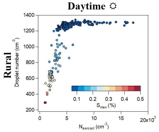
Figure 1.
Cloud droplet number vs. total aerosol number. Data are colored by maximum supersaturation. (Figure and caption from Figure 4 in Bougiatioti et al. [30], licensed under CC BY 4.0).
Since the concentration of cloud droplets is controlled by the CCN concentration, the latter can in turn control the cloud albedo . To evaluate this effect, for a cloud of geometric thickness h we write its optical thickness as
where is the cloud droplet size distribution, and —in the geometrical optics approximation—is the extinction efficiency. Introducing altitude-dependent effective radius and the liquid water content (LWC(z)) in a unit volume of air as
we can rearrange as
We can easily connect the cloud droplet concentration with the LWC through the droplet volume mean radius , and if the cloud droplet distribution is such that we write [31]
We can account for the non-adiabaticity of the cloud by defining the adiabatic fraction, , the ratio of the liquid water content (LWC) in a real cloud to the LWC that would be present if the cloud were strictly adiabatic, which represents the occurrence and amount of cloud mixing with the surrounding subsaturated air. is characterized by a large variability ( = 0.45 ± 0.21 according to Barlakas et al. [32]) driven by entrainment processes, but at the cloud base and close to its center we can assume that is close to 1 [33,34]. We can indicate with the rate of increase in LWC(z) with height in fully adiabatic conditions, a function of temperature and pressure ranging from 0.5 to 3 , that can be assumed to be relatively constant throughout the cloud depth for shallow clouds [35]. Thus, taking into account the entrainment of subsaturated air in the cloud, we can pose for LWC(z) at height z from the cloud base:
so we can write the cloud optical thickness in terms of and of the liquid water path (LWP), the amount of liquid water per unit area in the column of air from the cloud base to its top:
where . Finally, using Lacis and Hansen [36] and Meador and Weaver [37], we connect optical thickness and albedo :
where depends on the particle scattering phase function asymmetry, and can vary by a few units around 10.
So, Equations (10) and (11) tell us that increasing aerosol could produce higher cloud optical thickness and albedo (“cloud brightening”). Here, too, we note in both equations the presence of a ’saturation’ effect which makes the increase in optical thickness and albedo less and less relevant as the concentration of cloud droplets increases.
Opposed to those considerations, it should be noted that a greater number of cloud droplets with smaller size favors more evaporation. When droplets evaporate, the surrounding air cools and this can enhance the instability of the cloud and can increase the rate of entrainment, thus triggering the so-called “evaporation–entrainment feedback” [38]. This effect could sometimes overcome the cloud lifetime effect described above, in very polluted conditions [39]. In addition, a higher concentration of smaller droplets slows the sedimentation, which in turn may enhance the entrainment of dry air into the cloud, enhancing the droplet evaporation and reducing the albedo and water content, the so-called “sedimentation–entrainment feedback” [40].
For what concerns precipitation in warm clouds, the collision–coalescence rate that drives rain depends on [41], so should be greater than a threshold value ∼19 m, the so-called Hocking limit [42], to initiate rain within a cloud. Freud and Rosenfeld [43] demonstrated that the relationship between the number of activated cloud droplets near the cloud base and the cloud depth where reaches the threshold value is nearly linear. Since at the cloud base is positively influenced by the abundance of CCN, that means that deeper clouds need more CCN to suppress rain formation.
Complicating the picture is the fact that the presence of the aerosol itself has an effect on cloud deepening and on its overall macrostructure. In fact, there are some theoretical studies [44] and observations [45] that show how an increase in CCN can in fact invigorate the vertical development of clouds, increasing their thickness, LWP, and rain rate [46], as we will detail when treating in more detail the effect of aerosol on deep convective clouds. Moreover, in the case of marine stratocumulus, a change in the cloud decks from open cells to closed cells is documented as the aerosol increases compared to the background [47]. This has an effect on precipitation, since closed-cell clouds are reported be more stable and generally do not produce rain, whereas open cells, more prone to raining, dissipate as rain begins to fall.
To summarize, the warm cloud precipitation response to aerosol is predominantly to delay or suppress it. However, it is a complex and multifaceted process whose magnitude and direction depend on various factors, including aerosol properties, concentration, distribution, cloud regime and dynamics, and meteorological conditions. Figure 2 from Christensen et al. [48] reports a schematic of the micro- and macrophysical processes that regulates the warm stratocumulus morphology (upper panel). The interested reader can refer to the exhaustive review in Wood [26].
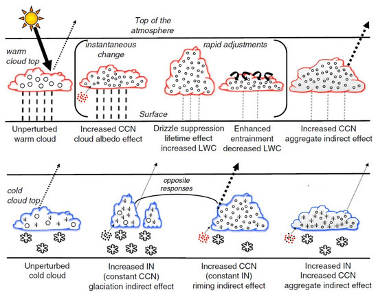
Figure 2.
Schematic diagram showing the various radiative mechanisms associated with aerosol indirect effects for warm (red outline) and mixed-phase (blue outline) clouds. Solid (dotted) arrows denote incident (reflected) shortwave radiation. An increase in CCN (batch of small red dots) instantaneously enhances cloud albedo by decreasing cloud droplet size (open circles). Rapid adjustments due to smaller droplets can affect precipitation (dashed lines) and entrainment (curved arrows). More IN (batch of small black dots) reduce cloud cover and albedo by causing greater amounts of cloud ice (small crystals) and solid precipitation (large crystals). More CCN in mixed-phase clouds decrease riming, thereby resulting in less precipitation. Increasing both CCN and IN results in relatively small changes in reflected sunlight and precipitation compared to the aggregate (combined) indirect effect in warm clouds. (Figure and caption from Figure 1 in Christensen et al. [48] ©Wiley. Used with permission).
2.2. Mixed-Phase Stratiform Clouds
These are low-altitude clouds composed of droplets of supercooled water and ice crystals, occurring at all latitudes and very frequent in the polar areas where they can have lifespans of many days. In mixed-phase clouds, the process of transferring water from the liquid to the solid phase (the Wegener–Bergeron–Findeisen (WBF) process) is likely to be more effective in a population of smaller cloud droplets, leading to larger ice crystals, and probably inducing greater precipitation and a shorter lifetime of the cloud (“glaciation effect”).
Among these types of clouds, the polar ones have attracted particular attention. Contrary to the behavior of their mid- and low-latitude counterparts, these clouds in polar regions do not have a large surface cooling effect because the sea ice at the surface is already bright so that the cloud-induced change in albedo is not significant. On the contrary, since the clouds also absorb IR radiation efficiently, they re-emit that energy back so that they could even warm the underlying surface. For these long lasting Arctic clouds, the ineffectiveness of the process of transferring water from the liquid to the solid phase (the Wegener–Bergeron–Findeisen (WBF) process) and the riming mechanism to complete the glaciation of these clouds is explained by the fact that the few ice particles nucleated at the top of the cloud, where the temperature is coldest due to radiative cooling, grow rapidly in its supersaturated environment and sediment out very fast, thus failing to complete the glaciation of the cloud [49]. The frequent presence of moist inversion layers above the cloud and the process of entrainment at the cloud top help to sustain the cloud. The cloud phase plays a key role in how it affects the polar surface radiation as glaciation can limit the cloud lifetime and render it less optically and thermally opaque, but still produce an overall positive radiative effect on the surface [50]. The lifetime of these clouds depends on the balance between CCN and INP concentrations. Studies have therefore focused on the effect not only of CCN but also of INPs, which are necessary to freeze liquid droplets at temperatures that are not low enough for homogeneous nucleation. The percentage of CCN that can act as INPs (about one particle in – acts as an INP) is thus a parameter of great importance, given that an increase in CCN at the expense of the INP component would lead to a greater number of small droplets, for which glaciation is less likely, and riming is less efficient, leading to a longer lifespan of the cloud, greater emissivity, and less precipitation. On the contrary, increasing the percentage of INPs leads to rapid glaciation, an enhancement of the WBP, and reduction in the duration of the cloud [51,52]. Aerosol types that can efficiently act as INPs are mineral dust, biological particles (pollen, bacteria, fungal spores and plankton), carbonaceous combustion products, soot, volcanic ash, and sea spray. Figure 2 from Christensen et al. [48] reports a schematic of the micro- and macrophysical processes that regulate the mixed-phase stratocumulus morphology (lower panel).
2.3. Deep Convective Clouds
Aerosol impacts deep convective clouds by changing how condensation and glaciation develop along the vertical, influencing not only the type and sizes of the condensate, but also the overall cloud’s dynamics through changes in latent heat release within the cloud. At the cloud’s base, an increase in CCN has the effect of creating more numerous and smaller droplets. In the warm part of the cloud, the additional SAD made available may be more efficient in reducing the supersaturation, so that more water can condense and the additional latent heat release can speed up the updraft. Moreover, smaller droplets may disfavor the onset of coalescence until high altitudes are reached. If the coalescence regime region lies above the freezing level, more liquid water can be transported aloft and made available to freezing. The enhanced latent heating release at those altitudes may further enhance the buoyancy and promote stronger updrafts. Both effects go in the direction of promoting convection strength. These are two declinations of a “convective invigoration” induced by the increase in aerosol [53,54]. Once ice starts forming, smaller cloud droplets and narrower size distributions enhance the WBF process but depress riming. However, the combined effect of increased CCN and INPs generally results in more efficient secondary ice multiplication due to the increased availability of supercooled droplets and initial ice crystals, which enhance interaction processes critical for secondary ice formation. Supercooled water droplets are essential for secondary ice formation processes like rime splintering (Hallett–Mossop process), when supercooled droplets collide with existing ice particles and freeze, causing splintering and the generation of additional ice crystals. Increasing CCN are responsible for greater numbers of supercooled droplets being available to collide with ice crystals, potentially enhancing the rime splintering process, while an increase in INPs leads to more primary ice crystals forming. This provides more initial ice particles that can interact with supercooled droplets or other ice crystals. Thus, higher concentrations of both CCN and INPs increase the number of interactions between supercooled droplets and ice crystals, enhancing processes like rime splintering. In addition to that, other secondary ice multiplication mechanisms such as mechanical fracturing of ice during collisions, sublimation, and condensation processes can also be influenced by increased CCN and INP concentrations. More initial ice crystals provide more opportunities for these processes to occur.
The depression of warm rain, and consequently, higher ice water content, may impact the formation of snow, graupel, and hail and enhance cloud electrification [55] and precipitation rates [56]. The formation of snow, graupel, and hail, along with the cold rain resulting from their melting, is influenced by the dynamic and thermodynamic structures of the clouds and the availability of giant cloud condensation nuclei CCN and INPs [57]. Smaller and narrower cloud droplet sizes and distribution, supercooled liquid water at greater altitude, enhanced cold rain and larger hail, higher cloud tops and stronger updrafts are effects clearly discernible at the scale of the single cloud. Figure 3 from Fan et al. [58] illustrates how an increase in aerosol in polluted environments is reflected in the increase in cloud-top height, cloudiness, and cloud thickness. Convective cores release a significant amount of smaller cloud ice particles, resulting in the extensive spread and prolonged dissipation of anvil clouds, as these smaller ice crystals fall more slowly.
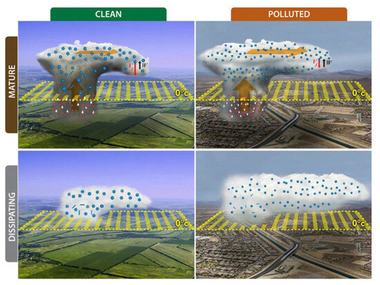
Figure 3.
Schematic illustration of the differences in cloud-top height (CTH), cloud fractions, and cloud thickness for storms in clean and polluted environments. Red dots denote cloud droplets, light blue dots represent raindrops, and blue shapes are ice particles. In the polluted environment, convective cores detrain larger amounts of cloud hydrometeors of much smaller size, leading to larger expansion and much slower dissipation of stratiform/anvil clouds resulting from smaller fall velocities of ice particles because of much reduced sizes. Therefore, larger cloud cover, higher CTHs, and thicker clouds are seen in the polluted storm after the mature stage. (Figure and caption from Figure 9 in Fan et al. [58]).
An increase in INPs can trigger a faster glaciation of the cloud, frequently resulting in the formation of precipitation via the ice–ice pathway (ice–ice collection and riming) at the expense of the mixed-phase pathway, thus depressing hail production.
Quantifying the impact of aerosols on a regional scale is more ambiguous, given that adjustments to the circulation and to the environment in which the cloud systems develop, are involved. An in-depth review of the interactions between aerosols and deep convective clouds can be found in [10].
2.4. Cirrus Clouds
These high-altitude ice clouds can be grouped into two types, according to their different origins and microphysical properties [59]: the first type forms directly as ice (in situ origin cirrus) within updrafts, nucleating both homogeneously and heterogeneously from the gas phase. The second type is composed of thick cirrus remnants of mixed-phase clouds, whose liquid droplets glaciated while lifted to a temperature below 235 K (liquid origin cirrus), where ice is formed heterogeneously, and possibly, homogeneously as well. In situ-origin cirrus are often thinner and have lower ice water content (IWC), while liquid-origin cirrus are mostly thick with a higher IWC and more numerous and larger ice crystals [60]. As ice formation can occur either from homogeneous nucleation of supercooled aqueous aerosol and cloud water droplets or heterogeneously from the small subset of solid aerosol that can act as INPs, the impact of aerosol on those clouds depends on which is the dominant mechanism. Which one between the two prevails depends on ambient temperature, relative humidity, and INP abundance. For those in situ-formed cirrus clouds whose origin can be dominated by homogeneous nucleation, an increase in INPs becomes significant if it can shift the prevailing nucleation mechanism towards the heterogeneous one. If so, the glaciation would involve a few INPs, resulting in larger sized but less numerous ice crystals [61,62]. For cirrus clouds of liquid origin, in cases where heterogeneous nucleation prevails, higher aerosol concentration corresponds to a larger density of smaller droplets, which leads to a greater number of ice particles with smaller dimensions, i.e., with lower sedimentation speeds, leading to a greater persistence of the cloud [63]. However, there are indications that the coupling between the amount of CCN and INPs with the concentration and morphology of ice crystals is weaker than with the concentration of cloud droplets for the case of warm clouds, and is more dependent on the meteorological and thermodynamic conditions governing the formation and lifetime of cirrus clouds [64].
Table 1 summarizes the responses of different cloud types to an increase in CCN or INPs.

Table 1.
Cloud response to an increase in CCN and IN.
3. Lidar Techniques for Studying Aerosol–Cloud Interactions
3.1. Lidar Fundamentals
Lidar technology has long been used to improve our understanding of atmospheric composition and dynamics, particularly for cloud and aerosol detection and atmospheric composition. The various configurations, including simple elastic lidar, polarization lidar, multiwavelength lidar, Raman lidar, high-spectral-resolution lidar (HSRL), differential absorption lidar (DIAL) and dual-field-of-view lidar, endow researchers with a comprehensive toolkit for probing atmospheric particulates. In its essence, the lidar emits pulses of laser light and detects, at a time t after the pulse was emitted, the light backscattered from the atmosphere at a distance . The factor 1/2 takes into account the double travel from the emitter to the illuminated volume at distance R and back to the colocated receiver. The backscattered light is collected with a telescope and detected with suitable sensors. The basic elastic Rayleigh lidar equation connecting the power received from the light backscattered from a distance R, P(R) at wavelength to the atmospheric optical parameters at R, formulated under the single-scattering hypothesis, is
where is the laser pulse power, and is the temporal length of the pulse, so that is the geometrical length of the volume illuminated by the laser light at a given time. The term O(R) is a function that represents the overlap of the laser beam and the receiver field of view, which is unity in the lidar far range (i.e., usually a few hundred of meters from it), and the solid angle is the angle at which the lidar views the light scattered from distance R. is the overall system efficiency. The term represents a constant contribution from the light conditions of the atmosphere and increases with the telescope field of view (FOV). The optical parameters of interest are the volume backscatter coefficient and the extinction coefficient , where the subscripts m and p refer to molecules and particles. While for their molecular part a link between the two quantities is provided by molecular scattering theory, resulting in , the ratio (also known as the lidar ratio, LR) is not known and depends on the particular aerosol. In general, we may pose, for a collection of scatterers with particle size distribution (PSD) (usually expressed in ),
In the case of spherical scatterers, the efficiencies can be computed in terms of Mie theory [65] and for non-absorbing aerosol their asymptotic values (i.e., for particle dimensions significantly greater than the lidar wavelenght) are, respectively, 1 and 2. There is no general analytical solution for scatterers of arbitrary shape and different approaches have been developed for those conditions [66]. Here, we want to underline how the lidar is essentially sensitive to the second moment of the PSD, i.e., to the averaged cross-sectional area of the particles.
The elastic Rayleigh lidar serves as the foundation of lidar-based aerosol detection, interpreting elastically backscattered light to estimate aerosol properties such as concentration and assess altitude distribution and optical thickness. As stated above, in Equation (12) two unknown quantities appear, so assumptions on the LR should be made in order to invert the equation [67,68] and different LRs should be carefully chosen with respect to different types of aerosols. This LR estimate can lead to large systematic errors in the retrieval of aerosol extinction coefficients [69,70] and should be performed carefully, taking into account the expected aerosol type, based on the geographical location and meteorological conditions of the measurement site [71]. The primary limitation of simple elastic Rayleigh lidar in studying ACI is its inability to differentiate between aerosol particles and cloud droplets due to their similar backscattering properties, leading to challenges in accurately characterizing their respective contributions and interactions.
Polarization diversity lidar enhances the aerosol classification capability by exploiting the polarization state of backscattered light, allowing for discrimination between different aerosol types based on their distinct polarization signatures. In fact, simple spherical particles backscatter the radiation with no change in its polarization state, while aspherical scatterers change the state of the incident polarization. This polarization diversity discrimination enables more accurate characterization of aerosol properties in terms of their morphology [72]. The parameter used in practice for lidar is the particle depolarization [73,74], defined as the ratio between the particle backscattering coefficients measured in two reception channels, one which selects the polarization parallel to that of the emitted light, the other the orthogonal one; with an obvious choice of symbols . depends on the size and shape of the particle: it is small for particles with dimensions smaller than the lidar wavelength and, as the particle dimension increases, it grows non-monotonically towards an asymptotic value that depends on the morphology of the particle [75]. Particle depolarization measurements are also useful for distinguishing the thermodynamical phase of cloud particles, as they can differentiate between spherical liquid droplets and non-spherical ice crystals based on the polarization characteristics of scattered light [72,76].
Despite its enhanced capability to differentiate between aerosols and cloud particles through polarization diversity, such setups still face limitations in accurately quantifying ACI due to their inability to provide detailed microphysical properties and precise particle size distributions.
Raman lidar can detect the vibrational Raman scattering from various atmospheric molecules, such as nitrogen, oxygen, ozone, water vapor, with each one resulting in distinctive shifts in the scattered wavelength. In the case of nitrogen molecules, Raman scattering detection offers the advantage of providing an additional, independent equation for the atmospheric extinction, allowing for a more accurate determination of the extinction coefficient, hence of the LR, without relying on assumptions about aerosol properties [77]. The spectrally resolved detection of the Raman rotational lines of and also allows the determination of the temperature of the atmosphere [78].
A different approach to disentangle the backscatter–extinction relationship is the one provided by the high-spectral-resolution lidar (HSRL), capable of resolving the spectrum of backscattered radiation at very high resolution, identifying and separating aerosol Mie scattering from molecular Cabannes–Brillouin scattering by the different amplitude of their Doppler line broadening, so the aerosol backscatter and extinction coefficient can be retrieved directly [79].
Raman and HSRL setups significantly enhance lidar’s potential by providing detailed measurements of aerosol optical properties with the ability to distinguish between different aerosols with high precision and accuracy [80,81].
Multiwavelength lidars further extend the capabilities of lidar systems by emitting laser pulses at multiple wavelengths, enabling the characterization of aerosols in terms of the spectral dependence of their scattering. This approach not only facilitates the differentiation between various aerosol types but provides valuable information about aerosol microphysics, optical properties, and aerosol size distribution [82,83]. For a typical two-wavelength lidar with , the ratio of the backscattering coefficients defines the color ratio (CR).
The differential absorption lidar (DIAL) technique utilizes two closely spaced laser wavelengths to probe the atmosphere, with one acting as a reference and the other being absorbed by a target gas, such as water vapor, enabling precise measurements of its concentration and vertical profiles [84].
Doppler lidars can measure the air-mass velocity in the atmosphere by analyzing the frequency shift (Doppler shift) of the backscattered light; Doppler lidar can determine the speed and direction of wind and other airborne particles. This technology is widely used in meteorology for wind profiling, turbulence detection, and studying atmospheric dynamics [85].
Fluorescence lidars utilize the property of certain aerosols and biological particles to emit fluorescence when excited by specific wavelengths of light. This technique allows for the detection and characterization of biological aerosols, organic compounds, and specific chemical species in the atmosphere. The enhanced capability of fluorescence lidars lies in their ability to identify and quantify specific aerosol types, such as biogenic or anthropogenic particles, providing valuable information on the sources and composition of aerosols within cloud systems [86,87].
Finally, different reception geometries of the backscattered signal, such as different telescopes at different receiving angles, or the use of different FOVs for the same receiving telescope, allow the estimation of some properties of the scattering medium, such as relevant portions of the phase function of the scatterers and other cloud properties as the extinction coefficient and particle effective radius [71,88].
The diverse capabilities of lidar technology, ranging from simple elastic lidar to more advanced configurations, allows us to effectively characterize aerosol in its dimensional component from about 0.1 m, thin clouds (i.e., with optical thicknesses less than 3), and in the case of thick clouds, the base of the cloud, and through the analysis of the signal along the depth of penetration into it, some microphysical characteristics of it.
The interested reader may refer to books on lidar’s application to atmospheric research, such as the classical Measures [89] or the more recent Weitkamp et al. [90].
3.2. Aerosol Characterization
3.2.1. Aerosol Classification
Basic lidar parameters for describing the particulate are the backscattering and extinction coefficients, extensive quantities dependent on the amount of particulate present in the investigation volume, its optical depth , and the particle linear depolarization ratio , with the lidar ratio LR and the color ratio CR as intensive quantities. These parameters are used to classify different aerosol types [91,92]. An example of aerosol classification is shown in Figure 4 from Groß et al. [93], where different types of aerosols are reported with respect to their , LR, and CR (in this case ratio of aerosol backscatter coefficient at 532 nm and 1064 nm). In their work, the authors report results from airborne measurement campaigns where a two-wavelength, polarization-diversity HSRL lidar was deployed from an aircraft, and the characterization results were validated by concomitant in situ measurements and Lagrangian analysis of the air masses being measured. From panel (a) in Figure 4 one can see that even a simpler single-wavelength polarization diversity lidar with the ability to measure LR either with HSRL or Raman approach is already effective in discerning different aerosol types. Basic elastic Rayleigh lidar with polarization diversity still allows aerosol classification if additional information is introduced in the classification algorithm, such as altitude, location, or surface type, suggesting the expected aerosol, as in the aerosol classification in the case of the satellite borne CALIOP lidar [94,95].
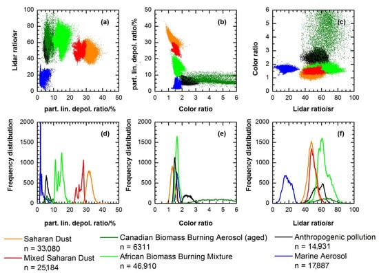
Figure 4.
Characteristic lidar quantities of various atmospheric aerosol types (a–c) with frequency distributions (d–f), as well as the total number of measurement points (n) for each aerosol type. Each point in (d–f) represents a single lidar observation. (Figure and caption from Figure 5 in Groß et al. [93] licensed under CC BY 3.0).
3.2.2. Aerosol Quantitative Specification
Of interest is estimates of quantities characterizing the aerosol distribution, such as particle mass density, SAD, volume density, particle mean, and effective radius. Such estimation has been carried out either by means of numerical simulations [96,97,98] or by comparing the lidar measurements with in situ measurements carried out in the same air mass probed by the lidar [99,100,101] to derive heuristic relationships.
A reconstruction of the aerosol PSD is possible starting from multiwavelength Raman/HRSL with polarization diversity lidars that can provide sets of extinction and backscattering coefficients [102]. In 2002, Veselovskii et al. [103] presented an inversion algorithm for the retrieval of particle size distribution parameters, i.e., mean or effective radius, number, surface area, and volume densities, and complex refractive index, from multiwavelength lidar data, and successively, Veselovskii et al. [104] used the extinction and backscattering coefficients at 355, 532, and 1064 nm to retrieve the parameters of a PSD expressed as a sum of two lognormals. Such kinds of retrievals, deriving the PSD in size ranges from fractions to a few tens of m, have been extensively used and have been validated with comparison to other independent remote sensing retrievals (i.e., inversions of spectral measurements of sky radiance and atmospheric transmittance from sun photometers) or colocated in situ data [105,106,107,108,109,110].
3.2.3. Aerosol Hygroscopicity
The aerosol’s hygroscopicity is an important factor determining its ability to act as a CCN. Lidars can detect changes in aerosol optical properties as they absorb water and grow. By monitoring these changes we can deduce hygroscopic scattering enhancement factors of different aerosol types. Ferrare et al. [111] used water vapor Raman lidar to simultaneously measure aerosol backscatter and RH and demonstrated how the increase in backscattering measured by the lidar can be correlated to RH, and Pahlow et al. [112] showed good correlations between a lidar-derived enhancement factor (measured over the range 85% RH to 96% RH) with the same parameter measured by a nephelometer (over the RH range 40% to 85%). More recently, Fernández et al. [113] investigated the hygroscopic characteristics using a multiwavelength water vapor Raman lidar and in situ aerosol observations. They inferred profiles of RH from water vapor Raman lidar data and described changes in aerosol optical properties under varying humidity conditions in terms of extinction enhancement, CR, and LR. Specifically, they found that increasing RH leads to aerosols absorbing water vapor, which increases their size, and consequently, decreases the CR while increasing the LR. They also estimated the RH-related scattering enhancement factor for the backscatter coefficient at 532 nm, which characterizes aerosols from a hygroscopic perspective. A similar study was conducted by Navas-Guzmán et al. [114] using continuous observations of aerosol backscatter coefficient, temperature, and water vapor mixing ratio from a water vapor Raman lidar system at the aerological station of MeteoSwiss in Payerne, Switzerland, since 2008.
Lv et al. [115] studied the extinction and backscattering coefficients at 355, 532, and 1064 nm to infer aerosol hygroscopicity according to an aerosol hygroscopic scattering enhancement factor , defined as the ratio between the particle backscatter coefficient when RH varies and that at a fixed RH, and using colocated lidar for backscatter coefficient profiles, and radiosondes for RH profiles. The homogeneity of the aerosol along the vertical was guaranteed by well-mixed conditions, assessed by concomitant measurement of potential temperature and water mixing ratio. Concurrent increases in the aerosol backscattering coefficient and RH were used to derive , then fitted to derive the parameters of the Kasten model [116]. Such derivations and comparison were performed for different types of aerosol and conditions. The lidar results were then compared to ground-based in situ data from a humidified nephelometer, showing good agreement. The relationship between the nephelometer-derived , which is based on the particle total scattering, and the one derived from a backscatter lidar was extensively addressed by Feingold and Morley [117], who compared lidar data with optical computations from airborne in situ measurements of aerosol size and composition. Lidar-derived enhancement factors may differ from the commonly used based on humidified nephelometers at RH greater than 95%. In such high-RH conditions, the lidar-derived enhancement factor is greater than the one from the computed extinctions that a nephelometer would measure. The disagreement is dependent on the PSD and aerosol composition. However, over the range 85% < RH < 95% the two factors were in reasonable agreement. Recently, other aerosol hygroscopic studies based on lidar measurements have been carried out, where backscatter and extinction enhancement factors are derived from lidar measurements and RH profiles are provided from radiosoundings or from water vapor lidar [118,119,120]. The amount of water vapor absorption by aerosols can also be inferred from the use of DIAL lidar, which simultaneously measures water vapor concentration and aerosol backscatter. In particular, this technique has proven effective in deriving the enhancement factor in a well mixed boundary layer capped by clouds [121]. We should stress the fact that lidars are useful tool for measuring aerosol growth not only because of their remote sensing capability, but also for conditions when RH > 85%, such as those encountered close to cloud bases, since for such elevated RH humidified nephelometers work poorly. It should be noted, however, that the hygroscopicity scattering enhancement factors measured with a nephelometer or a lidar and the growth factor measured with, for instance, a humidified tandem differential mobility analyzer (HTDMA) are both characterizing aerosol hygroscopic properties, but they are not identical. They represent different aspects of how aerosol particles interact with water vapor and how these interactions affect their optical properties (scattering) and physical properties (size) [122].
3.3. Cloud Characterization
3.3.1. Semi-Transparent Clouds
The semi-transparent clouds sampled by lidars predominantly belong to the cirrus cloud category, and it is on them that we focus. Cirrus clouds [123], characterized by their thin, wispy appearance and high altitudes, often exhibit optical transparency to varying degrees, allowing lidar systems to effectively penetrate entirely into these clouds, making them a primary focus of lidar-based research in atmospheric science. Given the extensive body of literature on cirrus lidar studies, we do not delve into exhaustive details on each aspect. Instead, we summarize lidar’s key capabilities in detecting and characterizing these clouds through various optical techniques. Readers interested in more comprehensive insights are encouraged to explore the rich literature of research in this field.
Basic backscatter lidars can identify cloud boundaries and reveal internal cloud structures [124,125,126]; scanning polarization diversity lidars provide insights into cloud particle phase [72], shape [127,128], orientation [129,130], and associated aerosols [131], with this capability being improved by the simultaneous use of more than one wavelength [132,133]; Raman or HSRL can provide calibrated data on ice water content, optical attenuation coefficient, and optical depth [134,135,136]. Ice water content can be also retrieved from optical extinction [137,138,139,140] and possibly validated by comparison with colocated in situ measurements [101,141]. Differential absorption lidar (DIAL) analyzes particle backscattering and determines water vapor density/relative humidity within the cirrus cloud environment [142]. Interestingly, information on the effective size of ice crystals in cirrus clouds can also be retrieved by measuring the fall speed that can be derived from lidar data [143,144].
3.3.2. Opaque Clouds
In lidar jargon, opaque clouds are those whose optical thickness exceeds 3. Lidars are not capable of probing them entirely; however, a penetration length within them can be defined in which the lidar is still able to produce a signal not totally attenuated for several tens of meters, and information can be obtained. Here, we focus predominantly on warm clouds, for which we can assume the cloud droplets to be spherical. This simplifies the treatment of multiple scattering within the cloud. The angular distribution of the light scattering from cloud droplets is a function of the effective size , and the forward scattering increases monotonically with the droplet dimension. Moreover, in such an optically dense medium, a significant amount of the backscattered light comes from multiple scattering.
Due to the lidar’s receiving geometry, most of the multi-scattered photons received come from small-angle forward scatterings plus a single backscattering at an angle close to 180°. Bissonnette et al. [145] describes an algorithm that uses multiple-field-of-view (FOV) lidar measurements between 1 and 12 mrad to retrieve the extinction coefficient at the lidar wavelength and the effective particle diameter, from which secondary products such as the LWC can be derived. These techniques have been used to characterize the structure of dense low-level water clouds [146].
Schmidt et al. [147] use two coaxial FOVs to detect the nitrogen Raman signal of light scattered in the forward direction by cloud droplets but backscattered inelastically by nitrogen. As the phase function for Raman scattering by nitrogen molecules is nearly isotropic in the backward direction, the scattering computation effort is significantly relieved as the angular distribution of the received light depends only on the scattering phase function of the droplets. In this way, the complication arising from the droplet size dependency of multiply-scattered light is eliminated, and this is an advantage with respect to the detection of multiple elastic scattering from droplets.
For cloud droplets, single-scattered light in the backward direction does not change its polarization state, while scattering events at different angles, which overall lead to backward scattering, change the polarization. So the profile of the polarization is related to the intensity of multiple scattering, in turn depending on particle size and concentration. Research has also explored the correlation between light depolarization induced by multiple scattering, measured across various fields of view (FOVs), and the characteristics of cloud droplet sizes [148,149]. Jimenez et al. [150] use lidar depolarization ratios at two different FOVs to retrieve microphysical properties of liquid-water clouds (cloud extinction coefficient, droplet effective radius, liquid water content, cloud droplet number concentration) in a cloud penetration depth of 100 m above the cloud base.
Donovan et al. [151] proposed a method that uses single-FOV observations of depolarization, under the assumption of a linear LWC increase with height (an assumption that corresponds to fixing the degree of non-adiabaticity of the cloud development) and constant cloud droplet number density at the cloud base. They used Monte Carlo multiple scattering modeling on a modified gamma function PSD to create a database for various values of LWC lapse rate, , different cloud-base heights, and different lidar FOVs. An optimal estimation Bayesian scheme was then used to infer profiles of and LWC as well as mean values of and the LWC lapse rate (from which the cloud subadiabaticity can be retrieved) within the cloud penetration length. Relatively few studies are available that exploit penetration depth in opaque cirrus clouds, due to the lack of knowledge of the phase function for ice crystal scattering [152].
It may seem limiting to only be able to sample the base of the cloud for only a few tens or hundreds of meters. However, the maximum supersaturation (above which no new CCN are activated) lies typically only a few tens of meters above the cloud base [153], so this is the region dictating the cloud droplet condensation, up to the level where collision/coalescence processes begin to take place. It is thus a region of utmost importance for cloud microphysical studies.
In cases where the LWP can be retrieved independently, from radars [154], microwave radiometers [155], or IR [156] and visible spectrometers [157], different approaches become viable. Grosvenor et al. [158] reviewed how passive satellite remote sensing retrieves cloud droplet number concentration () using cloud optical depth, cloud droplet effective radius (), and cloud-top temperature. Ground-based active remote sensing, on the other hand, relies on cloud radar reflectivity factor (Z) or the lidar extinction (backscatter) coefficient (, ), along with the microwave radiometer-retrieved liquid water path (LWP). To connect these retrievals, a droplet size distribution (DSD) assumption is necessary. For semi-transparent clouds, lidar-based retrievals offer an advantage because the optical parameters they measure depend on the second moment of the DSD, rather than the sixth moment as with radars. This sensitivity to makes lidar retrievals less dependent on the effective shape of the DSD. An empirical parameter k that equals the ratio of the mean volume radius to the mean effective radius [159] can be defined which implicitly incorporates the dependence on the DSD in the relation between , , and , which, from (14), (5), and (6), we can write as
at any given level in the cloud, thus linking to the lidar extinction [160]. Brenguier et al. [161] reported k parameter values ranging from 0.7 to 0.9 for stratiform clouds in various atmospheric conditions and cloud systems. In the absence of ancillary measurements for LWC, its profile can be guessed from the cloud-base temperature and pressure measurements by assuming an educated value for the adiabatic fraction , as in Equation (9).
4. Observational Results
4.1. Detection of CCN and INPs
Estimating concentrations of cloud condensation nuclei (CCN) is crucial for comprehending ACI. However, in situ observations of CCN are scarce, and many passive remote sensing methods can only offer proxies like total aerosol optical depth (AOD) for column-effective CCN assessments [162]. The potential of lidars in the study of ACI should be clear, and in this section we present some findings from observational studies using lidars to characterize the presence of CCN and INPs.
A method to extend the CCN spectrum measured at the surface to high altitudes was proposed by Ghan and Collins [163]. The lidar-measured value at altitude z where aerosol is exposed to the RH(z) is recalculated to the value it would have in dry conditions using an independent measurement of the vertical profile of RH and surface measurements made with a humidified nephelometer, providing the dependence of the extinction on relative humidity. A light-scattering hygroscopic growth factor is defined as the ratio between the extinction coefficient at various RHs and the extinction coefficient at dry conditions. The same factor is used also to quantify the amount of change in the particle backscattering coefficient due to water uptake: . Then, surface measurements of the CCN spectrum CCN() are scaled by the ratio of the backscatter (or extinction) profile to the backscatter (or extinction) retrieved at or near the surface, . This method assumes that the hygroscopic growth factor measured at the surface is the same as the one measured at z, and this implies the assumption that the vertical structure of CCN concentration is identical to the vertical structure of dry extinction or backscatter. These assumptions are equivalent to requiring that both the PSD shape (but not the total aerosol number) and the aerosol composition and particle shape are independent of altitude. In fact, Ghan et al. [164] showed that vertical inhomogeneity in the PSD, and presumably in particle shape and composition, are the main sources of error in such CCN retrievals, as near-surface CCN properties could be significantly different from CCN properties near the cloud base.
The ability of aerosols to act as CCN depends more on their size rather than chemical composition or mixing state [165]. This allows us to give an assessment on CCN through a determination of the aerosol PSD and an assessment of the number of particles whose dimension is above a certain threshold. It follows that in order to derive CCN concentration one should first use lidar-derived optical parameters to retrieve the aerosol PSD. Then, an assessment of particle hygroscopicity for different types of aerosol is needed to assess the ability of particles to act as CCN. In should be noted that high RH near clouds can change the aerosol optical properties and complicate the CCN retrieval.
Lv et al. [166] developed a method for profiling CCN concentrations that uses backscatter coefficients at 355, 532, and 1064 nm and extinction coefficients at 355 and 532 nm. Three types of aerosols (urban industrial, biomass burning, and dust) were considered, each with a different bimodal PSD. This PSD was inferred by using look-up tables developed based on the aerosol PSD database of the Aerosol Robotic Network (AERONET) database [167]. The best bimodal size distribution parameters were selected by comparing lidar observations and Mie optical computation [65] on the aerosol PSD, varying the PSD parameters through typical ranges for the three types of aerosols, until an agreement between measurement and calculations was reached. This “wet” PSD, measured at ambient RH, was then corrected to its “dry” version by using a hygroscopic scattering enhancement factor obtained from a humidified tandem differential mobility analyzer (HTDMA) or Water Vapour Raman lidar data. Then, the aerosol critical radius () for CCN activation at selected critical supersaturation was computed from the maximum of the -Köhler curve [28]. As, according to -Köhler theory, depends on the hygroscopicity parameter , which changes according to aerosol type, such that the critical radius () depends on the aerosol type, and for the three types of aerosols in the study it is taken from the literature [168,169,170]. CCN number concentrations are then determined from the integration of the retrieved PSD, from upward.
In 2019, Tan et al. [171] similarly proposed retrieving CCN concentrations from multiwavelength Raman lidar measurements, but instead of using the AERONET datasets and estimations of hygroscopicity according to aerosol classification, they relied on in situ-measured PSD, mixing states, and chemical composition data to define the relationship between CCN concentrations and lidar-derived optical properties. Hygroscopic enhancements of backscatter and extinction with relative humidity were used to create humidograms, to derive both dry backscatter and extinction and hygroscopicity at different wavelengths. These, together with lidar color ratios, extinctions, and backscatter data were used as input to a random forest regression machine learning algorithm that produced the best estimate for the ratio CCN-to-extinctions. Optical data simulated with Mie computations on in situ-measured PSD and the -Köhler curve from in situ-measured chemical composition were used as the training data. A similar in situ dataset was used as the test data.
Lenhardt et al. [172] explored the connections between aerosol backscatter and extinction coefficients using the airborne High-Spectral-Resolution Lidar 2 (HSRL-2) in biomass burning aerosol (BBA)-influenced air masses over the southeast Atlantic. They also examined in situ measurements of cloud condensation nuclei (CCN) concentrations that were spatiotemporally colocated. To ensure accuracy and avoid detecting swollen, highly hygroscopic aerosols that could artificially inflate backscatter and extinction values without corresponding increases in CCN concentration, observations taken at relative humidities (RHs) greater than 40% were filtered out. Their findings, illustrated in Figure 5, demonstrate robust linear relationships between lidar-derived backscatter and extinction coefficients and CCN concentration.
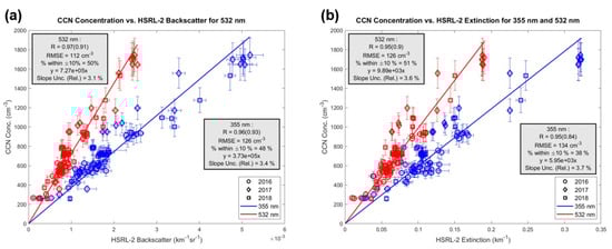
Figure 5.
CCN concentration versus HSRL−2 (a) backscatter and (b) extinction coefficients, with blue scatter points representing 355 nm and red scatter points representing 532 nm. This combined dataset represents 10 d of observations and 80 total colocated data points (per coefficient), covering all 3 years of ORACLES. Supersaturation for these observations ranges between 0.22% and 0.4%. The Pearson correlation coefficient is shown, with the Spearman rank correlation coefficient given in parentheses. Error bars are given for a CCN relative uncertainty of 10% and for calculated HSRL−2 uncertainties. Lines of best fit are forced through the origin to represent the practicality of using linear regression equations to quantitatively obtain CCN concentrations using HSRL−2 observables. (Figure and caption from Figure 3 in Lenhardt et al. [172] licensed under CC BY 4.0).
These studies employ multiwavelength Raman or HRSL lidars, commonly called 3 + 2 lidars, systems of a certain complexity, coupled with in situ measurements and RH profiling by means of radiosoundings or remote sensing. A simplified approach was suggested by Mamouri and Ansmann [173], who proposed an inversion algorithm for data from a more manageable single-wavelength polarization diversity lidar. This lidar is still able to specify aerosol classes (desert, non-desert continental, and marine). The possible presence of external mixing in the aerosol is handled by the procedure outlined in Tesche et al. [174]. Following a methodology proposed by Shinozuka et al. [175], extensive datasets from AERONET and lidar-correlated observations are then used to connect lidar-derived extinction to total particle number concentrations (for dry particle dimensions above defined thresholds depending on aerosol class) for the three aerosol classes. An evaluation of the correction for water uptake [28,176] is performed, this time assuming fixed RH values for the typical conditions of observation. Finally, a simple parametrization is used to connect the particle concentrations to the CCN concentrations, obtained from the former, with scaling factors dependent on supersaturation and aerosol class. Thus, height profiles of CCN concentrations can be retrieved from lidar-derived ambient aerosol extinction. This approach has lent itself to deriving global climatologies of CCN from the analysis of the satellite-borne lidar CALIOP [177]. A similar approach was also used by Choudhury and Tesche [178]. In their study, they employed normalized volume size distributions and refractive indices based on the CALIPSO aerosol model [94] for six aerosol types identified by the CALIPSO lidar. These size distributions were adjusted until agreement was reached between the extinction coefficient inferred from CALIPSO measurements and that calculated through light-scattering computations. These modified size distribution were then used to compute the aerosol number concentration for particles with dimension above defined thresholds depending on aerosol type. Again, the CCN concentration at a certain set of supersaturations was estimated by multiplying the aerosol number concentration by scaling factors, which depend on the aerosol type and on the level of supersaturation.
Lidars have been utilized to retrieve profiles of INP concentrations. This is achieved by integrating particle concentration profiles derived from lidar measurements with parameterizations of INP efficiency specific to different aerosol types and freezing mechanisms (such as immersion, condensation, deposition, or contact freezing). Mamouri and Ansmann [173] apply a regression of lidar-derived extinction vs. SAD to retrieve the INP concentration from the latter. Indeed, precise knowledge of aerosol type is crucial for using lidar retrievals to estimate INP concentrations. This is because INP concentrations are inferred solely from physical properties such as particle number concentration and/or size distribution (SAD), using parameterizations that have been developed for specific aerosol types. Examples include dust [179,180,181,182], marine aerosols [183], soot [181], and global aerosols [184]. Therefore, studies of INPs have typically focused on estimating INP concentrations within these specific aerosol classes.
Using a similar methodology, Haarig et al. [185] presented vertical profiles of cloud condensation nuclei (CCN) number concentration, particles with diameter greater than 500 nm, size distribution, mass, and INP concentration. These profiles were derived from measurements of 3 + 2 Raman lidar with polarization diversity. They compared these measurements with in situ CCN concentrations and INP-relevant aerosol properties collected by aircraft in the Saharan Air Layer (SAL) over the Barbados region.
Extinction coefficient profiles were separately retrieved for mineral dust, marine, and continental aerosols. Empirical conversion factors [186] were applied to convert these extinction coefficients into particle number concentrations (for particles above a threshold size dependent on aerosol type) and size distributions (SADs). Subsequently, various INP parameterizations [180,184] were tested, using particle number concentration and SAD as inputs.
Comparisons with in situ data of mass concentrations and particle number concentrations, which were used as inputs for the INP parameterizations, demonstrated good agreement.
Similarly, Marinou et al. [187] retrieved cloud-relevant particle number concentrations (i.e., particles whose linear dimensions in dry conditions are above 250 nm) and SADdry using lidar measurements from a + 2 Raman lidar with polarization diversity. INP concentration profiles were estimated using various ice nuclei parameterizations. These lidar-derived results were subsequently compared with direct INP measurements obtained by sampling aerosols along the lidar profile using two UAVs equipped with INP samplers. The collected samples were then analyzed offline using the FRIDGE (Frankfurt Ice Nucleation Deposition Freezing Experiment) INP counter [188]. This approach allowed them to evaluate the effectiveness of different INP parameterizations across different temperature ranges and types of particles.
Wieder et al. [189] also provided a direct validation of the INP concentration retrievals. They tested INP retrievals based on data from a + 2 Raman lidar with polarization diversity by comparing them with in situ observations of aerosols and INPs taken at a nearby mountain site in the Swiss Alps. The sampled air masses predominantly contained Saharan dust and continental aerosols. Various INP parameterizations were also evaluated in this study.
4.2. Impact of Aerosol on Mixed and Cirrus Clouds
Lidars are very effective in studying the impact of particular types of aerosols on the microphysics of clouds. Choi et al. [190] demonstrated the ability to distinguish supercooled liquid clouds from ice clouds for the satellite-borne lidar CALIOP from the layer-integrated particle depolarization ratio and backscatter coefficient at 532 nm, together with the cloud-top and -bottom temperatures, and demonstrated an inverse correlation between supercooled cloud presence and dust presence. Utilizing its capability to discriminate cloud phases, Tan et al. [191] directly investigated the ice-nucleating potential of dust, polluted dust, and smoke aerosols in mixed-phase clouds. They analyzed vertically resolved profiles of the cloud thermodynamic phase and aerosols from global spaceborne lidar data spanning 5 years. Their findings revealed that the presence of dust aerosols, both in their clean and polluted forms, in various regions globally, at temperatures conducive to mixed-phase clouds, reduces the fraction of supercooled clouds compared to total cloud cover in those regions. This reduction was attributed to the ability of dust aerosols to nucleate ice crystals.
The influence of desert dust aerosols on cirrus microphysical properties was investigated using concurrent and colocated datasets from CALIOP, CloudSat, and MODIS over the Taklimakan Desert [192]. The study highlighted the negative “Twomey effect” under arid conditions [62], where cloud albedo decreases due to increased heterogeneous nucleation. This process results in fewer but larger ice crystals, with higher fall velocities.
The role of wildfire smokes on cirrus formation was investigated by Mamouri et al. [193], who showed strong evidence that long-range transport of aged smoke (organic aerosol particles) originating from wildfires triggered significant ice nucleation, causing the formation of extended cirrus layers, upon gravity wave activity close to the tropopause.
The impact of aerosols on the cloud thermodynamic phase was also addressed by Zhang et al. [194] over east Asia by combining the 4-year datasets of CloudSat radar and CALIOP lidar measurements. Although temperature differences at the cloud top were shown to be the most important drivers of the cloud thermodynamic phase, regional differences and seasonal anomalies of glaciated and mixed-phase relative cloud fractions correlated well with variations in dust occurrence frequency. Moreover, the relative frequency of glaciated clouds associated with the concomitant presence of mineral dust was higher than the frequency of glaciated clouds associated with the presence of polluted dust, smoke, and background aerosols at any given cloud-top temperature.
Hofer et al. [195] investigated the efficiency of heterogeneous ice formation across stations located in New Zealand (Lauder), Germany (Leipzig), and southern Chile (Punta Arenas), as influenced by cloud-top temperature. They observed that Lauder and southern Chile, which typically experience low concentrations of free-tropospheric aerosols, exhibit lower ice formation efficiency compared to polluted mid-latitude regions like Germany. This suggests that the reduced ice formation efficiency at Lauder and Punta Arenas is linked to low concentrations of INPs. Additionally, episodes of continental aerosol outbreaks, more frequent at Lauder than Punta Arenas, moderately enhance the ice formation efficiency at Lauder relative to Punta Arenas.
The diurnal cycle of the supercooled water cloud fraction was investigated by Wang et al. [196] using 33 months of lidar observations from the Cloud–Aerosol Transport System aboard the International Space Station. This system provides cloud-top phase information at various local times within specific grid and isotherm parameters. The study revealed a strong and statistically significant negative correlation between the dust aerosol extinction coefficient near the location and time of liquid/ice cloud footprints, and the fraction of supercooled water clouds. Specifically, higher dust aerosol extinction coefficients corresponded to lower supercooled water cloud fractions in the observed regions.
4.3. Impact of Aerosol on Warm Clouds
Studies investigating the influence of aerosols on liquid clouds predominantly employ dual-FOV lidar techniques. These techniques allow for simultaneous measurement of cloud droplet size and number concentration. By capturing backscattered light at two different fields of view, this approach provides detailed vertical profiles of cloud microphysical properties, generally for several tens of meters up from the cloud base. The cloud base is a crucial region for the development of the cloud because it marks the altitude where rising air parcels reach their highest saturation levels and condensation begins. This initiation of condensation leads to the formation of cloud droplets, whose concentration remains essentially constant until the collision–coalescence process begins higher up in the cloud. So the processes occurring at the cloud base, including the activation of cloud condensation nuclei (CCN) and the subsequent formation of droplets, set the stage for the cloud’s microphysical properties. These initial conditions influence the cloud’s optical properties, precipitation potential, and overall dynamics.
Schmidt et al. [197] utilized colocated dual-FOV Raman lidar observations to examine aerosol and cloud optical and microphysical properties beneath and within thin-layered liquid-water clouds. They complemented these observations with Doppler lidar measurements of updrafts and downdrafts at the cloud base to explore the relationship between aerosol concentrations near the cloud base and cloud characteristics and dynamics.
The dual-FOV lidar setup enabled the use of two multiple-scattering channels (elastic and nitrogen Raman multiple-backscatter channels) to profile single-scattering extinction coefficient, effective radius, cloud droplet number concentration, and liquid water content [147]. The study included two case studies that tracked the evolution of altocumulus clouds in clean and moderately polluted conditions.
The impacts of updrafts, downdrafts, turbulent mixing, and entrainment of dry air on the microphysical properties of layered clouds were investigated using a combination of Doppler lidar and cloud radar. Significant differences in cloud properties were documented during updraft and downdraft episodes, particularly in droplet extinction, number concentration, and effective radius. Updraft episodes showed a notable increase in extinction coefficient and droplet number concentration, accompanied by lower droplet effective radii attributed to new droplet formation. The liquid water content (LWC) profile retrieved during updraft periods closely resembled the adiabatic LWC profile, whereas during downdraft episodes, higher LWC values indicated an absence of dry intrusions.
Conversely, signs of dry entrainment during downdrafts—such as lower effective radii and reduced LWC values observed around the cloud center—were documented in another case study. This scenario occurred when weaker vertical motions facilitated downward mixing of dry air from above the shallow cloud layer.
Various studies highlight the challenges of studying ACI in turbulent environments, where turbulent motions can influence processes like evaporation, drop collision, and new droplet formation, leading to opposing effects on cloud microphysical parameters [198]. Schmidt et al. [199] conducted a statistical analysis spanning two years, demonstrating a clear aerosol impact on cloud evolution and cloud droplet number concentration in the lower portions of altocumulus layers during updrafts. Their analysis underscored the importance of considering cloud dynamics in assessing ACI parameters, emphasizing the need to incorporate vertical wind information.
Furthermore, a comprehensive review of contemporary field studies on ACI in warm clouds (depicted in Figure 6) supported findings that Aitken- and accumulation-mode particles are activated at the cloud base when rapidly uplifted, irrespective of whether clouds form over oceans or continents. This dynamic contrasts with passive satellite remote sensing, which typically yields lower estimates of compared to ground-based lidar and airborne observations, potentially due to differences in cloud-top dynamics.
Figure 6.
values as published in the literature (see references to the right). Different methods (in situ measurements, remote sensing) and observational platforms (aircraft, satellite, ground based) are used. (Figure and caption from Figure 7 in Schmidt et al. [199] licensed under CC BY 4.0).
Jimenez et al. [200] conducted cloud measurements in pristine marine conditions at Punta Arenas in southern Chile using a multiwavelength polarization Raman lidar with a dual field of view (FOV), coupled with a Doppler lidar for vertical wind component measurements. They performed a detailed study on ACI, resolving updrafts and downdrafts. The study utilized profiles of aerosol-related parameters near the cloud base, cloud microphysical properties just above the cloud base, and 1-minute-resolution vertical wind data. CCN number concentration was derived from lidar-measured aerosol extinction following Mamouri and Ansmann [173]. They observed high values ranging from 0.8 to 1.0. The study highlighted the impact of aerosol water uptake on ACI, noting that the highest values were obtained when considering aerosol extinction measurements taken approximately 500 m below the cloud base (indicating dry aerosol conditions) in ACI computations.
Wang et al. [201] utilized a dual-FOV HSRL to simultaneously profile aerosols and liquid-water clouds, focusing on assessing the adiabaticity of these low-level clouds. They found in some cases that observed profiles of microphysical properties in these clouds are not perfectly adiabatic, contrary to common assumptions in current retrieval methods [202,203,204]. Additionally, the study confirmed that increased aerosol loading leads to higher droplet number concentrations and reduced droplet effective radius, although no discernible increase in liquid water path (LWP) was detected. This suggests that aerosol-induced water reduction through enhanced evaporation may offset increases caused by suppressed rain formation. The lidar observations were validated through concurrent measurements with cloud radar, Raman lidar, and sun photometer instruments.
5. Challenges and Future Directions
Up-to-date Earth System Model simulations that include a realistic description of microphysical properties and processes suggests that the equilibrium climate sensitivity (ECS) has been underestimated so far [205]. There are indications that the main reason for the increase in the current estimation of the ECS depends on the representation of processes involved in the formation of clouds and, specifically, on mixed-phase cloud microphysics and ACI [206,207].
Lidar techniques have significantly advanced our understanding of the complex interactions between aerosols, clouds, and the atmosphere; however, several challenges remain. Technological progress may partially increase the lidar capability demonstrated so far. The increasingly stringent demands of topographic mapping have led to lidar instruments whose vertical resolutions are well below one meter, and high-repetition laser systems allow temporal resolutions below one second. Enhancing the spatial and temporal resolution of lidar observations enables the detection of smaller-scale features within aerosol and cloud layers. High-resolution lidar systems allow for detailed mapping of aerosol and cloud properties with fine spatial granularity. Additionally, advancements in temporal resolution enable the study of rapid atmospheric processes, such as cloud evolution and aerosol transport, which can vary on short timescales. Lidars with a resolution at the submeter scale have been recently employed to sample the depth of the droplet activation layer of stratiform clouds with unprecedented accuracy [208].
Furthermore, we have limited our review mainly to works in which lidar could operate as an isolated instrument, but clearly the integration of multi-platform observations greatly increases its capacity. Combining data from various remote sensing instruments offers a more holistic view of ACI. By combining weather radars in the millimeter range and lidars, it is possible to detect a wider range of particle sizes and to more accurately determine cloud boundaries. Lidars, due to their shorter wavelength emissions, are capable of detecting particles from a few nanometers up to a few micrometers in size, but they may miss cloud droplets that are in the tens of micrometers range when their concentration is low. Conversely, radar backscatter is basically dependent on the sixth power of the droplet diameter, making it insensitive to small particles [209,210], hence the synergy between lidars and cloud radars enhances atmospheric observations by combining lidar’s high-resolution profiling of aerosols and cloud particles with cloud radar’s ability to detect larger hydrometeors and cloud structures, providing a comprehensive view of cloud microphysics and dynamics. IR [211], visible spectrometers [212], and microwave radiometers [213] further enhance such synergy, allowing a seamless retrieval between regions of the cloud detected by both radar and lidar and regions detected by just one of these two instruments, or having separate cloud and drizzle modes, or profiling the environmental temperature and LWC. Furthermore, the integration of remote sensors with in situ measurements within and around clouds, either airborne [214,215] or from high mountain research stations [189,216], greatly supports the study of ACI.
Satellite observations provide global coverage, aiding in the understanding of large-scale phenomena and their long-term evolution [217]. Leading the way was the CALIOP lidar, which operated in the A-Train and C-Train sun-synchronous orbits at an altitude of around 700 km for 17 years (2006–2023). The Cloud-Aerosol Transport System (CATS) followed, operated from the International Space Station for two and a half years (2015–2017), showcasing innovative technologies such as high-repetition frequencies. In 2022, China launched the Atmospheric Environment Monitoring Satellite (AEMS), equipped with its first space-borne atmospheric lidar, known as the Aerosol and Carbon Detection Lidar (ACDL), which operates in a 705 km solar-synchronous orbit, and includes two lidar instruments on a single platform. One of these instruments is the aerosol–cloud high-spectral-resolution lidar (ACHSRL) [218,219]. The now operational EarthCARE mission by ESA and JAXA includes the 355 nm HSR lidar ATLID, planned to operate for three or more years (2024–2027), and lastly, NASA’s AOS initiative, launched in 2022, aims to deploy at least one lidar on orbital platforms, scheduled for launch around 2030. Additionally, the Cloud and Aerosol Lidar for Global Scale Observations of the Ocean–Land–Atmosphere System (CALIGOLA), an advanced multi-purpose space lidar mission developed by the Italian Space Agency (ASI), is anticipated to launch around 2031 [108,220]. These ongoing and future space-based lidar missions will significantly enhance our understanding of ACI by providing high-resolution, three-dimensional measurements of aerosol distribution and cloud properties on a global scale.
At the same time, ground-based observation with large multiwavelength lidar systems with Raman or HSRL capabilities, innovative use of multiple FOV systems, possibly aided by radars and radiometers, will remain crucial for formulating and validating inversion techniques. These techniques, once validated, can then be applied to less advanced but more widely deployable systems and measurement stations. The detailed, continuous, and high-resolution vertical profiles provided by these systems are invaluable for distinguishing different types of aerosols, measuring the optical and microphysical properties of clouds and aerosols, and assessing their vertical distribution and temporal evolution.
Innovative unconventional algorithms are starting to be applied to large datasets. Machine learning (ML), for instance, can significantly enhance our capability to extract useful information from data. ML algorithms can automate the extraction of complex features such as cloud boundaries, aerosol layers, and cloud optical properties. Classification algorithms, such as support vector machines (SVMs) and convolutional neural networks (CNNs), can distinguish between different types of aerosols and cloud particles, improving the understanding of their interactions [221,222].
Supervised learning models can be trained on historical lidar data to predict the impact of aerosols on cloud properties like droplet size distribution and liquid water content [223], and regression models can estimate key parameters such as AOD and cloud droplet number concentration from lidar backscatter profiles. Unsupervised learning methods, such as clustering and anomaly detection algorithms, can identify unusual patterns or events in lidar data, such as unexpected changes in aerosol concentrations or cloud formation processes [224]. These anomalies can provide insights into rare or extreme ACI events, improving the understanding of their mechanisms.
Techniques like principal component analysis (PCA) [225,226] and t-distributed stochastic neighbor embedding (t-SNE) [224] can reduce the complexity of high-dimensional lidar data, making it easier to visualize and interpret aerosol and cloud interaction patterns. Improved visualization aids in hypothesis generation and data-driven discovery of ACI phenomena.
By applying these innovative methods of analysis to lidar data, researchers can enhance the precision, efficiency, and scope of ACI studies, leading to a deeper understanding of how aerosols affect cloud formation, development, and climate impacts.
6. Conclusions
This paper has presented a survey of diverse lidar techniques utilized to study ACI, emphasizing the capabilities and advancements in multiwavelength, Raman, and HSRL systems. Both ground-based and satellite lidar platforms have been discussed, highlighting their respective contributions to our understanding of aerosol properties and their role in cloud formation and dynamics. Multiwavelength lidar provides critical insights into the size distribution and optical properties of aerosols, allowing for detailed characterization of different aerosol types and their potential as cloud condensation nuclei (CCN). HSRL and Raman lidars enable precise separation of aerosol and molecular scattering components, delivering accurate AOD and backscatter profiles, as well as accurate aerosol classification. Raman water vapor lidar, by measuring water vapor and other gas profiles with high sensitivity, enhances our understanding of the humidity conditions under which aerosols interact with clouds, offering valuable data for modeling cloud microphysical processes. Dual-FOV depolarization lidars allow continuous measurements not limited to low-light background conditions and deliver precise characterization of aerosols and droplets within clouds, thus providing insights into the processes of aerosol-induced cloud nucleation.
The implementation of these lidar techniques has significantly advanced our knowledge of ACI, and, while ground-based lidar systems provide high-resolution, localized observations, which are critical for process-level studies, model validation and tests of new data interpretation schemes, satellite-based lidar extends the observation capability to a global scale, offering comprehensive coverage and the ability to monitor long-term trends and variability in ACI.
In conclusion, lidar technology has proven to be an indispensable tool in ACI studies. The advancements in multiwavelength, Raman, and HSRL techniques, combined with comprehensive ground-based and satellite observations, more accurate inversion, and innovative interpretation schemes for the data, provide a robust framework for addressing critical scientific questions about the role of aerosol in climate. Continued innovation and collaboration in this field will undoubtedly lead to deeper insights and advancements that enhance our ability to understand, model, and predict the complex interactions between aerosols, clouds, and climate.
Author Contributions
Writing—original draft, F.C.; Writing—review & editing, L.D.L., D.D. and M.S. All authors have undertaken bibliographic research and reviewing the state of the art. F.C. wrote the paper with contributions from all authors. All authors have read and agreed to the published version of the manuscript.
Funding
This research received no external funding.
Data Availability Statement
The original contributions presented in the study are included in the article, further inquiries can be directed to the corresponding author.
Conflicts of Interest
The authors declare no conflicts of interest.
Correction Statement
This article has been republished with a minor correction to Document Type. The type should change from "Article" to "Review". This change does not affect the scientific content of the article.
References
- Kaufman, Y.J.; Tanré, D.; Boucher, O. A satellite view of aerosols in the climate system. Nature 2002, 419, 215–223. [Google Scholar] [CrossRef] [PubMed]
- Seinfeld, J.H.; Bretherton, C.; Carslaw, K.S.; Coe, H.; DeMott, P.J.; Dunlea, E.J.; Feingold, G.; Ghan, S.; Guenther, A.B.; Kahn, R.; et al. Improving our fundamental understanding of the role of aerosol- cloud interactions in the climate system. Proc. Natl. Acad. Sci. USA 2016, 113, 5781–5790. [Google Scholar] [CrossRef] [PubMed]
- Li, J.; Carlson, B.E.; Yung, Y.L.; Lv, D.; Hansen, J.; Penner, J.E.; Liao, H.; Ramaswamy, V.; Kahn, R.A.; Zhang, P.; et al. Scattering and absorbing aerosols in the climate system. Nat. Rev. Earth Environ. 2022, 3, 363–379. [Google Scholar] [CrossRef]
- Carslaw, K.S. Chapter 2—Aerosol in the climate system. In Aerosols and Climate; Carslaw, K.S., Ed.; Elsevier: Amsterdam, The Netherlands, 2022; pp. 9–52. [Google Scholar] [CrossRef]
- Gordon, H.; Glassmeier, F.; T. McCoy, D. An Overview of Aerosol-Cloud Interactions. In Clouds and Their Climatic Impacts: Radiation, Circulation, and Precipitation; John Wiley & Sons, Inc.: Hoboken, NJ, USA, 2023; pp. 13–45. [Google Scholar]
- Michibata, T. Aerosol–cloud interactions in the climate system. In Handbook of Air Quality and Climate Change; Springer: Singapore, 2022; pp. 1–42. [Google Scholar]
- Kreidenweis, S.M.; Petters, M.; Lohmann, U. 100 years of progress in cloud physics, aerosols, and aerosol chemistry research. Meteorol. Monogr. 2019, 59, 11.1–11.72. [Google Scholar]
- Fan, J.; Wang, Y.; Rosenfeld, D.; Liu, X. Review of aerosol–cloud interactions: Mechanisms, significance, and challenges. J. Atmos. Sci. 2016, 73, 4221–4252. [Google Scholar] [CrossRef]
- Rosenfeld, D.; Andreae, M.O.; Asmi, A.; Chin, M.; de Leeuw, G.; Donovan, D.P.; Kahn, R.; Kinne, S.; Kivekäs, N.; Kulmala, M.; et al. Global observations of aerosol-cloud-precipitation-climate interactions. Rev. Geophys. 2014, 52, 750–808. [Google Scholar] [CrossRef]
- Tao, W.K.; Chen, J.P.; Li, Z.; Wang, C.; Zhang, C. Impact of aerosols on convective clouds and precipitation. Rev. Geophys. 2012, 50, RG2001. [Google Scholar] [CrossRef]
- Oreopoulos, L.; Cho, N.; Lee, D. A Global Survey of Apparent Aerosol-Cloud Interaction Signals. J. Geophys. Res. Atmos. 2020, 125, e2019JD031287. [Google Scholar] [CrossRef]
- Flossmann, A.I.; Wobrock, W. A review of our understanding of the aerosol–cloud interaction from the perspective of a bin resolved cloud scale modelling. Atmos. Res. 2010, 97, 478–497. [Google Scholar] [CrossRef]
- Bellouin, N.; Quaas, J.; Gryspeerdt, E.; Kinne, S.; Stier, P.; Watson-Parris, D.; Boucher, O.; Carslaw, K.S.; Christensen, M.; Daniau, A.L.; et al. Bounding global aerosol radiative forcing of climate change. Rev. Geophys. 2020, 58, e2019RG000660. [Google Scholar] [CrossRef]
- Tegen, I.; Schepanski, K. Climate feedback on aerosol emission and atmospheric concentrations. Curr. Clim. Chang. Rep. 2018, 4, 1–10. [Google Scholar] [CrossRef]
- Storelvmo, T. Aerosol effects on climate via mixed-phase and ice clouds. Annu. Rev. Earth Planet. Sci. 2017, 45, 199–222. [Google Scholar] [CrossRef]
- Carslaw, K.; Boucher, O.; Spracklen, D.; Mann, G.; Rae, J.; Woodward, S.; Kulmala, M. A review of natural aerosol interactions and feedbacks within the Earth system. Atmos. Chem. Phys. 2010, 10, 1701–1737. [Google Scholar] [CrossRef]
- Twomey, S. The supersaturation in natural clouds and the variation of cloud droplet concentration. Geofis. Pura Appl. 1959, 43, 243–249. [Google Scholar]
- Charlson, R.J.; Schwartz, S.; Hales, J.; Cess, R.D.; Coakley, J., Jr.; Hansen, J.; Hofmann, D. Climate forcing by anthropogenic aerosols. Science 1992, 255, 423–430. [Google Scholar] [CrossRef]
- Albrecht, B.A. Aerosols, cloud microphysics, and fractional cloudiness. Science 1989, 245, 1227–1230. [Google Scholar] [CrossRef] [PubMed]
- Rosenfeld, D.; Lensky, I.M. Satellite-based insights into precipitation formation processes in continental and maritime convective clouds. Bull. Am. Meteorol. Soc. 1998, 79, 2457–2476. [Google Scholar] [CrossRef]
- Feingold, G.; Remer, L.A.; Ramaprasad, J.; Kaufman, Y.J. Analysis of smoke impact on clouds in Brazilian biomass burning regions: An extension of Twomey’s approach. J. Geophys. Res. Atmos. 2001, 106, 22907–22922. [Google Scholar] [CrossRef]
- Garrett, T.; Zhao, C.; Dong, X.; Mace, G.; Hobbs, P. Effects of varying aerosol regimes on low-level Arctic stratus. Geophys. Res. Lett. 2004, 31, L17105. [Google Scholar] [CrossRef]
- McComiskey, A.; Feingold, G. Quantifying error in the radiative forcing of the first aerosol indirect effect. Geophys. Res. Lett. 2008, 35, L02810. [Google Scholar] [CrossRef]
- McComiskey, A.; Feingold, G.; Frisch, A.S.; Turner, D.D.; Miller, M.A.; Chiu, J.C.; Min, Q.; Ogren, J.A. An assessment of aerosol-cloud interactions in marine stratus clouds based on surface remote sensing. J. Geophys. Res. Atmos. 2009, 114, D09203. [Google Scholar] [CrossRef]
- Stephens, G.; Slingo, T. An air-conditioned greenhouse. Nature 1992, 358, 369–370. [Google Scholar] [CrossRef]
- Wood, R. Stratocumulus clouds. Mon. Weather Rev. 2012, 140, 2373–2423. [Google Scholar] [CrossRef]
- Ghan, S.J.; Abdul-Razzak, H.; Nenes, A.; Ming, Y.; Liu, X.; Ovchinnikov, M.; Shipway, B.; Meskhidze, N.; Xu, J.; Shi, X. Droplet nucleation: Physically-based parameterizations and comparative evaluation. J. Adv. Model. Earth Syst. 2011, 3, M10001. [Google Scholar] [CrossRef]
- Petters, M.D.; Kreidenweis, S.M. A single parameter representation of hygroscopic growth and cloud condensation nucleus activity. Atmos. Chem. Phys. 2007, 7, 1961–1971. [Google Scholar] [CrossRef]
- Reutter, P.; Su, H.; Trentmann, J.; Simmel, M.; Rose, D.; Gunthe, S.; Wernli, H.; Andreae, M.; Pöschl, U. Aerosol-and updraft-limited regimes of cloud droplet formation: Influence of particle number, size and hygroscopicity on the activation of cloud condensation nuclei (CCN). Atmos. Chem. Phys. 2009, 9, 7067–7080. [Google Scholar] [CrossRef]
- Bougiatioti, A.; Nenes, A.; Lin, J.J.; Brock, C.A.; de Gouw, J.A.; Liao, J.; Middlebrook, A.M.; Welti, A. Drivers of cloud droplet number variability in the summertime in the southeastern United States. Atmos. Chem. Phys. 2020, 20, 12163–12176. [Google Scholar] [CrossRef]
- Reid, J.S.; Hobbs, P.V.; Rangno, A.L.; Hegg, D.A. Relationships between cloud droplet effective radius, liquid water content, and droplet concentration for warm clouds in Brazil embedded in biomass smoke. J. Geophys. Res. 1999, 104, 6145–6153. [Google Scholar] [CrossRef]
- Barlakas, V.; Deneke, H.; Macke, A. The sub-adiabatic model as a concept for evaluating the representation and radiative effects of low-level clouds in a high-resolution atmospheric model. Atmos. Chem. Phys. 2020, 20, 303–322. [Google Scholar] [CrossRef]
- Lu, X.; Mao, F.; Rosenfeld, D.; Zhu, Y.; Zang, L.; Pan, Z.; Gong, W. The temperature control of cloud adiabatic fraction and coverage. Geophys. Res. Lett. 2023, 50, e2023GL105831. [Google Scholar] [CrossRef]
- Eytan, E.; Koren, I.; Altaratz, O.; Pinsky, M.; Khain, A. Revisiting adiabatic fraction estimations in cumulus clouds: High-resolution simulations with a passive tracer. Atmos. Chem. Phys. 2021, 21, 16203–16217. [Google Scholar] [CrossRef]
- Braun, R.A.; Dadashazar, H.; MacDonald, A.B.; Crosbie, E.; Jonsson, H.H.; Woods, R.K.; Flagan, R.C.; Seinfeld, J.H.; Sorooshian, A. Cloud adiabaticity and its relationship to marine stratocumulus characteristics over the northeast Pacific Ocean. J. Geophys. Res. Atmos. 2018, 123, 13–790. [Google Scholar] [CrossRef]
- Lacis, A.A.; Hansen, J. A parameterization for the absorption of solar radiation in the earth’s atmosphere. J. Atmos. Sci. 1974, 31, 118–133. [Google Scholar] [CrossRef]
- Meador, W.E.; Weaver, W.R. Two-Stream Approximations to Radiative Transfer in Planetary Atmospheres: A Unified Description of Existing Methods and a New Improvement. J. Atmos. Sci. 1980, 37, 630–643. [Google Scholar] [CrossRef]
- Xue, H.; Feingold, G. Large-Eddy Simulations of Trade Wind Cumuli: Investigation of Aerosol Indirect Effects. J. Atmos. Sci. 2006, 63, 1605–1622. [Google Scholar] [CrossRef]
- Chen, Y.C.; Christensen, M.; Xue, L.; Sorooshian, A.; Stephens, G.; Rasmussen, R.; Seinfeld, J. Occurrence of lower cloud albedo in ship tracks. Atmos. Chem. Phys. 2012, 12, 8223–8235. [Google Scholar] [CrossRef]
- Ackerman, A.S.; Kirkpatrick, M.P.; Stevens, D.E.; Toon, O.B. The impact of humidity above stratiform clouds on indirect aerosol climate forcing. Nature 2004, 432, 1014–1017. [Google Scholar] [CrossRef] [PubMed]
- Pruppacher, H.R.; Klett, J.D.; Wang, P.K. Microphysics of clouds and precipitation. Aerosol Sci. Technol. 1998, 28, 381–382. [Google Scholar] [CrossRef]
- Hocking, L.M. The collision efficiency of small drops. Q. J. R. Meteorol. Soc. 1959, 85, 44–50. [Google Scholar] [CrossRef]
- Freud, E.; Rosenfeld, D. Linear relation between convective cloud drop number concentration and depth for rain initiation. J. Geophys. Res. Atmos. 2012, 117, D02207. [Google Scholar] [CrossRef]
- Koren, I.; Dagan, G.; Altaratz, O. From aerosol-limited to invigoration of warm convective clouds. Science 2014, 344, 1143–1146. [Google Scholar] [CrossRef] [PubMed]
- Douglas, A.; L’Ecuyer, T. Global evidence of aerosol-induced invigoration in marine cumulus clouds. Atmos. Chem. Phys. 2021, 21, 15103–15114. [Google Scholar] [CrossRef]
- Altaratz, O.; Koren, I.; Remer, L.; Hirsch, E. Review: Cloud invigoration by aerosols—Coupling between microphysics and dynamics. Atmos. Res. 2014, 140–141, 38–60. [Google Scholar] [CrossRef]
- Rosenfeld, D.; Kaufman, Y.J.; Koren, I. Switching cloud cover and dynamical regimes from open to closed Benard cells in response to the suppression of precipitation by aerosols. Atmos. Chem. Phys. 2006, 6, 2503–2511. [Google Scholar] [CrossRef]
- Christensen, M.W.; Suzuki, K.; Zambri, B.; Stephens, G.L. Ship track observations of a reduced shortwave aerosol indirect effect in mixed-phase clouds. Geophys. Res. Lett. 2014, 41, 6970–6977. [Google Scholar] [CrossRef]
- Morrison, H.; De Boer, G.; Feingold, G.; Harrington, J.; Shupe, M.D.; Sulia, K. Resilience of persistent Arctic mixed-phase clouds. Nat. Geosci. 2012, 5, 11–17. [Google Scholar] [CrossRef]
- Coopman, Q.; Riedi, J.; Finch, D.; Garrett, T.J. Evidence for changes in arctic cloud phase due to long-range pollution transport. Geophys. Res. Lett. 2018, 45, 10–709. [Google Scholar] [CrossRef]
- Lance, S.; Shupe, M.; Feingold, G.; Brock, C.; Cozic, J.; Holloway, J.; Moore, R.; Nenes, A.; Schwarz, J.; Spackman, J.R.; et al. Cloud condensation nuclei as a modulator of ice processes in Arctic mixed-phase clouds. Atmos. Chem. Phys. 2011, 11, 8003–8015. [Google Scholar] [CrossRef]
- Ovchinnikov, M.; Korolev, A.; Fan, J. Effects of ice number concentration on dynamics of a shallow mixed-phase stratiform cloud. J. Geophys. Res. Atmos. 2011, 116, D00T06. [Google Scholar] [CrossRef]
- Sheffield, A.M.; Saleeby, S.M.; van den Heever, S.C. Aerosol-induced mechanisms for cumulus congestus growth. J. Geophys. Res. Atmos. 2015, 120, 8941–8952. [Google Scholar] [CrossRef]
- Rosenfeld, D.; Woodley, W.L.; Axisa, D.; Freud, E.; Hudson, J.G.; Givati, A. Aircraft measurements of the impacts of pollution aerosols on clouds and precipitation over the Sierra Nevada. J. Geophys. Res. Atmos. 2008, 113, D15203. [Google Scholar] [CrossRef]
- Williams, E.; Mushtak, V.; Rosenfeld, D.; Goodman, S.; Boccippio, D. Thermodynamic conditions favorable to superlative thunderstorm updraft, mixed phase microphysics and lightning flash rate. Atmos. Res. 2005, 76, 288–306. [Google Scholar] [CrossRef]
- Rosenfeld, D.; Bell, T.L. Why do tornados and hailstorms rest on weekends? J. Geophys. Res. Atmos. 2011, 116, D20211. [Google Scholar] [CrossRef]
- Cheng, C.T.; Wang, W.C.; Chen, J.P. Simulation of the effects of increasing cloud condensation nuclei on mixed-phase clouds and precipitation of a front system. Atmos. Res. 2010, 96, 461–476. [Google Scholar] [CrossRef]
- Fan, J.; Leung, L.R.; Rosenfeld, D.; Chen, Q.; Li, Z.; Zhang, J.; Yan, H. Microphysical effects determine macrophysical response for aerosol impacts on deep convective clouds. Proc. Natl. Acad. Sci. USA 2013, 110, E4581–E4590. [Google Scholar] [CrossRef]
- Krämer, M.; Rolf, C.; Luebke, A.; Afchine, A.; Spelten, N.; Costa, A.; Meyer, J.; Zöger, M.; Smith, J.; Herman, R.L.; et al. A microphysics guide to cirrus clouds–Part 1: Cirrus types. Atmos. Chem. Phys. 2016, 16, 3463–3483. [Google Scholar] [CrossRef]
- Luebke, A.E.; Afchine, A.; Costa, A.; Grooß, J.U.; Meyer, J.; Rolf, C.; Spelten, N.; Avallone, L.M.; Baumgardner, D.; Krämer, M. The origin of midlatitude ice clouds and the resulting influence on their microphysical properties. Atmos. Chem. Phys. 2016, 16, 5793–5809. [Google Scholar] [CrossRef]
- Kärcher, B.; Lohmann, U. A Parameterization of cirrus cloud formation: Homogeneous freezing including effects of aerosol size. J. Geophys. Res. Atmos. 2002, 107, 4698. [Google Scholar] [CrossRef]
- Kärcher, B.; Lohmann, U. A parameterization of cirrus cloud formation: Heterogeneous freezing. J. Geophys. Res. Atmos. 2003, 108, 4402. [Google Scholar] [CrossRef]
- Zhao, B.; Wang, Y.; Gu, Y.; Liou, K.N.; Jiang, J.H.; Fan, J.; Liu, X.; Huang, L.; Yung, Y.L. Ice nucleation by aerosols from anthropogenic pollution. Nat. Geosci. 2019, 12, 602–607. [Google Scholar] [CrossRef]
- Mülmenstädt, J.; Feingold, G. The radiative forcing of aerosol–cloud interactions in liquid clouds: Wrestling and embracing uncertainty. Curr. Clim. Chang. Rep. 2018, 4, 23–40. [Google Scholar] [CrossRef]
- Bohren, C.F.; Huffman, D.R. Absorption and Scattering of Light by Small Particles; John Wiley & Sons: Hoboken, NJ, USA, 2008. [Google Scholar]
- Mishchenko, M.I.; Hovenier, J.W.; Travis, L.D. Light scattering by nonspherical particles: Theory, measurements, and applications. Meas. Sci. Technol. 2000, 11, 1827. [Google Scholar]
- Klett, J.D. Stable analytical inversion solution for processing lidar returns. Appl. Opt. 1981, 20, 211–220. [Google Scholar] [CrossRef]
- Fernald, F.G. Analysis of atmospheric lidar observations: Some comments. Appl. Opt. 1984, 23, 652–653. [Google Scholar] [CrossRef]
- Sasano, Y.; Browell, E.V.; Ismail, S. Error caused by using a constant extinction/backscattering ratio in the lidar solution. Appl. Opt. 1985, 24, 3929–3932. [Google Scholar] [CrossRef]
- Kovalev, V.A. Sensitivity of the lidar solution to errors of the aerosol backscatter-to-extinction ratio: Influence of a monotonic change in the aerosol extinction coefficient. Appl. Opt. 1995, 34, 3457–3462. [Google Scholar] [CrossRef]
- Winker, D.M.; Vaughan, M.A.; Omar, A.; Hu, Y.; Powell, K.A.; Liu, Z.; Hunt, W.H.; Young, S.A. Overview of the CALIPSO Mission and CALIOP Data Processing Algorithms. J. Atmos. Ocean. Technol. 2009, 26, 2310–2323. [Google Scholar] [CrossRef]
- Sassen, K. The Polarization Lidar Technique for Cloud Research: A Review and Current Assessment. Bull. Am. Meteorol. Soc. 1991, 72, 1848–1866. [Google Scholar] [CrossRef]
- Cairo, F.; Donfrancesco, G.D.; Adriani, A.; Pulvirenti, L.; Fierli, F. Comparison of various linear depolarization parameters measured by lidar. Appl. Opt. 1999, 38, 4425–4432. [Google Scholar] [CrossRef]
- Gimmestad, G.G. Reexamination of depolarization in lidar measurements. Appl. Opt. 2008, 47, 3795–3802. [Google Scholar] [CrossRef]
- Liu, L.; Mishchenko, M.I. Constraints on PSC particle microphysics derived from lidar observations. J. Quant. Spectrosc. Radiat. Transf. 2001, 70, 817–831. [Google Scholar] [CrossRef][Green Version]
- Yoshida, R.; Okamoto, H.; Hagihara, Y.; Ishimoto, H. Global analysis of cloud phase and ice crystal orientation from Cloud-Aerosol Lidar and Infrared Pathfinder Satellite Observation (CALIPSO) data using attenuated backscattering and depolarization ratio. J. Geophys. Res. Atmos. 2010, 115, D00H32. [Google Scholar] [CrossRef]
- Ansmann, A.; Riebesell, M.; Weitkamp, C. Measurement of atmospheric aerosol extinction profiles with a Raman lidar. Opt. Lett. 1990, 15, 746–748. [Google Scholar] [CrossRef]
- Di Girolamo, P.; Marchese, R.; Whiteman, D.N.; Demoz, B.B. Rotational Raman Lidar measurements of atmospheric temperature in the UV. Geophys. Res. Lett. 2004, 31, L01106. [Google Scholar] [CrossRef]
- Eloranta, E.E. High spectral resolution lidar. In Lidar: Range-Resolved Optical Remote Sensing of the Atmosphere; Springer: New York, NY, USA, 2005; pp. 143–163. [Google Scholar]
- Burton, S.; Ferrare, R.; Vaughan, M.; Omar, A.; Rogers, R.; Hostetler, C.; Hair, J. Aerosol classification from airborne HSRL and comparisons with the CALIPSO vertical feature mask. Atmos. Meas. Tech. 2013, 6, 1397–1412. [Google Scholar] [CrossRef]
- Müller, D.; Ansmann, A.; Mattis, I.; Tesche, M.; Wandinger, U.; Althausen, D.; Pisani, G. Aerosol-type-dependent lidar ratios observed with Raman lidar. J. Geophys. Res. Atmos. 2007, 112, D16202. [Google Scholar] [CrossRef]
- Müller, H.; Quenzel, H. Information content of multispectral lidar measurements with respect to the aerosol size distribution. Appl. Opt. 1985, 24, 648–654. [Google Scholar] [CrossRef]
- Böckmann, C.; Mironova, I.; Müller, D.; Schneidenbach, L.; Nessler, R. Microphysical aerosol parameters from multiwavelength lidar. J. Opt. Soc. Am. A 2005, 22, 518–528. [Google Scholar] [CrossRef]
- Browell, E.V.; Carter, A.; Shipley, S.T.; Allen, R.; Butler, C.; Mayo, M.; Siviter, J.; Hall, W. NASA multipurpose airborne DIAL system and measurements of ozone and aerosol profiles. Appl. Opt. 1983, 22, 522–534. [Google Scholar] [CrossRef]
- Hill, C. Coherent focused lidars for Doppler sensing of aerosols and wind. Remote. Sens. 2018, 10, 466. [Google Scholar] [CrossRef]
- Immler, F.; Engelbart, D.; Schrems, O. Fluorescence from atmospheric aerosol detected by a lidar indicates biogenic particles in the lowermost stratosphere. Atmos. Chem. Phys. 2005, 5, 345–355. [Google Scholar] [CrossRef]
- Veselovskii, I.; Hu, Q.; Goloub, P.; Podvin, T.; Korenskiy, M.; Pujol, O.; Dubovik, O.; Lopatin, A. Combined use of Mie–Raman and fluorescence lidar observations for improving aerosol characterization: Feasibility experiment. Atmos. Meas. Tech. 2020, 13, 6691–6701. [Google Scholar] [CrossRef]
- Hutt, D.L.; Bissonnette, L.R.; Durand, L. Multiple field of view lidar returns from atmospheric aerosols. Appl. Opt. 1994, 33, 2338–2348. [Google Scholar] [CrossRef] [PubMed]
- Measures, R. Laser Remote Sensing: Fundamentals and Applications; Krieger Publishing Company: Malabar, FL, USA, 1992. [Google Scholar]
- Weitkamp, C. Range-Resolved Optical Remote Sensing of the Atmosphere; Springer: New York, NY, USA, 2005; Volume 102, pp. 241–303. [Google Scholar]
- Papagiannopoulos, N.; Mona, L.; Amodeo, A.; D’Amico, G.; Gumà Claramunt, P.; Pappalardo, G.; Alados-Arboledas, L.; Guerrero-Rascado, J.L.; Amiridis, V.; Kokkalis, P.; et al. An automatic observation-based aerosol typing method for EARLINET. Atmos. Chem. Phys. 2018, 18, 15879–15901. [Google Scholar] [CrossRef]
- Floutsi, A.A.; Baars, H.; Engelmann, R.; Althausen, D.; Ansmann, A.; Bohlmann, S.; Heese, B.; Hofer, J.; Kanitz, T.; Haarig, M.; et al. DeLiAn—A growing collection of depolarization ratio, lidar ratio and Ångström exponent for different aerosol types and mixtures from ground-based lidar observations. Atmos. Meas. Tech. 2023, 16, 2353–2379. [Google Scholar] [CrossRef]
- Groß, S.; Esselborn, M.; Weinzierl, B.; Wirth, M.; Fix, A.; Petzold, A. Aerosol classification by airborne high spectral resolution lidar observations. Atmos. Chem. Phys. Discuss. 2012, 12, 2487–2505. [Google Scholar] [CrossRef]
- Omar, A.H.; Winker, D.M.; Vaughan, M.A.; Hu, Y.; Trepte, C.R.; Ferrare, R.A.; Lee, K.P.; Hostetler, C.A.; Kittaka, C.; Rogers, R.R.; et al. The CALIPSO Automated Aerosol Classification and Lidar Ratio Selection Algorithm. J. Atmos. Ocean. Technol. 2009, 26, 1994–2014. [Google Scholar] [CrossRef]
- Kim, M.H.; Omar, A.H.; Tackett, J.L.; Vaughan, M.A.; Winker, D.M.; Trepte, C.R.; Hu, Y.; Liu, Z.; Poole, L.R.; Pitts, M.C.; et al. The CALIPSO Version 4 Automated Aerosol Classification and Lidar Ratio Selection Algorithm. Atmos. Meas. Tech. 2018, 11, 6107–6135. [Google Scholar] [CrossRef]
- Gobbi, G.P. Lidar estimation of stratospheric aerosol properties: Surface, volume, and extinction to backscatter ratio. J. Geophys. Res. Atmos. 1995, 100, 11219–11235. [Google Scholar] [CrossRef]
- Barnaba, F.; Gobbi, G.P. Lidar estimation of tropospheric aerosol extinction, surface area and volume: Maritime and desert-dust cases. J. Geophys. Res. Atmos. 2001, 106, 3005–3018. [Google Scholar] [CrossRef]
- Dionisi, D.; Barnaba, F.; Diémoz, H.; Di Liberto, L.; Gobbi, G.P. A multiwavelength numerical model in support of quantitative retrievals of aerosol properties from automated lidar ceilometers and test applications for AOT and PM10 estimation. Atmos. Meas. Tech. 2018, 11, 6013–6042. [Google Scholar] [CrossRef]
- Jäger, H.; Hofmann, D. Midlatitude lidar backscatter to mass, area, and extinction conversion model based on in situ aerosol measurements from 1980 to 1987. Appl. Opt. 1991, 30, 127–138. [Google Scholar] [CrossRef]
- Mona, L.; Marenco, F. Lidar Observations of Volcanic Particles. In Volcanic Ash; Elsevier: Amsterdam, The Netherlands, 2016; pp. 161–173. [Google Scholar]
- Snels, M.; Cairo, F.; Di Liberto, L.; Scoccione, A.; Bracaglia, M.; Deshler, T. Comparison of Coincident Optical Particle Counter and Lidar Measurements of Polar Stratospheric Clouds Above McMurdo (77.85°S, 166.67°E) from 1994 to 1999. J. Geophys. Res. Atmos. 2021, 126, e2020JD033572. [Google Scholar] [CrossRef]
- Müller, D.; Wandinger, U.; Ansmann, A. Microphysical particle parameters from extinction and backscatter lidar data by inversion with regularization: Simulation. Appl. Opt. 1999, 38, 2358–2368. [Google Scholar] [CrossRef] [PubMed]
- Veselovskii, I.; Kolgotin, A.; Griaznov, V.; Müller, D.; Wandinger, U.; Whiteman, D.N. Inversion with regularization for the retrieval of tropospheric aerosol parameters from multiwavelength lidar sounding. Appl. Opt. 2002, 41, 3685–3699. [Google Scholar] [CrossRef] [PubMed]
- Veselovskii, I.; Kolgotin, A.; Griaznov, V.; Müller, D.; Franke, K.; Whiteman, D.N. Inversion of multiwavelength Raman lidar data for retrieval of bimodal aerosol size distribution. Appl. Opt. 2004, 43, 1180–1195. [Google Scholar] [CrossRef]
- Müller, D.; Mattis, I.; Ansmann, A.; Wehner, B.; Althausen, D.; Wandinger, U.; Dubovik, O. Closure study on optical and microphysical properties of a mixed urban and Arctic haze air mass observed with Raman lidar and Sun photometer. J. Geophys. Res. Atmos. 2004, 109, D13206. [Google Scholar] [CrossRef]
- Veselovskii, I.; Dubovik, O.; Kolgotin, A.; Lapyonok, T.; Di Girolamo, P.; Summa, D.; Whiteman, D.N.; Mishchenko, M.; Tanré, D. Application of randomly oriented spheroids for retrieval of dust particle parameters from multiwavelength lidar measurements. J. Geophys. Res. Atmos. 2010, 115, D21203. [Google Scholar] [CrossRef]
- Alados-Arboledas, L.; Müller, D.; Guerrero-Rascado, J.L.; Navas-Guzmán, F.; Pérez-Ramírez, D.; Olmo, F.J. Optical and microphysical properties of fresh biomass burning aerosol retrieved by Raman lidar, and star-and sun-photometry. Geophys. Res. Lett. 2011, 38, L01807. [Google Scholar] [CrossRef]
- Di Girolamo, P.; De Rosa, B.; Summa, D.; Franco, N.; Veselovskii, I. Measurements of Aerosol Size and Microphysical Properties: A Comparison Between Raman Lidar and Airborne Sensors. J. Geophys. Res. Atmos. 2022, 127, e2021JD036086. [Google Scholar] [CrossRef]
- Sannino, A.; Amoruso, S.; Damiano, R.; Scollo, S.; Sellitto, P.; Boselli, A. Optical and microphysical characterization of atmospheric aerosol in the Central Mediterranean during simultaneous volcanic ash and desert dust transport events. Atmos. Res. 2022, 271, 106099. [Google Scholar] [CrossRef]
- Sorrentino, A.; Sannino, A.; Spinelli, N.; Piana, M.; Boselli, A.; Tontodonato, V.; Castellano, P.; Wang, X. A Bayesian parametric approach to the retrieval of the atmospheric number size distribution from lidar data. Atmos. Meas. Tech. 2022, 15, 149–164. [Google Scholar] [CrossRef]
- Ferrare, R.A.; Melfi, S.H.; Whiteman, D.N.; Evans, K.D.; Poellot, M.; Kaufman, Y.J. Raman lidar measurements of aerosol extinction and backscattering: 2. Derivation of aerosol real refractive index, single-scattering albedo, and humidification factor using Raman lidar and aircraft size distribution measurements. J. Geophys. Res. Atmos. 1998, 103, 19673–19689. [Google Scholar] [CrossRef]
- Pahlow, M.; Feingold, G.; Jefferson, A.; Andrews, E.; Ogren, J.A.; Wang, J.; Lee, Y.N.; Ferrare, R.A.; Turner, D.D. Comparison between lidar and nephelometer measurements of aerosol hygroscopicity at the Southern Great Plains Atmospheric Radiation Measurement site. J. Geophys. Res. Atmos. 2006, 111, D05S15. [Google Scholar] [CrossRef]
- Fernández, A.; Apituley, A.; Veselovskii, I.; Suvorina, A.; Henzing, J.; Pujadas, M.; Artíñano, B. Study of aerosol hygroscopic events over the Cabauw experimental site for atmospheric research (CESAR) using the multi-wavelength Raman lidar Caeli. Atmos. Environ. 2015, 120, 484–498. [Google Scholar] [CrossRef]
- Navas-Guzmán, F.; Martucci, G.; Collaud Coen, M.; Granados-Muñoz, M.J.; Hervo, M.; Sicard, M.; Haefele, A. Characterization of aerosol hygroscopicity using Raman lidar measurements at the EARLINET station of Payerne. Atmos. Chem. Phys. 2019, 19, 11651–11668. [Google Scholar] [CrossRef]
- Lv, M.; Liu, D.; Li, Z.; Mao, J.; Sun, Y.; Wang, Z.; Wang, Y.; Xie, C. Hygroscopic growth of atmospheric aerosol particles based on lidar, radiosonde, and in situ measurements: Case studies from the Xinzhou field campaign. J. Quant. Spectrosc. Radiat. Transf. 2017, 188, 60–70. [Google Scholar] [CrossRef]
- Kasten, F. Visibility forecast in the phase of pre-condensation. Tellus 1969, 21, 631–635. [Google Scholar] [CrossRef]
- Feingold, G.; Morley, B. Aerosol hygroscopic properties as measured by lidar and comparison with in situ measurements. J. Geophys. Res. Atmos. 2003, 108, 4327. [Google Scholar] [CrossRef]
- Bedoya-Velásquez, A.E.; Navas-Guzmán, F.; Granados-Muñoz, M.J.; Titos, G.; Román, R.; Casquero-Vera, J.A.; Ortiz-Amezcua, P.; Benavent-Oltra, J.A.; de Arruda Moreira, G.; Montilla-Rosero, E.; et al. Hygroscopic growth study in the framework of EARLINET during the SLOPE I campaign: Synergy of remote sensing and in situ instrumentation. Atmos. Chem. Phys. 2018, 18, 7001–7017. [Google Scholar] [CrossRef]
- Dawson, K.W.; Ferrare, R.A.; Moore, R.H.; Clayton, M.B.; Thorsen, T.J.; Eloranta, E.W. Ambient Aerosol Hygroscopic Growth From Combined Raman Lidar and HSRL. J. Geophys. Res. Atmos. 2020, 125, e2019JD031708. [Google Scholar] [CrossRef]
- Zhao, Y.; Wang, X.; Cai, Y.; Pan, J.; Yue, W.; Xu, H.; Wang, J. Measurements of atmospheric aerosol hygroscopic growth based on multi-channel Raman-Mie lidar. Atmos. Environ. 2021, 246, 118076. [Google Scholar] [CrossRef]
- Wulfmeyer, V.; Feingold, G. On the relationship between relative humidity and particle backscattering coefficient in the marine boundary layer determined with differential absorption lidar. J. Geophys. Res. Atmos. 2000, 105, 4729–4741. [Google Scholar] [CrossRef]
- Jefferson, A.; Hageman, D.; Morrow, H.; Mei, F.; Watson, T. Seven years of aerosol scattering hygroscopic growth measurements from SGP: Factors influencing water uptake. J. Geophys. Res. Atmos. 2017, 122, 9451–9466. [Google Scholar] [CrossRef]
- Lynch, D.; Sassen, K.; Starr, D.; Stephens, G.; Bailey, M.; Hallett, J.; Heymsfield, A.; Mcfarquhar, G.; DeMott, P.; Wylie, D.; et al. Cirrus; Oxford University Press: Oxford, UK, 2002. [Google Scholar] [CrossRef]
- Giannakaki, E.; Balis, D.S.; Amiridis, V.; Kazadzis, S. Optical and geometrical characteristics of cirrus clouds over a Southern European lidar station. Atmos. Chem. Phys. 2007, 7, 5519–5530. [Google Scholar] [CrossRef]
- Gouveia, D.A.; Barja, B.; Barbosa, H.M.J.; Seifert, P.; Baars, H.; Pauliquevis, T.; Artaxo, P. Optical and geometrical properties of cirrus clouds in Amazonia derived from 1 year of ground-based lidar measurements. Atmos. Chem. Phys. 2017, 17, 3619–3636. [Google Scholar] [CrossRef]
- Cairo, F.; De Muro, M.; Snels, M.; Di Liberto, L.; Bucci, S.; Legras, B.; Kottayil, A.; Scoccione, A.; Ghisu, S. Lidar observations of cirrus clouds in Palau. Atmos. Chem. Phys. 2021, 21, 7947–7961. [Google Scholar] [CrossRef]
- Noel, V.; Chepfer, H.; Ledanois, G.; Delaval, A.; Flamant, P.H. Classification of particle effective shape ratios in cirrus clouds based on the lidar depolarization ratio. Appl. Opt. 2002, 41, 4245–4257. [Google Scholar] [CrossRef] [PubMed]
- Cairo, F.; Deshler, T.; Di Liberto, L.; Scoccione, A.; Snels, M. A study of optical scattering modelling for mixed-phase polar stratospheric clouds. Atmos. Meas. Tech. 2023, 16, 419–431. [Google Scholar] [CrossRef]
- Kaul, B.V.; Samokhvalov, I.V.; Volkov, S.N. Investigating particle orientation in cirrus clouds by measuring backscattering phase matrices with lidar. Appl. Opt. 2004, 43, 6620–6628. [Google Scholar] [CrossRef]
- Noel, V.; Chepfer, H. A global view of horizontally oriented crystals in ice clouds from Cloud-Aerosol Lidar and Infrared Pathfinder Satellite Observation (CALIPSO). J. Geophys. Res. Atmos. 2010, 115, D00H23. [Google Scholar] [CrossRef]
- Qi, S.; Huang, Z.; Ma, X.; Huang, J.; Zhou, T.; Zhang, S.; Dong, Q.; Bi, J.; Shi, J. Classification of atmospheric aerosols and clouds by use of dual-polarization lidar measurements. Opt. Express 2021, 29, 23461–23476. [Google Scholar] [CrossRef] [PubMed]
- Beyerle, G.; Schäfer, H.J.; Neuber, R.; Schrems, O.; McDermid, I.S. Dual wavelength lidar observation of tropical high-altitude cirrus clouds during the ALBATROSS 1996 Campaign. Geophys. Res. Lett. 1998, 25, 919–922. [Google Scholar] [CrossRef]
- Immler, F.; Schrems, O. Determination of tropical cirrus properties by simultaneous LIDAR and radiosonde measurements. Geophys. Res. Lett. 2002, 29, 2090. [Google Scholar] [CrossRef]
- Dionisi, D.; Keckhut, P.; Liberti, G.L.; Cardillo, F.; Congeduti, F. Midlatitude cirrus classification at Rome Tor Vergata through a multichannel Raman–Mie–Rayleigh lidar. Atmos. Chem. Phys. 2013, 13, 11853–11868. [Google Scholar] [CrossRef]
- Voudouri, K.A.; Giannakaki, E.; Komppula, M.; Balis, D. Variability in cirrus cloud properties using a PollyXT Raman lidar over high and tropical latitudes. Atmos. Chem. Phys. 2020, 20, 4427–4444. [Google Scholar] [CrossRef]
- Sun, X.; Ritter, C.; Müller, K.; Palm, M.; Ji, D.; Ruhe, W.; Beninga, I.; Patris, S.; Notholt, J. Properties of Cirrus Cloud Observed over Koror, Palau (7.3°N, 134.5°E), in Tropical Western Pacific Region. Remote Sens. 2024, 16, 1448. [Google Scholar] [CrossRef]
- Heymsfield, A.J.; Winker, D.; van Zadelhoff, G.J. Extinction-ice water content-effective radius algorithms for CALIPSO. Geophys. Res. Lett. 2005, 32, L10807. [Google Scholar] [CrossRef]
- Avery, M.; Winker, D.; Heymsfield, A.; Vaughan, M.; Young, S.; Hu, Y.; Trepte, C. Cloud ice water content retrieved from the CALIOP space-based lidar. Geophys. Res. Lett. 2012, 39, L05808. [Google Scholar] [CrossRef]
- Heymsfield, A.; Winker, D.; Avery, M.; Vaughan, M.; Diskin, G.; Deng, M.; Mitev, V.; Matthey, R. Relationships between ice water content and volume extinction coefficient from in situ observations for temperatures from 0° to −86 °C: Implications for spaceborne lidar retrievals. J. Appl. Meteorol. Climatol. 2014, 53, 479–505. [Google Scholar] [CrossRef]
- Thornberry, T.D.; Rollins, A.W.; Avery, M.A.; Woods, S.; Lawson, R.P.; Bui, T.V.; Gao, R.S. Ice water content-extinction relationships and effective diameter for TTL cirrus derived from in situ measurements during ATTREX 2014. J. Geophys. Res. Atmos. 2017, 122, 4494–4507. [Google Scholar] [CrossRef]
- Cairo, F.; Krämer, M.; Afchine, A.; Di Donfrancesco, G.; Di Liberto, L.; Khaykin, S.; Lucaferri, L.; Mitev, V.; Port, M.; Rolf, C.; et al. A comparative analysis of in situ measurements of high-altitude cirrus in the tropics. Atmos. Meas. Tech. 2023, 16, 4899–4925. [Google Scholar] [CrossRef]
- Groß, S.; Wirth, M.; Schäfler, A.; Fix, A.; Kaufmann, S.; Voigt, C. Potential of airborne lidar measurements for cirrus cloud studies. Atmos. Meas. Tech. 2014, 7, 2745–2755. [Google Scholar] [CrossRef]
- Kumar Das, S.; Nee, J.B.; Chiang, C.W. A LiDAR study of the effective size of cirrus ice crystals over Chung-Li, Taiwan. J. Atmos. Sol.-Terr. Phys. 2010, 72, 781–788. [Google Scholar] [CrossRef]
- Dionisi, D.; Keckhut, P.; Hoareau, C.; Montoux, N.; Congeduti, F. Cirrus crystal fall velocity estimates using the Match method with ground-based lidars: First investigation through a case study. Atmos. Meas. Tech. 2013, 6, 457–470. [Google Scholar] [CrossRef]
- Bissonnette, L.R.; Roy, G.; Poutier, L.; Cober, S.G.; Isaac, G.A. Multiple-scattering lidar retrieval method: Tests on Monte Carlo simulations and comparisons with in situ measurements. Appl. Opt. 2002, 41, 6307–6324. [Google Scholar] [CrossRef]
- Bissonnette, L.R.; Roy, G.; Tremblay, G. Lidar-Based Characterization of the Geometry and Structure of Water Clouds. J. Atmos. Ocean. Technol. 2007, 24, 1364–1376. [Google Scholar] [CrossRef]
- Schmidt, J.; Wandinger, U.; Malinka, A. Dual-field-of-view Raman lidar measurements for the retrieval of cloud microphysical properties. Appl. Opt. 2013, 52, 2235–2247. [Google Scholar] [CrossRef]
- Veselovskii, I.; Korenskii, M.; Griaznov, V.; Whiteman, D.N.; McGill, M.; Roy, G.; Bissonnette, L. Information content of data measured with a multiple-field-of-view lidar. Appl. Opt. 2006, 45, 6839–6848. [Google Scholar] [CrossRef]
- Roy, G.; Tremblay, G. A Polarimetric multiple scattering LiDAR model based on Poisson distribution. Appl. Opt. 2022, 61, 5507–5516. [Google Scholar] [CrossRef]
- Jimenez, C.; Ansmann, A.; Engelmann, R.; Donovan, D.; Malinka, A.; Schmidt, J.; Seifert, P.; Wandinger, U. The dual-field-of-view polarization lidar technique: A new concept in monitoring aerosol effects in liquid-water clouds–theoretical framework. Atmos. Chem. Phys. 2020, 20, 15247–15263. [Google Scholar] [CrossRef]
- Donovan, D.; Klein Baltink, H.; Henzing, J.; De Roode, S.; Siebesma, A. A depolarisation lidar-based method for the determination of liquid-cloud microphysical properties. Atmos. Meas. Tech. 2015, 8, 237–266. [Google Scholar] [CrossRef]
- Eloranta, E.; Kuehn, R.; Holz, R. Measurements of backscatter phase function and depolarization in cirrus clouds made with the University of Wisconsin High Spectral Resolution Lidar. Adv. Laser Remote Sens. 2001, 255, 257. [Google Scholar]
- Pinsky, M.; Khain, A.; Mazin, I.; Korolev, A. Analytical estimation of droplet concentration at cloud base. J. Geophys. Res. Atmos. 2012, 117, D18211. [Google Scholar] [CrossRef]
- Kollias, P.; Albrecht, B.; Lhermitte, R.; Savtchenko, A. Radar observations of updrafts, downdrafts, and turbulence in fair-weather cumuli. J. Atmos. Sci. 2001, 58, 1750–1766. [Google Scholar] [CrossRef]
- Rosenkranz, P. Rapid radiative transfer model for AMSU/HSB channels. IEEE Trans. Geosci. Remote. Sens. 2003, 41, 362–368. [Google Scholar] [CrossRef]
- Menzel, W.P.; Frey, R.A.; Zhang, H.; Wylie, D.P.; Moeller, C.C.; Holz, R.E.; Maddux, B.; Baum, B.A.; Strabala, K.I.; Gumley, L.E. MODIS global cloud-top pressure and amount estimation: Algorithm description and results. J. Appl. Meteorol. Climatol. 2008, 47, 1175–1198. [Google Scholar] [CrossRef]
- Nakajima, T.Y.; Nakajma, T. Wide-area determination of cloud microphysical properties from NOAA AVHRR measurements for FIRE and ASTEX regions. J. Atmos. Sci. 1995, 52, 4043–4059. [Google Scholar] [CrossRef]
- Grosvenor, D.P.; Sourdeval, O.; Zuidema, P.; Ackerman, A.; Alexandrov, M.D.; Bennartz, R.; Boers, R.; Cairns, B.; Chiu, J.C.; Christensen, M.; et al. Remote sensing of droplet number concentration in warm clouds: A review of the current state of knowledge and perspectives. Rev. Geophys. 2018, 56, 409–453. [Google Scholar] [CrossRef] [PubMed]
- Schumann, U.; Mayer, B.; Gierens, K.; Unterstrasser, S.; Jessberger, P.; Petzold, A.; Voigt, C.; Gayet, J.F. Effective Radius of Ice Particles in Cirrus and Contrails. J. Atmos. Sci. 2011, 68, 300–321. [Google Scholar] [CrossRef]
- Zhang, D.; Vogelmann, A.M.; Yang, F.; Luke, E.; Kollias, P.; Wang, Z.; Wu, P.; Gustafson Jr, W.I.; Mei, F.; Glienke, S.; et al. Evaluation of four ground-based retrievals of cloud droplet number concentration in marine stratocumulus with aircraft in situ measurements. Atmos. Meas. Tech. 2023, 16, 5827–5846. [Google Scholar] [CrossRef]
- Brenguier, J.L.; Burnet, F.; Geoffroy, O. Cloud optical thickness and liquid water path–does the k coefficient vary with droplet concentration? Atmos. Chem. Phys. 2011, 11, 9771–9786. [Google Scholar] [CrossRef]
- Andreae, M.O. Correlation between cloud condensation nuclei concentration and aerosol optical thickness in remote and polluted regions. Atmos. Chem. Phys. 2009, 9, 543–556. [Google Scholar] [CrossRef]
- Ghan, S.J.; Collins, D.R. Use of In Situ Data to Test a Raman Lidar–Based Cloud Condensation Nuclei Remote Sensing Method. J. Atmos. Ocean. Technol. 2004, 21, 387–394. [Google Scholar] [CrossRef]
- Ghan, S.J.; Rissman, T.A.; Elleman, R.; Ferrare, R.A.; Turner, D.; Flynn, C.; Wang, J.; Ogren, J.; Hudson, J.; Jonsson, H.H.; et al. Use of in situ cloud condensation nuclei, extinction, and aerosol size distribution measurements to test a method for retrieving cloud condensation nuclei profiles from surface measurements. J. Geophys. Res. Atmos. 2006, 111, D05S10. [Google Scholar] [CrossRef]
- Dusek, U.; Frank, G.P.; Hildebrandt, L.; Curtius, J.; Schneider, J.; Walter, S.; Chand, D.; Drewnick, F.; Hings, S.; Jung, D.; et al. Size Matters More Than Chemistry for Cloud-Nucleating Ability of Aerosol Particles. Science 2006, 312, 1375–1378. [Google Scholar] [CrossRef] [PubMed]
- Lv, M.; Wang, Z.; Li, Z.; Luo, T.; Ferrare, R.; Liu, D.; Wu, D.; Mao, J.; Wan, B.; Zhang, F.; et al. Retrieval of Cloud Condensation Nuclei Number Concentration Profiles From Lidar Extinction and Backscatter Data. J. Geophys. Res. Atmos. 2018, 123, 6082–6098. [Google Scholar] [CrossRef]
- Dubovik, O.; King, M.D. A flexible inversion algorithm for retrieval of aerosol optical properties from Sun and sky radiance measurements. J. Geophys. Res. Atmos. 2000, 105, 20673–20696. [Google Scholar] [CrossRef]
- Liu, P.F.; Zhao, C.S.; Göbel, T.; Hallbauer, E.; Nowak, A.; Ran, L.; Xu, W.Y.; Deng, Z.Z.; Ma, N.; Mildenberger, K.; et al. Hygroscopic properties of aerosol particles at high relative humidity and their diurnal variations in the North China Plain. Atmos. Chem. Phys. 2011, 11, 3479–3494. [Google Scholar] [CrossRef]
- Petters, M.D.; Carrico, C.M.; Kreidenweis, S.M.; Prenni, A.J.; DeMott, P.J.; Collett, J.L., Jr.; Moosmüller, H. Cloud condensation nucleation activity of biomass burning aerosol. J. Geophys. Res. Atmos. 2009, 114, D22205. [Google Scholar] [CrossRef]
- Koehler, K.A.; Kreidenweis, S.M.; DeMott, P.J.; Petters, M.D.; Prenni, A.J.; Carrico, C.M. Hygroscopicity and cloud droplet activation of mineral dust aerosol. Geophys. Res. Lett. 2009, 36, L08805. [Google Scholar] [CrossRef]
- Tan, W.; Zhao, G.; Yu, Y.; Li, C.; Li, J.; Kang, L.; Zhu, T.; Zhao, C. Method to retrieve cloud condensation nuclei number concentrations using lidar measurements. Atmos. Meas. Tech. 2019, 12, 3825–3839. [Google Scholar] [CrossRef]
- Lenhardt, E.D.; Gao, L.; Redemann, J.; Xu, F.; Burton, S.P.; Cairns, B.; Chang, I.; Ferrare, R.A.; Hostetler, C.A.; Saide, P.E.; et al. Use of lidar aerosol extinction and backscatter coefficients to estimate cloud condensation nuclei (CCN) concentrations in the southeast Atlantic. Atmos. Meas. Tech. 2023, 16, 2037–2054. [Google Scholar] [CrossRef]
- Mamouri, R.E.; Ansmann, A. Potential of polarization lidar to provide profiles of CCN- and INP-relevant aerosol parameters. Atmos. Chem. Phys. 2016, 16, 5905–5931. [Google Scholar] [CrossRef]
- Tesche, M.; Ansmann, A.; Müller, D.; Althausen, D.; Engelmann, R.; Freudenthaler, V.; Groß, S. Vertically resolved separation of dust and smoke over Cape Verde using multiwavelength Raman and polarization lidars during Saharan Mineral Dust Experiment 2008. J. Geophys. Res. Atmos. 2009, 114, D13202. [Google Scholar] [CrossRef]
- Shinozuka, Y.; Clarke, A.D.; Nenes, A.; Jefferson, A.; Wood, R.; McNaughton, C.S.; Ström, J.; Tunved, P.; Redemann, J.; Thornhill, K.L.; et al. The relationship between cloud condensation nuclei (CCN) concentration and light extinction of dried particles: Indications of underlying aerosol processes and implications for satellite-based CCN estimates. Atmos. Chem. Phys. 2015, 15, 7585–7604. [Google Scholar] [CrossRef]
- Zieger, P.; Fierz-Schmidhauser, R.; Weingartner, E.; Baltensperger, U. Effects of relative humidity on aerosol light scattering: Results from different European sites. Atmos. Chem. Phys. 2013, 13, 10609–10631. [Google Scholar] [CrossRef]
- Georgoulias, A.K.; Marinou, E.; Tsekeri, A.; Proestakis, E.; Akritidis, D.; Alexandri, G.; Zanis, P.; Balis, D.; Marenco, F.; Tesche, M.; et al. A First Case Study of CCN Concentrations from Spaceborne Lidar Observations. Remote. Sens. 2020, 12, 1557. [Google Scholar] [CrossRef]
- Choudhury, G.; Tesche, M. A first global height-resolved cloud condensation nuclei data set derived from spaceborne lidar measurements. Earth Syst. Sci. Data 2023, 15, 3747–3760. [Google Scholar] [CrossRef]
- Niemand, M.; Möhler, O.; Vogel, B.; Vogel, H.; Hoose, C.; Connolly, P.; Klein, H.; Bingemer, H.; DeMott, P.; Skrotzki, J.; et al. A Particle-Surface-Area-Based Parameterization of Immersion Freezing on Desert Dust Particles. J. Atmos. Sci. 2012, 69, 3077–3092. [Google Scholar] [CrossRef]
- DeMott, P.J.; Prenni, A.J.; McMeeking, G.R.; Sullivan, R.C.; Petters, M.D.; Tobo, Y.; Niemand, M.; Möhler, O.; Snider, J.R.; Wang, Z.; et al. Integrating laboratory and field data to quantify the immersion freezing ice nucleation activity of mineral dust particles. Atmos. Chem. Phys. 2015, 15, 393–409. [Google Scholar] [CrossRef]
- Ullrich, R.; Hoose, C.; Möhler, O.; Niemand, M.; Wagner, R.; Höhler, K.; Hiranuma, N.; Saathoff, H.; Leisner, T. A New Ice Nucleation Active Site Parameterization for Desert Dust and Soot. J. Atmos. Sci. 2017, 74, 699–717. [Google Scholar] [CrossRef]
- Harrison, A.D.; Lever, K.; Sanchez-Marroquin, A.; Holden, M.A.; Whale, T.F.; Tarn, M.D.; McQuaid, J.B.; Murray, B.J. The ice-nucleating ability of quartz immersed in water and its atmospheric importance compared to K-feldspar. Atmos. Chem. Phys. 2019, 19, 11343–11361. [Google Scholar] [CrossRef]
- McCluskey, C.S.; Ovadnevaite, J.; Rinaldi, M.; Atkinson, J.; Belosi, F.; Ceburnis, D.; Marullo, S.; Hill, T.C.J.; Lohmann, U.; Kanji, Z.A.; et al. Marine and Terrestrial Organic Ice-Nucleating Particles in Pristine Marine to Continentally Influenced Northeast Atlantic Air Masses. J. Geophys. Res. Atmos. 2018, 123, 6196–6212. [Google Scholar] [CrossRef]
- DeMott, P.J.; Prenni, A.J.; Liu, X.; Kreidenweis, S.M.; Petters, M.D.; Twohy, C.H.; Richardson, M.S.; Eidhammer, T.; Rogers, D.C. Predicting global atmospheric ice nuclei distributions and their impacts on climate. Proc. Natl. Acad. Sci. USA 2010, 107, 11217–11222. [Google Scholar] [CrossRef] [PubMed]
- Haarig, M.; Walser, A.; Ansmann, A.; Dollner, M.; Althausen, D.; Sauer, D.; Farrell, D.; Weinzierl, B. Profiles of cloud condensation nuclei, dust mass concentration, and ice-nucleating-particle-relevant aerosol properties in the Saharan Air Layer over Barbados from polarization lidar and airborne in situ measurements. Atmos. Chem. Phys. 2019, 19, 13773–13788. [Google Scholar] [CrossRef]
- Ansmann, A.; Mamouri, R.E.; Hofer, J.; Baars, H.; Althausen, D.; Abdullaev, S.F. Dust mass, cloud condensation nuclei, and ice-nucleating particle profiling with polarization lidar: Updated POLIPHON conversion factors from global AERONET analysis. Atmos. Meas. Tech. 2019, 12, 4849–4865. [Google Scholar] [CrossRef]
- Marinou, E.; Tesche, M.; Nenes, A.; Ansmann, A.; Schrod, J.; Mamali, D.; Tsekeri, A.; Pikridas, M.; Baars, H.; Engelmann, R.; et al. Retrieval of ice-nucleating particle concentrations from lidar observations and comparison with UAV in situ measurements. Atmos. Chem. Phys. 2019, 19, 11315–11342. [Google Scholar] [CrossRef]
- Schrod, J.; Weber, D.; Drücke, J.; Keleshis, C.; Pikridas, M.; Ebert, M.; Cvetković, B.; Nickovic, S.; Marinou, E.; Baars, H.; et al. Ice nucleating particles over the Eastern Mediterranean measured by unmanned aircraft systems. Atmos. Chem. Phys. 2017, 17, 4817–4835. [Google Scholar] [CrossRef]
- Wieder, J.; Ihn, N.; Mignani, C.; Haarig, M.; Bühl, J.; Seifert, P.; Engelmann, R.; Ramelli, F.; Kanji, Z.A.; Lohmann, U.; et al. Retrieving ice-nucleating particle concentration and ice multiplication factors using active remote sensing validated by in situ observations. Atmos. Chem. Phys. 2022, 22, 9767–9797. [Google Scholar] [CrossRef]
- Choi, Y.S.; Lindzen, R.S.; Ho, C.H.; Kim, J. Space observations of cold-cloud phase change. Proc. Natl. Acad. Sci. USA 2010, 107, 11211–11216. [Google Scholar] [CrossRef] [PubMed]
- Tan, I.; Storelvmo, T.; Choi, Y.S. Spaceborne lidar observations of the ice-nucleating potential of dust, polluted dust, and smoke aerosols in mixed-phase clouds. J. Geophys. Res. Atmos. 2014, 119, 6653–6665. [Google Scholar] [CrossRef]
- Pan, H.; Wang, M.; Kumar, K.R.; Lu, H.; Mamtimin, A.; Huo, W.; Yang, X.; Yang, F.; Zhou, C. Seasonal and vertical distributions of aerosol type extinction coefficients with an emphasis on the impact of dust aerosol on the microphysical properties of cirrus over the Taklimakan Desert in Northwest China. Atmos. Environ. 2019, 203, 216–227. [Google Scholar] [CrossRef]
- Mamouri, R.E.; Ansmann, A.; Ohneiser, K.; Knopf, D.A.; Nisantzi, A.; Bühl, J.; Engelmann, R.; Skupin, A.; Seifert, P.; Baars, H.; et al. Wildfire smoke triggers cirrus formation: Lidar observations over the eastern Mediterranean. Atmos. Chem. Phys. 2023, 23, 14097–14114. [Google Scholar] [CrossRef]
- Zhang, D.; Liu, D.; Luo, T.; Wang, Z.; Yin, Y. Aerosol impacts on cloud thermodynamic phase change over East Asia observed with CALIPSO and CloudSat measurements. J. Geophys. Res. Atmos. 2015, 120, 1490–1501. [Google Scholar] [CrossRef]
- Hofer, J.; Seifert, P.; Liley, J.B.; Radenz, M.; Uchino, O.; Morino, I.; Sakai, T.; Nagai, T.; Ansmann, A. Aerosol-related effects on the occurrence of heterogeneous ice formation over Lauder, New Zealand, Aotearoa. Atmos. Chem. Phys. 2024, 24, 1265–1280. [Google Scholar] [CrossRef]
- Wang, Y.; Li, J.; Zhao, Y.; Li, Y.; Zhao, Y.; Wu, X. Distinct Diurnal Cycle of Supercooled Water Cloud Fraction Dominated by Dust Extinction Coefficient. Geophys. Res. Lett. 2022, 49, e2021GL097006. [Google Scholar] [CrossRef]
- Schmidt, J.; Ansmann, A.; Bühl, J.; Baars, H.; Wandinger, U.; Müller, D.; Malinka, A.V. Dual-FOV Raman and Doppler lidar studies of aerosol-cloud interactions: Simultaneous profiling of aerosols, warm-cloud properties, and vertical wind. J. Geophys. Res. Atmos. 2014, 119, 5512–5527. [Google Scholar] [CrossRef]
- Kim, B.G.; Miller, M.A.; Schwartz, S.E.; Liu, Y.; Min, Q. The role of adiabaticity in the aerosol first indirect effect. J. Geophys. Res. Atmos. 2008, 113, D05210. [Google Scholar] [CrossRef]
- Schmidt, J.; Ansmann, A.; Bühl, J.; Wandinger, U. Strong aerosol–cloud interaction in altocumulus during updraft periods: Lidar observations over central Europe. Atmos. Chem. Phys. 2015, 15, 10687–10700. [Google Scholar] [CrossRef]
- Jimenez, C.; Ansmann, A.; Engelmann, R.; Donovan, D.; Malinka, A.; Seifert, P.; Wiesen, R.; Radenz, M.; Yin, Z.; Bühl, J.; et al. The dual-field-of-view polarization lidar technique: A new concept in monitoring aerosol effects in liquid-water clouds–case studies. Atmos. Chem. Phys. 2020, 20, 15265–15284. [Google Scholar] [CrossRef]
- Wang, N.; Zhang, K.; Shen, X.; Wang, Y.; Li, J.; Li, C.; Mao, J.; Malinka, A.; Zhao, C.; Russell, L.M.; et al. Dual-field-of-view high-spectral-resolution lidar: Simultaneous profiling of aerosol and water cloud to study aerosol–cloud interaction. Proc. Natl. Acad. Sci. USA 2022, 119, e2110756119. [Google Scholar] [CrossRef]
- Burnet, F.; Brenguier, J.L. Observational study of the entrainment-mixing process in warm convective clouds. J. Atmos. Sci. 2007, 64, 1995–2011. [Google Scholar] [CrossRef]
- Freud, E.; Rosenfeld, D.; Kulkarni, J.R. Resolving both entrainment-mixing and number of activated CCN in deep convective clouds. Atmos. Chem. Phys. 2011, 11, 12887–12900. [Google Scholar] [CrossRef]
- Braga, R.C.; Rosenfeld, D.; Weigel, R.; Jurkat, T.; Andreae, M.O.; Wendisch, M.; Pöschl, U.; Voigt, C.; Mahnke, C.; Borrmann, S.; et al. Further evidence for CCN aerosol concentrations determining the height of warm rain and ice initiation in convective clouds over the Amazon basin. Atmos. Chem. Phys. 2017, 17, 14433–14456. [Google Scholar] [CrossRef]
- Gettelman, A.; Hannay, C.; Bacmeister, J.T.; Neale, R.B.; Pendergrass, A.G.; Danabasoglu, G.; Lamarque, J.F.; Fasullo, J.T.; Bailey, D.A.; Lawrence, D.M.; et al. High Climate Sensitivity in the Community Earth System Model Version 2 (CESM2). Geophys. Res. Lett. 2019, 46, 8329–8337. [Google Scholar] [CrossRef]
- Bodas-Salcedo, A.; Mulcahy, J.; Andrews, T.; Williams, K.; Ringer, M.; Field, P.; Elsaesser, G. Strong dependence of atmospheric feedbacks on mixed-phase microphysics and aerosol-cloud interactions in HadGEM3. J. Adv. Model. Earth Syst. 2019, 11, 1735–1758. [Google Scholar] [CrossRef] [PubMed]
- Zelinka, M.D.; Myers, T.A.; McCoy, D.T.; Po-Chedley, S.; Caldwell, P.M.; Ceppi, P.; Klein, S.A.; Taylor, K.E. Causes of higher climate sensitivity in CMIP6 models. Geophys. Res. Lett. 2020, 47, e2019GL085782. [Google Scholar] [CrossRef]
- Yang, F.; Kostinski, A.B.; Zhu, Z.; Lamer, K.; Luke, E.; Kollias, P.; Sua, Y.M.; Hou, P.; Shaw, R.A.; Vogelmann, A.M. A single-photon lidar observes atmospheric clouds at decimeter scales: Resolving droplet activation within cloud base. npj Clim. Atmos. Sci. 2024, 7, 92. [Google Scholar] [CrossRef]
- Vivekanandan, J.; Ghate, V.P.; Jensen, J.B.; Ellis, S.M.; Schwartz, M.C. A technique for estimating liquid droplet diameter and liquid water content in stratocumulus clouds using radar and lidar measurements. J. Atmos. Ocean. Technol. 2020, 37, 2145–2161. [Google Scholar] [CrossRef]
- Lin, W.; He, Q.; Cheng, T.; Chen, H.; Liu, C.; Liu, J.; Hong, Z.; Hu, X.; Guo, Y. A Method for Retrieving Cloud Microphysical Properties Using Combined Measurement of Millimeter-Wave Radar and Lidar. Remote Sens. 2024, 16, 586. [Google Scholar] [CrossRef]
- Delanoë, J.; Hogan, R.J. A variational scheme for retrieving ice cloud properties from combined radar, lidar, and infrared radiometer. J. Geophys. Res. Atmos. 2008, 113, D07204. [Google Scholar] [CrossRef]
- Fielding, M.D.; Chiu, J.C.; Hogan, R.J.; Feingold, G.; Eloranta, E.; O’Connor, E.J.; Cadeddu, M.P. Joint retrievals of cloud and drizzle in marine boundary layer clouds using ground-based radar, lidar and zenith radiances. Atmos. Meas. Tech. 2015, 8, 2663–2683. [Google Scholar] [CrossRef]
- Di, H.; Yuan, Y.; Yan, Q.; Xin, W.; Li, S.; Wang, J.; Wang, Y.; Zhang, L.; Hua, D. Determination of atmospheric column condensate using active and passive remote sensing technology. Atmos. Meas. Tech. 2022, 15, 3555–3567. [Google Scholar] [CrossRef]
- Haywood, J.M.; Abel, S.J.; Barrett, P.A.; Bellouin, N.; Blyth, A.; Bower, K.N.; Brooks, M.; Carslaw, K.; Che, H.; Coe, H.; et al. The CLoud–Aerosol–Radiation Interaction and Forcing: Year 2017 (CLARIFY-2017) measurement campaign. Atmos. Chem. Phys. 2021, 21, 1049–1084. [Google Scholar] [CrossRef]
- Zanatta, M.; Mertes, S.; Jourdan, O.; Dupuy, R.; Järvinen, E.; Schnaiter, M.; Eppers, O.; Schneider, J.; Jurányi, Z.; Herber, A. Airborne investigation of black carbon interaction with low-level, persistent, mixed-phase clouds in the Arctic summer. Atmos. Chem. Phys. 2023, 23, 7955–7973. [Google Scholar] [CrossRef]
- Foskinis, R.; Motos, G.; Gini, M.I.; Zografou, O.; Gao, K.; Vratolis, S.; Granakis, K.; Vakkari, V.; Violaki, K.; Aktypis, A.; et al. Drivers of Droplet Formation in East Mediterranean Orographic Clouds. EGUsphere 2024, 2024, 1–21. [Google Scholar]
- Li, J.; Jian, B.; Huang, J.; Hu, Y.; Zhao, C.; Kawamoto, K.; Liao, S.; Wu, M. Long-term variation of cloud droplet number concentrations from space-based Lidar. Remote. Sens. Environ. 2018, 213, 144–161. [Google Scholar] [CrossRef]
- Liu, D.; Zheng, Z.; Chen, W.; Wang, Z.; Li, W.; Ke, J.; Zhang, Y.; Chen, S.; Cheng, C.; Wang, S. Performance estimation of space-borne high-spectral-resolution lidar for cloud and aerosol optical properties at 532 nm. Opt. Express 2019, 27, A481–A494. [Google Scholar] [CrossRef]
- Liu, Q.; Huang, Z.; Liu, J.; Chen, W.; Dong, Q.; Wu, S.; Dai, G.; Li, M.; Li, W.; Li, Z.; et al. Validation of initial observation from the first spaceborne high-spectral-resolution lidar with a ground-based lidar network. Atmos. Meas. Tech. 2024, 17, 1403–1417. [Google Scholar] [CrossRef]
- Behrenfeld, M.J.; Lorenzoni, L.; Hu, Y.; Bisson, K.M.; Hostetler, C.A.; Di Girolamo, P.; Dionisi, D.; Longo, F.; Zoffoli, S. Satellite Lidar Measurements as a Critical New Global Ocean Climate Record. Remote. Sens. 2023, 15, 5567. [Google Scholar] [CrossRef]
- Di Noia, A.; Hasekamp, O. Neural Networks and Support Vector Machines and Their Application to Aerosol and Cloud Remote Sensing: A Review; Springer: Cham, Switzerland, 2018; pp. 279–329. [Google Scholar] [CrossRef]
- Yorks, J.E.; Selmer, P.A.; Kupchock, A.; Nowottnick, E.P.; Christian, K.E.; Rusinek, D.; Dacic, N.; McGill, M.J. Aerosol and cloud detection using machine learning algorithms and space-based lidar data. Atmosphere 2021, 12, 606. [Google Scholar] [CrossRef]
- Chen, Y.; Haywood, J.; Wang, Y.; Malavelle, F.; Jordan, G.; Partridge, D.; Fieldsend, J.; De Leeuw, J.; Schmidt, A.; Cho, N.; et al. Machine learning reveals climate forcing from aerosols is dominated by increased cloud cover. Nat. Geosci. 2022, 15, 609–614. [Google Scholar] [CrossRef]
- Farhani, G.; Sica, R.J.; Daley, M.J. Classification of lidar measurements using supervised and unsupervised machine learning methods. Atmos. Meas. Tech. 2021, 14, 391–402. [Google Scholar] [CrossRef]
- Donovan, D.P.; Carswell, A.I. Principal component analysis applied to multiwavelength lidar aerosol backscatter and extinction measurements. Appl. Opt. 1997, 36, 9406–9424. [Google Scholar] [CrossRef]
- De Graaf, M.; Apituley, A.; Donovan, D.P. Feasibility study of integral property retrieval for tropospheric aerosol from Raman lidar data using principal component analysis. Appl. Opt. 2013, 52, 2173–2186. [Google Scholar] [CrossRef]


Disclaimer/Publisher’s Note: The statements, opinions and data contained in all publications are solely those of the individual author(s) and contributor(s) and not of MDPI and/or the editor(s). MDPI and/or the editor(s) disclaim responsibility for any injury to people or property resulting from any ideas, methods, instructions or products referred to in the content. |
© 2024 by the authors. Licensee MDPI, Basel, Switzerland. This article is an open access article distributed under the terms and conditions of the Creative Commons Attribution (CC BY) license (https://creativecommons.org/licenses/by/4.0/).