


Random Forest Model-Based Inversion of Aerosol Vertical Profiles in China Using Orbiting Carbon Observatory-2 Oxygen A-Band Observations

Abstract

1. Introduction
2. Materials and Methods
2.1. Data
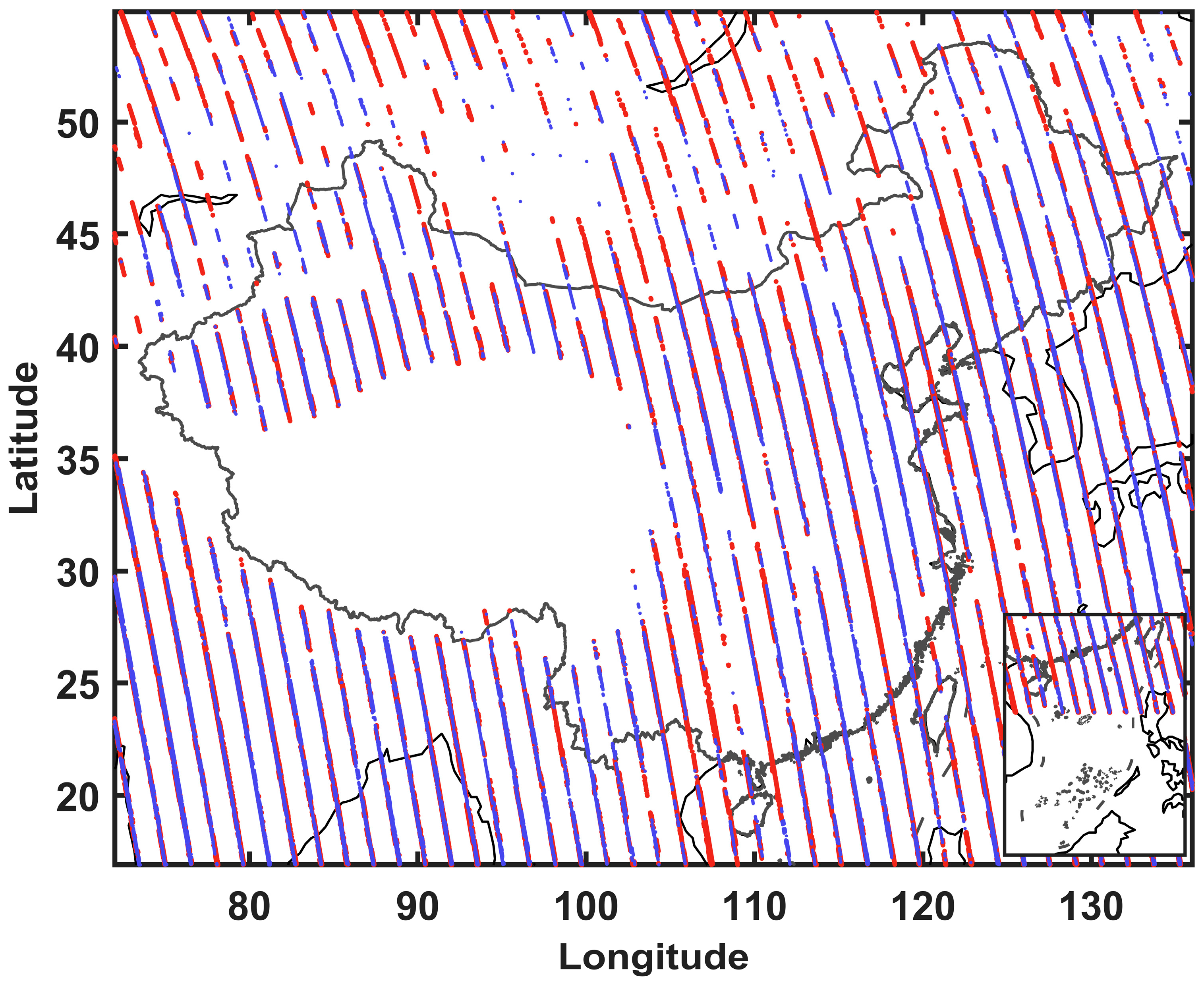
2.1.1. CALIPSO Data
2.1.2. OCO-2 Data
2.2. Methods
2.2.1. Data Processing
2.2.2. Principal Component Analysis
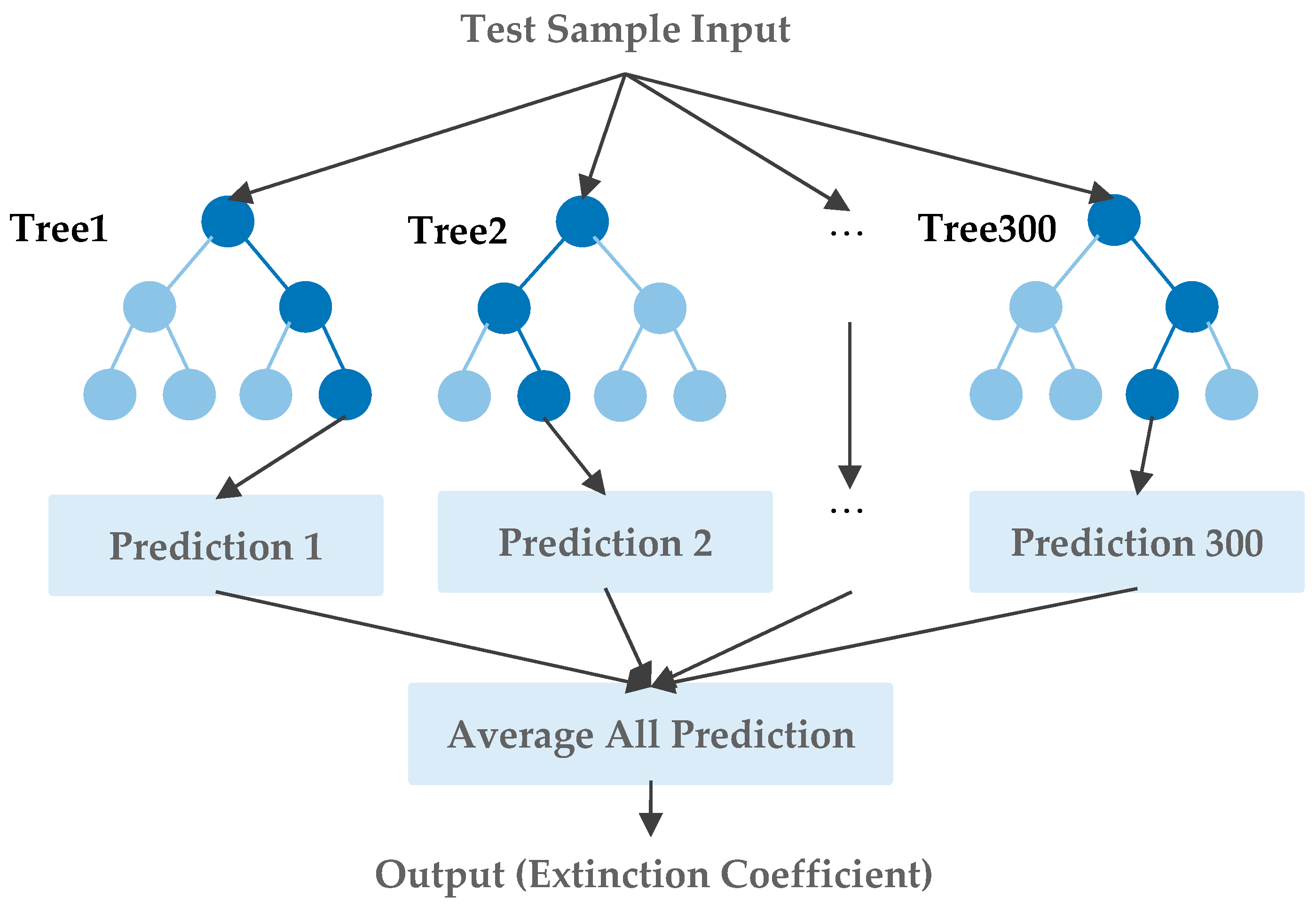
2.2.3. Random Forest Model
2.2.4. Statistical Metrics
3. Results
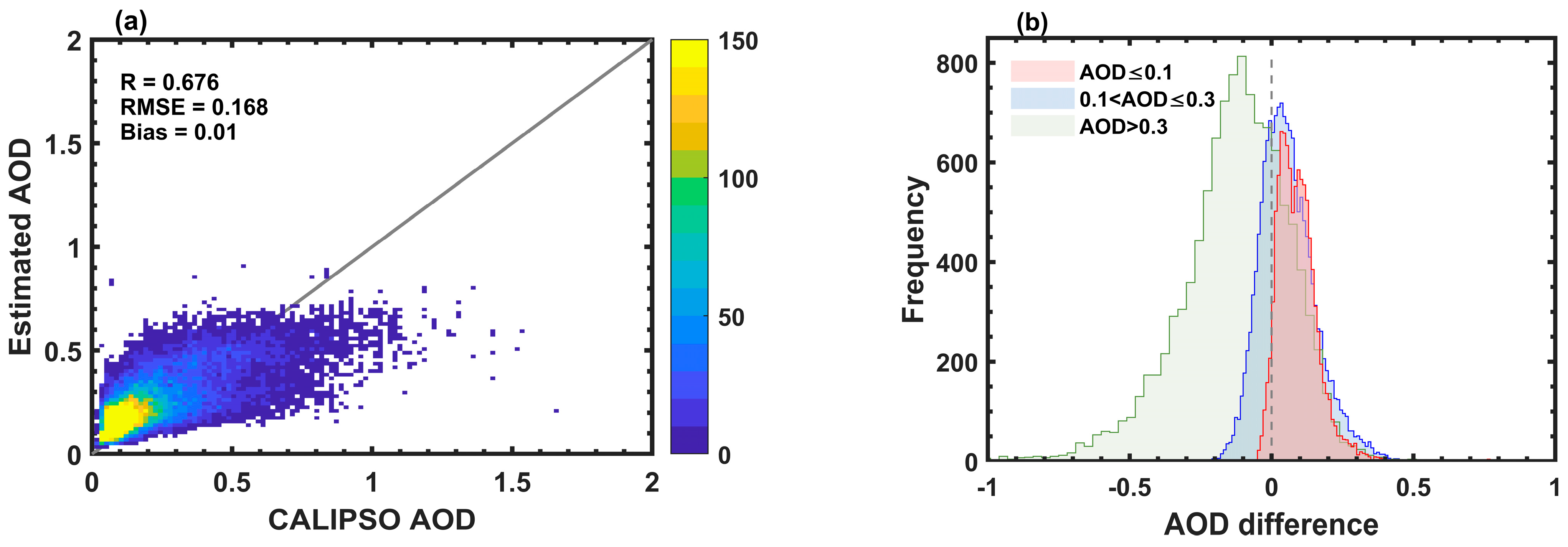
3.1. Evaluation of AOD Accuracy
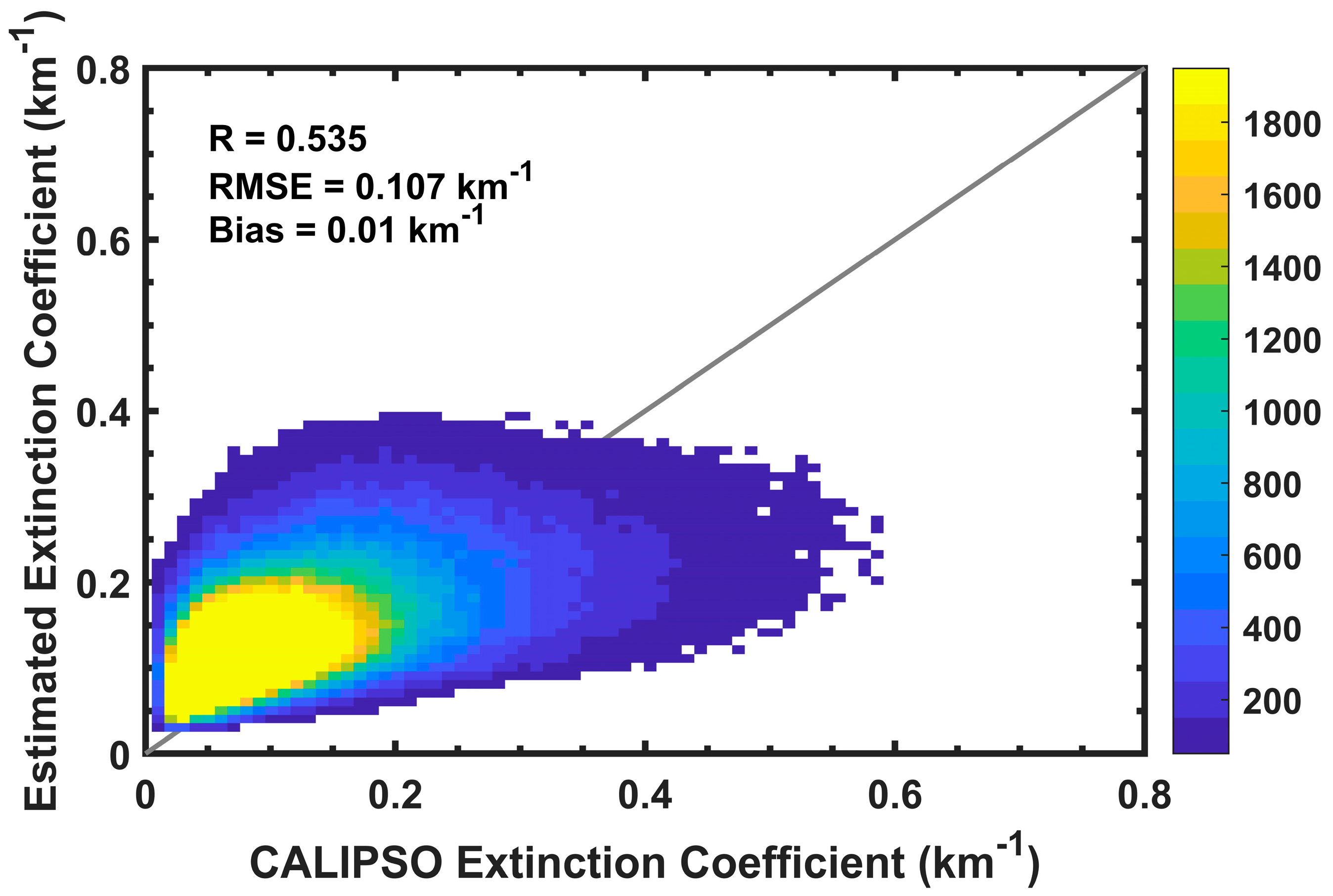
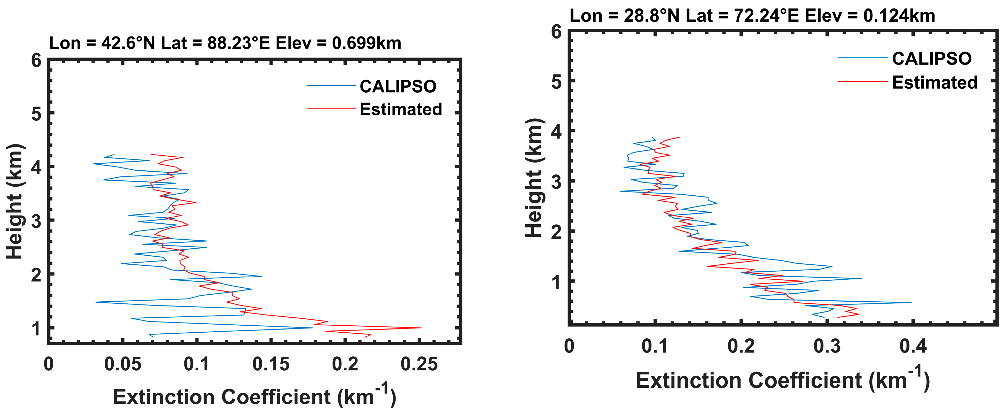
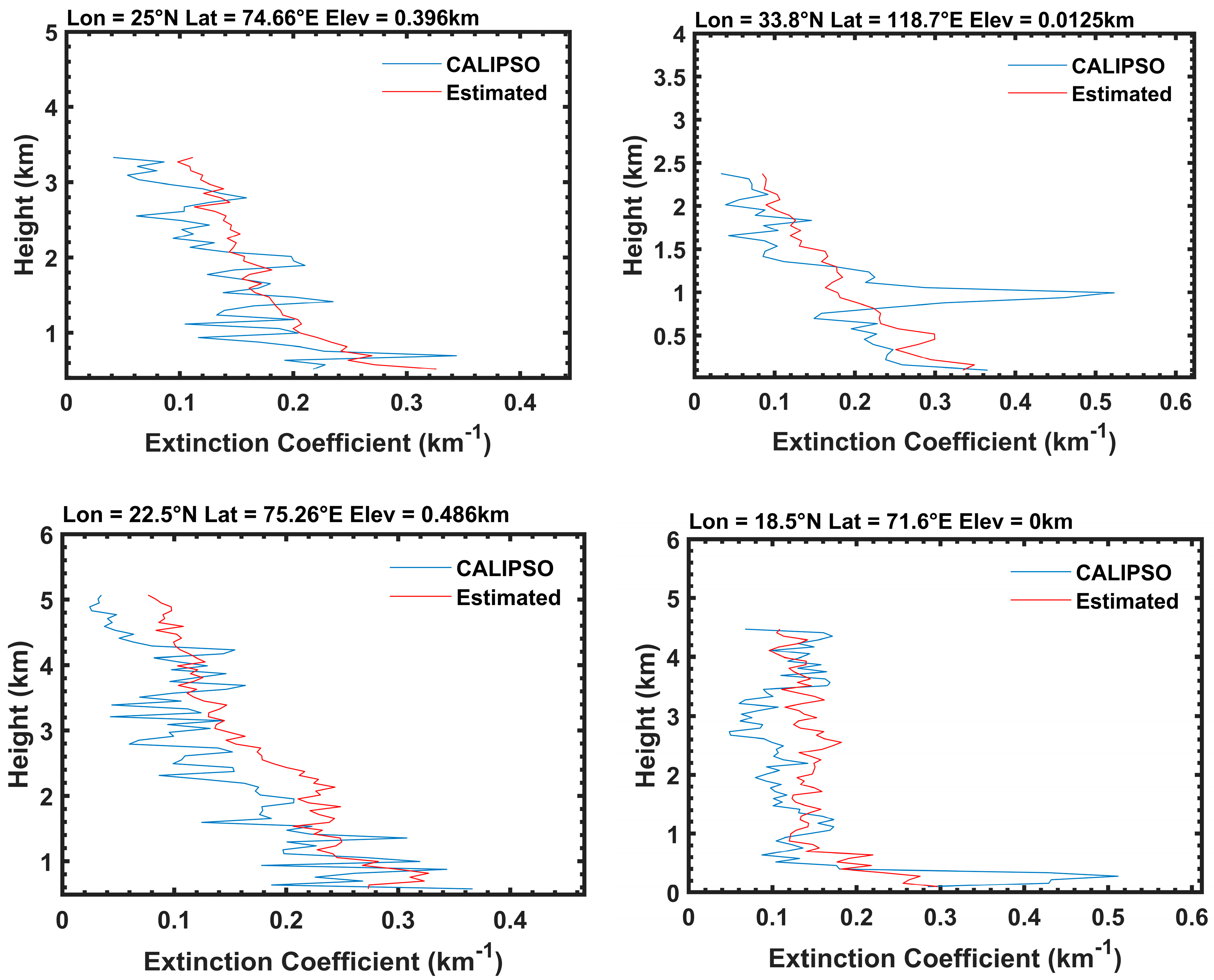
3.2. The Overall Accuracy of Aerosol Profile Retrieval and Assessment at Individual Observation Points
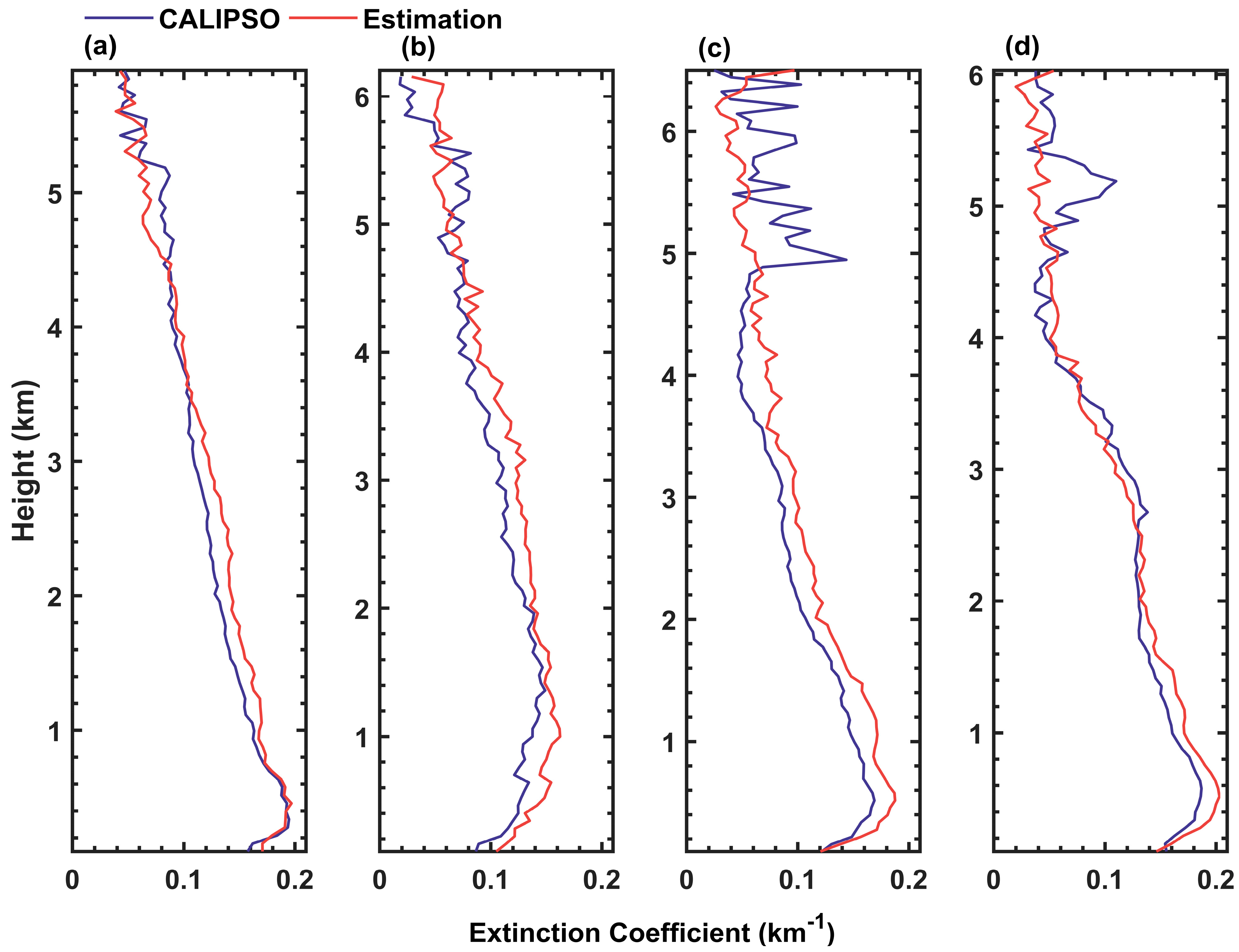
3.3. Seasonal Dependence
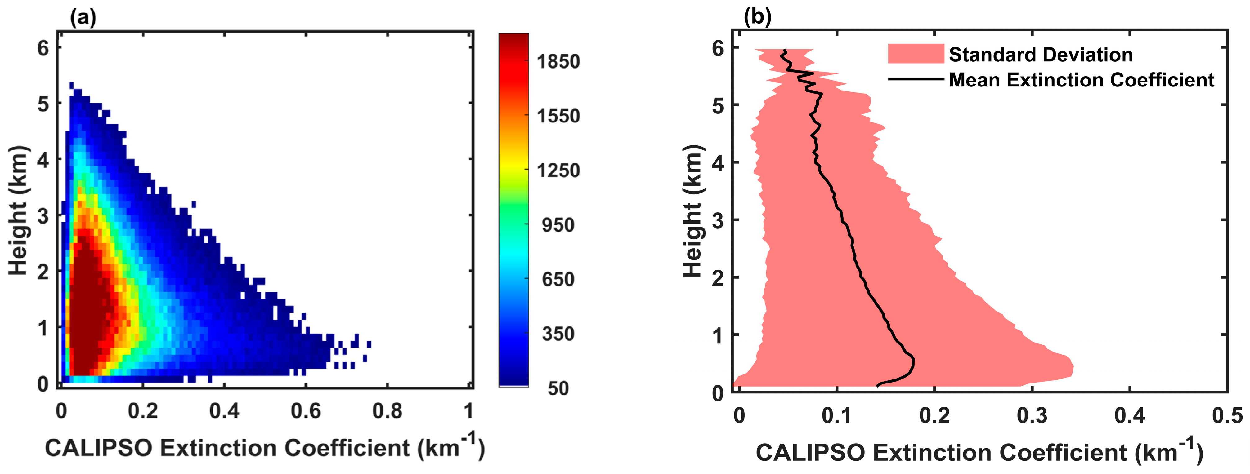
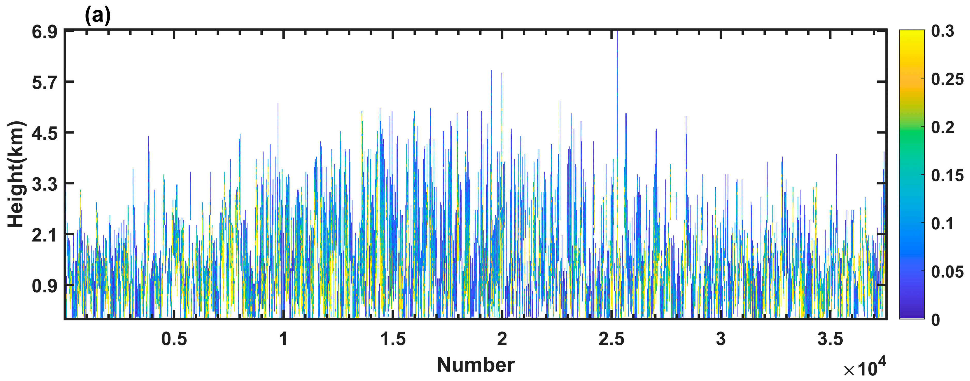
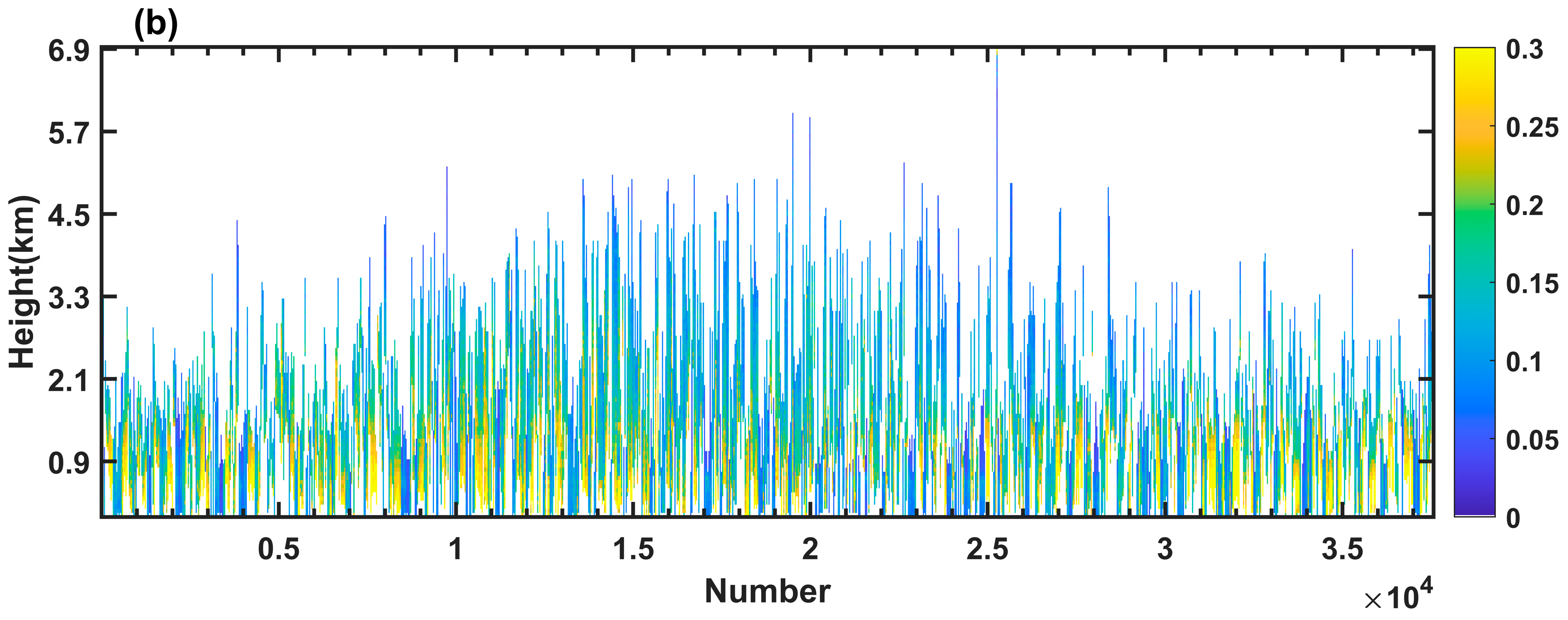
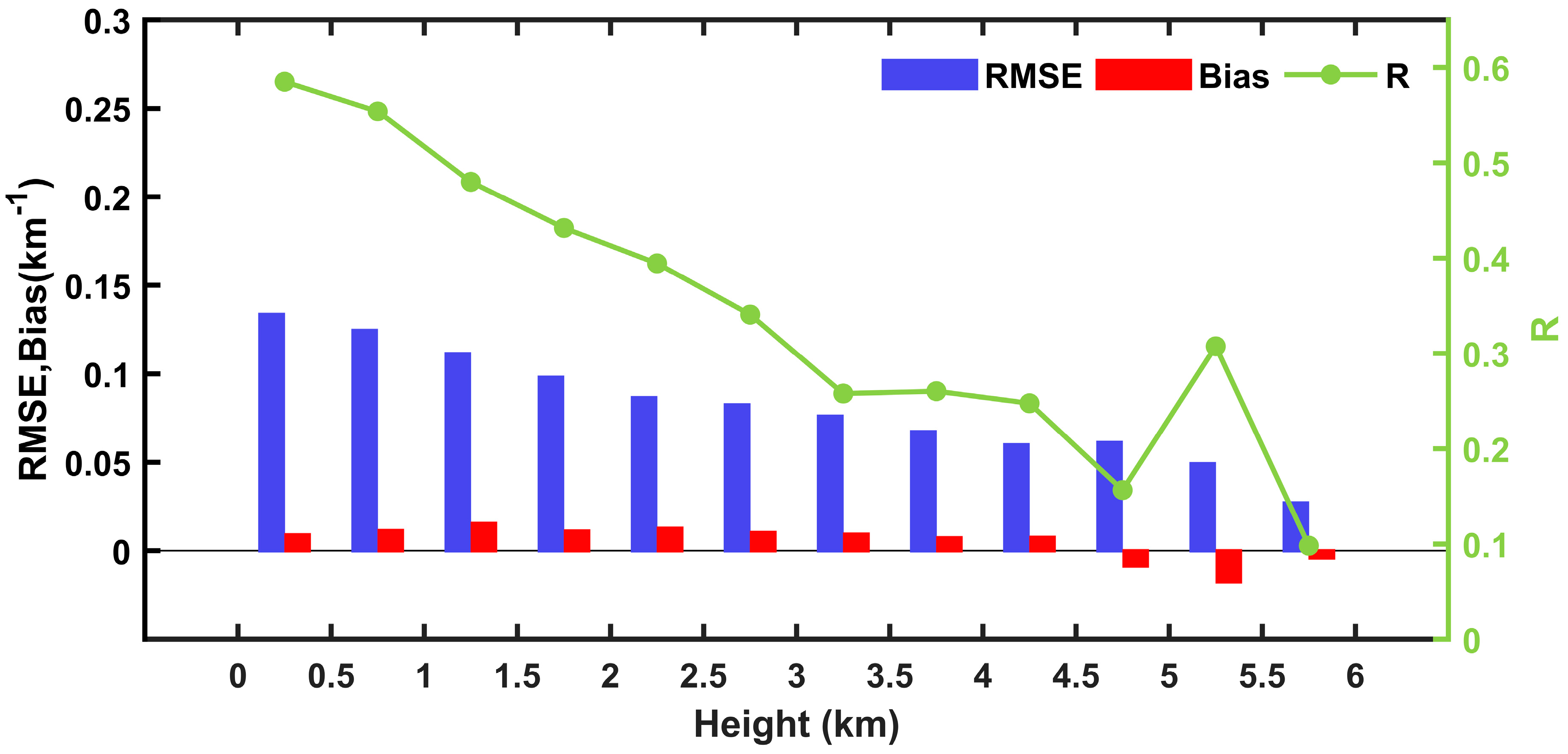
3.4. Height Dependency
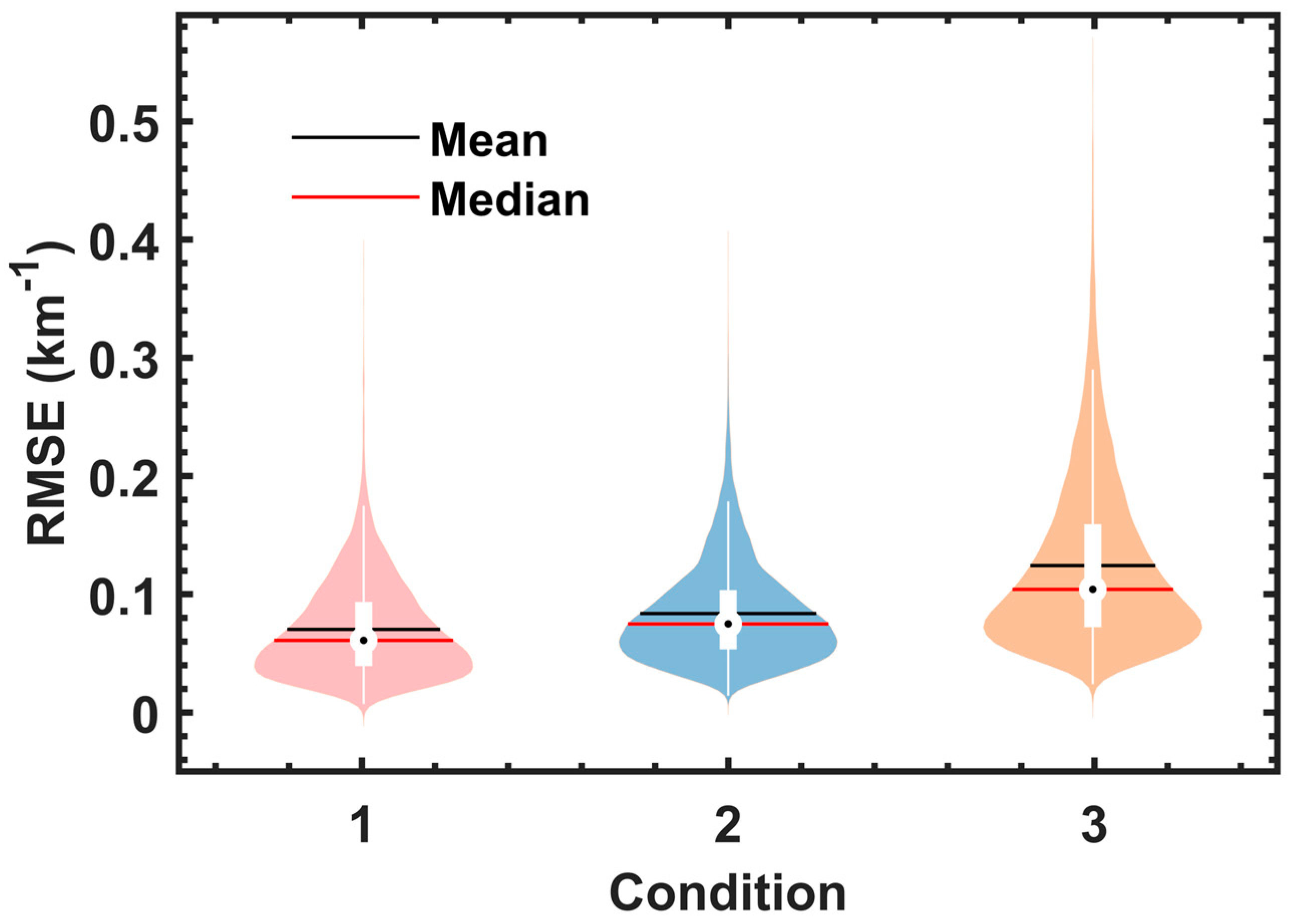
3.5. Accuracy of Aerosol Profile for Different AODs
4. Discussion and Conclusions
Author Contributions
Funding
Data Availability Statement
Acknowledgments
Conflicts of Interest
References
- Ogunkunle, O.; Ahmed, N.A. Overview of Biodiesel Combustion in Mitigating the Adverse Impacts of Engine Emissions on the Sustainable Human-Environment Scenario. Sustainability 2021, 13, 28. [Google Scholar] [CrossRef]
- Baker, E.; Barlow, C.F.; Daniel, L.; Morey, C.; Bentley, R.; Taylor, M.P. Mental health impacts of environmental exposures: A scoping review of evaluative instruments. Sci. Total Environ. 2024, 912, 9. [Google Scholar] [CrossRef] [PubMed]
- Mohan, M.; Payra, S. Influence of aerosol spectrum and air pollutants on fog formation in urban environment of megacity Delhi, India. Environ. Monit. Assess. 2009, 151, 265–277. [Google Scholar] [CrossRef] [PubMed]
- Pöschl, U. Atmospheric Aerosols: Composition, Transformation, Climate and Health Effects. Angew. Chem. Int. Ed. 2006, 44, 7520–7540. [Google Scholar] [CrossRef]
- Shiraiwa, M.; Ueda, K.; Pozzer, A.; Lammel, G.; Kampf, C.J.; Fushimi, A.; Enami, S.; Arangio, A.M.; Fröhlich-Nowoisky, J.; Fujitani, Y.; et al. Aerosol Health Effects from Molecular to Global Scales. Environ. Sci. Technol. 2017, 51, 13545–13567. [Google Scholar] [CrossRef] [PubMed]
- Wang, Y.X.; Sun, X.B.; Huang, H.L.; Ti, R.F.; Liu, X.; Fan, Y.Z. Study on Influencing Factors of the Information Content of Satellite Remote-Sensing Aerosol Vertical Profiles Using Oxygen A-Band. Remote Sens. 2023, 15, 948. [Google Scholar] [CrossRef]
- Charlson, R.J.; Schwartz, S.E.; Hales, J.M.; Cess, R.D.; Coakley, J.A., Jr.; Hansen, J.E.; Hofmann, D.J. Climate forcing by anthropogenic aerosols. Science 1992, 255, 423–430. [Google Scholar] [CrossRef]
- Chen, X.; Wang, J.; Xu, X.G.; Zhou, M.; Zhang, H.X.; Garcia, L.C.; Colarco, P.R.; Janz, S.J.; Yorks, J.; McGill, M.; et al. First retrieval of absorbing aerosol height over dark target using TROPOMI oxygen B band: Algorithm development and application for surface particulate matter estimates. Remote Sens. Environ. 2021, 265, 112674. [Google Scholar] [CrossRef]
- Xue, W.H.; Zhang, J.; Qiao, Y.; Wei, J.; Lu, T.W.; Che, Y.F.; Tian, Y.L. Spatiotemporal variations and relationships of aerosol-radiation-ecosystem productivity over China during 2001–2014. Sci. Total Environ. 2020, 741, 140324. [Google Scholar] [CrossRef]
- Chen, Q.X.; Huang, C.L.; Dong, S.K.; Lin, K.F. Satellite-Based Background Aerosol Optical Depth Determination via Global Statistical Analysis of Multiple Lognormal Distribution. Remote Sens. 2024, 16, 20. [Google Scholar] [CrossRef]
- Cai, H.K.; Yang, Y.; Luo, W.; Chen, Q.L. City-level variations in aerosol optical properties and aerosol type identification derived from long-term MODIS/Aqua observations in the Sichuan Basin, China. Urban Clim. 2021, 38, 100886. [Google Scholar] [CrossRef]
- Zhao, B.; Wang, Y.; Gu, Y.; Liou, K.N.; Jiang, J.H.; Fan, J.W.; Liu, X.H.; Huang, L.; Yung, Y.L. Ice nucleation by aerosols from anthropogenic pollution. Nat. Geosci. 2019, 12, 602–607. [Google Scholar] [CrossRef] [PubMed]
- Bran, S.H.; Jose, S.; Srivastava, R. Investigation of optical and radiative properties of aerosols during an intense dust storm: A regional climate modeling approach. J. Atmos. Sol.-Terr. Phys. 2018, 168, 21–31. [Google Scholar] [CrossRef]
- Andreae, M.O. Natural and anthropogenic aerosols and their effects on clouds, precipitation and climate. Geochim. Cosmochim. Acta 2009, 73, A42. [Google Scholar]
- Wang, F.; Li, Z.Q.; Jiang, Q.; Ren, X.R.; He, H.; Tang, Y.H.; Dong, X.B.; Sun, Y.L.; Dickerson, R.R. Comparative Analysis of Aerosol Vertical Characteristics over the North China Plain Based on Multi-Source Observation Data. Remote Sens. 2024, 16, 1425. [Google Scholar] [CrossRef]
- Nzeffe, F.; Joseph, E.; Min, Q.L. Surface-based observation of aerosol indirect effect in the Mid-Atlantic region. Geophys. Res. Lett. 2008, 35, L22841. [Google Scholar] [CrossRef]
- Jethva, H.; Satheesh, S.K.; Srinivasan, J.; Levy, R.C. Improved retrieval of aerosol size-resolved properties from moderate resolution imaging spectroradiometer over India: Role of aerosol model and surface reflectance. J. Geophys. Res.-Atmos. 2010, 115, D18213. [Google Scholar] [CrossRef]
- Kaufman, Y.J.; Sendra, C. Algorithm for automatic atmospheric corrections to visible and near-IR satellite imagery. Int. J. Remote Sens. 1988, 9, 1357–1381. [Google Scholar] [CrossRef]
- Sinha, P.R.; Nagendra, N.; Manchanda, R.K.; Ojha, D.K.; Kumar, B.S.; Koli, S.K.; Trivedi, D.B.; Lodha, R.K.; Sahu, L.K.; Sreenivasan, S. Development of balloon-borne impactor payload for profiling free tropospheric aerosol. Aerosol Sci. Technol. 2019, 53, 231–243. [Google Scholar] [CrossRef]
- De Tomasi, F.; Perrone, M.R. Lidar measurements of tropospheric water vapor and aerosol profiles over southeastern Italy. J. Geophys. Res.-Atmos. 2003, 108, 4286. [Google Scholar] [CrossRef]
- Chazette, P.; Raut, J.C.; Dulac, F.; Berthier, S.; Kim, S.W.; Royer, P.; Sanak, J.; Loaëc, S.; Grigaut-Desbrosses, H. Simultaneous observations of lower tropospheric continental aerosols with a ground-based, an airborne, and the spaceborne CALIOP lidar system. J. Geophys. Res.-Atmos. 2010, 115, 15. [Google Scholar] [CrossRef]
- Hofmann, D.J. Twenty years of balloon-borne tropospheric aerosol measurements at Laramie, Wyoming. J. Geophys. Res. Atmos. 1993, 98, 12753–12766. [Google Scholar] [CrossRef]
- Deshler, T.; Hofmann, D.J.; Johnson, B.J.; Rozier, W.R. Balloonborne measurements of the Pinatubo aerosol size distribution and volatility at Laramie, Wyoming during the summer of 1991. Geophys. Res. Lett. 2013, 19, 199–202. [Google Scholar] [CrossRef]
- Kiran, V.R.; Ratnam, M.V.; Fujiwara, M.; Russchenberg, H.; Wienhold, F.G.; Madhavan, B.L.; Raman, M.R.; Nandan, R.; Raj, S.T.A.; Kumar, A.H.; et al. Balloon-borne aerosol-cloud interaction studies (BACIS): Field campaigns to understand and quantify aerosol effects on clouds. Atmos. Meas. Tech. 2022, 15, 4709–4734. [Google Scholar] [CrossRef]
- Tegen, I.; Neubauer, D.; Ferrachat, S.; Siegenthaler-Le Drian, C.; Bey, I.; Schutgens, N.; Stier, P.; Watson-Parris, D.; Stanelle, T.; Schmidt, H.; et al. The global aerosol-climate model ECHAM6.3-HAM2.3-Part 1: Aerosol evaluation. Geosci. Model Dev. 2019, 12, 1643–1677. [Google Scholar] [CrossRef]
- Pan, H.L.; Huang, J.P.; An, L.L.; Zhang, J.X.; Kumar, K.R. The CALIPSO retrieved spatiotemporal and vertical distributions of AOD and extinction coefficient for different aerosol types during 2007–2019: A recent perspective over global and regional scales. Atmos. Environ. 2022, 274, 118986. [Google Scholar] [CrossRef]
- He, Y.P.; Xu, X.Q.; Gu, Z.L.; Chen, X.H.; Li, Y.M.; Fan, S.J. Vertical distribution characteristics of aerosol particles over the Guanzhong Plain. Atmos. Environ. 2021, 255, 118444. [Google Scholar] [CrossRef]
- Winker, D.M.; Pelon, J.; Coakley, J.A.; Ackerman, S.A.; Charlson, R.J.; Colarco, P.R.; Flamant, P.; Fu, Q.; Hoff, R.M.; Kittaka, C.; et al. The calipso mission A Global 3D View of Aerosols and Clouds. Bull. Amer. Meteorol. Soc. 2010, 91, 1211–1229. [Google Scholar] [CrossRef]
- Sugimoto, N.; Lee, C.H. Characteristics of dust aerosols inferred from lidar depolarization measurements at two wavelengths. Appl. Opt. 2006, 45, 7468–7474. [Google Scholar] [CrossRef]
- Zeng, Z.L.; Wang, Z.M.; Zhang, B.J. An Adjustment Approach for Aerosol Optical Depth Inferred from CALIPSO. Remote Sens. 2021, 13, 3085. [Google Scholar] [CrossRef]
- Ntwali, D.; Dubache, G.; Ogou, F.K. Vertical Profile Comparison of Aerosol and Cloud Optical Properties in Dominated Dust and Smoke Regions over Africa Based on Space-Based Lidar. Atmos. Clim. Sci. 2022, 12, 588–602. [Google Scholar] [CrossRef]
- Baars, H.; Ansmann, A.; Engelmann, R.; Althausen, D. Continuous monitoring of the boundary-layer top with lidar. Atmos. Chem. Phys. 2008, 8, 7281–7296. [Google Scholar] [CrossRef]
- Mie, G. Beiträge zur Optik trüber Medien, speziell kolloidaler Metallösungen. Ann. Phys. 1908, 330, 377–445. [Google Scholar] [CrossRef]
- Badaev, V.V.; Malkevich, M.S. On the possibility of determining the vertical profiles of aerosol attenuation using satellite measurements of reflected radiation in the 0.76 micron oxygen band. Akad. Nauk. SSSR Fiz. Atmos. Okeana 1979, 14, 1022–1030. [Google Scholar]
- Gabella, M.; Guzzi, R.; Kisselev, V.; Perona, G. Retrieval of aerosol profile variations in the visible and near infrared: Theory and application of the single-scattering approach. Appl. Opt. 1997, 36, 1328–1336. [Google Scholar] [CrossRef] [PubMed]
- Corradini, S.; Cervino, M. Aerosol extinction coefficient profile retrieval in the oxygen A-band considering multiple scattering atmosphere. J. Quant. Spectrosc. Radiat. Transf. 2006, 97, 354–380. [Google Scholar] [CrossRef]
- Malladi, S.; Radha, R.S.; Pillai, V.P.M.; Sangipillai, V.; Bhargavan, P.; Vinjanampaty, M.; Karnam, R. Laser radar characterization of atmospheric aerosols in the troposphere and stratosphere using range dependent lidar ratio. J. Appl. Remote Sens. 2010, 4, 20. [Google Scholar] [CrossRef]
- Oo, M.; Holz, R. Improving the CALIOP aerosol optical depth using combined MODIS-CALIOP observations and CALIOP integrated attenuated total color ratio. J. Geophys. Res.-Atmos. 2011, 116, D14201. [Google Scholar] [CrossRef]
- Yan, Z.; Minzheng, D.; Daren, L. Retrieving aerosol extinction profile with high spectral resolution radiance in Oxygen A-band and Simulation research. Remote Sens. Technol. Appl. 2012, 27, 208–219. [Google Scholar]
- Sanders, A.F.J.; de Haan, J.F. Retrieval of aerosol parameters from the oxygen A band in the presence of chlorophyll fluorescence. Atmos. Meas. Tech. 2013, 6, 2725–2740. [Google Scholar] [CrossRef]
- Geddes, A.; Bösch, H. Tropospheric aerosol profile information from high-resolution oxygen A-band measurements from space. Atmos. Meas. Tech. 2015, 8, 859–874. [Google Scholar] [CrossRef]
- Ding, S.G.; Wang, J.; Xu, X.G. Polarimetric remote sensing in oxygen A and B bands: Sensitivity study and information content analysis for vertical profile of aerosols. Atmos. Meas. Tech. 2016, 9, 2077–2092. [Google Scholar] [CrossRef]
- Zeng, Z.C.; Chen, S.; Natraj, V.; Le, T.; Xu, F.; Merrelli, A.; Crisp, D.; Sander, S.P.; Yung, Y.L. Constraining the vertical distribution of coastal dust aerosol using OCO-2 O2 A-band measurements. Remote Sens. Environ. 2020, 236, 111494. [Google Scholar] [CrossRef]
- Chen, S.H.; Natraj, V.; Zeng, Z.C.; Yung, Y.L. Machine learning-based aerosol characterization using OCO-2 O2 A-band observations. J. Quant. Spectrosc. Radiat. Transf. 2022, 279, 108049. [Google Scholar] [CrossRef]
- L’Ecuyer, T.S. Touring the atmosphere aboard the A-Train. Phys. Today 2011, 64, 245–256. [Google Scholar]
- Meng, F.; Cao, C.Y.; Shao, X. Spatio-temporal variability of Suomi-NPP VIIRS-derived aerosol optical thickness over China in 2013. Remote Sens. Environ. 2015, 163, 61–69. [Google Scholar] [CrossRef]
- Natraj, V.; Spurr, R.J.D.; Boesch, H.; Jiang, Y.B.; Yung, Y.L. Evaluation of errors from neglecting polarization in the forward modeling of O2 A band measurements from space, with relevance to CO2 column retrieval from polarization-sensitive instruments. J. Quant. Spectrosc. Radiat. Transf. 2007, 103, 245–259. [Google Scholar] [CrossRef]
- Shikwambana, L.; Sivakumar, V. Global distribution of aerosol optical depth in 2015 using CALIPSO level 3 data. J. Atmos. Sol.-Terr. Phys. 2018, 173, 150–159. [Google Scholar] [CrossRef]
- Pan, B.W.; Liu, D.T.; Kumar, K.R.; Wang, M.; Devi, N. Global distribution of maritime low clouds with an emphasis on different aerosol types and meteorological parameters inferred from multi-satellite and reanalysis data during 2007–2016. Atmos. Environ. 2021, 246, 118082. [Google Scholar] [CrossRef]
- Nanda, S.; de Graaf, M.; Veefkind, J.P.; Sneep, M.; ter Linden, M.; Sun, J.Y.T.; Levelt, P.F. A first comparison of TROPOMI aerosol layer height (ALH) to CALIOP data. Atmos. Meas. Tech. 2020, 13, 3043–3059. [Google Scholar] [CrossRef]
- Mehta, M.; Singh, N.; Anshumali. Global trends of columnar and vertically distributed properties of aerosols with emphasis on dust, polluted dust and smoke—Inferences from 10-year long CALIOP observations. Remote Sens. Environ. 2018, 208, 120–132. [Google Scholar] [CrossRef]
- Wang, F.; Guo, J.P.; Zhang, J.H.; Huang, J.F.; Min, M.; Chen, T.M.; Liu, H.; Deng, M.J.; Li, X.W. Multi-sensor quantification of aerosol-induced variability in warm clouds over eastern China. Atmos. Environ. 2015, 113, 1–9. [Google Scholar] [CrossRef]
- Eldering, A.; Wennberg, P.O.; Crisp, D.; Schimel, D.S.; Gunson, M.R.; Chatterjee, A.; Liu, J.; Schwandner, F.M.; Sun, Y.; O’Dell, C.W.; et al. The Orbiting Carbon Observatory-2 early science investigations of regional carbon dioxide fluxes. Science 2017, 358, eaam5745. [Google Scholar] [CrossRef] [PubMed]
- O’Dell, C.W.; Eldering, A.; Wennberg, P.O.; Crisp, D.; Gunson, M.R.; Fisher, B.; Frankenberg, C.; Kiel, M.; Lindqvist, H.; Mandrake, L.; et al. Improved retrievals of carbon dioxide from Orbiting Carbon Observatory-2 with the version 8 ACOS algorithm. Atmos. Meas. Tech. 2018, 11, 6539–6576. [Google Scholar] [CrossRef]
- Richardson, M.; Lebsock, M.D.; McDuffie, J.; Stephens, G.L. A new Orbiting Carbon Observatory 2 cloud flagging method and rapid retrieval of marine boundary layer cloud properties. Atmos. Meas. Tech. 2020, 13, 4947–4961. [Google Scholar] [CrossRef]
- Liu, X.; Smith, W.L.; Zhou, D.K.; Larar, A. Principal component-based radiative transfer model for hyperspectral sensors: Theoretical concept. Appl. Opt. 2006, 45, 201–209. [Google Scholar] [CrossRef] [PubMed]
- Liu, X.; Yang, Q.G.; Li, H.; Jin, Z.H.; Wu, W.; Kizer, S.; Zhou, D.K.; Yang, P. Development of a fast and accurate PCRTM radiative transfer model in the solar spectral region. Appl. Opt. 2016, 55, 8236–8247. [Google Scholar] [CrossRef] [PubMed]
- Breiman, L. Random forests. Mach. Learn. 2001, 45, 5–32. [Google Scholar] [CrossRef]
- Huang, Y.; Bao, Y.S.; Petropoulos, G.P.; Lu, Q.F.; Huo, Y.F.; Wang, F. Precipitation Estimation Using FY-4B/AGRI Satellite Data Based on Random Forest. Remote Sens. 2024, 16, 1267. [Google Scholar] [CrossRef]
- Zhu, W.D.; Li, Y.Q.; Luan, K.F.; Qiu, Z.E.; He, N.Y.; Zhu, X.L.; Zou, Z.Y. Forest Canopy Height Retrieval and Analysis Using Random Forest Model with Multi-Source Remote Sensing Integration. Sustainability 2024, 16, 1735. [Google Scholar] [CrossRef]
- Zhang, L.; Wang, X.; Huang, G.; Zhang, S. Comprehensive Assessment and Analysis of the Current Global Aerosol Optical Depth Products. Remote Sens. 2024, 16, 1425. [Google Scholar] [CrossRef]
- Sun, T.Z.; Che, H.Z.; Qi, B.; Wang, Y.Q.; Dong, Y.S.; Xia, X.G.; Wang, H.; Gui, K.; Zheng, Y.; Zhao, H.J.; et al. Characterization of vertical distribution and radiative forcing of ambient aerosol over the Yangtze River Delta during 2013–2015. Sci. Total Environ. 2019, 650, 1846–1857. [Google Scholar] [CrossRef] [PubMed]

| Principal Components | Eigenvalues | Contribution Rate (%) | Cumulative Contribution Rate (%) |
|---|---|---|---|
| 1 | 3.0777 × 10⁴ | 98.4594 | 98.4594 |
| 2 | 343.7895 | 1.0998 | 99.5592 |
| 3 | 97.7374 | 0.3127 | 99.8719 |
| 4 | 15.7895 | 0.0505 | 99.9224 |
| 5 | 10.8076 | 0.0346 | 99.9570 |
| 6 | 5.5176 | 0.0177 | 99.9747 |
| 7 | 2.9030 | 0.0093 | 99.9840 |
| 8 | 1.9107 | 0.0061 | 99.9901 |
| 9 | 0.9865 | 0.0032 | 99.9933 |
| 10 | 0.3768 | 0.0012 | 99.9945 |
| 11 | 0.2533 | 8.1043 × 10⁻⁴ | 99.9953 |
| … | … | … | … |
| Season | R | RMSE (km−1) | Bias (km−1) |
|---|---|---|---|
| Spring | 0.535 | 0.102 | 0.009 |
| Summer | 0.442 | 0.101 | 0.014 |
| Autumn | 0.557 | 0.107 | 0.017 |
| Winter | 0.527 | 0.115 | 0.010 |
Disclaimer/Publisher’s Note: The statements, opinions and data contained in all publications are solely those of the individual author(s) and contributor(s) and not of MDPI and/or the editor(s). MDPI and/or the editor(s) disclaim responsibility for any injury to people or property resulting from any ideas, methods, instructions or products referred to in the content. |
© 2024 by the authors. Licensee MDPI, Basel, Switzerland. This article is an open access article distributed under the terms and conditions of the Creative Commons Attribution (CC BY) license (https://creativecommons.org/licenses/by/4.0/).
Share and Cite
Zhou, X.-Q.; Liu, H.-L.; Duan, M.-Z.; Chen, B.; Zhang, S.-L. Random Forest Model-Based Inversion of Aerosol Vertical Profiles in China Using Orbiting Carbon Observatory-2 Oxygen A-Band Observations. Remote Sens. 2024, 16, 2497. https://doi.org/10.3390/rs16132497
Zhou X-Q, Liu H-L, Duan M-Z, Chen B, Zhang S-L. Random Forest Model-Based Inversion of Aerosol Vertical Profiles in China Using Orbiting Carbon Observatory-2 Oxygen A-Band Observations. Remote Sensing. 2024; 16(13):2497. https://doi.org/10.3390/rs16132497
Chicago/Turabian StyleZhou, Xiao-Qing, Hai-Lei Liu, Min-Zheng Duan, Bing Chen, and Sheng-Lan Zhang. 2024. "Random Forest Model-Based Inversion of Aerosol Vertical Profiles in China Using Orbiting Carbon Observatory-2 Oxygen A-Band Observations" Remote Sensing 16, no. 13: 2497. https://doi.org/10.3390/rs16132497
APA StyleZhou, X.-Q., Liu, H.-L., Duan, M.-Z., Chen, B., & Zhang, S.-L. (2024). Random Forest Model-Based Inversion of Aerosol Vertical Profiles in China Using Orbiting Carbon Observatory-2 Oxygen A-Band Observations. Remote Sensing, 16(13), 2497. https://doi.org/10.3390/rs16132497