High-Resolution PM₁₀ Estimation Using Satellite Data and Model-Agnostic Meta-Learning

Abstract

Characterizing the spatial distribution of particles smaller than 10 μm (PM₁₀) is of great importance for air quality management yet is very challenging because of the sparseness of air quality monitoring stations. In this study, we use a model-agnostic meta-learning-trained artificial neural network (MAML-ANN) to estimate the concentrations of PM₁₀ at 60 m × 60 m spatial resolution by combining satellite-derived aerosol optical depth (AOD) with meteorological data. The network is designed to regress from the predictors at a specific time to the ground-level PM₁₀ concentration. We utilize the ANN model to capture the time-specific nonlinearity among aerosols, meteorological conditions, and PM₁₀, and apply MAML to enable the model to learn the nonlinearity across time from only a small number of data samples. MAML is also employed to transfer the knowledge learned from coarse spatial resolution to high spatial resolution. The MAML-ANN model is shown to accurately estimate high-resolution PM₁₀ in Beijing, with coefficient of determination of 0.75. MAML improves the PM₁₀ estimation performance of the ANN model compared with the baseline using pre-trained initial weights. Thus, MAML-ANN has the potential to estimate particulate matter estimation at high spatial resolution over other data-sparse, heavily polluted, and small regions.

1. Introduction

Coarse particulate matter with a diameter of 10 μm or less (PM₁₀), usually given in ${\mu \mathrm{g}/\mathrm{m}}^3$, are tightly linked with emphysema, diabetes, and hypertension [1,2], and is globally responsible for a large number of premature deaths [3,4]. Although discussions on effective measures to reduce PM concentrations are ongoing, the main factors in pollutant distribution are still a matter of debate [5,6]. In order to better protect the public from excessive exposure to particulate matter, characterizing the spatial distribution of PM₁₀ is necessary. However, networks of air pollutant monitoring stations are often not dense enough to characterize the high spatial variability of PM, limiting the improvement of effective measures toward better air quality. Thus, novel and low-cost solutions to map PM at high spatial resolution are critically in demand.

Satellite remote sensing is a potentially useful tool for monitoring air pollution with high spatiotemporal resolution, especially in areas where ground measurements are sparse or not available [6,7]. Aerosol optical depth (AOD), defined as the radiation extinction by aerosol in an atmospheric column at a certain wavelength [8], is the most applicable satellite-retrieved product for estimating PM concentrations [9]. A vast number of studies have used satellite-derived AOD observations to indicate ground-level air pollutant. For example, Gupta et al. made use of moderate resolution imaging spectroradiometer (MODIS)-derived AOD to estimate surface level PM_2.5 mass concentration [10]. Lee et al. also predicted ground daily PM_2.5 concentrations based on MODIS AOD data [9]. You et al. utilized satellite AOD to improve the estimation accuracy of ground-level PM₁₀ from geographically weighted regression (GWR) model [11].

Meteorological conditions play a considerable role in quantifying the AOD-PM relationship and have been widely used as auxiliary predictors in many PM predictive models [10,12]. Stirnberg et al. combined the satellite-borne AOD with meteorological parameters to predict hourly concentrations of PM₁₀ in Germany [6]. Hu et al. found that the combination of AOD, meteorological parameters, and land use information can lead the GWR model to estimate PM_2.5 more accurately [13]. Koelemeijer et al. improved the correlation between PM and AOD by introducing meteorological conditions, allowing for better monitoring of PM distributions via satellite AOD measurements [14].

Artificial neural networks (ANNs) have become increasingly prevalent in modeling a wide range of air pollutants distribution due to their nonlinear feature mapping and computational efficiency [15,16]. Cermak et al. built an ANN model to relate AOD to meteorological conditions and then predicted the 2008 AOD by using the meteorological observations of that year [17]. Perez et al. presented a PM₁₀ forecasting model that integrated the ANN with a nearest neighbor model (NNM) to manage the air quality in Santiago, Chile [18]. On the basis of an ANN model, Park et al. predicted the indoor PM concentration of subway systems in Seoul by coupling the information of outdoor PM with the number of subway trains running and information on ventilation operation [19]. Although ANNs have been used as a tool for air pollutant prediction with varying success, they have challenges in mapping PM distributions at high spatial resolution. The prediction accuracy of ANNs essentially depends on the amount of input observation data. However, current available satellite AOD products are at several to tens of kilometers resolution, constraining the satellite-retrieved PM to a coarse spatial resolution. By taking advantage of high-resolution satellite measurements, such as Landsat-7, Landsat-8, or Sentinel-2, several studies have developed aerosol retrieval algorithms to generate AODs at a spatial resolution of 500 m × 500 m or higher [20,21,22]. Unfortunately, the acquisition of sufficient high-resolution satellite AOD remains difficult in many cases, limiting the supervised machine learning model to predict PM accurately without overfitting. To ensure the retrieval accuracy, most aerosol retrieval algorithms use strict cloud filtering and will not be applied to non-eligible products. In addition, the full operation of high-resolution aerosol retrieval algorithms globally still takes effort.

Meta-learning can help models solve few-shot problems, providing great promise for models to learn from a limited number of examples [23,24]. The mechanism of meta-learning is to train the model to be able to learn how to learn through experiencing a variety of different tasks (known as “learning to learn”), such that the trained model can quickly learn a new task from only a few examples [25]. Recently, a state-of-the-art meta-learning algorithm, i.e., the model-agnostic meta-learning (MAML) algorithm, was proposed by Finn et al. to favor the model to easily handle different few-shot problems without constrains on model architecture [26]. Subsequently, Rußwurm et al. explored MAML for remote sensing applications and demonstrated that MAML optimization is able to improve the land cover classification accuracy of convolution neural networks (CNNs) across geographies [27]. Tseng et al. also exerted MAML to enable a long short-term memory (LSTM) model to effectively learn from many heterogeneous datasets and then predicted the crop type in satellite observations of label-sparse regions [25].

Monitoring air pollution in small and local regions can greatly benefit policymakers in formulating PM₁₀ control measures yet is very challenging. Currently, few studies have mapped PM at high spatial resolution. In this study, we view the high-resolution PM₁₀ estimation task as one meta-learning problem and make use of MAML to tackle (1) the complex spatial correlations between stations; (2) the time-varying relationship among aerosol, meteorological conditions, and PM₁₀; and (3) the scarcity of high-resolution satellite AOD products. Commonly, PM_2.5 is more closely associated with human morbidity and mortality than PM₁₀ [28]. However, PM_2.5 excludes the fraction of larger particles, which are nevertheless accountable for light extinction and thus contribute to AOD measured by the satellite [6]. Therefore, the focus of this study is on PM₁₀ instead. The ANN model with one hidden layer serves as the regressor to handle the time-specific PM₁₀ estimation task by incorporating satellite AOD observations with meteorological information. We conduct a case study in Beijing over a period of ~7 years from 2013 to 2019. To evaluate the PM₁₀ estimation performance of the proposed methodology, we further compare the estimations of the MAML-trained ANN (MAML-ANN) model with a pre-trained ANN (P-ANN) model.

Details of the data used in the study area are described in Section 2. Section 3 introduces the proposed methodology. Section 4 shows the validation results against the ground measurements. Section 5 elaborates the comparison results with the baseline and competitors. Conclusions are summarized in Section 6.

2. Materials

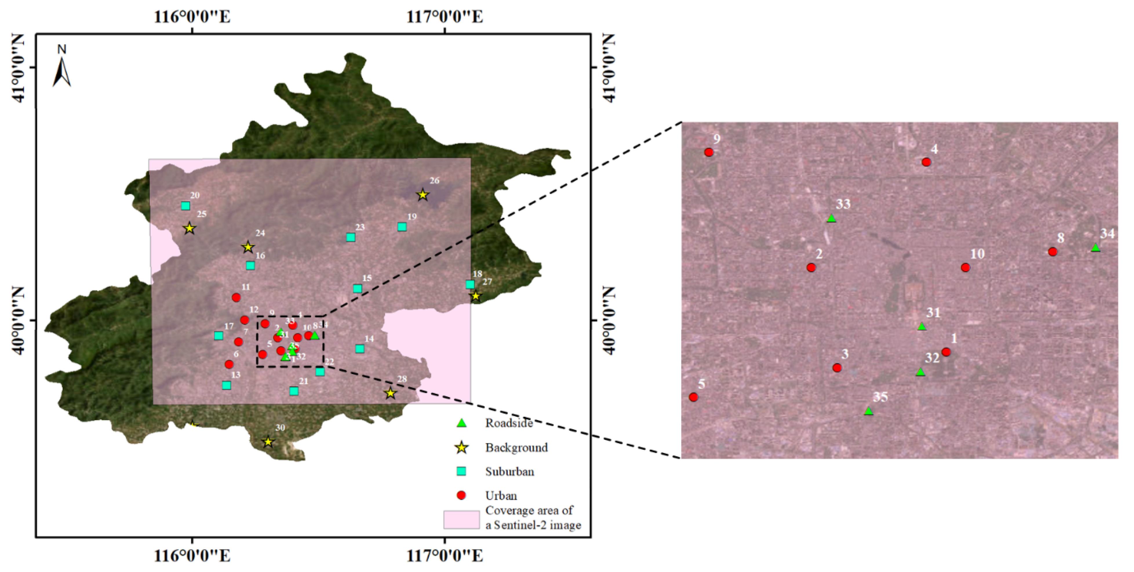
2.1. Ground-based PM₁₀ Data

Beijing is set in a heavily industrialized and urbanized region with notoriously high and variable particulate matter pollution [17,29]. To strengthen the monitoring of ambient air pollution, a total of 35 regulatory air quality monitoring stations are installed in the area and maintained by the Beijing Municipal Environmental Protection Bureau (BJEPB) [30]. The distributions of these 35 stations are provided in Figure 1, along with the corresponding names, coordinates, and station types being tabulated in

Table 1. Details of the 35 air quality monitoring stations in Beijing.

Number	Name	Longitude	Latitude	Type
1	Temple of Heaven	116.407	39.886	Urban
2	Guanyuan	116.339	39.929	Urban
3	Wanshou Palace	116.352	39.878	Urban
4	Olympic Sports Center	116.397	39.982	Urban
5	Fengtai Garden	116.279	39.863	Urban
6	Yungang	116.146	39.824	Urban
7	Gucheng	116.184	39.914	Urban
8	Nongzhanguan	116.461	39.937	Urban
9	Wanliu	116.287	39.987	Urban
10	Dongsi	116.417	39.929	Urban
11	New North Zone	116.174	40.09	Urban
12	Botanical Garden	116.207	40.002	Urban
13	Fangshan	116.136	39.742	Suburban
14	Tongzhou	116.663	39.886	Suburban
15	Shunyi	116.655	40.127	Suburban
16	Changping	116.23	40.217	Suburban
17	Mentougou	116.106	39.937	Suburban
18	Pinggu	117.1	40.143	Suburban
19	Miyun	116.832	40.37	Suburban
20	Yanqing	115.972	40.453	Suburban
21	Daxing	116.404	39.718	Suburban
22	Yizhuang	116.506	39.795	Suburban
23	Huairou	116.628	40.328	Suburban
24	Dingling	116.22	40.292	Background
25	Badaling	115.988	40.365	Background
26	Miyun Reservior	116.911	40.499	Background
27	Donggaocun	117.12	40.1	Background
28	Yongledain	116.783	39.712	Background
29	Liulihe	116	39.58	Background
30	Yufa	116.3	39.52	Background
31	Qianmen	116.395	39.899	Roadside
32	Yongdingmennei	116.394	39.876	Roadside
33	Xizhibeimen	116.349	39.954	Roadside
34	East 4th Ring Road	116.483	39.939	Roadside
35	South 3rd Ring Road	116.368	39.856	Roadside

. Stations are designed to be representative of a variety of different types of areas and can be classified as urban, suburban, background, or roadside.

In this study, a small rectangular area (equal to the area covered by a Sentinel-2 image) around Beijing is selected as the test bed for validating the proposed method. The hourly PM₁₀ concentration data from the 32 stations (Donggao Village, Yuzhan, and Liuli River stations are not covered by the Sentinel-2 image) are used as labels for the period between 2013 and 2019. Coordinates of the PM₁₀ stations are employed as spatial reference for data collocation, that is, pixels from satellite and reanalysis images are collocated with the same positions of the ground-based stations. In order to increase the number of PM₁₀ observations, we substitute the missing concentrations with corresponding daily mean if at least three hourly observations on that day are available. Localized events may lead to anomalous observed PM₁₀ concentrations, affecting the estimation accuracy of the proposed model seriously. Thus, a boxplot is adopted to filter out the extreme outliers (outside the outer fence = 3 × interquartile range (IQR)) in collected PM₁₀ concentrations.

2.2. Satellite Data

AOD is an important input to the model, as it provides implicit information on atmospheric particle concentrations [31]. In this study, we make use of the 60 m × 60 m AOD derived from Sentinel-2 measurements from 2017 to 2019 by application of the Yang et al. algorithm to compute the ground-level PM₁₀ concentrations at high spatial resolution [32]. Yang et al. make use of the surface reflectance correlations with a combination of temporal signatures over the vegetated areas and bright areas to retrieve the 60 m by 60 m AOD from Sentinel-2 Level-1C (L1C). The data quality of the used Sentinel-2 AOD is demonstrated to be reliable (correlation coefficient of 0.927 to ground-based AOD measurements) and has been successfully applied to characterize the spatiotemporal patterns of AOD over Beijing [8]. Sentinel-2 overpass time over Beijing (around ~3 UTC) is taken as the temporal reference for data collocation. Because other model features (i.e., ground-based PM₁₀ and meteorological data) are released hourly, ~3 UTC is used as the valid reference time to simplify data collocation.

We should note that the Sentinel-2 mission (i.e., Sentinel-2A/B) was launched in 2017 and only has a temporal resolution of 5 days. Thus, the quantity of Sentinel-2 AOD is too sparse to train the model without overfitting. To solve this problem, the high temporal resolution AOD product sourced from MODIS covering four years (2013–2016) is introduced in the absence of Sentinel-2 AOD. Currently, MODIS aerosol products are released at three spatial resolutions: 1 km × 1 km, 3 km × 3 km, and 10 km × 10 km. The fine-resolution AOD product (i.e., 1 km × 1 km MCD19A2) seems to be the optimal substitute. However, its daily resolution prevents it from temporally matching with other input data with hourly resolution. Therefore, the 10 km × 10 km resolution MOD04_L2 AOD products with acquisition times ranging from ~1 to ~5 UTC are selected instead due to their higher precision and more available retrievals than the 3 km × 3 km AOD products [33,34]. Furthermore, only the recommended high-quality dark target and deep blue combined (variable name: AOD_550_Dark_Target_Deep_Blue_Combined) AOD retrievals are used [35]. The correlation coefficient between the used Sentinel-2 AOD and MOD04_L2 AOD is of 0.92, suggesting that the particle field is fairly uniform across tens of kilometers. Therefore, it is reasonable to use MOD04_L2 AOD in the absence of Sentinel-2 AOD.

2.3. Meteorological Data

Meteorology substantially influences the concentrations of atmospheric particulate matter [10]. Incorporating meteorological conditions into PM predictive models not only contributes to a more reasonable AOD-PM relationship, but also benefits the estimation of abrupt changes in ground-level particle concentrations [6,36]. To represent the meteorological conditions in the study area, ERA5-Land hourly reanalysis data generated by the European Centre for Medium-Range Weather Forecasts (ECMWF) for the whole study period with a spatial resolution of 0.1° and a release time of ~3 UTC are employed [37]. Specifically, wind components in eastward and northward at a height of 10 m above the surface of the Earth, wind direction calculated from the two wind components, air temperature at 2 m height, and atmospheric pressure are included as the meteorological predictors of the proposed PM₁₀ estimation model. The wind regulates particle transport and greatly modifies PM₁₀ concentrations [6,38]. Temperature impacts the particle number in the atmosphere by stimulating photochemical reactions [10]. For instance, high temperature transforms precursor gases to secondary aerosols and accelerates soil drying, resulting the increase in particle number [8]. Higher air pressure implies stable synoptic conditions, favoring the accumulation of particles [39].

2.4. Other Input Data

Longitude and latitude taken from the ground monitoring stations are also used as predictors in the proposed PM₁₀ estimation model, as geographical factors have been shown to be of great importance of characterizing particulate matter [40,41,42]. Seasonality is an important modulator of PM [43]. Therefore, day of the month (DOM), month of the year (MOY), season, and year served as seasonality proxies and are also included in the model predictors. To guarantee cyclicity, DOM, MOY, and season are split into sine and cosine parts, respectively, as follows:

$$x_{sin}=\sin (\frac{2\pi \times x}{N})$$

(1)

$$x_{cos}=\cos (\frac{2\pi \times x}{N})$$

(2)

where $x_{sin}$ and $x_{\cos }$ are the sine and cosine parts of parameter $x$, respectively; $N$ = 31 (DOM), = 12 (MOY), or = 4 (season).

The data basis of this study consists of satellite-derived AOD from Sentinel-2 and MODIS, meteorological conditions from the ERA5-Land reanalysis data, geographical factors, temporal characteristics of the time series, and model output from 32 BJEPB stations, as detailed in

Table 2. List of input features and model outcome.

Dataset (Time Period)	Variable (Units)	Description	Spatial Resolution	Temporal Resolution
	Input features
Sentinel-2 L1C (2017–2019)	AOD	Aerosol optical depth at 550 nm.	60 m × 60 m	≥5 days
MOD04_L2 (2019–2016)	AOD	Aerosol optical depth at 550 nm.	10 km × 10 km	daily
ERA5-Land (2013–2019)	10 m u-component of wind (m/s)	The horizontal speed of air moving towards the east, at a height of 10 m above the surface of the Earth.	0.1°	hourly
	10 m v-component of wind (m/s)	The horizontal speed of air moving towards the north, at a height of 10 m above the surface of the Earth.
	Wind direction (rad)	Calculated from the 10 m u and v wind component.
	2 m temperature (K)	The temperature of air at 2 m above the surface of land, sea, or inland waters.
	Surface pressure (Pa)	The pressure (force per unit area) of the atmosphere at the surface of land, sea, and inland water
Other	Year	/	/	/
	Season	/
	DOM	Day of the month
	MOY	Month of the year
	Model outcome
BJEPB air quality measurements	${\mathrm{PM}}_{10} \mathrm{concentrations} (\mathrm{\mu }\mathrm{g}/{\mathrm{m}}^3$)	/	/	hourly

. Because the scales of different parameters differ greatly, normalization is implemented before modeling to harmonize all parameters into [0, 1].

$$X_{scaled}=\frac{X-X_{min}}{X_{max}-X_{min}}$$

(3)

where $X_{min}$ and $X_{max}$ are the minimum and maximum values of parameter $X$, respectively.

3. Methodology

3.1. Model-Agnostic Meta-Learning

MAML is proposed to solve a variety of different few-shot learning problems, including classification, regression, and reinforcement learning, under the framework of “model agnostic” [26]. In contrast to previous meta-learning methods, MAML does not place constraints on the model architecture nor introduce additional parameters for meta-learning, and is capable of fast adaption via gradient descent without overfitting. In this work, the MAML algorithm is employed to train the model to be able to estimate ground-level PM₁₀ concentration at high spatial resolution with few Sentinel-2 AOD observations.

MAML focuses on training the initial parameters of the model such that the model can quickly gain maximal performance on an unseen task with a small number of datapoints. A task comprises a support dataset to adapt the model to a specific task and a query dataset to evaluate the performance. Both support dataset and query dataset consist of several input–label pairs. Meta-training can be regarded as an inner loop and an outer loop [27]. In the inner loop, a model initialized with parameters $\theta$ is adapted to each task via one or more steps of gradient descent on the corresponding support dataset. Consequently, parameters $\theta$ become ${\theta }_i^{\prime }$ with respect to task ${\tau }_i$. The outer loop performs meta-optimization over the model parameters $\theta$ based on the performance of ${\theta }_i^{\prime }$ on query dataset of a meta-training batch. Further information on the MAML algorithm can be found in Finn et al. [26]. In Section 3.2, the architecture of the used model is elaborated, followed by the formulation of task in Section 3.3.

3.2. PM₁₀ Estimation Model

The MAML algorithm can learn the parameters of any standard model [44]. Therefore, the determination of model architecture is of great significance. Recent studies often consider the prediction of air pollutant concentration as a time series problem, making recurrent neural networks (RNNs) the most popular tool for solving such problems due to the outstanding capability of modeling the interrelated dependency of long-term sequences [15,45,46]. However, the low and non-uniform temporal resolution (≥5 days) of Sentinel-2 AOD limits the construction of time sequence samples. It is noteworthy that Sentinel-2 images with land cloud cover ≥ 10% are not processed by the applied Sentinel-2 aerosol retrieval algorithm to ensure retrieval accuracy [32]. Accordingly, RNNs and RNN-derived networks are unsuitable in this study. Although an ANN is considered as inferior to an RNN in modelling the variation in and evolution of air quality, it is an important tool for mapping the air pollutant concentrations and has been shown to perform well in this domain [47,48,49,50]. ANNs can capture the nonlinearity among aerosol, meteorological, and observed air pollutants and have a low computational cost. In this study, an ANN is selected as the regressor to carry on the estimation of PM₁₀ concentrations instead.

Hyperparameters refer to the model architecture, affecting the estimation accuracy greatly. To determine the adequate model hyperparameters, a grid search is executed to test a set of combination scenarios of parameters. A list of tested parameters is tabulated in

Table 3. List of hyperparameters.

Hyperparameter	Value
Epochs	1000
Activation function	ReLU (hidden layer) Sigmoid (output layer)
Hidden layer	[20, 40, 60, 80, 100, 120 1]
$\mathrm{Number} \mathrm{of} \mathrm{samples} \mathrm{in} \mathrm{support} \mathrm{dataset} (D_s$)	[5, 10]
$\mathrm{Number} \mathrm{of} \mathrm{samples} \mathrm{in} \mathrm{query} \mathrm{dataset} (D_q$)	[10]
$\mathrm{Batch} \mathrm{size} (task\text{\_}num$)	[4, 8, 12, 16]
Inner learning rate ($\alpha$)	[0.1, 0.01, 0.001, 0.0001]
Outer learning rate ($\beta$)	[0.1, 0.01, 0.001, 0.0001]
Inner update steps	[5, 10, 15, 20]
Update steps for fine-tuning	[5, 10, 15, 20]

¹ The optimal configuration of the model architecture is boldfaced.

. Parameter combination with the lowest mean square error (MSE) and highest coefficient of determination ($R^2$) on the meta-validation set is chosen as the optimal configuration. In this study, the ANN network consists of 1 hidden layer with 120 neurons followed by an exponential linear unit (ELU) activation function, as well as a sigmoid activation function designated for the output layer. The weights and biases of the ANN model are initialized by Kaiming initialization [51], and are then optimized by the Adam optimization algorithm [52] with the mean square error (MSE) serving as the loss function. The network is trained to minimize the MSE between model-estimated and ground-measured PM₁₀.

3.3. Task Formulation

The task crucially influences the estimation accuracy of the model. Thus, the formulation of the task must be carefully treated. The relationship between meteorology and aerosols as well as the relationship between aerosols and PM₁₀ are both time-dependent [6,40]. As such, we view the PM₁₀ estimation problem as time-specific tasks and take advantage of 20 input–label pairs randomly drawn from different stations but on the same day as a task, as illustrated in Figure 2. In so doing, each task involves regressing from the predictors at a specific time to the ground-level PM₁₀ concentration at that time.

The dataset is divided into a meta-training set to train the MAML, a meta-validation set to tune MAML hyperparameters and determine the best epoch, and a meta-test set to measure the generalization. To assess potential biases or uncertainties introduced when applying the model to an unseen time, only data from 2013–2016 are used during meta-training (the first 70% of the time period) and meta-validation (the last 30% of the time period), withholding data from 2017–2019 as a separate meta-test set [40]. Furthermore, to enhance the stability of the model and ensure the adequate usage of data, tasks drawn from both the meta-training set and meta-validation set can have sample overlaps, that is, the timestamp of the task is not unique. On the contrary, each task sampled from the meta-test set has a unique timestamp to guarantee the evaluation results are more convincing.

The input data for the model contains high-resolution Sentinel-2 AOD, meteorological parameters (temperature, wind speed, wind direction, and pressure), geographical parameters (longitude and latitude), and seasonal parameters (DOM, MOY, season, and year). Because Sentinel-2 AODs collected from the BJEPB stations are insufficient for model training without overfitting, MODIS aerosol products MOD04_L2 with a spatial resolution of 10 km × 10 km are utilized as substitutes during the meta-training and meta-validation phase. In such a setting, MAML enables the model to learn the time-varying correlations between stations at coarse resolution and then applies the gained knowledge to new task to help the model estimates the PM₁₀ concentrations at high spatial resolution from a small number of samples (i.e., 10 samples).

3.4. Model Training, Fine-Tuning, and Evaluation

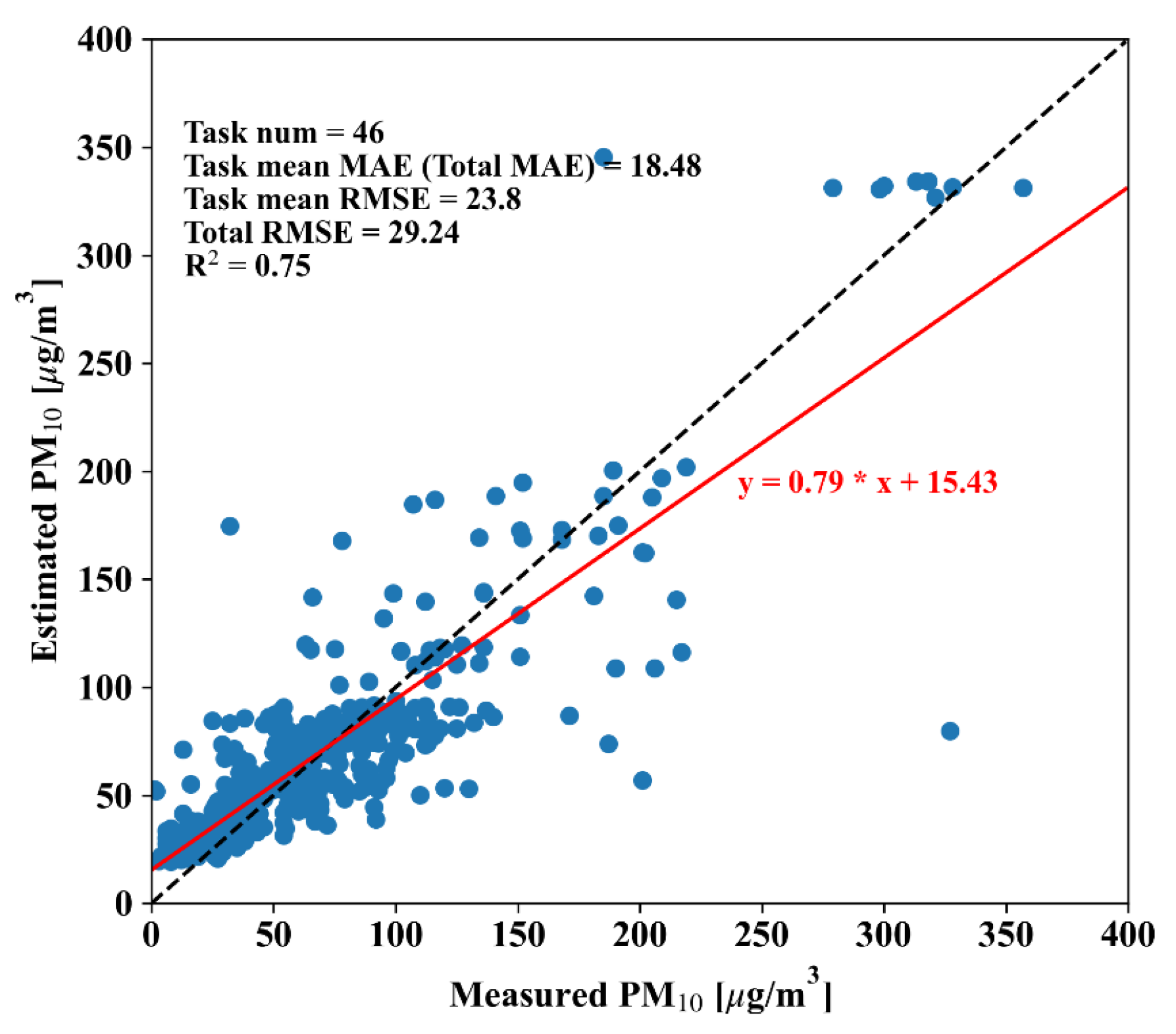
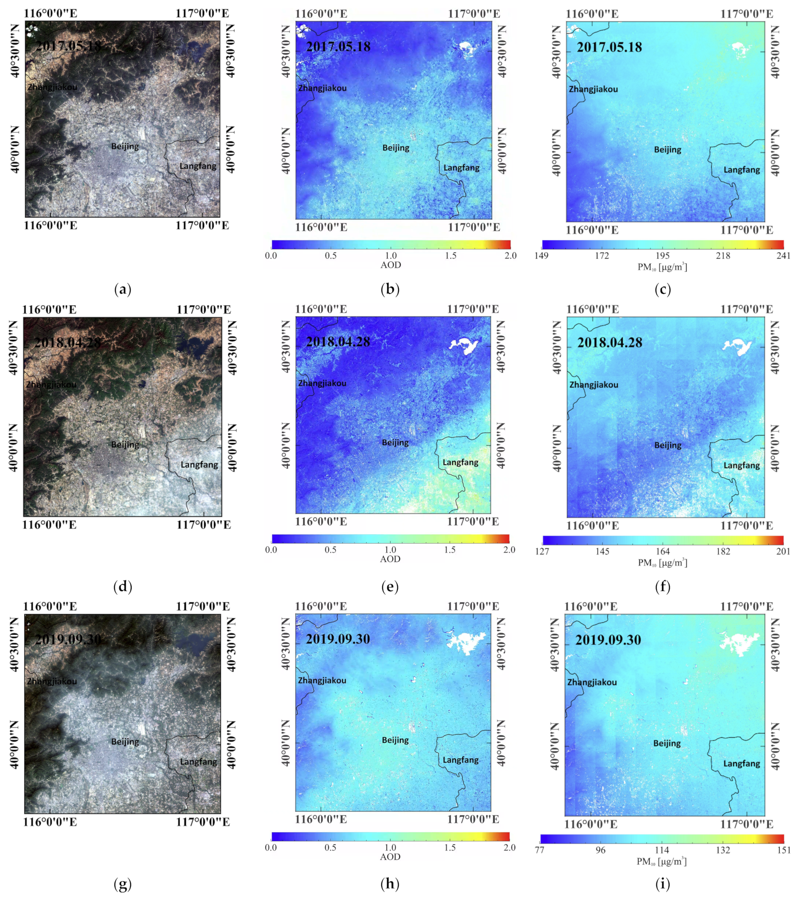
We treat every 4 tasks as a single batch of $N=task\text{\_}num\times (D_s+D_q)=80$ samples. In one epoch, meta-training is conducted on all tasks in a randomly sampled batch. The meta-training process is completed when the number of epochs reach 1000. Subsequently, the best epoch, defined as the model with minimum MSE and highest $R^2$ on the meta-validation set is determined. The evaluation of model performance is executed on the meta-test set using the ANN model from the best epoch. The detailed steps of estimating the PM₁₀ concentration using the meta-test set are given as follows: (1) for each task sampled from the meta-test set, the MAML-ANN model is fine-tuned using 20 gradient updates with a fixed step size of 0.1 on the support dataset; (2) the PM₁₀ concentrations are estimated after forward-passing the corresponding query dataset to the model in (1). Figure 3 shows the schematic diagram of training the ANN model with MAML. The evaluation is carried out by comparing the model-estimated PM₁₀ to the ground truths based on metrics of the coefficient of determination ($R^2$), mean absolute error, and root mean square error (RMSE).

$$MAE=\frac{1}{N}{\displaystyle \sum _i^N\left|y-\widehat{y}\right|}$$

(4)

$$RMSE=\sqrt{\frac{1}{N}{{\displaystyle \sum _i^N\left(y-\widehat{y}\right)}}^2}$$

(5)

where $N$ represents the number of samples; $y$ and $\widehat{y}$ are the measured and model-estimated ground-level PM₁₀ concentrations, respectively. It is noteworthy that in the meta-test phase, the daily mean values of PM₁₀ are not used to ensure the reliability of the verification results.

4. Results

The proposed MAML-ANN method is implemented using the deep learning platform of PyTorch (version 2.2.0). In this study, tasks sampled from the meta-training set are used to train MAML-ANN model to learn the nonlinearity across time from only a small number of data samples and transfer the knowledge learned from coarse spatial resolution to high spatial resolution. At the meta-test stage, a total of 46 available tasks sampled from the meta-test set are used to evaluate the generalization and accuracy of the MAML-ANN model in estimating high-resolution PM₁₀ concentrations based on a small number of data samples (i.e., 10 unseen samples per task). Furthermore, the MAML-ANN model is first fine-tuned on support datasets and then reports the performance metrics on query datasets. In order to validate the estimated PM₁₀ directly against the measured PM₁₀, inverse normalization is performed on the model-estimated PM₁₀. The achieved validation result is shown in Figure 4. The coefficient of determination ($R^2$) indicates that the ANN model trained with MAML can explain 75% of PM₁₀ with 15 variables. In addition, the MAML-ANN model is observed to yield reasonable PM₁₀ estimations in the study area using only 10 training samples, with MAE (task mean MAE), task mean RMSE, and RMSE of 18.48 ${\mu \mathrm{g}/\mathrm{m}}^3$, 23.8 ${\mu \mathrm{g}/\mathrm{m}}^3$, and 29.24 ${\mu \mathrm{g}/\mathrm{m}}^3$, respectively. The slope of estimated PM₁₀ to measured PM₁₀ is less than 1 (i.e., 0.79), with bias score of 15.43 ${\mu \mathrm{g}/\mathrm{m}}^3$, implying that the MAML-ANN model tends to underestimate moderate to high ground-level PM₁₀ concentrations (>73 ${\mu \mathrm{g}/\mathrm{m}}^3$). The estimation performance of the MAML-ANN model at high PM₁₀ concentrations (>100 ${\mu \mathrm{g}/\mathrm{m}}^3$) is somewhat unsatisfactory. This can be attributed to the fact that the number of high pollution days (34.4%) is much lower than that under general conditions (65.6%), leading the model unable to effectively learn the relationships between meteorological conditions and PM₁₀ concentrations under high air pollution circumstance [15]. The uncertainties in ERA5-Land reanalysis dataset and aerosol products, and the coarse spatial resolution of the used ERA5-Land reanalysis dataset also negatively contribute to the accuracy of the estimated PM₁₀ concentrations.

We further break down the PM₁₀ estimation performance of the MAML-ANN model by four station types (i.e., urban, suburban, background, and roadside) using a setting of $D_s=10$, while $D_q=$ all remaining samples during meta-test, as shown in

Table 4. Estimation performance of the MAML-ANN model in Beijing with respect to station types. The number of samples in support dataset is of 10, while the query dataset contains all remaining samples on that day.

Station Type	MAE	RMSE	${\mathit{R}}^2$
Urban	15.47	21.35	0.87
Suburban	22.34	31.95	0.72
Background	30.6	45.32	0.51
Roadside	14.64	21.45	0.89
All	19.44	28.89	0.77

. The MAML-ANN model is found to have the strongest ground-level PM₁₀ estimation capability in roadside stations, with $R^2$ of 0.89, as well as MAE and RMSE values of 14.64 ${\mu \mathrm{g}/\mathrm{m}}^3$ and 21.45 ${\mu \mathrm{g}/\mathrm{m}}^3$, respectively. Coefficient of determination for urban stations is of 0.87, along with MAE and RMSE values are of 15.47 ${\mu \mathrm{g}/\mathrm{m}}^3$ and 21.35${\mu \mathrm{g}/\mathrm{m}}^3$, respectively, revealing good matches of estimated PM₁₀ with measured PM₁₀ in this station type. MAE and RMSE values for suburban stations are of 22.34 ${\mu \mathrm{g}/\mathrm{m}}^3$ and 31.95${\mu \mathrm{g}/\mathrm{m}}^3$, respectively, which are relatively high; however, with an $R^2$ of 0.72, a model-estimated PM₁₀ can be concluded that agrees reasonably with the measured PM₁₀ in this station type. The coefficient of determination for background stations is less than 0.6 ($R^2$ = 0.51), suggesting relatively poor agreement between estimated PM₁₀ and measured PM₁₀ in this station type. According to all three metrics (i.e., MAE, RMSE, and $R^2$) in Table 4, PM₁₀ estimation accuracies of the MAML-ANN model in the four types of stations, from high to low, are as follows: roadside > urban > suburban > background, consistent with Zheng et al. [12]. The intra-station variations in particulate matter of roadside and urban stations are much smaller than those of the suburban and background stations. Therefore, the proposed model can better capture the spatial autocorrelations among roadside and urban stations [53]. The comparison results among different station types also explain the outliers (one extremely underestimated point and one extremely overestimated point) in Figure 4, which are caused by the undesirable estimation performance of the MAML-ANN model in background stations. The total $R^2$ is of 0.77, with the MAE value of 19.44 ${\mu \mathrm{g}/\mathrm{m}}^3$ and RMSE value of 28.89 ${\mu \mathrm{g}/\mathrm{m}}^3$, on average. These results suggest that the ANN model initialized by MAML performs reasonably in the study area and is able to estimate reliable high-resolution PM₁₀ concentrations using only 10 training samples.

Figure 5 exhibits several examples of the estimated high-resolution (60 m × 60 m) PM₁₀ distributions by the MAML-ANN model using only 10 data samples. Gaps in the second and third columns of Figure 5 represent no data due to the lack of available model predictors. Figure 5c shows that Beijing and its surrounding areas were suffering from heavy PM₁₀ pollution on 18 May 2017, with most PM₁₀ concentrations in the study area larger than 150 ${\mu \mathrm{g}/\mathrm{m}}^3$. Evident haze is observed in the lower right area in Figure 5d, which is successfully recognized by the MAML-ANN model and then estimated to be at the corresponding area in Figure 5f. Similarly, Figure 5g also finds obvious haze, reflecting in the corresponding model-estimated PM₁₀ spatial distribution [see Figure 5i]. Because the meteorological conditions used in this study are of coarse spatial resolution (0.1°), the model-estimated 60 m × 60 m PM₁₀ concentration distributions are inevitably impacted by grid-like noise, as shown in the upper left area and left area of Figure 5f,i, respectively. PM₁₀ is shown to have a high linear correlation with AOD [54]. However, the similarity in spatial variability between Sentinel-2 AOD and corresponding MAML-ANN-estimated PM₁₀ is relatively low due to the association of high PM₁₀ levels with a broad scale synoptic system [55]. Overall, those PM₁₀ spatial distributions point out that our MAML-ANN model is able to capture the spatial variation of ground-level PM₁₀ concentrations at a spatial resolution of 60 m × 60 m after seeing only 10 training samples.

To better evaluate the PM₁₀ estimation performance of the proposed MAML-ANN model, we further conduct a case study in Changsha, China. As shown in Figure S2, the correlation of determination is extremely high ($R^2$ = 0.99), as well as MAE (task mean MAE), task mean RMSE, and RMSE of 6.71 ${\mu \mathrm{g}/\mathrm{m}}^3$, 9.08${\mu \mathrm{g}/\mathrm{m}}^3$, and 9.12 ${\mu \mathrm{g}/\mathrm{m}}^3$, respectively, pointing out that the MAML-ANN model is able to obtain reliable PM₁₀ estimations in Changsha using only five training samples. Due to (1) the meteorological conditions used in the study being of coarse spatial resolution (0.1°); (2) the spatial variability in the used Sentinel-2 L2A AOD distributions over Changsha being inferior to those retrieved by the application of Yang et al.’s algorithm; and (3) the employed PM₁₀ stations in Changsha being concentrated in a very small area in the lower right corner of a Sentinel-2 image [see Figure S1], the obtained PM₁₀ distributions [see Figure S3] suffer from severe grid-like noise and cannot well present the spatial variability of PM₁₀ concentration distributions. The obtained PM₁₀ estimations of Changsha suggest that our MAML-ANN model has the potential to provide high-resolution PM₁₀ concentrations for data-sparse, heavily polluted, and small regions.

5. Comparison

5.1. Baseline

Another popular approach for tackling problems with few samples is transfer learning, which usually uses a model that is pre-trained on a large body of data as an initialization for datasets with fewer examples [27]. To better evaluate the generalization of the MAML-ANN model, we compare it with a model pre-trained on all available data in the meta-training set using regular gradient descent. The pre-trained model has the same architecture and loss function as the MAML-ANN model and is likewise trained with Adam with a step size of $\alpha =0.01$ using a batch size of 80 samples. The optimal epoch is determined by the entire meta-validation set (epoch with minimal MAE as well as the highest $R^2$) to be consistent with the proposed model. At test time, the 46 tasks sampled from the meta-test set are utilized to evaluate the model’s adaptability to new unseen tasks based on only a few examples. To make comparison fair, we fine-tune the pre-trained ANN (P-ANN) model with gradient descent on the 10 provided pairs in the support datasets using an automatically tuned step size, and then report the performance metrics on query datasets.

Figure 6a,b illustrate the MAE and RMSE values for an increasing number of gradient updates during fine-tuning, respectively. The zero step case, representing no adaption during fine-tuning, finds that the PM₁₀ estimations of neither the MAML-trained nor the pre-trained ANN model are high in accuracy, with MAE and RMSE values larger than 35 ${\mu \mathrm{g}/\mathrm{m}}^3$ and 55 ${\mu \mathrm{g}/\mathrm{m}}^3$, respectively. The MAE and RMSE values drop sharply until the gradient steps reach two and then decrease slowly with additional gradient updates, indicating that the estimation performance of both two models continue to improve as the gradient steps increase. The metrics of MAE and RMSE also signify that the two ANN models, i.e., learned with MAML and pre-training, are able to estimate the ground-level PM₁₀ concentrations in the study area after being fine-tuned with multiple gradient steps (i.e., 20), with MAE less than 23 ${\mu \mathrm{g}/\mathrm{m}}^3$ as well as RMSE values not higher than 33 ${\mu \mathrm{g}/\mathrm{m}}^3$. Without any fine-tuning, the MAML-ANN model (MAE of 37.27 ${\mu \mathrm{g}/\mathrm{m}}^3$, RMSE of 56.21 ${\mu \mathrm{g}/\mathrm{m}}^3$) only slightly outperforms the P-ANN model (MAE of 42.23 ${\mu \mathrm{g}/\mathrm{m}}^3$, RMSE of 58.51 ${\mu \mathrm{g}/\mathrm{m}}^3$). However, when fine-tuning the parameters slightly (i.e., one gradient update), the MAML-ANN model (MAE of 28.35 ${\mu \mathrm{g}/\mathrm{m}}^3$, RMSE of 39.08 ${\mu \mathrm{g}/\mathrm{m}}^3$) surpass the P-ANN model (MAE of 33.97 ${\mu \mathrm{g}/\mathrm{m}}^3$, RMSE of 47.67 ${\mu \mathrm{g}/\mathrm{m}}^3$) by a large margin, implying the superiority of the MAML-ANN model in fast adaption. Additionally, the estimation errors in the MAML-ANN model are substantially lower than in the baseline fine-tuning approach, indicating that the MAML-ANN model also has merit in PM₁₀ estimation accuracy. These comparison results highlight a distinct difference between the MAML-ANN model and the P-ANN model. The relationship among aerosol, meteorological conditions, and PM₁₀ concentrations varies daily [9]. Pre-training on all of the tasks entails training a network to regress to random predictor–predictant functions; whereas MAML learns to model the broadly transferrable spatiotemporal interlinkage among aerosol, meteorological conditions, and PM₁₀ concentration. Consequently, the MAML-ANN model is easier and faster to fine-tune than the P-ANN model. In comparison with the model initialized with pre-training, our model initialized with MAML is more amenable to fast adaptation and has higher accuracy for ground-level PM₁₀ estimation based on small datasets.

5.2. Competitors

To the best of our knowledge, no studies have used MAML to train an artificial neural network to estimate the spatial distribution of PM₁₀. Therefore, the 30 m × 30 m PM₁₀ concentrations estimated from a multispectral empirical model (MEM) are selected here for comparison purpose [54]. Limited by the coarse spatial resolution of available satellite aerosol data, few satellite-retrieved PM₁₀ are at high spatial resolution. To this end, several recent state-of-the-art works showing outstanding performance on coarse resolution PM₁₀ estimation are also considered as competitors for comparison with the proposed method [56,57]. The three competitors are briefly reviewed in the following.

GRU-LSTM-FC: A deep neural network consisting of fully connected (FC), LSTM, and gated recurrent units (GRU) is proposed in this work to estimate the spatial distribution of PM_2.5 and PM₁₀ at 250 m × 250 m resolution. The proposed framework accepts the original calibrated radiance of MODIS-Level 1 images as input, thereby avoiding the intermediate computations for atmospheric reflectance or AOD calculation.

MEM: The relationship between atmospheric reflectance and AOD is established using Landsat 8 Operational Land Imager (OLI) satellite data. Hereinafter, a MEM regressing from the atmospheric reflectance to PM₁₀ concentration is developed on the basis of the linear relationship between PM₁₀ and AOD.

RF: A random forest (RF) approach is utilized to estimate spatially continuous AOD and subsequent PM₁₀ and PM_2.5 concentrations combining multiple satellite-based data with model-based data and auxiliary data.

Comparisons of the proposed MAML-ANN model with the three competitors (i.e., GRU-LSTM-FC, MEM, and RF) for spatial estimation of PM₁₀ are shown in

Table 5. Comparisons of the proposed MAML-ANN model with other methods for spatial estimation of PM₁₀.

Method	Study Area	Time Period	RMSE ($\mu \mathbf{g}/{\mathbf{m}}^3$)	Resolution of PM10	Ref.
GRU-LSTM-FC	Tehran (Iran)	2019–2020	23.79	250 m × 250 m	[57]
MEM	Delhi (India)	2016	18.99	30 m × 30 m	[54]
RF	East Asia	2016	26.9	6 km × 6 km	[56]
MAML-ANN	Beijing	2013–2019	28.89	60 m × 60 m	This study

. Compared with the two coarse resolution competitors (i.e., GRU-LSTM-FC and RF), the RMSE value of the MAML-ANN model is increased by 5.1 ${\mu \mathrm{g}/\mathrm{m}}^3$ and 1.99 ${\mu \mathrm{g}/\mathrm{m}}^3$, respectively; however, the spatial resolution of model-estimated PM₁₀ is significantly improved by 4.17 and 100 times, respectively. It is worth noting that both the GRU-LSTM-FC model and RF model are developed on the basis of a large number of data, thereby being difficult to apply to data-sparse regions. The spatial resolution and RMSE value of the MEM estimated PM₁₀ are both superior to that of the MAML-ANN estimated PM₁₀. However, we notice that the MEM only reports the estimation performance on an extremely small number of samples (i.e., 11 samples), whereas the MAML-ANN model tests on more than 460 samples. Because MEM is site-specific [54], we further compare the MAML-ANN estimated PM₁₀ in roadside stations with all MEM estimated PM₁₀. The RMSE value for the MAML-ANN estimated PM₁₀ is slightly higher than that of the MEM estimated PM₁₀ (21.45 ${\mu \mathrm{g}/\mathrm{m}}^3$ vs. 18.99 ${\mu \mathrm{g}/\mathrm{m}}^3$); however, the superior $R^2$ (0.88 vs. 0.80) and regression line ($y=0.75x+10.76$ vs. $y=0.74x+65.41$) suggests that the MAML-ANN model outperforms the MEM for high-resolution PM₁₀ estimations. More importantly, benefiting from the usage of MAML, the proposed MAML-ANN model is able to solve one-shot problems (i.e., where only one sample is available), whereas the MEM requires at least three samples to build the empirical model. Overall, the comparison results imply that the proposed method is a low-cost and efficient approach for generation high-resolution PM₁₀ maps in data-sparse regions.

6. Conclusions

Monitoring air pollution in small and local regions can greatly benefit policymakers in formulating PM₁₀ control measures yet is very challenging because of the sparsity of air quality monitoring stations. At present, few studies have mapped PM at high spatial resolution. This study introduces a MAML-trained ANN (MAML-ANN) model for advancing the estimation of ground-level PM₁₀ concentrations at high spatial resolution by integrating 60 m × 60 m Sentinel-2 AOD (10 km × 10 km MOD04_L2 AOD for meta-training and meta-validation set) with 0.1° meteorological conditions (wind speed, wind direction, temperature, and pressure) and other import PM₁₀ predictors (longitude, latitude, DOM, MOY, season, and year). The task is designed to support the model learning the time-varying relationships among aerosols, meteorological conditions, and PM₁₀. We conducted the experiment on 32 air quality monitoring stations in Beijing over a period of ~7 years from 2013 to 2019. The ANN model is trained on a large number of historic tasks (from 2013 to 2016) with coarse spatial resolution, and model performance and generalization is then evaluated on holdout high-resolution tasks (from 2017 to 2019) and a case study in Changsha.

The results of the validation show that our MAML-ANN model is able to estimate ground-level PM₁₀ concentrations over the study area at a spatial resolution of 60 m × 60 m with coefficient of determination of 0.75, as well as MAE and RMSE values of 18.48 ${\mu \mathrm{g}/\mathrm{m}}^3$ and 29.24 ${\mu \mathrm{g}/\mathrm{m}}^3$, respectively. The MAML-ANN model makes PM₁₀ estimations relatively better under general conditions; however, its performance in estimating high PM₁₀ concentrations is unsatisfactory due to the insufficient training data on high-pollution situations. Station type also shows a non-negligible impact on the PM₁₀ estimation accuracy of the proposed model. The recommended annual PM₁₀ concentrations of World Health Organization (WHO) air quality guidelines (AQGs) is of 15 ${\mu \mathrm{g}/\mathrm{m}}^3$, which is quite similar to the bias score (15.43 ${\mu \mathrm{g}/\mathrm{m}}^3$) of the estimated PM₁₀. To this end, the proposed MAML-ANN model is recommended to apply to heavily polluted and small areas.

Validation results in Changsha indicate that the proposed method is able to provide high-quality PM₁₀ estimations; however, much work remains to be done in capturing the spatial variability of high-resolution PM₁₀ estimates.

In comparison with the baseline that is pre-trained with regular gradient descent, MAE value of our MAML-ANN model is apparently more acceptable (18.48 ${\mu \mathrm{g}/\mathrm{m}}^3$ vs. 22.3 ${\mu \mathrm{g}/\mathrm{m}}^3$) along with the lower RMSE value (29.24 ${\mu \mathrm{g}/\mathrm{m}}^3$ vs. 32.56 ${\mu \mathrm{g}/\mathrm{m}}^3$). In addition, our model trained with MAML is also superior in fast adaption with MAE and RMSE values dropping much more quickly than those of the P-ANN model when slightly fine-tuning the parameters. The comparison results demonstrate that the incorporation of MAML can greatly improve the estimation accuracy and is beneficial for quick adaption, providing a powerful tool for estimating ground-level PM₁₀ concentrations at high spatial resolution with scarce satellite-derived AOD products. In conclusion, the model outcomes show that our MAML-ANN model is capable of providing 60 m × 60 m ground-level PM₁₀ distributions in detail with only 10 samples.

Compared with several recent state-of-the-art methods estimating PM₁₀ at coarse resolution, the proposed method greatly improves the spatial resolution of estimated PM₁₀ with slightly inferior estimation accuracy. In comparison with the competitor mapping PM₁₀ at high resolution, the proposed method has merits in estimation accuracy.

The main contributions of the proposed method are as follows:

(1)

A MAML-trained ANN model is proposed to estimate the ground-level PM₁₀ at high resolution (60 m × 60 m) over the study area.

(2)

The proposed MAML-ANN model is able to estimate PM₁₀ in the study area and has the potential to obtain high-resolution PM₁₀ over other data-sparse and small regions with heavy pollution.

(3)

MAML-ANN improves the PM₁₀ estimation performance compared with the pre-trained ANN.

Ambient meteorology plays a substantial role in inferring the ground-level PM₁₀ concentrations; however, its drawback of potentially introducing grid-like noise into the estimated PM₁₀ distributions due to the coarse spatial resolution (0.1°) should be further taken into account. Additionally, much work remains to be carried out to address the underestimation of ground-level PM₁₀ concentrations by the model. To improve the performance of the proposed model, future research should include more PM₁₀ drivers at fine resolution as model inputs. Furthermore, improving the model architecture also contributes to the accuracy of the PM₁₀ estimates. In future work, field studies need to be undertaken to better verify the method.

References

1. Lim, S.S.; Vos, T.; Flaxman, A.D.; Danaei, G.; Shibuya, K.; Adair-Rohani, H.; AlMazroa, M.A.; Amann, M.; Anderson, H.R.; Andrews, K.G. A comparative risk assessment of burden of disease and injury attributable to 67 risk factors and risk factor clusters in 21 regions, 1990–2010: A systematic analysis for the Global Burden of Disease Study 2010. Lancet 2012, 380, 2224–2260. [Google Scholar] [CrossRef] [PubMed]
2. Pope, C.A., III; Burnett, R.T.; Thun, M.J.; Calle, E.E.; Krewski, D.; Ito, K.; Thurston, G.D. Lung cancer, cardiopulmonary mortality, and long-term exposure to fine particulate air pollution. JAMA 2002, 287, 1132–1141. [Google Scholar] [CrossRef] [PubMed]
3. Lelieveld, J.; Klingmüller, K.; Pozzer, A.; Pöschl, U.; Fnais, M.; Daiber, A.; Münzel, T. Cardiovascular disease burden from ambient air pollution in Europe reassessed using novel hazard ratio functions. Eur. Heart J. 2019, 40, 1590–1596. [Google Scholar] [CrossRef] [PubMed]
4. Lelieveld, J.; Evans, J.S.; Fnais, M.; Giannadaki, D.; Pozzer, A. The contribution of outdoor air pollution sources to premature mortality on a global scale. Nature 2015, 525, 367–371. [Google Scholar] [CrossRef] [PubMed]
5. Stirnberg, R.; Cermak, J.; Andersen, H. An analysis of factors influencing the relationship between satellite-derived AOD and ground-level PM10. Remote Sens. 2018, 10, 1353. [Google Scholar] [CrossRef]
6. Stirnberg, R.; Cermak, J.; Fuchs, J.; Andersen, H. Mapping and understanding patterns of air quality using satellite data and machine learning. J. Geophys. Res. Atmos. 2020, 125, e2019JD031380. [Google Scholar] [CrossRef]
7. Al-Saadi, J.; Szykman, J.; Pierce, R.B.; Kittaka, C.; Neil, D.; Chu, D.A.; Remer, L.; Gumley, L.; Prins, E.; Weinstock, L.; et al. Improving National Air Quality Forecasts with Satellite Aerosol Observations. Bull. Am. Meteorol. Soc. 2005, 86, 1249–1262. [Google Scholar] [CrossRef]
8. Yang, Y.; Cermak, J.; Yang, K.; Pauli, E.; Chen, Y. Land Use and Land Cover Influence on Sentinel-2 Aerosol Optical Depth below City Scales over Beijing. Remote Sens. 2022, 14, 4677. [Google Scholar] [CrossRef]
9. Lee, H.J.; Liu, Y.; Coull, B.; Schwartz, J.D.; Koutrakis, P. A novel calibration approach of MODIS AOD data to predict PM2.5 concentrations. Atmos. Chem. Phys. 2011, 11, 7991–8002. [Google Scholar] [CrossRef]
10. Gupta, P.; Christopher, S.A. Particulate matter air quality assessment using integrated surface, satellite, and meteorological products: Multiple regression approach. J. Geophys. Res. Atmos. 2009, 114, D14205. [Google Scholar] [CrossRef]
11. You, W.; Zang, Z.; Zhang, L.; Li, Z.; Chen, D.; Zhang, G. Estimating ground-level PM10 concentration in northwestern China using geographically weighted regression based on satellite AOD combined with CALIPSO and MODIS fire count. Remote Sens. Environ. 2015, 168, 276–285. [Google Scholar] [CrossRef]
12. Zheng, T.; Bergin, M.H.; Hu, S.; Miller, J.; Carlson, D.E. Estimating ground-level PM2.5 using micro-satellite images by a convolutional neural network and random forest approach. Atmos. Environ. 2020, 230, 117451. [Google Scholar] [CrossRef]
13. Hu, X.; Waller, L.A.; Al-Hamdan, M.Z.; Crosson, W.L.; Estes, M.G., Jr.; Estes, S.M.; Quattrochi, D.A.; Sarnat, J.A.; Liu, Y. Estimating ground-level PM2. 5 concentrations in the southeastern US using geographically weighted regression. Environ. Res. 2013, 121, 1–10. [Google Scholar] [CrossRef]
14. Koelemeijer, R.; Homan, C.; Matthijsen, J. Comparison of spatial and temporal variations of aerosol optical thickness and particulate matter over Europe. Atmos. Environ. 2006, 40, 5304–5315. [Google Scholar] [CrossRef]
15. Ma, W.; Yuan, Z.; Lau, A.K.; Wang, L.; Liao, C.; Zhang, Y. Optimized neural network for daily-scale ozone prediction based on transfer learning. Sci. Total Environ. 2022, 827, 154279. [Google Scholar] [CrossRef]
16. Taheri Shahraiyni, H.; Sodoudi, S.J.A. Statistical modeling approaches for PM10 prediction in urban areas; A review of 21st-century studies. Atmosphere 2016, 7, 15. [Google Scholar] [CrossRef]
17. Cermak, J.; Knutti, R. Beijing Olympics as an aerosol field experiment. Geophys. Res. Lett. 2009, 36, L10806. [Google Scholar] [CrossRef]
18. Perez, P. Combined model for PM10 forecasting in a large city. Atmos. Environ. 2012, 60, 271–276. [Google Scholar] [CrossRef]
19. Park, S.; Kim, M.; Kim, M.; Namgung, H.-G.; Kim, K.-T.; Cho, K.H.; Kwon, S.-B. Predicting PM10 concentration in Seoul metropolitan subway stations using artificial neural network (ANN). J. Hazard. Mater. 2018, 341, 75–82. [Google Scholar] [CrossRef]
20. Wei, J.; Huang, B.; Sun, L.; Zhang, Z.; Wang, L.; Bilal, M. A simple and universal aerosol retrieval algorithm for Landsat series images over complex surfaces. J. Geophys. Res. Atmos. 2017, 122, 13338–13355. [Google Scholar] [CrossRef]
21. Sun, L.; Wei, J.; Bilal, M.; Tian, X.; Jia, C.; Guo, Y.; Mi, X. Aerosol optical depth retrieval over bright areas using Landsat 8 OLI images. Remote Sens. 2016, 8, 23. [Google Scholar] [CrossRef]
22. Yang, Y.; Chen, Y.; Yang, K.; Cermak, J.; Chen, Y. High-resolution aerosol retrieval over urban areas using sentinel-2 data. Atmos. Res. 2021, 264, 105829. [Google Scholar] [CrossRef]
23. Cheng, S.; Shen, H.; Shan, G.; Niu, B.; Bai, W. Visual analysis of meteorological satellite data via model-agnostic meta-learning. J. Vis. 2021, 24, 301–315. [Google Scholar] [CrossRef]
24. Wang, Y.; Yao, Q.; Kwok, J.T.; Ni, L.M. Generalizing from a few examples: A survey on few-shot learning. ACM Comput. Surv. 2020, 53, 1–34. [Google Scholar] [CrossRef]
25. Tseng, G.; Kerner, H.; Nakalembe, C.; Becker-Reshef, I. Learning to predict crop type from heterogeneous sparse labels using meta-learning. In Proceedings of the IEEE/CVF Conference on Computer Vision and Pattern Recognition (CVPR) Workshops, Nashville, TN, USA, 19–25 June 2021; pp. 1111–1120. [Google Scholar]
26. Finn, C.; Abbeel, P.; Levine, S. Model-agnostic meta-learning for fast adaptation of deep networks. In Proceedings of the International Conference on Machine Learning, Sydney, Australia, 6–11 August 2017; pp. 1126–1135. [Google Scholar]
27. Rußwurm, M.; Wang, S.; Korner, M.; Lobell, D. Meta-learning for few-shot land cover classification. In Proceedings of the IEEE/CVF Conference on Computer Vision and Pattern Recognition (CVPR) Workshops, Seattle, WA, USA, 14–19 June 2020; pp. 200–201. [Google Scholar]
28. Janssen, N.A.H.; Fischer, P.; Marra, M.; Ameling, C.; Cassee, F.R. Short-term effects of PM2.5, PM10 and PM2.5–10 on daily mortality in the Netherlands. Sci. Total Environ. 2013, 463–464, 20–26. [Google Scholar] [CrossRef]
29. Tao, Z.; Kokas, A.; Zhang, R.; Cohan, D.S.; Wallach, D. Inferring atmospheric particulate matter concentrations from Chinese social media data. PLoS ONE 2016, 11, e0161389. [Google Scholar] [CrossRef]
30. Zhang, A.; Qi, Q.; Jiang, L.; Zhou, F.; Wang, J. Population exposure to PM2.5 in the urban area of Beijing. PLoS ONE 2013, 8, e63486. [Google Scholar] [CrossRef]
31. Emili, E.; Popp, C.; Wunderle, S.; Zebisch, M.; Petitta, M. Mapping particulate matter in alpine regions with satellite and ground-based measurements: An exploratory study for data assimilation. Atmos. Environ. 2011, 45, 4344–4353. [Google Scholar] [CrossRef]
32. Yang, Y.; Yang, K.; Chen, Y. Aerosol Retrieval Algorithm for Sentinel-2 Images Over Complex Urban Areas. IEEE Trans. Geosci. Remote Sens. 2022, 60, 1–9. [Google Scholar] [CrossRef]
33. Munchak, L.; Levy, R.; Mattoo, S.; Remer, L.; Holben, B.; Schafer, J.; Hostetler, C.; Ferrare, R. MODIS 3 km aerosol product: Applications over land in an urban/suburban region. Atmos. Meas. Tech. 2013, 6, 1747–1759. [Google Scholar] [CrossRef]
34. Yan, X.; Li, Z.; Luo, N.; Shi, W.; Zhao, W.; Yang, X.; Jin, J. A minimum albedo aerosol retrieval method for the new-generation geostationary meteorological satellite Himawari-8. Atmos. Res. 2018, 207, 14–27. [Google Scholar] [CrossRef]
35. Wei, J.; Li, Z.; Peng, Y.; Sun, L. MODIS Collection 6.1 aerosol optical depth products over land and ocean: Validation and comparison. Atmos. Environ. 2019, 201, 428–440. [Google Scholar] [CrossRef]
36. Wen, C.; Liu, S.; Yao, X.; Peng, L.; Li, X.; Hu, Y.; Chi, T. A novel spatiotemporal convolutional long short-term neural network for air pollution prediction. Sci. Total Environ. 2019, 654, 1091–1099. [Google Scholar] [CrossRef]
37. Muñoz Sabater, J. ERA5-Land hourly data from 1950 to 1980. Volume 10. 2021. Available online: https://cds.climate.copernicus.eu/cdsapp#!/dataset/10.24381/cds.e2161bac?tab=overview (accessed on 4 July 2024).
38. Li, Z.; Guo, J.; Ding, A.; Liao, H.; Liu, J.; Sun, Y.; Wang, T.; Xue, H.; Zhang, H.; Zhu, B. Aerosol and boundary-layer interactions and impact on air quality. Natl. Sci. Rev. 2017, 4, 810–833. [Google Scholar] [CrossRef]
39. Li, Y.; Chen, Q.; Zhao, H.; Wang, L.; Tao, R. Variations in PM10, PM2. 5 and PM1. 0 in an urban area of the Sichuan Basin and their relation to meteorological factors. Atmosphere 2015, 6, 150–163. [Google Scholar] [CrossRef]
40. Andersen, H.; Cermak, J.; Stirnberg, R.; Fuchs, J.; Kim, M.; Pauli, E. Assessment of COVID-19 effects on satellite-observed aerosol loading over China with machine learning. Tellus B Chem. Phys. Meteorol. 2021, 73, 1971925. [Google Scholar] [CrossRef]
41. Wang, X.; Dickinson, R.E.; Su, L.; Zhou, C.; Wang, K. PM2.5 pollution in China and how it has been exacerbated by terrain and meteorological conditions. Bull. Am. Meteorol. Soc. 2018, 99, 105–119. [Google Scholar] [CrossRef]
42. Leung, D.M.; Tai, A.P.; Mickley, L.J.; Moch, J.M.; Van Donkelaar, A.; Shen, L.; Martin, R.V. Synoptic meteorological modes of variability for fine particulate matter (PM2.5) air quality in major metropolitan regions of China. Atmos. Chem. Phys. 2018, 18, 6733–6748. [Google Scholar] [CrossRef]
43. Grange, S.K.; Carslaw, D.C.; Lewis, A.C.; Boleti, E.; Hueglin, C. Random forest meteorological normalisation models for Swiss PM 10 trend analysis. Atmos. Chem. Phys. 2018, 18, 6223–6239. [Google Scholar] [CrossRef]
44. Zhang, K.; Zhang, X.; Song, H.; Pan, H.; Wang, B. Air Quality Prediction Model Based on Spatiotemporal Data Analysis and Metalearning. Wirel. Commun. Mobile Comput. 2021, 2021, 9627776. [Google Scholar] [CrossRef]
45. Fong, I.H.; Li, T.; Fong, S.; Wong, R.K.; Tallon-Ballesteros, A.J. Predicting concentration levels of air pollutants by transfer learning and recurrent neural network. Knowl.-Based Syst. 2020, 192, 105622. [Google Scholar] [CrossRef]
46. Ma, J.; Cheng, J.C.; Lin, C.; Tan, Y.; Zhang, J. Improving air quality prediction accuracy at larger temporal resolutions using deep learning and transfer learning techniques. Atmos. Environ. 2019, 214, 116885. [Google Scholar] [CrossRef]
47. Chellali, M.; Abderrahim, H.; Hamou, A.; Nebatti, A.; Janovec, J. Artificial neural network models for prediction of daily fine particulate matter concentrations in Algiers. Environ. Sci. Pollut. Res. 2016, 23, 14008–14017. [Google Scholar] [CrossRef] [PubMed]
48. Grivas, G.; Chaloulakou, A. Artificial neural network models for prediction of PM10 hourly concentrations, in the Greater Area of Athens, Greece. Atmos. Environ. 2006, 40, 1216–1229. [Google Scholar] [CrossRef]
49. Papanastasiou, D.; Melas, D.; Kioutsioukis, I. Development and assessment of neural network and multiple regression models in order to predict PM10 levels in a medium-sized Mediterranean city. Water Air Soil Pollut. 2007, 182, 325–334. [Google Scholar] [CrossRef]
50. Pérez, P.; Trier, A.; Reyes, J. Prediction of PM2.5 concentrations several hours in advance using neural networks in Santiago, Chile. Atmos. Environ. 2000, 34, 1189–1196. [Google Scholar] [CrossRef]
51. He, K.; Zhang, X.; Ren, S.; Sun, J. Delving deep into rectifiers: Surpassing human-level performance on imagenet classification. In Proceedings of the IEEE International Conference on Computer Vision (ICCV), Santiago, Chile, 7–13 December 2015; pp. 1026–1034. [Google Scholar]
52. Kingma, D.P.; Ba, J. Adam: A method for stochastic optimization. In Proceedings of the International Conference on Learning Representations (ICLR), San Diego, CA, USA, 7–9 May 2015. [Google Scholar]
53. Zheng, T.; Bergin, M.H.; Sutaria, R.; Tripathi, S.N.; Caldow, R.; Carlson, D.E. Gaussian process regression model for dynamically calibrating and surveilling a wireless low-cost particulate matter sensor network in Delhi. Atmos. Meas. Tech. 2019, 12, 5161–5181. [Google Scholar] [CrossRef]
54. Saraswat, I.; Mishra, R.K.; Kumar, A. Estimation of PM10 concentration from Landsat 8 OLI satellite imagery over Delhi, India. Remote Sens. Appl. Soc. Environ. 2017, 8, 251–257. [Google Scholar] [CrossRef]
55. Miao, Y.; Guo, J.; Liu, S.; Liu, H.; Li, Z.; Zhang, W.; Zhai, P. Classification of summertime synoptic patterns in Beijing and their associations with boundary layer structure affecting aerosol pollution. Atmos. Chem. Phys. 2017, 17, 3097–3110. [Google Scholar] [CrossRef]
56. Park, S.; Shin, M.; Im, J.; Song, C.-K.; Choi, M.; Kim, J.; Lee, S.; Park, R.; Kim, J.; Lee, D.-W.; et al. Estimation of ground-level particulate matter concentrations through the synergistic use of satellite observations and process-based models over South Korea. Atmos. Chem. Phys. 2019, 19, 1097–1113. [Google Scholar] [CrossRef]
57. Imani, M. Particulate matter (PM2.5 and PM10) generation map using MODIS Level-1 satellite images and deep neural network. J. Environ. Manag. 2021, 281, 111888. [Google Scholar] [CrossRef] [PubMed]
Figure 1. Locations of the 35 air quality monitoring stations in Beijing, including 12 urban stations (red dots, numbered 1–12), 11 suburban stations (blue squares, numbered 13–23), 7 background stations (yellow stars, numbered 24–30), and 5 roadside stations (green triangles, numbered 31–35). The zoom-out view of the black dashed box is shown in the right part of the figure.
Remotesensing 16 02498 g001
Figure 2. An example of a sampling a task. All samples in a task are drawn on the same day but from different stations. Red triangles, black dots, and green stars represent the stations that are selected to form the support dataset, query dataset, and unselected, respectively.
Remotesensing 16 02498 g002
Figure 3. Schematic diagram of training the ANN model with MAML.
Remotesensing 16 02498 g003
Figure 4. Scatter plot displaying the MAML-ANN model estimations for ground-level PM10 concentrations using a D s = D q = 10 setting. Also shown are the coefficient of determination ( R 2 ), slope (red solid line), 1:1 line (black dotted line), task mean MAE (total MAE), task mean RMSE, and total RMSE. The relatively high R 2 shows that the model covers the majority of occurring variance. However, an underestimation of higher PM10 concentrations leads to a lower slope.
Remotesensing 16 02498 g004
Figure 5. Sentinel-2 true color images, Sentinel-2 AOD, and corresponding model-estimated PM10 concentrations spatial distributions at a spatial resolution of 60 m × 60 m. White represents no data. (a,d,g) True color Sentinel-2 images for the study area. (b,e,h) Corresponding AOD images from Yang et al.’s study [32]. (c,f,i) Corresponding PM10 concentrations images.
Remotesensing 16 02498 g005
Figure 6. Metrics of (a) MAE and (b) RMSE at meta test time. Note that MAML continues to improve with additional gradient steps without overfitting to the extremely small dataset during meta-testing, achieving estimation errors that are substantially lower than in the baseline fine-tuning approach.
Remotesensing 16 02498 g006