Article

An Inverse Modeling Approach for Retrieving High-Resolution Surface Fluxes of Greenhouse Gases from Measurements of Their Concentrations in the Atmospheric Boundary Layer

by
Iuliia Mukhartova
1,2,3,
Andrey Sogachev
4,
Ravil Gibadullin
2,3,
Vladislava Pridacha
5,
Ibragim A. Kerimov
3 and
Alexander Olchev
2,3,6,*
1
Department of Mathematics, Faculty of Physics, Lomonosov Moscow State University, GSP-1, Leninskie Gory, Moscow 119991, Russia
2
Department of Meteorology and Climatology, Faculty of Geography, Lomonosov Moscow State University, GSP-1, Leninskie Gory, Moscow 119991, Russia
3
Department of Ecology and Environmental Management, Grozny State Oil Technical University, 100, Isaeva Av., Grozny 364024, Russia
4
A.N. Severtsov Institute of Ecology and Evolution, Russian Academy of Science, 33, Leninsky Prospekt, Moscow 119071, Russia
5
Forest Research Institute, Karelian Research Centre of the Russian Academy of Sciences, Petrozavodsk 185910, Russia
6
Laboratory of the Ecosystem-Atmosphere Interactions of the Mire-Forest Landscapes, Yugra State University, 16, Chekhova Str., Khanty-Mansiysk 628000, Russia
*
Author to whom correspondence should be addressed.
Remote Sens. 2024, 16(13), 2502; https://doi.org/10.3390/rs16132502
Submission received: 11 May 2024 / Revised: 1 July 2024 / Accepted: 5 July 2024 / Published: 8 July 2024
(This article belongs to the Special Issue Remote Sensing of the Terrestrial Carbon Cycle)

Abstract

:
This study explores the potential of using Unmanned Aircraft Vehicles (UAVs) as a measurement platform for estimating greenhouse gas (GHG) fluxes over complex terrain. We proposed and tested an inverse modeling approach for retrieving GHG fluxes based on two-level measurements of GHG concentrations and airflow properties over complex terrain with high spatial resolution. Our approach is based on a three-dimensional hydrodynamic model capable of determining the airflow parameters that affect the spatial distribution of GHG concentrations within the atmospheric boundary layer. The model is primarily designed to solve the forward problem of calculating the steady-state distribution of GHG concentrations and fluxes at different levels over an inhomogeneous land surface within the model domain. The inverse problem deals with determining the unknown surface GHG fluxes by minimizing the difference between measured and modeled GHG concentrations at two selected levels above the land surface. Several numerical experiments were conducted using surrogate data that mimicked UAV observations of varying accuracies and density of GHG concentration measurements to test the robustness of the approach. Our primary modeling target was a 6 km2 forested area in the foothills of the Greater Caucasus Mountains in Russia, characterized by complex topography and mosaic vegetation. The numerical experiments show that the proposed inverse modeling approach can effectively solve the inverse problem, with the resulting flux distribution having the same spatial pattern as the required flux. However, the approach tends to overestimate the mean value of the required flux over the domain, with the maximum errors in flux estimation associated with areas of maximum steepness in the surface topography. The accuracy of flux estimates improves as the number of points and the accuracy of the concentration measurements increase. Therefore, the density of UAV measurements should be adjusted according to the complexity of the terrain to improve the accuracy of the modeling results.

1. Introduction

Accurate and comprehensive data on greenhouse gas (GHG) emissions and uptakes by terrestrial ecosystems are critical as they regulate GHG concentrations in the atmosphere. Experts from the Intergovernmental Panel on Climate Change (IPCC) attribute modern climate change to increasing GHGs from natural and anthropogenic sources [1,2,3]. At the ecosystem scale, sources and sinks of GHGs, such as carbon dioxide (CO2) and methane (CH4), are commonly quantified using the eddy covariance (EC) measurement technique [4,5,6,7]. Locally derived data from this method help to validate various algorithms for estimating the net ecosystem exchange (NEE) of CO2 and fluxes of other GHGs at regional and global scales using satellite [8,9] and aircraft [10,11] remote sensing measurements. However, the lack of in situ measurements makes it difficult to accurately describe the natural diversity of plant community responses to changing environmental conditions.
Despite the widespread network of monitoring stations worldwide, such as FLUXNET [12], there are still many areas and biomes around the globe where information on GHG fluxes between the Earth’s surface and the atmosphere is incomplete or non-existent [13,14,15]. Standard flux measurement techniques, such as the eddy covariance method, face methodological limitations in some locations due to significant variability in land surface topography, land use, and vegetation mosaic [4,16]. Instead, other methods of estimating NEE based on different principles may also be used. These include chamber methods [17,18,19] and biometric approaches such as plant growth assessment and stock inventories [20]. These methods are able to representatively quantify the CO2 and other GHG exchanges at smaller spatial scales than EC measurements [4]. However, some method limitations [4,17] and heterogeneity in the ecosystem under study, such as variations in soil properties (e.g., structure, carbon, and nitrogen content), soil environmental conditions (e.g., soil temperature and moisture), or plant community composition, may lead to large biases in regional flux estimates [21].
Unmanned Aircraft Vehicles (UAVs) equipped with appropriate sensors are a good alternative to traditional methods for various environmental observations [22]. UAVs have been used primarily for analysis of surface and vegetation structure [23,24] and meteorological observations [25,26,27], but they are now being employed to measure GHG concentrations [28] and GHG emissions and uptakes [29,30,31]. It has been shown that multi-platform systems or drone swarms carrying a mobile sensor network help estimate emissions from GHG point sources [32,33]. UAVs equipped with multi- or hyperspectral and GHG concentration measurement instruments can be used to study the spatial variability of fluxes in small areas where direct GHG flux measurements are difficult or impossible [11]. However, there have been only a few attempts to obtain flux information from UAV concentration measurements [34,35]. While drone-based flux measurements’ potential as a relatively low-cost and mobile complement to EC is promising, many questions remain regarding the uncertainties in the resulting flux estimates, the optimal flight strategy, the required turbulent transport model, and the data-model fusion algorithms [35].
The main objective of this proof-of-concept study is to explore the possibility of estimating GHG fluxes over complex areas using UAVs as a measurement platform for GHG concentrations. We propose and test a novel approach for estimating CO2 and CH4 fluxes using CO2 and CH4 concentration data collected at two levels above the surface. Our approach involves using a three-dimensional hydrodynamic model to determine the airflow parameters that impact the distribution of GHG concentrations. The model is primarily aimed at solving the forward problem, namely, calculating the stationary distribution of the GHG concentration over a non-uniform surface, given the GHG fluxes at the lower boundary of the computational domain. The inverse problem of determining the unknown GHG flux involves minimizing the difference between measured and modeled GHG concentrations at two levels above the ground surface. In this study, the measured CO2 and CH4 concentrations were taken from the modeled data and used as a surrogate for the drone measurements to test the concept.
A forested area in the foothills of the Greater Caucasus Mountains in Russia, characterized by highly complex topography and mosaic vegetation, was selected as the primary target area for the study. This area is the subject of intensive studies of GHG fluxes using ground-based and remote sensing methods implemented within the Russian Pilot Project on Carbon Measurement Supersites [36].

2. Materials and Methods

2.1. Forward Modeling

2.1.1. Airflow Modeling

To simulate GHG transport in the atmospheric boundary layer (ABL), we applied the three-dimensional RANS (Reynolds-averaged Navier–Stokes) model developed by Mukhartova et al. [37,38,39]. The model is based on the solution of the vector Navier–Stokes and continuity equation system and adopts the 1.5-closure scheme. This scheme is built on the Boussinesq hypothesis and calculates the turbulent diffusion coefficients (KT) using the turbulent kinetic energy (E) and the dissipation rate of E (ε). The scheme balances computational complexity, model accuracy, and availability of experimental data used for model validation [37,39,40].
The model allows estimation of the airflow parameters between the land surface with given orography h x , y covered by vegetation canopy and the atmosphere within the rectangular domain with horizontal x , y Π ¯ : x 0 ,   L x ,     y 0 ,     L y and vertical z 0 ,   H extension. Lx and Ly define the size of the modeling domain, and H is the ABL height. Assuming that the air is incompressible, the mean wind velocity V = u , v , w can be found using the system of equations:
V t + V ,   V = 1 ρ P , V   V ¯ + F c o r + F d + F r + g ,                     div V = 0 ,
where V = u , v , w is the fluctuating component of the wind flow velocity, ρ is the average air density, P is the air pressure, g is the acceleration of gravity, F c o r = f v ,   f u ,   0 is the specific Coriolis force, and F d = c d   P L A D   V   V is the drag force of flexible and rigid elements of the plant canopy. PLAD is the plant area density, which includes the photosynthesizing leaves and the non-photosynthesizing parts of the plants (branches, trunks) (see Section 2.3.2 below for more details). The force F r = T O P O   V   V , accounting for the orographic effect, is estimated using the immersed boundary method (i.e., [41]). The model’s orography is considered as a porous medium where the function T O P O x , y , z is equal to the significant non-zero drag coefficient G 0 , if z 0 ,   h x , y , and zero, if z > h x , y .
Turbulent momentum fluxes are expressed using the Boussinesq hypothesis [42]:
u 2 ¯ = 2 3 E 2 K T u x ,           v 2 ¯ = 2 3 E 2 K T v y ,             w 2 ¯ = 2 3 E 2 K T w z ,                   u v ¯ = K T u y + v x ,             u w ¯ = K T u z + w x ,             v w ¯ = K T v z + w y ,
where K T is calculated using a 1.5 order closure approach [37,43,44]. A detailed description of the boundary and initial conditions for the model can be found in Mukhartova et al. [37].
This study focuses on the quasi-stationary distributions of wind speed and turbulence coefficient rather than their dynamic changes over time. To accomplish this, we consider time intervals during which the averaged distributions of V and K T vary weakly, such that V V x , y , z , K T K T x , y , z . At such intervals, model (1) is a relaxation problem that can be solved numerically using an unconditionally stable locally one-dimensional scheme in which time is an iterative parameter. The steady-state distributions of the airflow parameters depend on the wind direction and speed at the inflow boundary of the domain, as well as the terrain and vegetation structure within the domain. These quasi-stationary distributions of V and K T are used to calculate the GHG concentration field.

2.1.2. GHG Distribution Modeling

The spatial distribution of GHG concentrations within the atmospheric boundary layer is estimated by solving the diffusion–reaction–advection equation with appropriate initial and boundary conditions:
C t + V , C = div K C C + F b F p h ,             t > 0 ,         x , y Π ,         z h x , y ,   H , C t = 0 = C 0 ,             C z = H = C 0 ,                 C x x = 0 ,     x = L x = 0 ,             C y y = 0 ,     y = L y = 0 ,           K C C z z = h x , y = q h x , y .
In the expression above, K C = K T / S C is the turbulent diffusion coefficient for the considered GHGs with the Schmidt number, SC, which in our study is taken as 0.75; C 0 is the background concentration of GHGs in the ABL (assumed to be 410 ppm in our study); q h is the vertical component of the vector flux of the corresponding GHGs near the soil surface. The terms F b and F p h represent sources and sinks of the corresponding GHGs within the vegetation cover, respectively. F b and F p h are estimated to account for a vertical structure of vegetation for the midday irradiance condition (see Section 2.3.2 for details).
Equation (3) describes a forward problem for estimating the GHG distribution provided by known soil surface flux q h x , y and plant canopy sources and sinks. The solution of (3) is provided at time intervals when GHG concentrations can be considered time-independent (quasi-stationary), and the algorithm for this solution is similar to that used for solution (1).

2.2. Inverse Modeling Algorithm

2.2.1. Inverse Problem

When attempting to retrieve GHG fluxes over a non-uniform vegetated surface, the main challenge is how to account for the remarkable spatial variability of the fluxes, both within the vegetation cover and at different heights within the atmospheric boundary layer above the vegetation cover [45,46]. For simplicity, let us assume that the solution to the inverse problem involves determining the vertical flux intensity of a given GHG between the land surface and the atmosphere at a specific point x , y within modeling domain Π, at some height above the ground h f l u x , q w x , y , from measured GHG concentrations C k m e a s x , y at different height levels k (see Figure 1).
When choosing the reference height h f l u x above the canopy, this assumption allows us to avoid a detailed description of GHG sources and sinks at the soil surface and within the plant canopy. Let us also assume that we know the mean distribution of the GHG concentration, C, over some time interval (t < 30 min) near the reference level h f l u x . Then, from the known turbulent diffusion coefficient K C x , y , z for GHG and the vertical velocity component w , the vertical flux q w at height z = h x , y + h f l u x can be estimated as follows [47,48,49]:
q w x , y , z = K C C z + z Δ z / 2 z + Δ z / 2 sgn w w C z d z ,
where Δ z is the interval of integration.
With the above assumptions, model (3) can be reformulated in order to calculate the GHG concentrations above the reference h f l u x level for a corresponding flux q w x , y , h x , y + h f l u x at the h f l u x level as follows:
C t + V , C = div K C C ,           z h x , y + h f l u x , H ,         x , y Π ,       t > 0 , C t = 0 = C 0 ,             C z = H = C 0 ,           C x x = 0 ,   x = L x = C y y = 0 ,   y = L y = 0 , C w K C C z z = h x , y + h f l u x = q w x , y , h x , y + h f l u x .
The solution to (5) is provided at time intervals when the vertical flux q w can be considered time-independent (quasi-stationary). As in (1) and (3), model (5) is a relaxation problem where time is an iterative parameter.
Let us assume that the values of the concentration C k m e a s x , y at several levels h k x , y , k = 1 , , K above the level h x , y + h f l u x are known. Then, the inverse problem for estimating the vertical components of the fluxes q w x , y = q w x , y , h x , y + h f l u x at the level h x , y + h f l u x comes down to the finding of such a function q w x , y that provides the minimum value of the functional [50]:
M q w x , y = C C m e a s 2 = 1 L x L y K k = 1 K Π C x , y , h k x , y C k m e a s x , y 2 d x d y .
The required distribution of vertical flux q w x , y can be derived by obtaining a multiple solution for the forward problem (5) with an intentionally varying function q w x , y , h x , y + h f l u x as input data.

2.2.2. Initial Flux Approximation

When solving the inverse problem, an appropriate initial approximation of the unknown function is crucial. In our case, the initial approximation of the vertical flux component, q w i n i , can be estimated by approximating the corresponding flux component Equation (4) using the measured concentrations at two levels (i.e., K = 2), and modeled wind velocity and turbulence coefficient distributions. The derivatives in (4) for the vertical GHG flux at the level h x , y + h f l u x can be replaced by finite differences as follows:
q w i n i x , y = K C x , y C 2 m e a s x , y C 1 m e a s x , y h 2 x , y h 1 x , y +                                                                               + sgn w x , y w x , y C 2 m e a s x , y C 1 m e a s x , y h 2 x , y h 1 x , y Δ z ,
where K C x , y = K C x , y , h x , y + h f l u x and w x , y = w x , y , h x , y + h f l u x .

2.3. Model Initialization

2.3.1. Experimental Site

The forested area located in the foothills of the Greater Caucasus Mountains near the village of Roshni-Chu in the Republic of Chechnya (43°01′N, 45°26′E) was used as an experimental site to analyze the possibilities of inverse modeling of GHG fluxes over heterogeneous landscapes (Figure 2). The area is one of the key sites of the Russian carbon supersite pilot project in the southern European part of Russia for the long-term study of GHG fluxes [51]. The experimental site, with a total area of 580 ha, is characterized by a very heterogeneous topography, with elevations ranging from 400 to 600 m. The vegetation of the experimental site is represented by a mixed forest, dominated by Oriental beech (Fagus orientalis Lipsky) and Oriental hornbeam (Carpinus orientalis Mill.). According to the Koeppen climate classification, the study area is associated with the transition from hot summer humid continental (Dfa type) to high mountain warm summer humid continental (Dfb type) climate zones [52]. This site has been extensively studied over the past two years. These studies included, in particular, the analysis of meteorological data, the modeling of GHG exchange in the atmospheric boundary layer, the analysis of vegetation structure and species composition using in situ and remote sensing, and the measurements of photosynthesis and respiration parameters of woody plant leaves, etc. [51,53,54].

2.3.2. Model Input

Remote sensing data, including LiDAR and multispectral UAV imagery, were used to determine model input parameters describing vegetation structure and surface topography.
The measuring equipment for determining the characteristics of the underlying surface was installed on the UAV Geoscan 401 (Geoscan, St. Petersburg, Russia). It includes a Geoscan Pollux multispectral camera (Geoscan, Russia) and AGM MS 1.2 LiDAR (AGM Systems, Russia). The Geoscan Pollux multispectral camera is a 5-band digital camera (470, 560, 665, 720, and 840 nm) with a GSD of 5.2 cm at 120 m. The AGM MS 1.2 LiDAR has a system accuracy of 3–5 cm at 200 m and a scan rate of 600,000 points per second. The Geoscan Pollux multispectral camera allows simultaneous imaging in five narrow spectral bands, which allows further calculation of various vegetation indices and characteristics, such as the Leaf Area Index L A I x , y and its equivalent, the Steam Area Index S A I x , y , for non-photosynthetic plant parts. The software packages Agisoft Metashape Professional (Geoscan, Russia) and LiDAR360 (GreenValley International, Berkeley, CA, USA) were used to derive the surface topography and the height and density of the vegetation. LiDAR images have a spatial resolution of about 5 cm per pixel.
Multispectral measurements and LiDAR imaging were performed in May and October 2023 during the daytime (between 11:00 and 14:00) under cloudless weather conditions. Flight altitudes were 220 m for the multispectral measurements and 160 m for the LiDAR survey.
The spatial distribution of the projective plant area density P L A D x , y , z of the vegetation was parameterized in the model with the known horizontal distribution of L A I x , y and S A I x , y , together with the available distribution of the vegetation height, as follows [55]:
P L A D = L A D + S A D ,
L A D x , y , z = L A I x , y π 2 h c x , y sin π z h x , y z c x , y h c x , y 1 2 sin 2 π z h x , y z c x , y h c x , y ,
S A D x , y , z = S A I x , y h c x , y + z c x , y ,       z h x , y h c x , y + z c x , y , 0 ,                                 z h x , y > h c x , y + z c x , y ,  
where h c x , y is the canopy height and z c x , y is the crown base height.
In order to measure the GHG fluxes near the soil surface, a series of intensive field campaigns were carried out (from the late summer to the late fall of 2022 and 2023) using a portable infrared CO2/CH4 gas concentration analyzer—G4301 (Picarro, Santa Clara, CA, USA)—and a portable soil chamber. The entire study area was conventionally divided into about 400 experimental plots where CO2 and CH4 soil fluxes were measured consistently. The observations allowed us to obtain CO2 and CH4 soil flux data with an average density of about one measurement per hectare in the selected experimental area. To assess the contribution of tree trunks to the resulting fluxes, measurements of CO2 and CH4 fluxes from the surface of trunks of different tree species were also performed. According to the results of measurements during several field campaigns in the summer of 2022, soil CO2 and CH4 fluxes within the modeling domain ranged between 0.8 and 3.6 µmol/(m2s) and between −0.7 and −5.2 nmol/(m2s), respectively [51].
Measurements of leaf CO2/H2O gas exchange in dominating woody species were performed during the daytime from 10:00 to 16:00 in the summer months of 2023 on developed leaves without visible damage using a LI-6800P portable photosynthesis system (LI-COR, Lincoln, NE, USA) equipped with a CO2 injector, a standard 3 cm × 3 cm leaf chamber, and a LI-6800-02B LED light source (LI-COR, USA).
The field experimental data on CO2 and CH4 fluxes at the soil surface and the results of leaf photosynthesis and respiration measurements were used in the forward model (3) to describe the target GHG concentrations and fluxes over the entire modeling domain.

2.3.3. Model Setup and Initialization

For both forward (1) and (3) and inverse (5) modeling, it is essential to select a grid spacing in the finite difference scheme that balances the computational time required with the numerical solution error. The entire model domain Π of L x × L y = 1440 m × 3960 m was divided into 37 × 100 grid cells ( x i , y j , i = 1 , , I x , j = 1 , , J y ) with a grid spacing of 40 m for forward modeling. For the vertical grid, 524 layers were selected, with a minimum spacing of 0.5 m near the lower boundary and a maximum spacing of 19 m near the upper boundary of the model domain, H = 800 m. The integration interval in (4), Δz, was taken to be 1 m. The time step was equal to 18.75 s.
For inverse modeling, it was assumed that UAV concentration measurements are discrete in space and produce a field of points with known GHG concentrations X i m m e a s , Y j m m e a s , i m = 1 , , I x m e a s , j m = 1 , , J y m e a s within the model domain Π, sequentially at two levels above the ground surface. In our case, the grid generated from these measurements I x m e a s , J y m e a s can be the same or coarser than the grid used in the forward modeling I x , J y . A set of concentration data for these grid points is used to find the unknown GHG fluxes, q w x , y . The use of a coarser grid and a smaller number of points with concentration data within the model domain is beneficial for accelerating the inverse simulation process.
To test the accuracy of our inverse modeling algorithm, we used two different rectangular grids of measuring points of various densities, uniformly distributed within the model domain: the first grid has 10 × 20 grid points I x m e a s , J y m e a s (with grid spacing d x = 160 m and d y = 208 m) and the second has 15 × 30 grid points I x m e a s , J y m e a s (with grid spacing d x = 103 m and d y = 136 m).
Considering that such measurements in the field need to be performed at limited time intervals under stable weather conditions, we imitate the possible potential of equipment installed in UAVs to perform concentration measurements quickly, and the ability of UAVs to fly over the entire modeling domain in short time intervals (taking into account that most UAVs have limited flight time due to battery capacity).
Then, taking into account that an IR gas analyzer mounted on a UAV may have a rather high error in measuring GHG concentrations, an additional bias was introduced into the obtained concentration values to imitate the real field measurements. The bias was assigned as
δ C X i m m e a s , Y j m m e a s = Δ C N X i m m e a s , Y j m m e a s ,
where Δ C is the maximum possible measurement error, N X i m m e a s , Y j m m e a s is a random variable, different for each grid node, uniformly distributed on the interval 1 , 1 . The values
C k m e a s X i m m e a s , Y j m m e a s = C X i m m e a s , Y j m m e a s , h k X i m m e a s , Y j m m e a s + δ C X i m m e a s , Y j m m e a s
were considered as a proxy for drone GHG concentration measurements. The maximum possible errors for CO2 concentration measurements ( Δ C ) were assumed to be 0.5, 1.0, and 2.0 ppm.
In our modeling study, in order to compare the target flux q w x , y and the fluxes obtained by inverse modeling, the UAV-measured concentrations C k m e a s x , y , k = 1,2 were simulated with model (3), from which the baseline value of flux q w x , y was obtained. For this purpose, the value of C x , y , z concentration was estimated from the model calculations for selected heights h k x , y = h x , y + Δ h k , k = 1,2. To evaluate the accuracy of the GHG concentration calculation and to select optimal heights of h k x , y = h x , y + Δ h k levels for measurements, the initial boundary problem (5) was solved with the target surface flux, q w x , y as input data. The norm of the difference (6) was estimated for the concentration distribution found. For CO2 in the case of two-level measurements, the norm was discovered to be minimal at Δ h 1 = 45 m and Δ h 2 = 60 m above the ground surface. These two heights were used in our numerical experiments to solve the inverse problem of the flux determination from two-level concentration measurements. The h f l u x = 30 m was chosen as the level above the maximum canopy height, h c x , y , within the model domain. The same vertical grid spacing was used for the solution of the inverse problem as for the solution of the forward problem.
To minimize the functional (6), the Interior Point Algorithm [56] with linear constraints was implemented.
Overall, the inverse algorithm was tested with three different levels of measurement quality for CO2 with two sets of measurement points (6 cases). For CH4, only one case with a certain measurement error (1 ppb) and one set of measurement points (10 × 20) was considered. Therefore, the following section is mainly dedicated to the approach’s performance in retrieving CO2 fluxes. The remarkable functionality of the approach is the retrieval of CH4 fluxes, and the reasons for this will be briefly discussed.

3. Results and Discussion

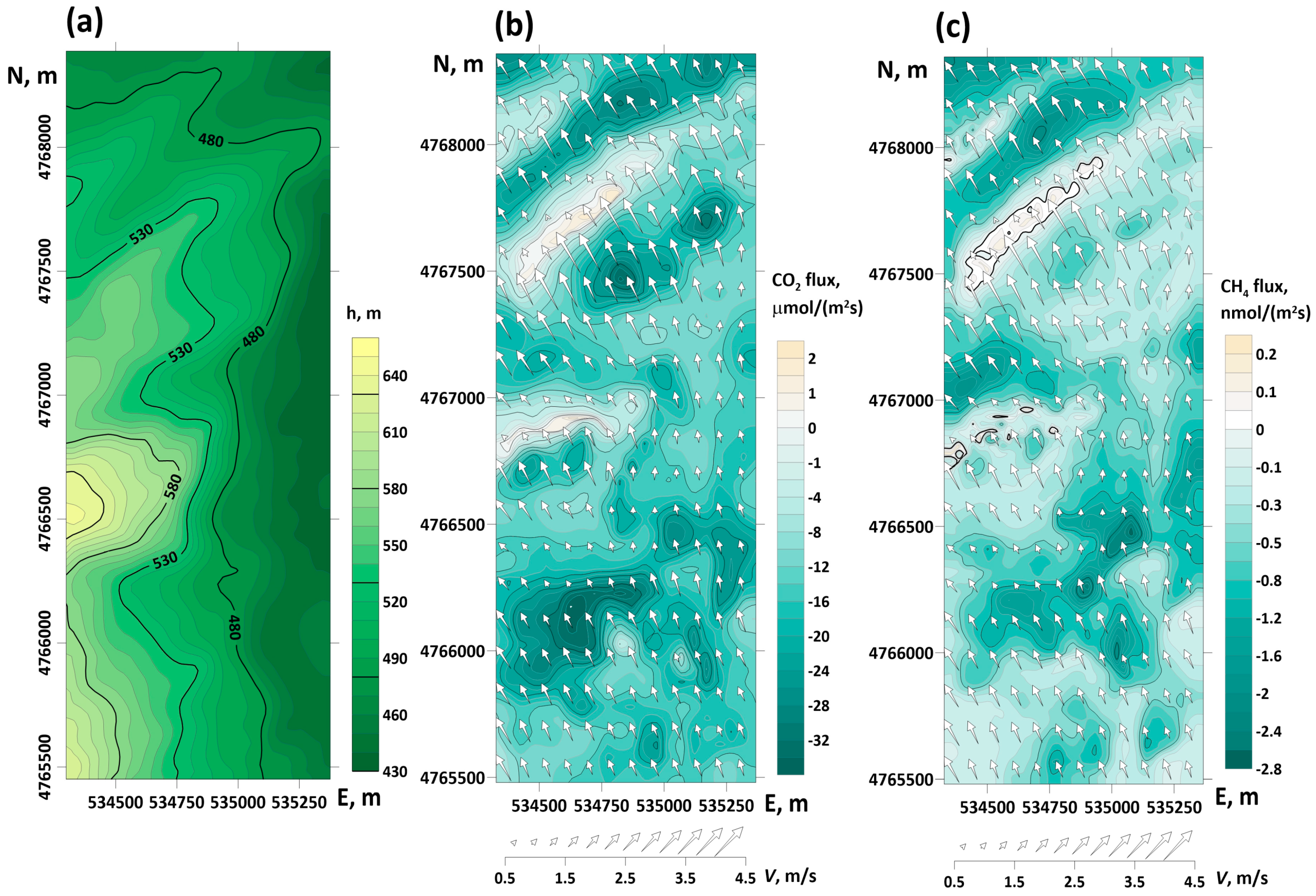
3.1. Target GHG Fluxes

For the numerical experiments, we chose a summer day with sunny weather conditions and a prevailing southeast wind direction. The topography of the model domain as well as the horizontal wind speed distribution over the study area are shown in Figure 3. As can be seen in Figure 3a, the topography of the surface within the domain varies from 430 to 660 m asl, forming several ridges of varying heights extending from southwest to northeast. The wind direction at a height of 30 m, where the GHG fluxes were determined, is nearly perpendicular to these ridges (Figure 3b,c).
The target CO2 and CH4 flux distributions simulated by model (3), which is driven by outputs from the RANS model (1) and observed GHG soil source/sink and photosynthesis data, are also shown in Figure 3. Negative flux values correspond to fluxes directed toward the ground surface, and positive values correspond to those directed outward from the surface into the atmosphere. Because the orography affects the airflow and turbulence that are responsible for the redistribution of GHGs, the pattern of the targeted fluxes depends primarily on the topography of the experimental site. The source/sink distribution is also responsible for the estimated fluxes but to a different extent for different GHGs. The CO2 sources/sinks are distributed not only horizontally but also vertically depending on the photosynthetic activity and the aerodynamic resistance of leaves at different levels within the plant canopy. It is assumed that the CH4 sources and sinks are located only on the soil surface.
Figure 3 shows that both CO2 and CH4 fluxes have increased values on windward slopes and decreased values on leeward slopes and have similar patterns. Small differences in the patterns could be due to the different vertical distributions of sources and sinks within the forest canopy. It can be seen that even at one level above the heterogeneous vegetation surface, GHG fluxes are highly variable. In this case, the positive flux values on the leeward side just behind the elevated landforms result from airflow recirculation behind the obstacle and not from the presence of a “source” of GHGs. Similar effects were found in several studies of airflow and fluxes over forested hills [57,58,59].

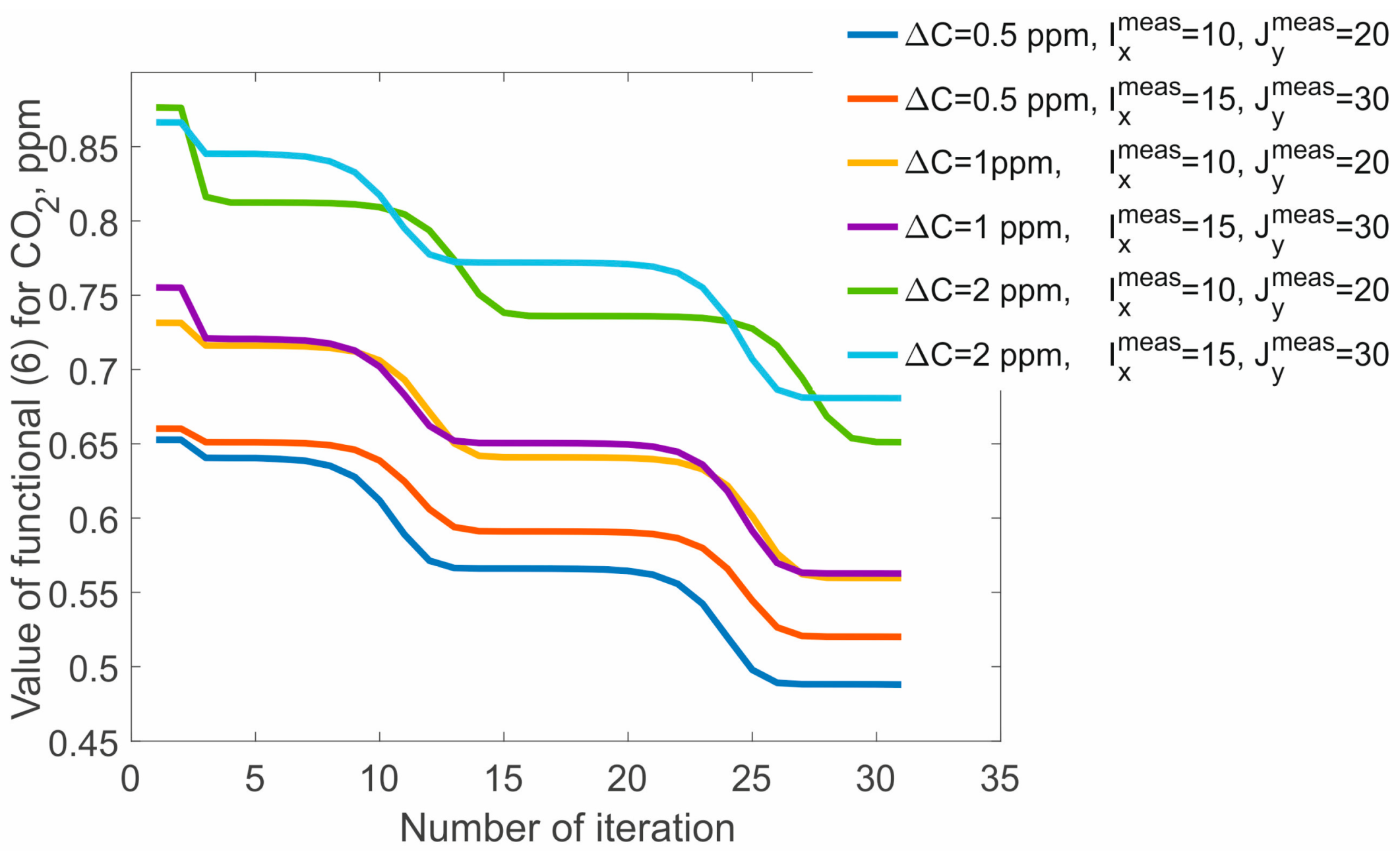
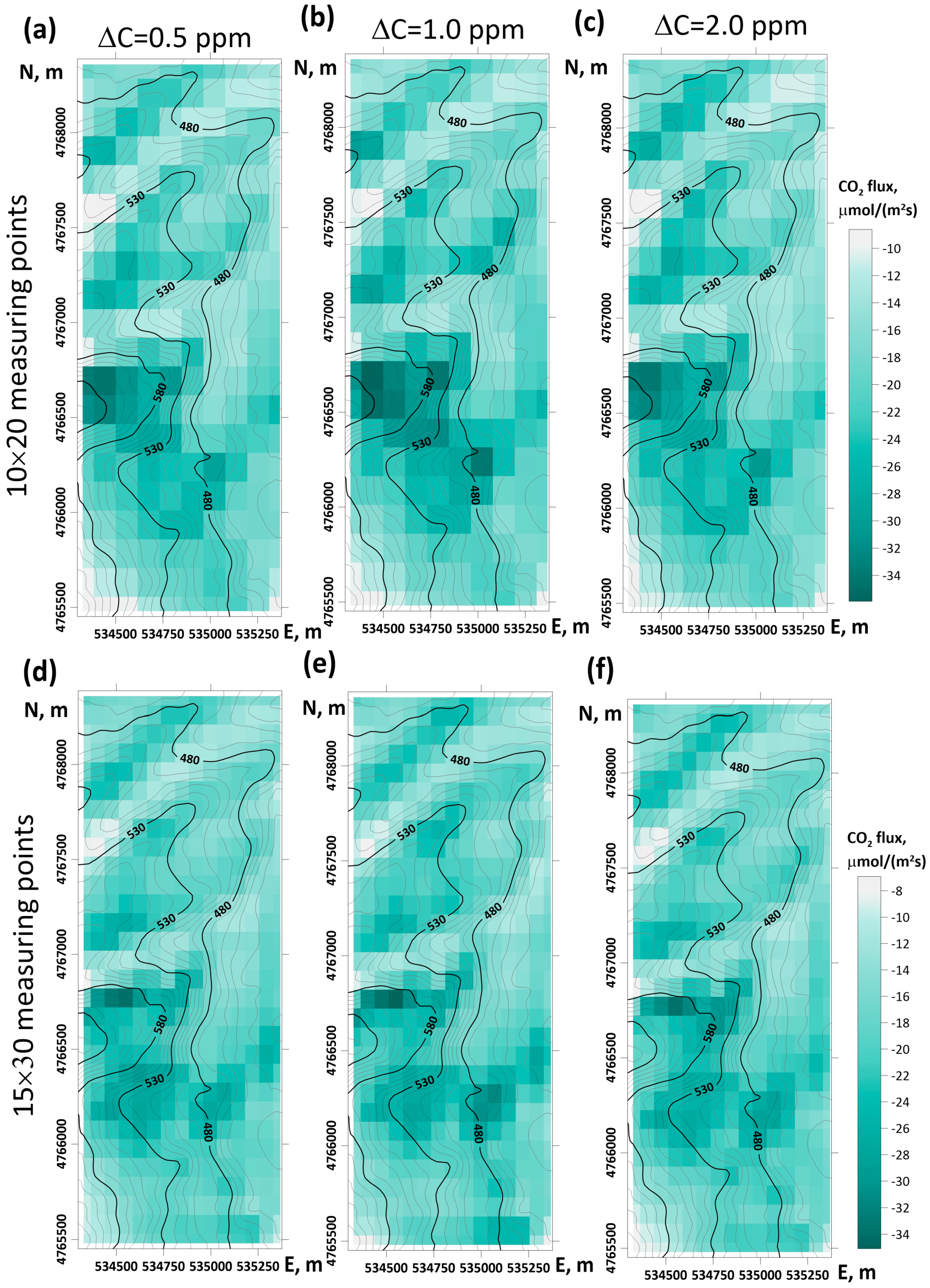
3.2. Retrieved CO2 Fluxes

Figure 4 shows the dependence of the value of the functional (6) on the number of iterations when solving the inverse problem (5) for CO2 fluxes. As can be seen in Figure 4, the iterative process is convergent in every case considered. The wave-like character of the convergence is related to the properties of the chosen minimization algorithm. To evaluate the effect of the measurement error of the concentration and the number of CO2 measurement points, we solved the inverse problem with the same number of iterations for all numerical experiments (n = 30). Considering that the convergence process requires a high computational cost, we chose this iteration value as the minimum, for which the functional value became less than the measurement error by 0.5 ppm for a 10 × 20 grid (see the dark blue line in Figure 4).
Figure 5 illustrates the CO2 fluxes at a height of 30 m above the ground, obtained using different numbers of CO2 concentration samples and different accuracies of instrumental measurements of CO2 concentrations. On the other hand, Figure 6 shows the differences between these retrieved CO2 fluxes and the target CO2 flux values at the same height. Although the retrieved CO2 fluxes accurately replicated the distribution pattern of the target CO2 fluxes (as shown in Figure 3b), there were quantitative differences between the retrieved and target fluxes (Figure 6).
Analysis of the modeling results (Figure 6) first shows that, on average, the fluxes retrieved by solving the inverse problem overestimate the mean CO2 flux by 20% in the best case considered ( Δ C = 0.5 ppm, 15 × 30 concentration measurement points) and by 30% in the worst case ( Δ C = 2 ppm, 10 × 20 concentration measurement points) (Table 1).
This overestimation of the mean CO2 flux is due to the excessive estimation of negative CO2 fluxes (uptake) in areas downwind of mountain ridges, where the target fluxes are relatively small in absolute terms and may even change their sign (Figure 5).
Since the soil flux values in the areas with the maximum overestimation of the calculated flux do not differ significantly from the flux rate in other plots of the model domain, and the LAI does not differ significantly on average over the study area (i.e., CO2 sources/sinks are more or less evenly distributed), the targeted CO2 flux distribution is mainly influenced by hydrodynamic effects caused by turbulent exchange. These effects may be underestimated in the inverse modeling due to the coarse computational grid spacing.
Secondly, there is a discrepancy between the spatial structures of the retrieved and target CO2 fluxes. The error in flux estimation was calculated as the difference between the computed fluxes at points on the measurement grid and the average of the target fluxes near those points. The target flux was averaged over cells centered on the measurement points with sides equal to twice the distance between the measurement points. The corresponding results for the CO2 fluxes are shown in Figure 6. The magnitude of the flux difference varies significantly across the modeling domain, with several maxima and minima peaks comparable to the values of the target CO2 fluxes.
After analyzing the detected flux difference and the surface topography of the experimental area (see Figure 6), several key features were identified. The maximum peak differences for all modeling experiments were found at the highest elevation points. Conversely, the areas of lowest elevation had the maximum negative anomalies. In addition, windward areas showed stronger positive flux difference anomalies, indicating an underestimation of net CO2 uptake by vegetation cover. In contrast, leeward areas showed negative anomalies, indicating a stronger net CO2 uptake.
It is also important to note that the spatial distribution of flux error maxima and minima was generally similar for all considered cases of Δ C and the number of concentration measurement points used. However, the range of minimum errors increases with the number of measurement points and the accuracy of the concentration measurements. For a more in-depth analysis of the representativeness of the results, the distributions of the deviations between the calculated and the target fluxes were also analyzed (see Figure 7 and Figure 8).
The resulting error distribution is similar enough to a normal distribution (it passes the Kolmogorov–Smirnov test). The mean error is not zero and is between 3.5 and 4 µmol/(m2s) for a modeling domain of 10 × 20 measurement points, and between 2.5 and 3 µmol/(m2s)—for 15 × 30 measurement points. The limits of the 95% confidence intervals ( q ¯ 2 σ ,   q ¯ + 2 σ ) correspond to errors in the estimation of the vertical CO₂ flux of the order of 17 μmol/(m2s) in the worst case considered ( Δ C = 2 ppm and 10 × 20 measurement points) (Figure 7c) and become narrower with an increase in the number of measurement points and an improvement in the accuracy of the concentration measurements at two levels (up to 14 μmol/(m2s) at Δ C = 0.5 ppm with 15 × 30 measurement points in our case) (Figure 7d). This means that the error decreases as the number of measurement points increases and the measurement accuracy improves. The maximum error values are in the order of 20 μmol/(m2s), which are outside the range of the 95% confidence interval of the Gaussian distribution for each case considered. These values can therefore be interpreted as outliers for the method used.
As mentioned above, the maximum errors in CO2 flux estimation for the study area were associated with areas of maximum steepness of the surface topography. Therefore, we also examined the relationship between the error and the surface slope angle (Figure 9).
Figure 9 illustrates the dependence of the accuracy of estimating the vertical CO2 flux at a height of 30 m above the ground surface on the slope angle of the terrain for different values of the measurement errors in the concentrations at two levels and a different number of samples. On average, the accuracy of flux estimation from the inverse problem solution decreases with increasing terrain slope. With more measurement points, the error is near zero for small slope angles (up to 8°). For 10 × 20 points, the average error increases with the slope angle of the surface. When the number of measurement points is increased to 15 × 30 points, the error initially increases with the slope angle and reaches a maximum of about 7.5–8 μmol/(m2s) at 20–22 degrees slopes. However, for higher slope angles, the average error decreases. It is possible that increasing the density of the grid of measurement points in areas with significant surface slopes and improving the consideration of boundary conditions in the forward problem (5) will reduce the effect of terrain on GHG emission estimates. However, further studies are needed to confirm this hypothesis.
Figure 10 summarizes the results of the sensitivity test for CO2 flux retrieval. It shows the standard deviation of the CO2 flux values obtained by inverse modeling from the target flux values as a function of the number of measurement points and the concentration measurement error at two different levels. As the number of points increases and the accuracy of the concentration measurements improves, the accuracy of the flux estimates also improves. This indicates convergence of the proposed model algorithm.

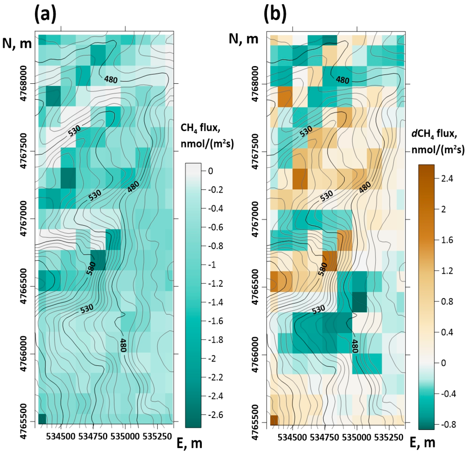
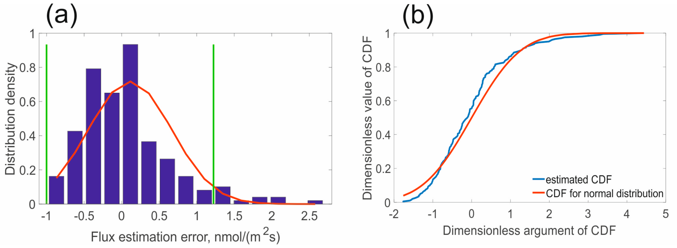
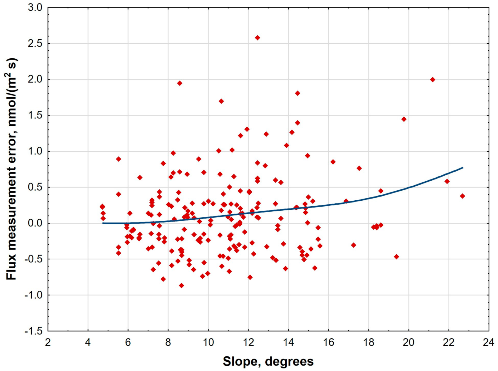
3.3. Retrieved CH4 Fluxes

When approaching the inverse problem of (5) in forward mode, i.e., with a predetermined flux at a given level h f l u x , the difference in concentration between different levels within the computational domain depends largely on the strength of the flux. Because the target CH4 flux at the level h f l u x is low intensity, the concentration difference between levels h 1 and h 2 is less than one ppb. In inverse modeling, this small difference makes minimizing the functional (6) impractical. To solve this problem, we approximate Equation (7) using finite difference and estimate the flux based on filtered measurements of CH4 concentrations at two different levels. Instead of using this estimated flux as an initial approximation, we accept it as the final solution.
Figure 11 shows the retrieved CH4 fluxes and their deviations from the target flux values for the case of 10 × 20 points and with the maximum possible error in the measured concentrations at two levels of 1 ppb. The same pattern is observed for CH4 as for CO2 with respect to the surface topography and the data samples used to retrieve the fluxes. The standard deviation of the estimated CH4 flux from the target flux is 0.56 nmol/(m2s). The mean values of the target flux and the estimated flux over the model domain are shown in Table 2.
Distributions of the deviations between the retrieved and target fluxes were calculated (see Figure 12a,b). The error distribution for the estimation of CH4 fluxes shows a more significant deviation from a Gaussian distribution than for the estimation of CO2 fluxes, although both distributions still pass the Kolmogorov–Smirnov test. This difference is due to the different procedures used to derive the fluxes from the concentration measurements. When estimating CO2 fluxes, minimizing the functional leads to error statistics that accumulate in such a way that the error distribution gets closer to a Gaussian distribution.
Figure 13 illustrates the accuracy of estimating vertical CH4 fluxes at 30 m above the surface as a function of site slope. Unlike CO2 fluxes, the accuracy of CH4 fluxes is not significantly affected by site slope due to the different distributions of CH4 sources and sinks within the plant canopy and soil. The effect of soil CH4 sources and sinks on the resulting CH4 flux at 30 m is probably masked by the turbulent regime within the canopy layer that separates the soil surface from the reference level within the atmospheric boundary layer. The error slowly increases when the slope of the surface exceeds 16 degrees. Overall, we can ignore the effect of topography on the accuracy of the retrieved CH4 flux in the considered study area.

4. Conclusions

We have proposed a modeling approach for estimating GHG fluxes between the Earth’s surface and the atmosphere in various terrain types using UAV measurements of their concentrations in the ABL. Briefly, the proposed approach includes the following steps:
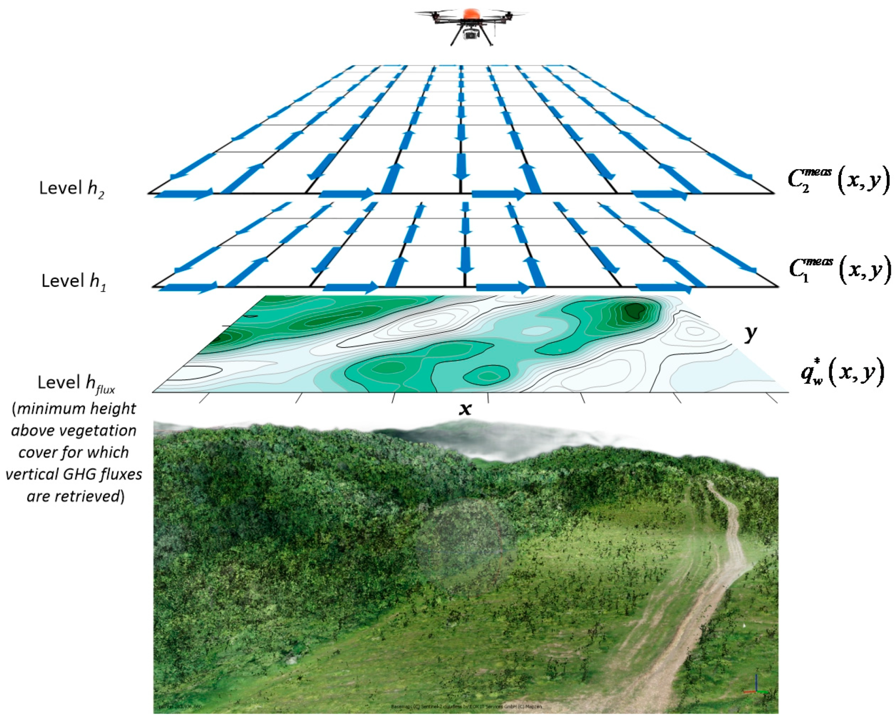
  • Collecting concentration data over complex terrain at two levels within the atmospheric surface layer with some spatial resolution.
  • Estimating airflow characteristics over the study area that can be measured directly by the UAV or derived from the ABL model.
  • Making a first approximation of the GHG flux distribution over the area of interest q w i n i x , y , h x , y + h f l u x using the collected concentrations and estimated airflow characteristics.
  • Deriving the required distribution of vertical fluxes q w x , y by solving the inverse problem (5) multiple times with intentionally varying function q w x , y , h x , y + h f l u x as input data. The solution is achieved by minimizing functional (6).
To test the algorithm, we performed numerical experiments initialized with surrogate concentration data of varying quality, including different measurement errors and density of measurements.
The model experiments show that the accuracy of the retrieved fluxes depends on the initial measurement error and thus on the measurement quality. Even with a coarse measurement grid, the estimated fluxes remain close to the target values. It should be noted that all experiments were performed under identical airflow conditions. Therefore, the effect of turbulence parameters on the quality of the flux retrievals was not taken into account. However, it can be assumed that improving the description of the airflow by refining the computational grid will lead to enhanced results. This assumption is supported by the fact that the quality-derived results depend on the slope of the terrain.
In our test study, we used a uniform grid of measurement points unsuited to the terrain’s complexity. Nevertheless, the results were satisfactory, and the maximum error values can be considered as outliers of the method. Future research will aim to reduce errors by refining the grid in areas with steep slopes, improving the accuracy of the boundary condition approximation in problem (5), and adjusting the vertical grid spacing.
The novelty of our approach lies in the use of the ABL model to describe a turbulent condition over a non-uniform underlying surface that is responsible for the redistribution of GHGs and, as a result, for the vertical fluxes of GHGs. The application of the ABL model gives our approach an advantage over others based on analytical or empirical descriptions of atmospheric turbulent conditions because it is able to adequately describe vertical GHG fluxes over non-uniform landscapes with complex topography and mosaic vegetation. Its potential disadvantage is the need for detailed information on the characteristics of the study area, such as surface topography, vegetation characteristics, etc. Inverse modeling can also be time-consuming in the case of strong landscape heterogeneity and many GHG measurement points.
The proposed algorithm shows promise as a first step towards developing a tool for performing UAV measurements over complex terrain. The next step is to test the algorithm using actual UAV measurements.

Author Contributions

Conceptualization, I.M. and A.S.; methodology, I.M. and A.S.; software, I.M.; validation, I.M.; formal analysis, I.M. and R.G.; investigation, I.M., R.G. and V.P.; data curation, I.M.; data analysis, I.M., R.G. and V.P.; writing—original draft preparation, A.S., I.M. and A.O.; writing—review and editing, A.O., A.S. and I.M.; visualization, I.M., A.O. and R.G.; supervision, A.O.; project administration, I.A.K. and A.O.; funding acquisition, I.A.K. All authors have read and agreed to the published version of the manuscript.

Funding

Analysis of modeling results provided by A. Sogachev was supported by a state assignment of the Ministry of Science and High Education of the Russian Federation FFER-2022-0002 (theme no. 1022031600002-1-1.6.19). The field measurements at the Roshny-Chu forest site and modeling experiments were supported by the State Assignment of the Grozny State Oil Technical University (Project Reg. No. FZNU-2024-0002). The conceptual design of the study was supported by the Government of the Tyumen region within the framework of the Program of the World-Class West Siberian Interregional Scientific and Educational Center (National project “Nauka”).

Data Availability Statement

The original contributions presented in the study are included in the article, further inquiries can be directed to the corresponding author/s.

Conflicts of Interest

The authors declare no conflicts of interest.

References

  1. Pörtner, H.O.; Roberts, D.C.; Tignor, M.; Poloczanska, E.S.; Mintenbeck, K.; Alegría, A.; Craig, M.; Langsdorf, S.; Löschke, S.; Möller, V.; et al. (Eds.) IPCC, 2022: Climate Change 2022: Impacts, Adaptation, and Vulnerability; Contribution of Working Group II to the Sixth Assessment Report of the Intergovernmental Panel on Climate Change; Cambridge University Press: Cambridge, UK; New York, NY, USA, 2022; p. 3056. [Google Scholar]
  2. Yue, X.L.; Gao, Q.X. Contributions of natural systems and human activity to greenhouse gas emissions. Adv. Clim. Change Res. 2018, 9, 243–252. [Google Scholar] [CrossRef]
  3. Friedlingstein, P.; O’Sullivan, M.; Jones, M.W.; Andrew, R.M.; Bakker, D.C.E.; Hauck, J.; Landschützer, P.; Le Quéré, C.; Luijkx, I.T.; Peters, G.P.; et al. Global Carbon Budget. Earth Syst. Sci. Data. 2023, 15, 5301–5369. [Google Scholar] [CrossRef]
  4. Aubinet, M.; Vesala, T.; Papale, D. Eddy Covariance: A Practical Guide to Measurement and Data Analysis; Springer: Dordrecht, The Netherlands, 2012; p. 438. [Google Scholar]
  5. Baldocchi, D.; Hicks, B.; Meyers, T. Measuring biosphere—Atmosphere exchanges of biologically related gases with micrometeorological methods. Ecology 1988, 69, 1331–1340. [Google Scholar] [CrossRef]
  6. Foken, T.; Wichura, B. Tools for quality assessment of surface-based flux measurements. Agric. For. Meteorol. 1996, 78, 83–105. [Google Scholar] [CrossRef]
  7. Ibrom, A.; Schütz, C.; Tworek, T.; Morgenstern, K.; Oltchev, A.; Falk, M.; Constantin, J.; Gravenhorst, G. Eddy-correlation measurements of fluxes of CO2 and H2O above a spruce forest. J. Phys. Chem. Earth 1996, 21, 409–414. [Google Scholar] [CrossRef]
  8. Jägermeyr, J.; Gerten, D.; Lucht, W.; Hostert, P.; Migliavacca, M.; Nemani, R. A high-resolution approach to estimating ecosystem respiration at continental scales using operational satellite data. Glob. Change Biol. 2014, 20, 1191–1210. [Google Scholar] [CrossRef] [PubMed]
  9. Junttila, S.; Kelly, J.; Kljun, N.; Aurela, M.; Klemedtsson, L.; Lohila, A.; Nilsson, M.B.; Rinne, J.; Tuittila, E.-S.; Vestin, P.; et al. Upscaling northern peatland CO2 fluxes using satellite remote sensing data. Remote Sens. 2021, 13, 818. [Google Scholar] [CrossRef]
  10. Wang, S.; Garcia, M.; Ibrom, A.; Bauer-Gottwein, P. Temporal interpolation of land surface fluxes derived from remote sensing—Results with an unmanned aerial system. Hydrol. Earth Syst. Sci. 2020, 24, 3643–3661. [Google Scholar] [CrossRef]
  11. Bolek, A.; Heimann, M.; Göckede, M. UAV based in situ measurements of CO2 and CH4 fluxes over complex natural ecosystems. Atmos. Meas. Tech. Discuss. 2024, 2024, 27. [Google Scholar]
  12. Baldocchi, D.; Falge, E.; Gu, L.; Olson, R.; Hollinger, D.; Running, S.; Anthoni, P.; Bernhofer, C.; Davis, K.; Evans, R.; et al. FLUXNET: A new tool to study the temporal and spatial variability of ecosystem-scale carbon dioxide, water vapor and energy flux densities. Bull. Am. Meteorol. Soc. 2001, 82, 2415–2434. [Google Scholar] [CrossRef]
  13. Papale, D.; Black, T.A.; Carvalhais, N.; Cescatti, A.; Chen, J.; Jung, M.; Kiely, G.; Lasslop, G.; Mahecha, M.; Margolis, H.; et al. Effect of spatial sampling from European flux towers for estimating carbon and water fluxes with artificial neural networks. J. Geophys. Res. Biogeosci. 2015, 120, 1941–1957. [Google Scholar] [CrossRef]
  14. Baldocchi, D. How eddy covariance flux measurements have contributed to our understanding of Global Change Biology. Glob. Change Biol. 2020, 26, 242–260. [Google Scholar] [CrossRef] [PubMed]
  15. Villarreal, S.; Vargas, R. Representativeness of FLUXNET sites across Latin America. J. Geophys. Res. Biogeosci. 2021, 126, 1–18. [Google Scholar] [CrossRef]
  16. Foken, T. The energy balance closure problem: An overview. Ecol. Appl. 2008, 18, 1351–1367. [Google Scholar] [CrossRef] [PubMed]
  17. Pumpanen, J.; Kolari, P.; Ilvesniemi, H.; Minkkinen, K.; Vesala, T.; Niinisto, S.; Lohila, A.; Larmola, T.; Morero, M.; Pihlatie, M.; et al. Comparison of different chamber techniques for measuring soil CO2 efflux. Agric. For. Meteorol. 2004, 123, 159–176. [Google Scholar] [CrossRef]
  18. Olchev, A.; Volkova, E.; Karataeva, T.; Novenko, E. Growing season variability of net ecosystem CO2 exchange and evapotranspiration of a sphagnum mire in the broad-leaved forest zone of European Russia. Environ. Res. Lett. 2013, 8, 035051. [Google Scholar] [CrossRef]
  19. Molchanov, A.G.; Kurbatova, Y.A.; Olchev, A.V. Effect of Clear-Cutting on Soil CO2 Emission. Biol. Bull. 2017, 44, 218–223. [Google Scholar] [CrossRef]
  20. Mohren, G.M.J.; Hasenauer, H.; Köhl, M.; Nabuurs, G.J. Forest inventories for carbon change assessments. Curr. Opin. Environ. Sustain. 2012, 4, 686–695. [Google Scholar] [CrossRef]
  21. Deng, Z.; Ciais, P.; Tzompa-Sosa, Z.A.; Saunois, M.; Qiu, C.; Tan, C.; Sun, T.; Ke, P.; Cui, Y.; Tanaka, K.; et al. Comparing national greenhouse gas budgets reported in UNFCCC inventories against atmospheric inversions. Earth Syst. Sci. Data 2021, 14, 1639–1675. [Google Scholar] [CrossRef]
  22. Li, C.; Han, W.; Peng, M. Improving the spatial and temporal estimating of daytime variation in maize net primary production using unmanned aerial vehicle-based remote sensing. Int. J. Appl. Earth Obs. Geoinf. 2021, 103, 102467. [Google Scholar] [CrossRef]
  23. Nasiri, V.; Darvishsefat, A.A.; Arefi, H.; Pierrot-Deseilligny, M.; Namiranian, M.; Le Bris, A. Unmanned aerial vehicles (UAV)-based canopy height modeling under leaf-on and leaf-off conditions for determining tree height and crown diameter (case study: Hyrcanian mixed forest). Can. J. For. Res. 2021, 51, 962–971. [Google Scholar] [CrossRef]
  24. Pourreza, M.; Moradi, F.; Khosravi, M.; Deljouei, A.; Vanderhoof, M.K. GCPs-Free Photogrammetry for Estimating Tree Height and Crown Diameter in Arizona Cypress Plantation Using UAV-Mounted GNSS RTK. Forests 2022, 13, 1905. [Google Scholar] [CrossRef]
  25. Elston, J.; Argrow, B.; Stachura, M.; Weibel, D.; Lawrence, D.; Pope, D. Overview of small fixed-wing unmanned aircraft for meteorological sampling. J. Atmos. Ocean Technol. 2015, 32, 97–115. [Google Scholar] [CrossRef]
  26. Jacob, J.D.; Chilson, P.B.; Houston, A.L.; Smith, S.W. Considerations for atmospheric measurements with small unmanned aircraft systems. Atmosphere 2018, 9, 252. [Google Scholar] [CrossRef]
  27. Barbieri, L.; Kral, S.T.; Bailey, S.C.C.; Frazier, A.E.; Jacob, J.D.; Reuder, J.; Brus, D.; Chilson, P.B.; Crick, C.; Detweiler, C.; et al. Intercomparison of small unmanned aircraft system (sUAS) measurements for atmospheric science during the LAPSE-RATE campaign. Sensors 2019, 19, 2179. [Google Scholar] [CrossRef] [PubMed]
  28. Shaw, J.T.; Shah, A.; Yong, H.; Allen, G. Methods for quantifying methane emissions using unmanned aerial vehicles: A review. Phil. Trans. R. Soc. 2021, 379, 1–21. [Google Scholar] [CrossRef] [PubMed]
  29. Kunz, M.; Lavric, J.V.; Gasche, R.; Gerbig, C.; Grant, R.H.; Koch, F.T.; Schumacher, M.; Wolf, B.; Zeeman, M. Surface flux estimates derived from UAS-based mole fraction measurements by means of a nocturnal boundary layer budget approach. Atmos. Meas. Tech. 2020, 13, 1671–1692. [Google Scholar] [CrossRef]
  30. Reuter, M.; Bovensmann, H.; Buchwitz, M.; Borchardt, J.; Krautwurst, S.; Gerilowski, K.; Lindauer, M.; Kubistin, D.; Burrows, J.P. Development of a small unmanned aircraft system to derive CO2 emissions of anthropogenic point sources. Atmos. Meas. Tech. 2021, 14, 153–172. [Google Scholar]
  31. Wang, J.; Feng, L.; Palmer, P.I.; Liu, Y.; Fang, S.; Bösch, H.; O’Dell, C.; Tang, X.; Yang, D.; Liu, L.; et al. Large Chinese land carbon sink estimated from atmospheric carbon dioxide data. Nature 2020, 586, 720–723. [Google Scholar] [CrossRef] [PubMed]
  32. Hutchinson, M.; Oh, H.; Chen, W.-H. A review of source term estimation methods for atmospheric dispersion events using static or mobile sensors. Inf. Fusion 2017, 36, 130–148. [Google Scholar] [CrossRef]
  33. Ristic, B.; Gilliam, C.; Moran, W.; Palmer, J.L. Decentralized multi-platform search for a hazardous source in a turbulent flow. Inf. Fusion 2020, 58, 13–23. [Google Scholar] [CrossRef]
  34. Allen, G.; Hollingsworth, P.; Kabbabe, K.; Pitt, J.R.; Mead, M.I.; Illingworth, S.; Roberts, G.; Bourn, M.; Shallcross, D.E.; Percival, C.J. The development and trial of an unmanned aerial system for the measurement of methane flux from landfill and greenhouse gas emission hotspots. Waste Manag. 2019, 87, 883–892. [Google Scholar] [CrossRef] [PubMed]
  35. Pirk, N.; Aalstad, K.; Westermann, S.; Vatne, A.; van Hove, A.; Tallaksen, L.M.; Cassiani, M.; Katul, G. Inferring surface energy fluxes using drone data assimilation in large eddy simulations. Atmos. Meas. Tech. 2022, 15, 7293–7314. [Google Scholar] [CrossRef]
  36. Carbon Supersites. Available online: https://carbon-polygons.ru/en/ (accessed on 29 April 2024).
  37. Mukhartova, I.; Kurbatova, J.; Tarasov, D.; Gibadullin, R.; Sogachev, A.; Olchev, A. Modeling tool for estimating carbon dioxide fluxes over a non-uniform boreal peatland. Atmosphere 2023, 14, 625. [Google Scholar] [CrossRef]
  38. Mukhartova, Y.; Levashova, N.; Olchev, A.; Shapkina, N. Application of a 2D model for describing the turbulent transfer of CO2 in a spatially heterogeneous vegetation cover. Mosc. Univ. Phys. Bull. 2015, 70, 14–21. [Google Scholar] [CrossRef]
  39. Mukhartova, Y.; Dyachenko, M.; Mangura, P.; Mamkin, V.; Kurbatova, J.; Olchev, A. Application of a three-dimensional model to assess the effect of clear-cutting on carbon dioxide exchange at the soil—Vegetation—Atmosphere interface. IOP Conf. Ser. Earth Environ. Sci. 2019, 368, 012036. [Google Scholar] [CrossRef]
  40. Sogachev, A.; Kelly, M.; Leclerc, M.Y. Consistent Two-Equation Closure Modelling for Atmospheric Research: Buoyancy and Vegetation Implementations. Bound. Layer Meteorol. 2012, 145, 307–327. [Google Scholar] [CrossRef]
  41. Allen, T.; Zerroukat, M. A simple immersed boundary forcing for flows over steep and complex orography. Q. J. R. Meteorol Soc. 2020, 146, 3488–3502. [Google Scholar] [CrossRef]
  42. Stull, R.B. An Introduction to Boundary Layer Meteorology; Kluwer Academic Publishers: Dordrecht, The Netherlands, 1998; p. 666. [Google Scholar]
  43. Sogachev, A.; Menzhulin, G.V.; Heimann, M.; Lloyd, J. A simple three-dimensional canopy-planetary boundary layer simulatiom model for scalar concentrations and fluxes. Tellus 2002, 54, 784–819. [Google Scholar]
  44. Sogachev, A.; Panferov, O. Modification of two-equation models to account for plant drug. Bound. Layer Meteorol. 2006, 121, 229–266. [Google Scholar] [CrossRef]
  45. Garratt, J.R. The Atmospheric Boundary Layer; Cambridge University press: Cambridge, UK, 1992; p. 316. [Google Scholar]
  46. Foken, T. Micrometeorology; Springer-Verlag Publishers: Berlin/Heidelberg, Germany, 2008; p. 306. [Google Scholar]
  47. Blanken, P.D.; Williams, M.W.; Burns, S.P.; Monson, R.K.; Knowles, J.; Chowanski, K.; Ackerman, T. A comparison of water and carbon dioxide exchange at a windy alpine tundra and subalpine forest site near Niwot Ridge, Colorado. Biogeochemistry 2009, 95, 61–76. [Google Scholar] [CrossRef]
  48. Feigenwinter, C.; Bernhofer, C.; Eichelmann, U.; Heinesch, B.; Hertel, M.; Janous, D.; Kolle, O.; Lagergren, F.; Lindroth, A.; Minerbi, S.; et al. Comparison of horizontal and vertical advective CO2 fluxes at three forest sites. Agric. For. Meteorol. 2008, 148, 12–24. [Google Scholar] [CrossRef]
  49. Leuning, R.; Zegelin, S.J.; Jones, K.; Keith, H.; Hughes, D. Measurement of horizontal and vertical advection of CO2 within a forest canopy. Agric. For. Meteorol. 2008, 148, 1777–1797. [Google Scholar] [CrossRef]
  50. Mukhartova, I.V.; Olchev, A.V.; Gibadullin, R.R.; Lukyanenko, D.V.; Makmudova, L.S.; Kerimov, I.A. Inverse problem for retrieving greenhouse gas fluxes at the non-uniform underlying surface from measurements of their concentrations at several levels. J. Phys. Conf. Ser. 2024, 2701, 012141. [Google Scholar] [CrossRef]
  51. Olchev, A.V.; Mukhartova, I.V.; Kerimov, I.A.; Gibadullin, R.R. 3D Hydrodynamic Modeling of CO2 and CH4 Fluxes in the Atmospheric Surface Layer (example of the Roshni-chu Forest Site). Sustain. Dev. Mt. Territ. 2023, 15, 408–418. [Google Scholar] [CrossRef]
  52. Peel, M.C.; Finlayson, B.L.; McMahon, T.A. Updated world map of the Koppen-Geiger climate classification. Hydrol. Earth Syst. Sci. 2007, 11, 1633–1644. [Google Scholar] [CrossRef]
  53. Pridacha, V.B.; Makhmudova, L.S.; Semin, D.E.; Olchev, A.V. Photosynthetic Parameters of the Woody Plant Species in the in the Foothills of Northern Caucasian Broadleaved Forests. Grozny Nat. Sci. Bull. 2022, 7, 105–112. [Google Scholar]
  54. Kerimov, I.A.; Ezirbaev, T.B. Experiences in the Application of Multispectral Imagery in Land Cover Observation. Ecol. Environ. Prot. Carbon Neutrality Dev. 2022, 12, 182–193. [Google Scholar]
  55. Olchev, A.; Radler, K.; Sogachev, A.; Panferov, O.; Gravenhorst, G. Application of a three-dimensional model for assessing effects of small clear-cuttings on radiation and soil temperature. Ecol. Model. 2009, 220, 3046–3056. [Google Scholar] [CrossRef]
  56. Nocedal, J.; Öztoprak, F.; Waltz, R.A. An interior point method for nonlinear programming with infeasibility detection capabilitie. Optim. Methods Softw. 2014, 29, 837–854. [Google Scholar] [CrossRef]
  57. Finnigan, J.J.; Belcher, S.E. Flow over a hill covered with a plant canopy. Q. J. Roy. Meteorol. Soc. 2004, 130, 1–29. [Google Scholar] [CrossRef]
  58. Dupont, S.; Brunet, Y.; Finnigan, J. Large-eddy simulation of turbulent flow over a forested hill: Validation and coherent structure identification. Q. J. Roy. Meteorol. Soc. 2008, 134, 1911–1929. [Google Scholar] [CrossRef]
  59. Liu, Z.; Hu, Y.; Fan, Y.; Wang, W.; Zhou, Q. Turbulent flow fields over a 3D hill covered by vegetation canopy through large eddy simulations. Energies 2019, 12, 3624. [Google Scholar] [CrossRef]
Figure 1. Altitude level scheme for retrieving GHG fluxes q w x , y from UAV GHG concentration measurements C k m e a s x , y . See the text for details.
Remotesensing 16 02502 g001
Figure 2. Geographical location of the study area (a) and UAV-derived 3D view of the experimental site’s topography and LAI distribution (b). The surface topography map is created using the UTM coordinate system, 38T (WGS84).
Remotesensing 16 02502 g002
Figure 3. Surface topography within the study area (a) and target turbulent vertical CO2 (b) and CH4 (c) fluxes at a height of 30 m above the ground. The white arrows indicate the wind direction and wind speed at the selected height.
Remotesensing 16 02502 g003
Figure 4. Dependencies of the values of the functional (6) minimized in the solution of the inverse problem on the number of iterations: values of the functional (6) for CO2 at different numbers of measuring points and different errors of concentration measurement at two levels.
Remotesensing 16 02502 g004
Figure 5. Retrieved from inverse modeling of vertical CO2 fluxes at a height of 30 m above the ground. The fluxes are shown as a function of the maximum measurement errors ( Δ C ) and the number of CO2 concentration measurement points at each level I x m e a s , J y m e a s . Columns (a,d), (b,e), and (c,f) show modeling results considering different measurement errors Δ C = 0.5, 1, and 2 ppm, respectively. The panels (ac) and (df) represent results for the different number of measurement points (10 × 20) and (15 × 30), respectively. The CO2 concentration measurement points at different levels have the same horizontal coordinates (positioned one above the other). The black isolines show the surface topography.
Remotesensing 16 02502 g005
Figure 6. Deviation of the retrieved vertical CO2 flux from the target CO2 fluxes for the same cases as in Figure 5. Columns (a,d), (b,e), and (c,f) show modeling results considering different measurement errors Δ C = 0.5, 1, and 2 ppm, respectively. The panels (ac) and (df) represent results for the different number of measurement points (10 × 20) and (15 × 30), respectively. The black isolines show the surface topography.
Remotesensing 16 02502 g006
Figure 7. The distributions of vertical CO2 flux estimation errors at a height of 30 m above the ground, obtained by inverse modeling of the target CO2 concentration values. The columns represent different concentration measurement errors (0.5 ppm (a,d), 1 ppm (b,e), and 2 ppm (c,f), respectively), and the panels represent the number of points (10 × 20 (ac) and 15 × 30 (df)). The histograms correspond to the distributions of the calculated error, the red line shows the corresponding Gaussian distribution, and the vertical green lines represent the “2σ-interval”.
Remotesensing 16 02502 g007
Figure 8. Cumulative distribution functions (CDFs) of vertical CO2 flux estimation errors at a height of 30 m above the ground, obtained by inverse modeling of the target CO2 concentration values. Columns represent different concentration measurement errors (0.5 ppm (a,d), 1 ppm (b,e), and 2 ppm (c,f), respectively), and panels represent the number of measurement points (10 × 20 (ac) and 15 × 30 (df)).
Remotesensing 16 02502 g008
Figure 9. The dependence of vertical CO2 flux estimation errors on the surface slope angle. The columns represent different concentration measurement errors (0.5 (a,d), 1 (b,e), and 2 (c,f) ppm, respectively), and the panels represent the number of points (10 × 20 (ac) and 15 × 30 (df)). The red dots correspond to the calculated error values and the blue line represents the result of the least-squares smoothing.
Remotesensing 16 02502 g009
Figure 10. The standard deviations (SDs) of the CO2 flux values obtained from the inverse modeling of the target flux at a 30 m height as a function of the number of measurement points and the measurement errors of the CO2 concentration.
Remotesensing 16 02502 g010
Figure 11. Estimated vertical CH4 fluxes at a height of 30 m above the ground (a) and deviations of the vertical CH4 fluxes from the target fluxes (b). The black isolines show the surface topography.
Remotesensing 16 02502 g011
Figure 12. Distribution of vertical CH4 flux estimation errors at a height of 30 m above ground (a) and the corresponding cumulative distribution function (b) obtained for measurement errors of 1 ppb and 10 × 20 points. The histogram in (a) corresponds to the calculated error distribution, the red line shows the corresponding Gaussian distribution, and the vertical green lines represent the “2σ-interval”.
Remotesensing 16 02502 g012
Figure 13. The dependence of the vertical CH4 flux estimation errors on the slope surface angle for concentration measurement errors (1 ppb) and the number of measurement points (10 × 20). The red dots correspond to the calculated error values and the blue line represents the result of the least-squares smoothing.
Remotesensing 16 02502 g013
Table 1. Area-averaged target CO2 flux and the fluxes retrieved by inverse modeling.
Fluxes Mean Value, µmol/(m2s)
Target flux−15.34
Retrieved flux for ΔC = 0.5 ppm and 10 × 20 data points−19.01
Retrieved flux ΔC = 1 ppm, 10 × 20 data points−19.17
Retrieved flux ΔC = 2 ppm, 10 × 20 data points−19.88
Retrieved flux ΔC = 0.5 ppm, 15 × 30 data points−18.35
Retrieved flux ΔC = 1 ppm, 15 × 30 data points−18.40
Retrieved flux ΔC = 2 ppm, 15 × 30 data points−18.68
Table 2. Area-averaged target CH4 flux and flux retrieved by inverse modeling.
FluxesMean Value, nmol/(m2s)
Target flux−0.59
Retrieved flux for ΔC = 1 ppb and 10 × 20 data points−0.69
Disclaimer/Publisher’s Note: The statements, opinions and data contained in all publications are solely those of the individual author(s) and contributor(s) and not of MDPI and/or the editor(s). MDPI and/or the editor(s) disclaim responsibility for any injury to people or property resulting from any ideas, methods, instructions or products referred to in the content.

