Article

North American Circum-Arctic Permafrost Degradation Observation Using Sentinel-1 InSAR Data

1
Aerospace Information Research Institute, Chinese Academy of Sciences, Beijing 100094, China
2
International Research Center of Big Data for Sustainable Development Goals, Beijing 100094, China
3
University of Chinese Academy of Sciences, Beijing 100049, China
*
Author to whom correspondence should be addressed.
Remote Sens. 2024, 16(15), 2809; https://doi.org/10.3390/rs16152809
Submission received: 6 June 2024 / Revised: 22 July 2024 / Accepted: 29 July 2024 / Published: 31 July 2024
(This article belongs to the Special Issue Remote Sensing of the Cryosphere II)

Abstract

:
In the context of global warming, the accelerated degradation of circum-Arctic permafrost is releasing a significant amount of carbon. InSAR can indirectly reflect the degradation of permafrost by monitoring its deformation. This study selected three typical permafrost regions in North America: Alaskan North Slope, Northern Great Bear Lake, and Southern Angikuni Lake. These regions encompass a range of permafrost landscapes, from tundra to needleleaf forests and lichen-moss, and we used Sentinel-1 SAR data from 2018 to 2021 to determine their deformation. In the InSAR process, due to the prolonged snow cover in the circum-Arctic permafrost, we used only SAR data collected during the summer and applied a two-stage interferogram selection strategy to mitigate the resulting temporal decorrelation. The Alaskan North Slope showed pronounced subsidence along the coastal alluvial plains and uplift in areas with drained thermokarst lake basins. Northern Great Bear Lake, which was impacted by wildfires, exhibited accelerated subsidence rates, revealing the profound and lasting impact of wildfires on permafrost degradation. Southern Angikuni Lake’s lichen and moss terrains displayed mild subsidence. Our InSAR results indicate that more than one-third of the permafrost in the North American study area is degrading and that permafrost in diverse landscapes has different deformation patterns. When monitoring the degradation of large-scale permafrost, it is crucial to consider the unique characteristics of each landscape.

1. Introduction

Permafrost refers to ground where temperatures have remained at or below 0 °C for two consecutive years or more. According to previous studies, permafrost covers about 11% to 15% of the Arctic and northern regions, and it accounts for 15% to 24% of the northern hemisphere [1,2]. In recent years, the problem of global warming has intensified, with the Arctic warming more rapidly than any other region on Earth [3,4]. Consequently, a substantial portion of permafrost in the Northern Hemisphere is projected to warm and thaw, transitioning from a carbon sink to a carbon source [5,6,7]. This transformation is anticipated to have profound environmental and climatic impacts both within permafrost-covered regions and globally. Warming and degradation of the near-surface permafrost table can result in surface subsidence in ice-rich permafrost regions, contribute to the development of thermokarst landscapes, trigger slope instability, and cause infrastructure damage. The thawing of organic-rich permafrost has particularly positive feedback effects on climate warming as it releases a substantial amount of soil organic carbon [8,9]. Seasonal freeze–thaw cycles are the main manifestation of surface deformation in permafrost areas, typically including surface subsidence during the summer thawing season and surface uplift during the winter frost season [10]. If the long-term trend is characterized by a consistent seasonal thaw in summer, it will result in effective subsidence in long-term permafrost observations, enabling the inference of permafrost degradation [11].
The Interferometric Synthetic Aperture Radar (InSAR) technique has been widely used in studying the characteristics of ground surface deformation caused by seasonal upward and downward motion in permafrost regions [12,13,14]. This is attributed to its numerous advantages, including the ability to observe a large area and achieve high accuracy [15,16,17,18]. Subtle changes in ground subsidence and heave, ranging from millimeters to centimeters, can be accurately captured by measuring the phase difference of radar signals, which can then be converted into line-of-sight (LOS) displacement. Numerous studies have demonstrated the utility of InSAR technology in observing ground motion related to the freeze–thaw cycle in Arctic permafrost regions. For example, in the Prudhoe Bay area of northern Alaska, data from the European Remote-Sensing Satellite-1 (ERS-1) and Advanced Land Observing Satellite (ALOS) were used to monitor both seasonal thaw settlement and long-term subsidence over permafrost [10,19]. InSAR captured surface subsidence resulting from the 2014 Anaktuvuk River wildfire in northern Alaska. This subsidence was attributed to a combination of factors, including the thickening of the active layer and settlement due to permafrost thawing [20]. Sentinel-1 data from 2016 and 2017 were utilized to monitor summer surface displacement in the local area of Teshekpuk Lake, Alaska [21]. Additionally, in northern Canada, RADARSAT-2 data were utilized to assess thaw settlement at Iqaluit Airport on Baffin Island, complemented by comparative analysis against field data [22]. In the discontinuous permafrost region on the eastern shore of Hudson Bay, a combination of Sentinel-1, TerraSAR-X, and ALOS PALSAR data enabled the identification of coherent characteristics and distinct displacement patterns in various land covers within the subarctic tundra environment [23].
Some of these studies have highlighted the challenges associated with long-term continuous observation of surface deformation in permafrost terrains. When using InSAR for surface deformation detection, the typical challenges include atmospheric disturbances [24], residual topographic errors, and temporal and spatial decorrelation [17,21,25]. The Small Baseline Subset (SBAS) method employs interferograms with small temporal and spatial baselines, stacking them to obtain higher-quality interferograms to obtain cumulative deformation and deformation rates [26]. The SBAS method has been shown to be superior in monitoring long-term permafrost deformation due to its reduced decorrelation and expanded spatial coverage [17,21,23,27]. The Sentinel-1A/B satellites provide SAR images with a short revisit period (6 or 12 days) and short, stable spatial baselines. This capability significantly enhances the advantages of the SBAS method, minimizing the impact of issues such as temporal and spatial decorrelation. Moreover, the enhanced temporal resolution enables more detailed information on seasonal thaw settlement within a single thawing season and across adjacent thawing seasons in different years [28]. In permafrost regions, cold weather and persistent snow cover over many years can lead to significant temporal decorrelation, making interferometric processing using SAR images acquired during summer months necessary for long-term permafrost deformation observation [19]. This introduces a significant challenge in terms of temporal decorrelation and reduces the accuracy and effectiveness of surface deformation observation based on InSAR.
Previous studies have focused on analyzing the degradation characteristics of permafrost under single landforms [10,19,20,21,22,23]. These studies lack consideration of the complex land cover of Arctic permafrost, thus limiting their ability to support research on large-scale permafrost in Arctic regions. In this study, we selected three typical permafrost regions in the North American Arctic, representing sedge, dwarf shrub and needleleaf forest, lichen and moss, and used Sentinel-1 data to construct a high temporal resolution SAR data stack. The SBAS-InSAR method with a two-stage interferogram selection strategy was used to monitor permafrost deformation between 2018 and 2021. The primary objective of this study was to comparatively analyze the different deformation patterns in typical permafrost regions of North America, thereby gaining insights into the state of permafrost degradation in polar regions.

2. Study Areas and Datasets

2.1. Study Regions

Based on the land cover map of the North American circumpolar region (Figure 1b), the representative land cover types in North American polar permafrost regions primarily include sedge, dwarf shrub and needleleaf forest, lichen and moss. Consequently, we selected three study areas, the North Slope of Alaska (sedge), Northern Great Bear Lake in Canada (dwarf shrub and needleleaf forest), and Southern Angikuni Lake in Canada (lichen and moss). These selected study areas effectively encompass various permafrost types found across the North American circumpolar region, supporting extensive InSAR monitoring of North American permafrost.

2.1.1. North Slope of Alaska (sedge)

The Arctic coastal plain on the Alaskan North Slope (154.500°W, 70.300°N) is characterized by continuous permafrost, with ground ice (comprising pore and excess ice) accounting for up to 70% of its volume [32,33,34]. This region hosts numerous thermokarst lakes and drained thermokarst lake basins (DTLBs), which cover more than 80% of the Alaskan North Slope [35]. The study area is comprised mostly of flat and low-altitude terrain with a surface layer containing thick organics and silts. Beneath this surface layer lies permafrost that has a high ice content. Except for sediments found near active river channels, composed of gravel and sand with relatively low ice content, the surface vegetation in the study area is primarily characterized by low sedges, mosses, and emergent herbaceous wetlands. According to temperature data from the Alaska Climate Research Center, the North Slope of Alaska experiences a cold climate with cool summers and frigid winters. It is snow-covered for about eight months of the year, with a snow-free period from mid-June to the end of September. Therefore, data from mid-June to the end of September were selected to record the surface deformation during the permafrost thawing period, aiming to avoid decorrelation caused by snowfall later in winter. The North Slope exhibits an annual average temperature of −9.7 °C, with the active layer thickness typically ranging from 30 cm to 70 cm in the tundra and within the DTLBs [10].
In this study, continuous observation of permafrost surface deformation was conducted on the North Slope of Alaska from mid-June 2018 to late September 2021. Deformation rate maps for the area were generated. Extended and high-frequency deformation monitoring over a long period enables effective capture of permafrost subsidence, thus facilitating analysis of permafrost degradation.

2.1.2. Northern Great Bear Lake, Canada (dwarf shrub and needleleaf forest)

Located in northwestern Canada, the northern part of Great Bear Lake (122.376°W, 66.504°N) lies within a region characterized by continuous permafrost. It experiences a subarctic climate, characterized by long and frigid winters with temperatures consistently below 0 °C. Most of the land surface remains covered by snow for most of the year, with only a brief period of snow-free conditions from mid-June to mid-October. This region mainly features needleleaf forests and dwarf shrubs. Despite the short summer season, high temperatures and low humidity can cause vegetation to dry out, making it vulnerable to lightning-induced wildfires. These wildfires have a significant impact on the permafrost dynamics. They can initiate and accelerate permafrost degradation, mainly through thickening of the active layer and thawing of ice-rich permafrost [10,36]. Thermal disturbance resulting from wildfires leads to thawing of permafrost, which is evident as substantial subsidence of the surface.

2.1.3. Southern Angikuni Lake, Canada (lichen and moss)

The southern region of Angikuni Lake (99.828°W, 62.167°N), located in Nunavut, Canada, lies at the boundary between continuous and discontinuous permafrost. This area is primarily comprised of grasslands with lichens and mosses, and it includes some areas dominated by a combination of bare ground covered with lichen and moss. The snow-free period extends annually from mid-June to mid-October, serving as the observation period for the thawing season. In this study, the first sub-swath of Sentinel-1 SAR data covering the study area were selected to obtain the surface deformation results of continuous and discontinuous permafrost boundaries in the region.

2.2. Datasets

Sentinel-1 data for the study areas became steadily available beginning from the 2018 thawing season and remained available until 2021 when Sentinel-1B was no longer available. Therefore, Sentinel-1A/B single look complex (SLC) data spanning the years 2018 to 2021 in Interferometric Wide (IW) swath mode with VV polarization were utilized in this study. The data coverage is illustrated in Figure 1a, with ASC and DSC representing ascending and descending, respectively. Only SAR images obtained during the thawing season were selected to avoid severe phase decorrelation caused by snow cover during the freezing season. Utilizing meteorological data for the study area and Sentinel-2 optical data, we determined that the main snowmelt period in the study area occurs from late May to early June, and the period of snow-free ground extends from mid-June to late September or early October. The selected Sentinel-1 image stacks are shown in Table 1.
In addition to the Sentinel-1 SAR data, a Digital Elevation Model (DEM, from the TanDEM-X satellite) for terrain phase correction, meteorological data (from the Alaska Climate Research Center and Canadian Centre for Climate Services) and Sentinel-2 optical data for determining the snowmelt period were also acquired [37].

3. Methods

3.1. InSAR Processing of Sentinel-1 Dataset

The accuracy and effectiveness of InSAR for studying long-term permafrost surface deformation are influenced by interferometric coherence [38]. The thawing of ground ice in permafrost often results in microtopographic changes and rapid alterations in surface scattering properties, thereby reducing coherence. To reduce the temporal and spatial decorrelation, the SBAS-InSAR method utilizes interferograms with small temporal-spatial baselines for calculating deformation time series and deformation rates [23]. Thus, the SBAS-InSAR method was utilized to mitigate the strong temporal decorrelation problem in permafrost and to calculate the surface deformation over a long-term series in this study. To address the specific characteristics of permafrost covered by snow for long periods, we propose a two-stage interferogram selection strategy as a way to ensure the feasibility of continuous monitoring of permafrost over the years. The main workflow of SBAS-InSAR is shown in Figure 2.
The InSAR processing was performed in the InSAR supercomputing platform developed in [16]. First, geometric registration was employed to register the Sentinel-1 image stacks. A multi-looking factor of 20 × 5 was utilized for the co-registration and multi-looking process of SLC images in the range × azimuth domain, aiming to suppress speckle noise and improve the interferograms, resulting in a pixel spacing of about 100 m in the interferograms. This resolution allows us to effectively capture larger-scale surface deformation patterns while maintaining a manageable data volume for analysis.
After generating all the possible interferograms across the four thawing seasons and analyzing them (see Section 3.2), it was found that the interferograms within a single thawing season showed excellent coherence in snow-free conditions, and the interannual end-summer interferograms also showed sufficient coherence (>0.2), making them suitable for linking data from adjacent thawing seasons.
Therefore, we proposed a two-stage interferogram selection strategy. Initially, the average coherence of all the possible interferograms was calculated. Subsequently, the top N interferograms (typically 3–4 times the number of SAR images) with the highest average interferometric coherence were selected. Interferograms that span beyond two adjacent thawing seasons were excluded to ensure that only images within the same thawing season or between two adjacent thawing seasons were used. Finally, a thorough check was conducted to verify the temporal continuity of the interferogram stack. If the interferogram stack was interrupted during a certain time period, the interferogram with the highest coherence covering that time period was selected to be added to the interferogram stack. Supplementation of any unconnected interferograms was carried out to ensure temporal continuity for all the interferograms. The interferogram selection strategy ensured the retention of high-quality interferograms, thereby preserving the accuracy of the deformation inversion. This approach not only minimized the impact of redundant, low-quality interferograms on computational results but also significantly improved the computational efficiency. In addition, this method effectively mitigated the issue of temporal decorrelation and realized multi-year continuous observation in circum-Arctic permafrost. All the interferograms are included in the Supplementary Materials.
The phase unwrapping step was conducted using SNAPHU with the minimum cost flow algorithm, and the subregional results were stitched together using adjustment algorithms [39,40]. Generally, coarse gravel within permafrost is only minimally affected by frost heave or thaw settlement during freeze–thaw cycles [41]. Therefore, we conclude that the surface deformation in floodplains covered with coarse gravel is relatively minor compared to other regions. In the absence of ground control data, surface points exhibiting relative stability within the floodplain were selected as reference points. The corrected absolute phase information was derived by subtracting the phase value at the reference point from the unwrapped phase map. We used a linear model of the elevation dependents for atmospheric delay errors to remove the topographic-related atmospheric delay and orbital phase ramps [42]. Finally, the unwrapped phase was converted into surface deformation in the direction of the radar line of sight (LOS). As the study areas are flat and the surface deformation is only related to the radar incident angle, the LOS displacements were not converted into absolute vertical displacements.
SBAS-InSAR was used to invert and calculate the time series of the surface deformations in permafrost. To mitigate noise errors and nonlinear deformation trends caused by seasonal freeze–thaw cycles [43], a weighted least square fitting was applied to the deformation time series, resulting in an average displacement rate map [44], which provided more reliable long-term surface deformation results. Finally, pixels with an average interferometric coherence below 0.2 were masked out to exclude water bodies and incoherent areas from the surface deformation results.

3.2. Interannual Interferogram Analysis

All the interannual interferograms for Southern Angikuni Lake (path-frame 165–199) between adjacent years were generated and analyzed to investigate the ability of InSAR to observe permafrost annually in circum-Arctic regions.
Figure 3 shows the interferogram phase maps and interferometric coherence maps between one SAR image and different SAR images from the following thawing season, as well as for SAR images acquired within a single thawing season for comparison. The interferometric coherence of SAR images acquired at the end of one thawing season and the beginning of the next thawing season (end-to-begin) was found to be poor, while the interferometric coherence of SAR images acquired at the end of one thawing season and in the middle (end-to-middle) or end of the thawing season in the consecutive year (end-to-end) reached levels comparable to the coherence observed within a single thawing season. Analysis of Sentinel-2 optical images suggests that this loss of coherence may be attributed to the recent conclusion of the snowmelt process. This results in a wetter permafrost surface and higher soil moisture content, leading to a severe loss of coherence in end-to-begin interferograms. While in the interferograms within a single thawing season, the interferometric coherence of various landscape features of permafrost terrain improved to levels similar to those observed in end-to-middle or end-to-end interferograms.
SBAS-InSAR typically selects interferograms with short spatial and temporal baselines for time series deformation analysis [23]. However, this interferogram selection strategy presents significant limitations when dealing with long-term deformation monitoring of permafrost. Short temporal baselines often result in a loss of coherence in interannual interferograms at the end of the thawing season. Therefore, we propose a two-stage interferogram selection strategy (see Section 3.1). This approach ensures that the interferogram stack used for the SBAS-InSAR processing contains high-quality interferograms related to each SAR image and remains temporally connected. Moreover, the influence of the temporal decorrelation problem in the interferogram stack on the deformation results is largely mitigated.

3.3. Mosaicking

The study area on the Alaskan North Slope comprises three overlapping frames. A substantial overlap exists in the longitude direction due to the high latitude of this region. When processing these three stacks of Sentinel-1 images, points within the floodplain in the overlapping region were chosen as reference points, and the resulting deformation maps exhibit a high level of spatial consistency.
The consistency of the deformation results obtained from a single frame SAR stack was verified using overlapping information between each frame stack. Differences in the mean deformation rate between each frame stack were observed to be between −1 mm/year and 1 mm/year, falling within the range of systematic error in InSAR measurements [28]. Therefore, we averaged the results in overlapping regions of neighboring frames to achieve nearly seamless integration of different frame stacks for the North Slope of Alaska.

4. Results

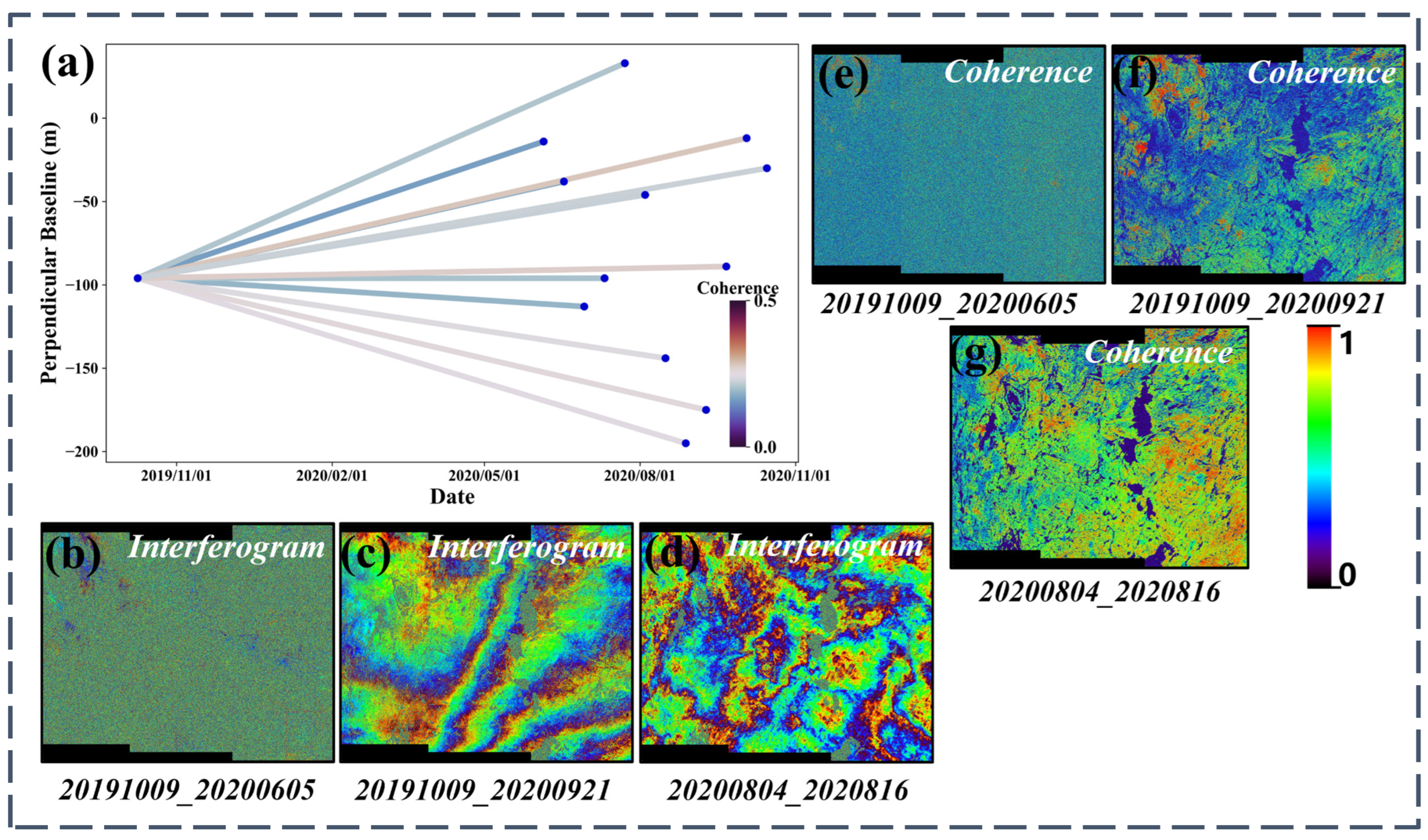
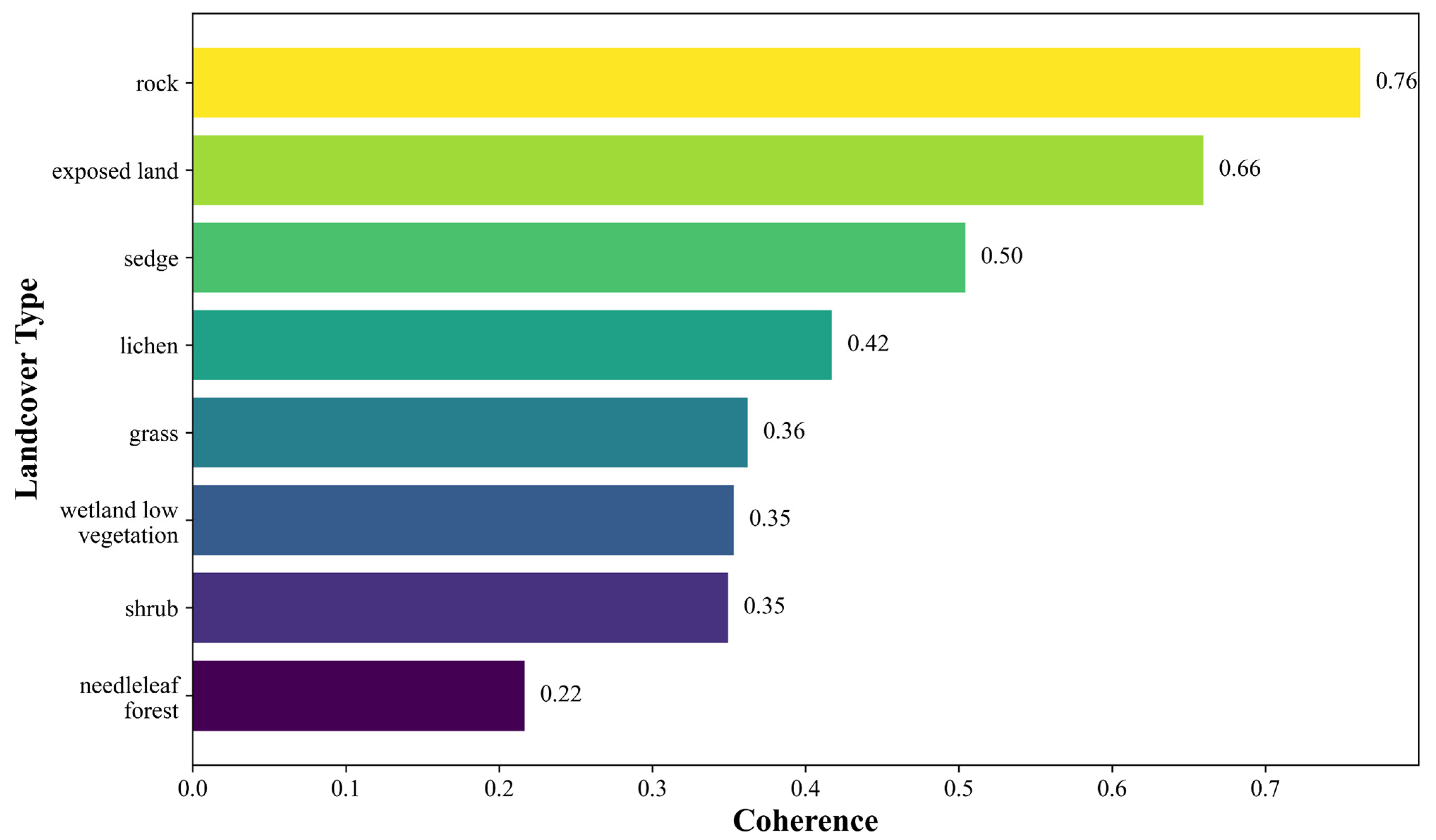
4.1. Interferometric Coherence Time Series under Different Landscape Features

Figure 4 depicts the time series of the interferometric coherence for eight typical landscape features in continuous permafrost terrain across consecutive thawing seasons: (1) rock, (2) exposed land, (3) sedge, (4) wetland low vegetation, (5) lichen, (6) grass, (7) shrub, and (8) needleleaf forest. The areas containing these landscapes were identified in the study area based on the National Land Cover Database (NLCD) land cover data for Alaska [30] and Canadian land cover data [31]. Additionally, 1 km × 1 km polygons were extracted to investigate the temporal changes in the interferometric coherence. The interferometric coherence time series depicted in Figure 4 represents the average coherence of the selected polygons. The coherence at each time point was calculated from interferogram combinations of SAR images acquired at time ti and subsequent time ti+1 in chronological order.
In general, the interferometric coherence decreases with increasing vegetation density and height due to the scattering effects of the vegetation canopy. A comparison of the average coherence of different landscape features is shown in Figure 5. Areas with rock and exposed land tend to have relatively high interferometric coherence. For other landscapes, the interferometric coherence varies, ranking from high to low as follows: sedge, lichen, grass, wetland low vegetation, dwarf shrub, and needleleaf forest. Low-lying vegetation, such as sedge, lichen, and grass, demonstrates good interferometric coherence. However, densely vegetated areas such as shrub and needleleaf forest exhibit significant decorrelation in their coherence time series due to changes in the vegetation phenology and strong variations in the dielectric properties over time and space. Low vegetation in the wetlands of North Slope of Alaska is usually located near water bodies and has high soil moisture content. This leads to lower interferometric coherence compared to sedge in other regions. The interferometric coherence time series for all the landscape features exhibit distinct seasonal characteristics. Influenced by the effects of snowmelt and permafrost freeze–thaw cycles, interferogram combinations involving SAR images acquired during the same thawing season consistently exhibit relatively high coherence. In contrast, interferogram combinations spanning the end of one thawing season and the beginning of the next season demonstrate significant decorrelation.

4.2. Long-Term Surface Deformation in Typical Permafrost Regions

4.2.1. North Slope of Alaska (sedge)

Figure 6 displays the mean deformation rate map in the LOS direction for the lowland plain of the North Slope of Alaska, covering the period from mid-June 2018 to late September 2021. This map has been generated from 343 interferograms. The mean annual deformation rate map includes long-term InSAR deformation results from DTLBs, Arctic tundra regions, and floodplains. The SAR images used were acquired over nearly the same period during four consecutive thawing seasons, generating interferogram stacks with a sufficient number of interannual connections in each frame. As a result, the seasonal deformation signals during each thawing season are largely cancelled out, enabling the derivation of the average deformation rate that represents the long-term deformation information in permafrost.
In this context, a negative velocity indicates an increase in displacement over time in the LOS direction, meaning subsidence, while a positive velocity indicates a reduction in displacement, meaning uplift.
In this study, we are interested in the surface deformation patterns in larger-scale DTLBs and tundra regions. Figure 6 shows that almost the entire lowland tundra region of the North Slope of Alaska is experiencing prolonged and gradual surface subsidence. Notably, the spatial distribution of the surface deformation patterns is closely associated with the proximity to thermokarst lakes and coastlines, indicating that the higher soil moisture content and greater heat retention in these areas substantially influence the deformation patterns compared to other regions.
Substantial subsidence is observed around several lakes (see Figure 6, Sector 2), which may correspond to the typical collapse banks observed in the evolution of thermokarst lakes [45]. Regions exhibiting substantial surface subsidence include Prudhoe Bay in the northeast and the Alaska Pipeline in the southeast. It is worth noting that Prudhoe Bay and the Alaska Pipeline are heavily impacted by human activity. The different sectors (Sector 1, Sector 2, and Sector 3) in Figure 5 highlight these key areas to demonstrate the deformation pattern in more detail.
Noticeable surface uplift patterns are observed in Utqiagvik, in the northwest corner of the North Slope, as well as in the DTLBs further from the coast. This phenomenon can be attributed to the partial drainage of thermokarst lakes, which exposes previously submerged permafrost to cold winter temperatures. Consequently, the sandy lakebed undergoes freezing expansion, resulting in surface uplift. Figure 7c,d depict optical images (sourced from Google Earth) of a thermokarst lake undergoing partial drainage in 1986 and 2020, respectively. It is evident that the edges of the lake have receded inward over time.
Seasonal displacement curves for typical uplift and subsidence areas on the Alaskan North Slope are shown in Figure 7e and Figure 8d. These graphs demonstrate the changes in the permafrost surface deformation over multiple consecutive thawing seasons. During a single thawing season, the surface deformation observed by InSAR does not always exhibit continuous subsidence, as occasional surface uplift is observed, notably coinciding with the dates of sudden temperature drops. To further support this statement, we have included additional visual data in Figure 7e and Figure 8d, marking the dates of sudden temperature drops with vertical red lines. As illustrated, the surface uplift observed by InSAR follows these temperature drops. This phenomenon can be influenced by factors such as the temperature, rainfall, and soil moisture. At Utqiagvik, 2016 GPS data revealed that a similar abnormal, temporal thaw-season heave coincided with the temporal temperature changes [46]. Furthermore, it is important to note that seasonal observations based on InSAR may not capture early thaw information. This limitation arises from the loss of interferometric coherence in wetland areas caused by processes such as snow accumulation and subsequent snowmelt. Consequently, InSAR data may not provide the absolute magnitudes for both thaw settlement and frost heave within a complete freeze–thaw cycle.
The fitted long-term mean deformation rate of the subsidence point is much lower than the average subsidence rate in a single thawing season due to frost heave during the freezing season. However, this pattern still indicates significant subsidence, pointing to considerable permafrost degradation. In contrast, the seasonal displacement pattern observed at the uplift points shows subsidence but an uplift pattern over four consecutive years of observation. During the freezing season, the permafrost surface is exposed to cold air, leading to frost heave and surface uplift. As a result, the surface elevation at the end of each thawing season is lower than at the beginning of the subsequent thawing season. If the frost heave is stronger than the thaw settlement, it can lead to long-term uplift.

4.2.2. Northern Great Bear Lake, Canada (dwarf shrub and needleleaf forest)

The mean deformation rate map for the northwestern area of Great Bear Lake is shown in Figure 9a. The observation period ranged from mid-June 2018 to early October 2021. The average coherence of this region is lower than that of the tundra region of the North Slope of Alaska. In contrast to the relatively uniform surface deformation observed in the lowland tundra region, this area exhibits significant spatial heterogeneity in the surface deformation. In particular, localized areas in the northwest and southwest directions exhibit distinct subsidence characteristics, indicating a more pronounced downward movement of the ground surface. Meanwhile, other areas in this region show a pattern similar to that observed in the North Slope, characterized by gradual surface subsidence.
Figure 9b,c show the mean deformation rate and a high-resolution optical image from the northwest region of the study area, which is a typical subsidence area affected by wildfires. Historical wildfire data for Canada were obtained through the Canadian National Fire Database (CNFDB) [47]. Two separate wildfires occurred in this region: Wildfire Area A in 2012 and Wildfire Area B in 2017. The spatial distribution of the areas affected by wildfires closely matches the distribution of severe surface subsidence observed in the mean deformation rate map. Within the wildfire-affected areas, the surface subsidence rates have increased significantly, with the highest rates up to −22.5 mm/yr. The seasonal subsidence in the fire-affected areas is particularly severe compared to the surrounding unburned areas.
For the analysis of the long-term surface deformation, we extracted all the coherent pixels within the areas affected by the two separate wildfires (2610 pixels in area A and 22,466 pixels in area B). Additionally, we selected Unburned Area C. A total of 1585 coherent pixels were extracted to provide a comparative analysis. The boxplot in Figure 10 shows the distribution of the deformation rate in three areas. The deformation results show significant surface subsidence in the two areas affected by wildfires in 2012 and 2017, respectively, indicating accelerated degradation of permafrost. The region affected by the 2012 wildfire still exhibits strong trends in surface subsidence nearly a decade later, and this subsidence is even more pronounced when compared to the 2017 wildfire. This difference in the subsidence intensity may be related to the severity and duration of both wildfire events.

4.2.3. Southern Angikuni Lake, Canada (lichen and moss)

Figure 11 displays the mean deformation rate map for the southern part of Angikuni Lake from mid-June 2018 to mid-October 2021 in the LOS direction. This area has a higher average coherence of 0.35 compared to the shrubs and sparse needleleaf forests area on the northwest side of Great Bear Lake, which has an average coherence of 0.26. Most of the region shows a mild subsidence pattern and high spatial consistency in the long-term surface deformation trends. This suggests that the permafrost in this region is experiencing a slow overall degradation process.
Compared to the lowland tundra region of the North Slope of Alaska, this region has a lower mean surface deformation rate of −3.3 mm/yr. There is a notable difference in the deformation patterns between the eastern and western sides of Hex Lake in the lower left corner of the study area. The western side, characterized by barren lichen and moss terrain, exhibits a stronger subsidence than the eastern side, which features more developed shrubland with lichen and moss (as shown in the detailed land cover raster in Figure 11c). This observation highlights the positive role of the vegetation cover type and density in mitigating long-term surface subsidence in permafrost regions.

4.3. Analysis of InSAR Results in Typical Permafrost Regions

Figure 12 shows the density distribution of the surface deformation rates in three typical permafrost regions. Most permafrost areas in typical North American circum-Arctic landscapes have surface deformation rates between −15 mm/yr and 10 mm/yr. We assume that areas with deformation rates greater than −5 mm/yr are considered to be experiencing permafrost degradation, based on the findings from [48]. In our study area, permafrost degradation occurs in 32.3% of the North slope of Alaska (sedge-dominated tundra), 47.3% of the Northern Great Bear Lake (dwarf shrub and needleleaf forest), and 33.0% of the Southern Angikuni Lake (lichen and moss). Overall, more than one-third of the North American circum-Arctic permafrost region in the study area is experiencing permafrost degradation.
As shown in Figure 12, the Northern Great Bear Lake has the highest percentage of permafrost degradation. There are areas of severe subsidence in the region, with deformation rates greater than −25 mm/yr, which can be attributed to the severe impact of wildfires on permafrost degradation. The subsidence rates in the degraded permafrost of the Southern Angikuni Lake are concentrated in the range of −10 mm/yr to −5 mm/yr, showing mild subsidence compared to the degraded areas in the other two regions. The proportion of degraded permafrost on the North Slope of Alaska is similar to that of the Southern Angikuni Lake, but the density distribution of the subsidence rates is more dispersed. This is primarily due to the substantial uplift observed in some areas of Alaska, where frost heave is often stronger than thaw settlement, leading to long-term uplift and positive deformation rates. In addition, the study area on the North Slope of Alaska is much larger than the Southern Angikuni Lake, which makes the spatial variability of the InSAR results more pronounced. Therefore, the proportion of positive values in the density distribution of the deformation rates is highest in this region.

5. Discussion

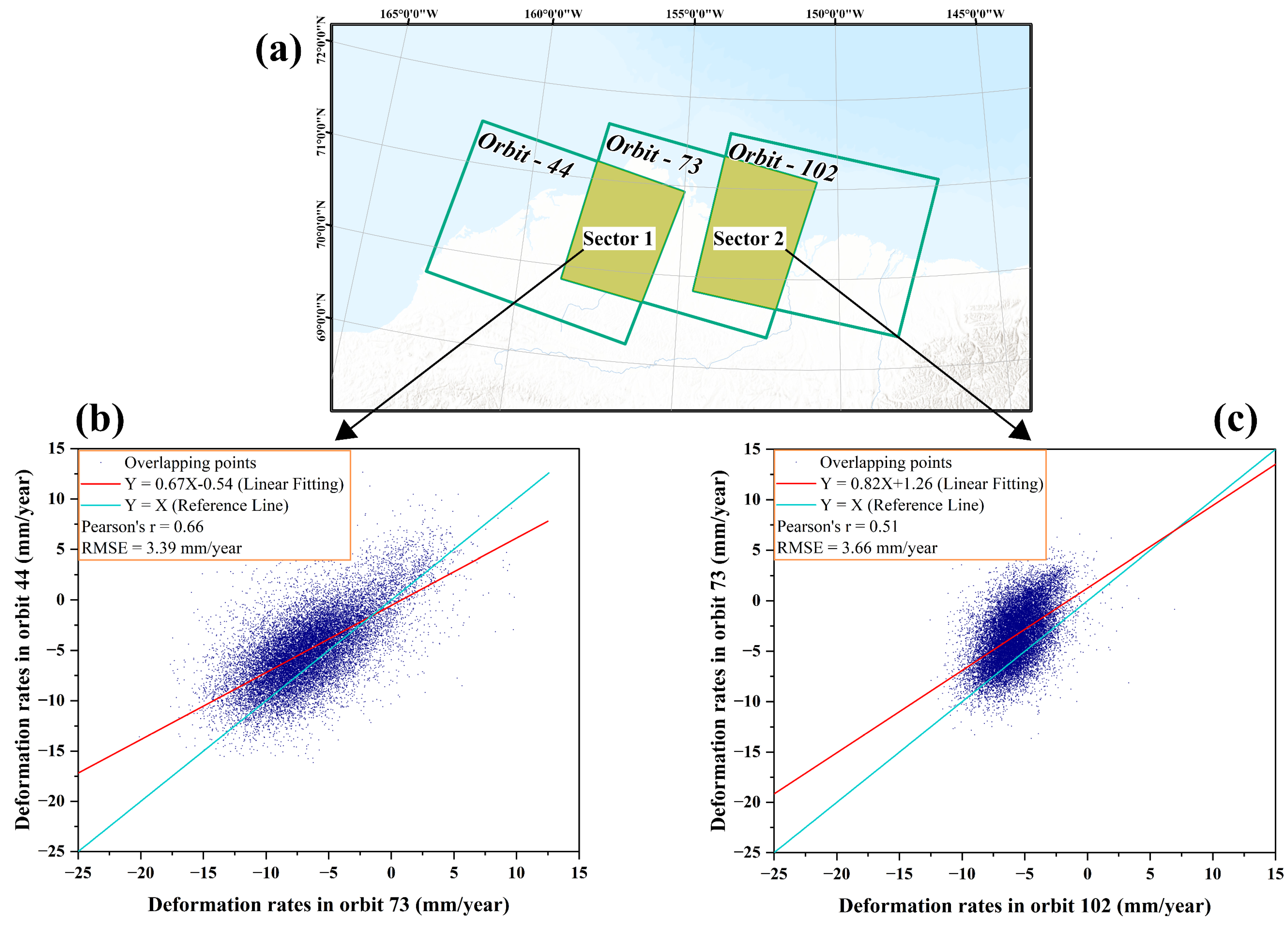
5.1. Precision Validation of the InSAR Technique

In most North American circum-Arctic permafrost regions, measuring surface deformation in the field is difficult due to their remote and harsh environment Therefore, we adopted the deformation result verification method outlined in reference [18]. We calculated and analyzed Pearson’s correlation coefficient (Pearson’s r) for the mean annual deformation rates in overlapping regions and the root mean square error (RMSE) to assess the precision of InSAR technique.
As shown in Figure 13, 20,000 random points were selected within the overlapping regions of orbit 44 and orbit 73 (Sector 1), as well as orbit 73 and orbit 102 (Sector 2), to compute Pearson’s r and the RMSE. The Pearson’s r values for Sector 1 and Sector 2 were found to be 0.66 and 0.51, indicating a significant linear relationship between deformation results in overlapping regions. The RMSE of 3.39 mm/yr for Sector 1 and 3.66 mm/yr for Sector 2 suggest an acceptable level of deviation between the average deformation rates calculated from all the co-registered images, particularly when considering the overall range of deformation rates. The Pearson’s r and RMSE results demonstrate the consistency and precision of the deformation results obtained by InSAR in overlapping regions.
However, these metrics do not confirm the absolute accuracy of the measurements. Given the harsh environment and lack of field measurements in the North Slope of Alaska, Pearson’s r and the RMSE provide a useful, albeit indirect, means of validating the InSAR results. In addition, in the study area of Northern Great Bear Lake, the InSAR results show significant local subsidence characteristics, and the distribution range of local subsidence matches very well with the wildfire range provided by the CNFDB, which can also indirectly prove the correctness of the InSAR results (see Figure 9).

5.2. In Situ Comparison

We used the average annual site end-of-season thaw depth, obtained from the Circumpolar Active Layer Monitoring (CALM) program established by the International Permafrost Association [49], to further validate the reliability of InSAR technology in measuring seasonal subsidence and long-term permafrost settlement patterns. The soil thaw was measured by inserting a metal probe into the soil to the point of resistance, and it can represent the ALT. Ref. [50] used a scatter plot depicting the mean InSAR displacement against the ALT within a region and calculated the R2 to validate a significant linear correlation between regions with a greater ALT and larger displacements.
There are two CALM sites (U1 and U2) 600 m apart in Utqiagvik, northwest of Alaska North Slope (Figure 6 Sector 1). These two sites are unique within the study area as they consistently provided data from 2018 to 2021, employing spatially oriented mechanical probing at fixed intervals on a grid. The annual ALT for the region is determined by calculating the mean thaw depth for each thawing season at both sites. For the mean InSAR displacement in each thawing season, we selected a 2 km × 2 km polygon that included both sites and differenced the deformation between the end and beginning of each thawing season, followed by taking the mean. Table 2 and Table 3 provide detailed information on this.
Figure 14 shows the relationship between the ALT and mean displacement for each thawing season, with the calculated Pearson’s r and R2 values of 0.91 and 0.84, demonstrating a significant linear correlation between them. From 2018 to 2021, both the ALT and mean displacement show a common trend of initially increasing and then decreasing. Both the highest mean displacement and the highest recorded thaw depth occurred in 2019, followed by a subsequent decline.

5.3. Effectiveness of Sentinel-1 InSAR over Continuous Permafrost

The shorter revisit period of the Sentinel-1 satellite has led to favorable results in the application of InSAR technology for long-term deformation monitoring of Arctic permafrost. The interferogram stack used did not show significant decorrelation within a single thawing season or between adjacent thawing seasons, maintaining consistency over individual seasons and even consecutive years. Previous research in the Prudhoe Bay region of the Alaska North Slope has shown that deformation differences attributed to atmospheric delays never exceed 1 mm under any circumstances, with atmospheric errors considerably smaller than the systematic errors associated with InSAR technology [10]. The temporal low correlation of atmospheric artifacts, combined with a sufficient number of high-quality interferograms spanning four consecutive years in our interferogram stack, further mitigates the impact of atmospheric errors. The consistency of the results in overlapping regions between different frames on the Alaska North Slope further validates the reliability of the Sentinel-1 InSAR results.
After long-term deformation monitoring of three typical permafrost landscapes, we concluded that permafrost in the North American circum-Arctic region is undergoing degradation, which is externally manifested by widespread and persistent surface subsidence. However, different landscape types showed substantial variations in the magnitude of these changes, likely influenced by factors such as the vegetation dielectric constant, canopy volume scattering, soil moisture, and others. The temporal variability of these influencing factors at the local spatial scale could contribute to the observed spatial variability in the InSAR observations. Additionally, in needleleaf forests and shrub areas, C-band radar signals have difficulty penetrating the dense vegetation canopies, further reducing the interferometric coherence levels. Therefore, a detailed comparison with the L-band InSAR observations is necessary to validate the observation accuracy of Sentinel-1 in these areas and to assess the deformation differences compared to long-wave results in future research.
Seasonal thawing subsidence is mainly caused by thawing of the active layer and permafrost table, while frost heave is the process by which water turns into ice during the freezing season, resulting in an increase in volume. Generally, the subsidence and uplift magnitudes caused by the active layer during each freeze–thaw cycle are similar. Therefore, it is generally assumed that the long-term surface subsidence observed by InSAR is mainly driven by thawing of the underlying ice-rich permafrost table, indicating permafrost degradation. Most of the seasonal subsidence or uplift caused by ALT changes is offset by continuous observations over a multi-year period. These observations enable the extraction of long-term deformation trends from seasonal subsidence and their use as a representation of permafrost table degradation. However, this also introduces greater uncertainty in the long-term deformation rate of the final fit.
The slight uplift observed in localized areas near thermokarst lakes can be attributed to lake dynamics closely related to lowland permafrost evolution. Lake drainage processes expose the fresh permafrost surface to the cold air, which promotes permafrost aggradation, and increase the likelihood of future degradation [34,45,51].

6. Conclusions

In this study, the time series surface deformation of permafrost was analyzed from 2018 to 2021 by using Sentinel-1 SAR data from typical permafrost landscapes in North America. To address the temporal decorrelation caused by prolonged snow cover on polar permafrost, we proposed a two-stage interferogram selection strategy and obtained effective surface deformation results. Our research results reveal the permafrost degradation under different regions with varying land covers. The main conclusions of our study are as follows:
  • Two-stage interferogram selection strategy: Winter snow cover leads to decorrelation, limiting our data acquisition to the summer months. After analyzing all the possible interferograms for two adjacent thawing seasons, we found that the interannual interferograms for approximate thawing days in adjacent years showed sufficiently high coherence. This suggests that it is possible to reconstruct the long-term deformation time series of permafrost. Therefore, we introduce a two-stage interferogram selection strategy that enables us to infer the effective multi-year deformation of permafrost, thereby reflecting its degradation status.
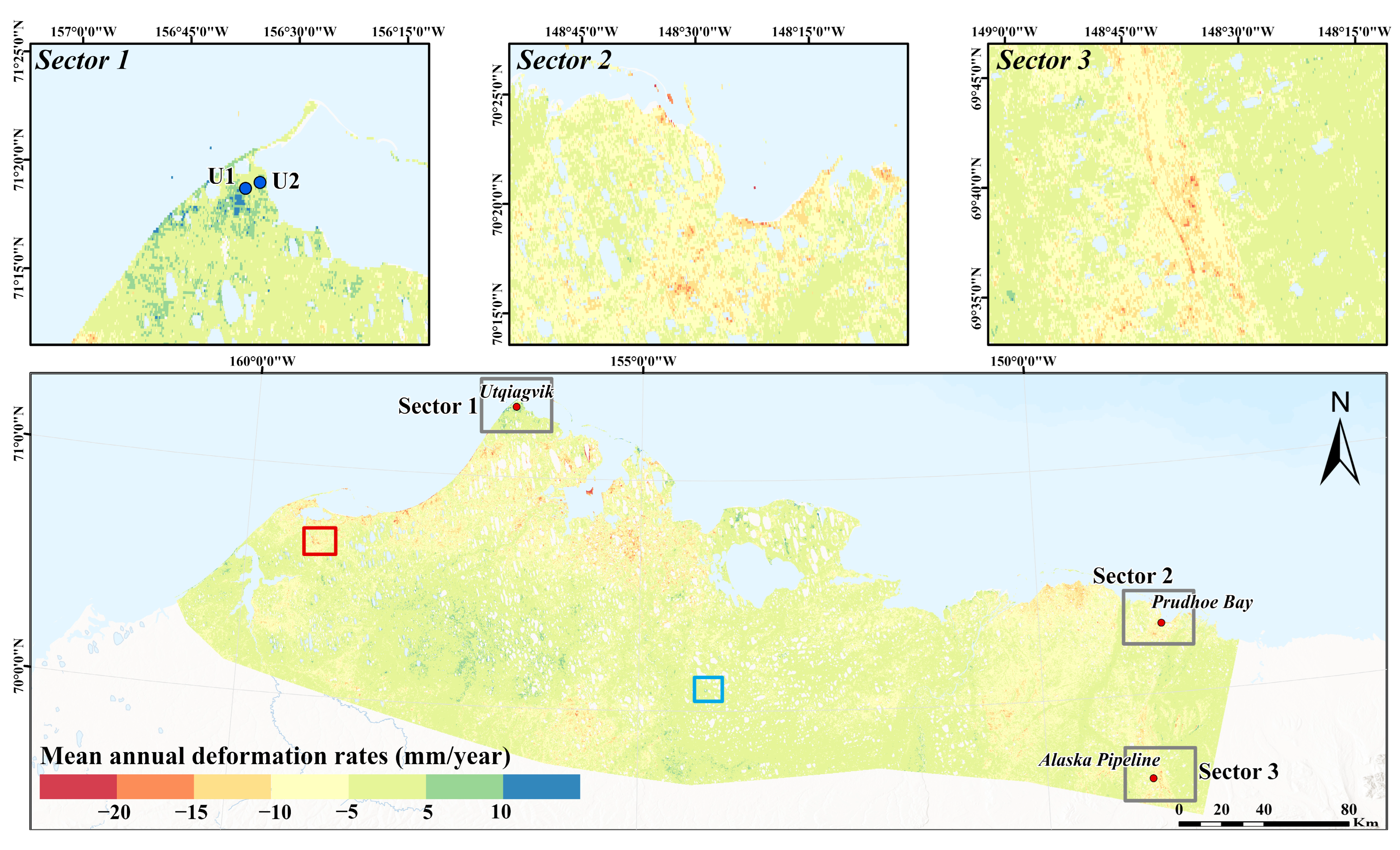
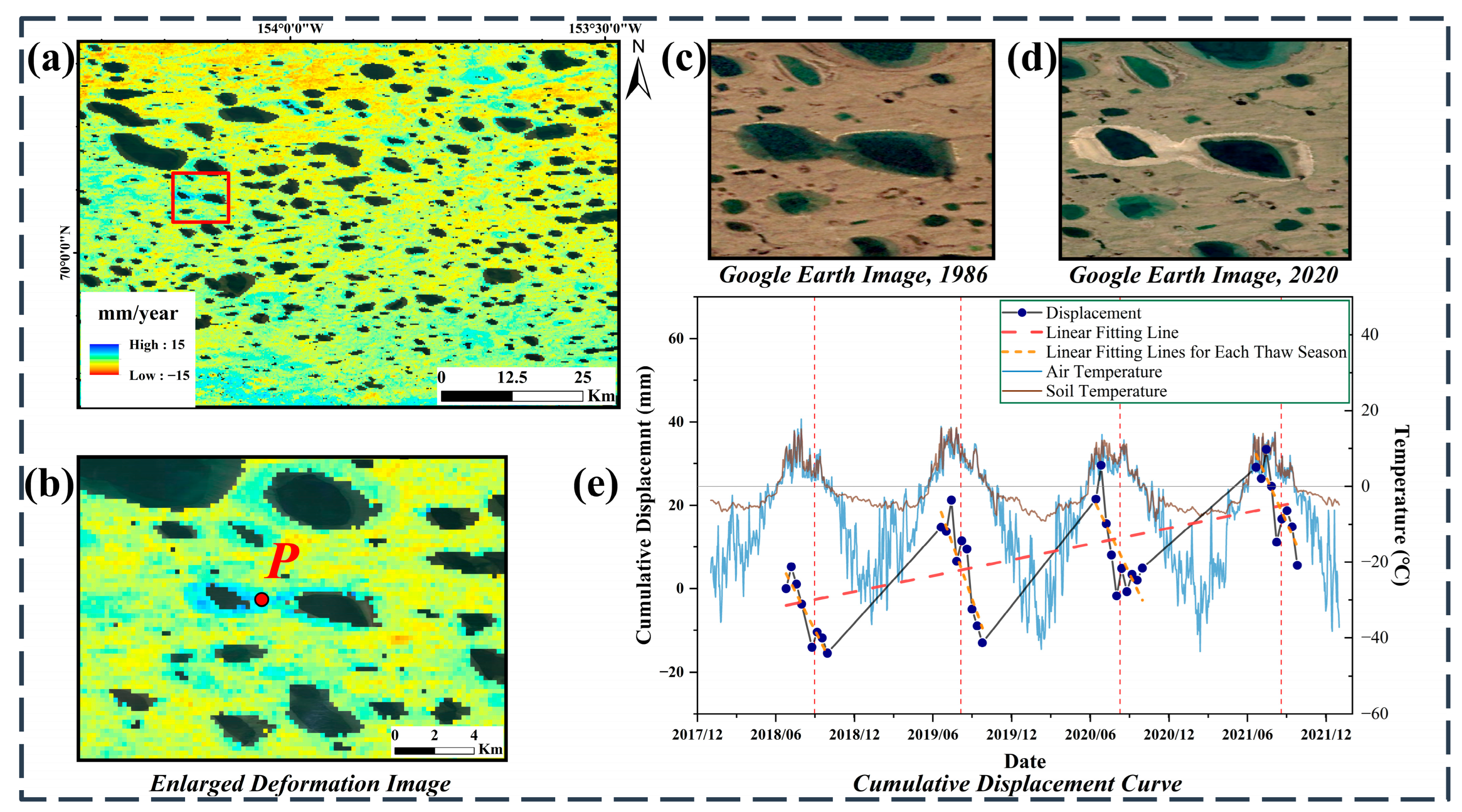
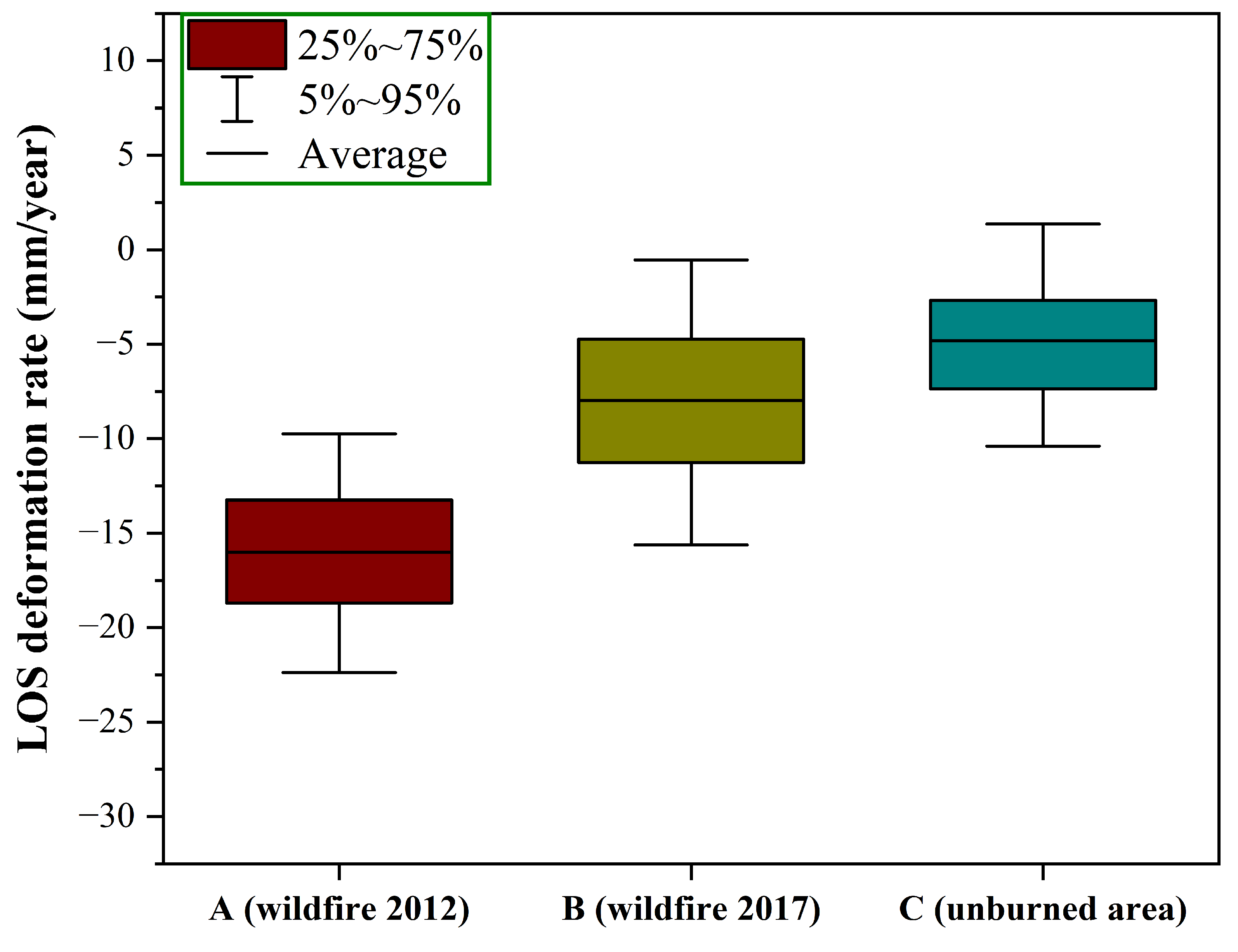
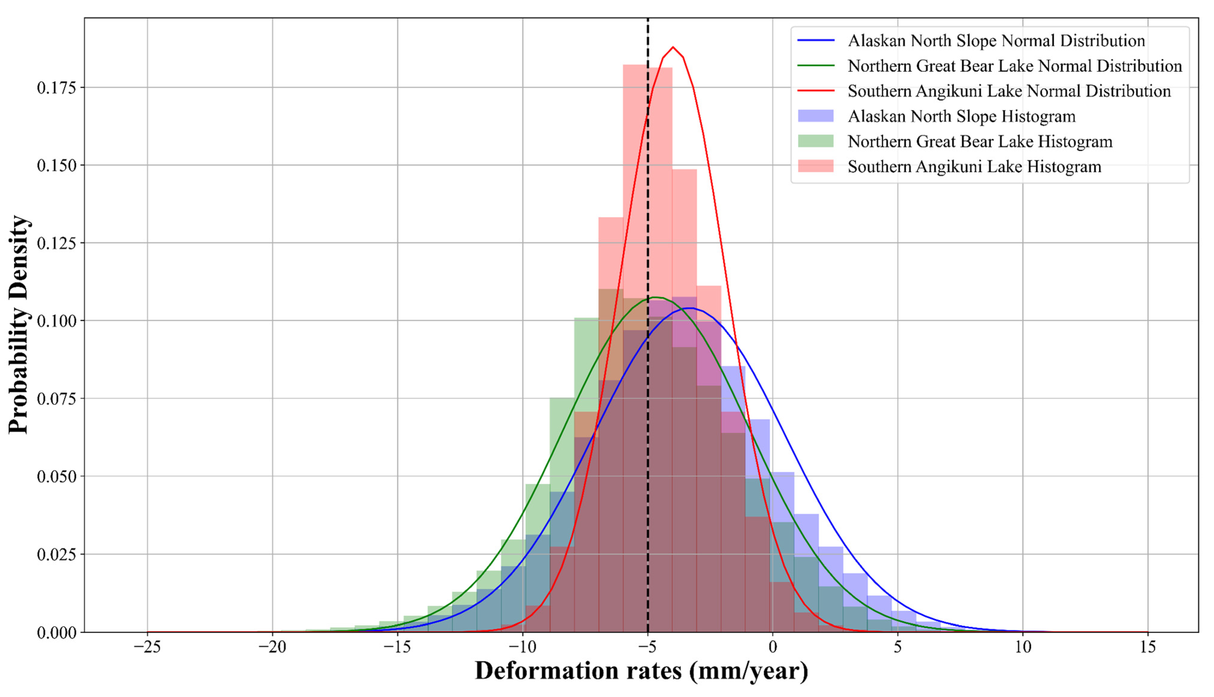
  • Deformation patterns in North America: (1) Most permafrost areas in typical North American circum-Arctic landscapes have deformation rates between −15 mm/yr and 10 mm/yr. Using −5 mm/yr as the threshold, permafrost degradation occurs in 32.3% of the sedge-dominated tundra region, 47.3% of the dwarf shrub and needleleaf forest region, and 33.0% of the lichen and moss region. (2) In the shrub and needleleaf forest areas affected by wildfires, there is a trend of accelerated surface subsidence, with subsidence rates ranging from −25 mm/yr to −15 mm/yr. Even a decade after the wildfires, severe subsidence is still present in these areas, reflecting the long-term and profound effects of wildfires on permafrost. (3) Other areas of severe permafrost subsidence are concentrated in the coastal alluvial plains of the Alaskan North Slope and inland lakeshore plains, which may be due to the erosive impacts of seawater or lake water that intensifies the permafrost degradation. (4) Notably, the drained thermokarst lake basin on the Alaskan North Slope exhibits significant surface uplift. This is attributed to the partial drainage of thermokarst lakes, which exposes previously submerged permafrost to low winter temperatures, resulting in greater frost-heave uplift. This suggests that areas where uplift is occurring may also be experiencing degradation of permafrost.
  • Degradation of permafrost in North America: The surface deformation patterns of permafrost in the North American circum-Arctic, as obtained through multi-year InSAR monitoring, indicate that more than one-third of the permafrost in North America in the study area is experiencing degradation. Permafrost degradation is more severe in areas affected by wildfires and human activities. Such degradation can lead to the release of large amounts of carbon stored in permafrost, thereby accelerating global warming.

Supplementary Materials

The following supporting information can be downloaded at https://www.mdpi.com/article/10.3390/rs16152809/s1, Figure S1: interferogram_44–357; Figure S2: interferogram_73–356; Figure S3: interferogram_102–356; Figure S4: interferogram_165–199; Figure S5: interferogram_166–217.

Author Contributions

Conceptualization, S.G., C.W. and Y.T.; formal analysis, S.G.; methodology, S.G. and C.W.; software, S.G., Y.T., L.Z. and P.Y.; validation, S.G. and C.W.; writing—original draft preparation, S.G.; writing—review and editing, C.W., L.Z. and H.Z.; visualization, S.G. and T.L.; supervision, C.W.; project administration, C.W.; funding acquisition, C.W. All authors have read and agreed to the published version of the manuscript.

Funding

This paper was funded by the National Natural Science Foundation of China (NSFC), Grant No. 41930110 and Grant No. 42327801.

Data Availability Statement

The data that support the findings of this study are available from the corresponding author upon reasonable request.

Acknowledgments

The authors would like to thank the European Space Agency (ESA) for the Sentinel-1 data and the Circumpolar Active Layer Monitoring (CALM) program for the active layer thickness (ALT) data.

Conflicts of Interest

The authors declare no conflicts of interest.

References

  1. Turetsky, M.R.; Abbott, B.W.; Jones, M.C.; Walter Anthony, K.; Olefeldt, D.; Schuur, E.A.G.; Koven, C.; McGuire, A.D.; Grosse, G.; Kuhry, P.; et al. Permafrost Collapse Is Accelerating Carbon Release. Nature 2019, 569, 32–34. [Google Scholar] [CrossRef]
  2. Jones, B.M.; Grosse, G.; Farquharson, L.M.; Roy-Léveillée, P.; Veremeeva, A.; Kanevskiy, M.Z.; Gaglioti, B.V.; Breen, A.L.; Parsekian, A.D.; Ulrich, M.; et al. Lake and Drained Lake Basin Systems in Lowland Permafrost Regions. Nat. Rev. Earth Environ. 2022, 3, 85–98. [Google Scholar] [CrossRef]
  3. Pörtner, H.-O.; Roberts, D.C.; Masson-Delmotte, V.; Zhai, P.; Tignor, M.; Poloczanska, E.; Weyer, N. The Ocean and Cryosphere in a Changing Climate. IPCC Spec. Rep. Ocean Cryosphere A Chang. Clim. 2019, 1155, 203–321. [Google Scholar]
  4. Biskaborn, B.K.; Smith, S.L.; Noetzli, J.; Matthes, H.; Vieira, G.; Streletskiy, D.A.; Schoeneich, P.; Romanovsky, V.E.; Lewkowicz, A.G.; Abramov, A.; et al. Permafrost Is Warming at a Global Scale. Nat. Commun. 2019, 10, 264. [Google Scholar] [CrossRef]
  5. Anthony, K.M.W.; Zimov, S.A.; Grosse, G.; Jones, M.C.; Anthony, P.M.; Iii, F.S.C.; Finlay, J.C.; Mack, M.C.; Davydov, S.; Frenzel, P.; et al. A Shift of Thermokarst Lakes from Carbon Sources to Sinks during the Holocene Epoch. Nature 2014, 511, 452–456. [Google Scholar] [CrossRef]
  6. Hugelius, G.; Loisel, J.; Chadburn, S.; Jackson, R.B.; Jones, M.; MacDonald, G.; Marushchak, M.; Olefeldt, D.; Packalen, M.; Siewert, M.B.; et al. Large Stocks of Peatland Carbon and Nitrogen Are Vulnerable to Permafrost Thaw. Proc. Natl. Acad. Sci. USA 2020, 117, 20438–20446. [Google Scholar] [CrossRef]
  7. Miner, K.R.; Turetsky, M.R.; Malina, E.; Bartsch, A.; Tamminen, J.; McGuire, A.D.; Fix, A.; Sweeney, C.; Elder, C.D.; Miller, C.E. Permafrost Carbon Emissions in a Changing Arctic. Nat. Rev. Earth Environ. 2022, 3, 55–67. [Google Scholar] [CrossRef]
  8. Schuur, E.A.G.; McGuire, A.D.; Schädel, C.; Grosse, G.; Harden, J.W.; Hayes, D.J.; Hugelius, G.; Koven, C.D.; Kuhry, P.; Lawrence, D.M.; et al. Climate Change and the Permafrost Carbon Feedback. Nature 2015, 520, 171–179. [Google Scholar] [CrossRef]
  9. Voigt, C.; Marushchak, M.E.; Abbott, B.W.; Biasi, C.; Elberling, B.; Siciliano, S.D.; Sonnentag, O.; Stewart, K.J.; Yang, Y.; Martikainen, P.J. Nitrous Oxide Emissions from Permafrost-Affected Soils. Nat. Rev. Earth Environ. 2020, 1, 420–434. [Google Scholar] [CrossRef]
  10. Liu, L.; Zhang, T.; Wahr, J. InSAR Measurements of Surface Deformation over Permafrost on the North Slope of Alaska. J. Geophys. Res. Earth Surf. 2010, 115, F03023. [Google Scholar] [CrossRef]
  11. Streletskiy, D.A.; Shiklomanov, N.I.; Little, J.D.; Nelson, F.E.; Brown, J.; Nyland, K.E.; Klene, A.E. Thaw Subsidence in Undisturbed Tundra Landscapes, Barrow, Alaska, 1962–2015. Permafr. Periglac 2017, 28, 566–572. [Google Scholar] [CrossRef]
  12. Zhao, R.; Li, Z.; Feng, G.; Wang, Q.; Hu, J. Monitoring Surface Deformation over Permafrost with an Improved SBAS-InSAR Algorithm: With Emphasis on Climatic Factors Modeling. Remote Sens. Environ. 2016, 184, 276–287. [Google Scholar] [CrossRef]
  13. Rouyet, L.; Lauknes, T.R.; Christiansen, H.H.; Strand, S.M.; Larsen, Y. Seasonal Dynamics of a Permafrost Landscape, Adventdalen, Svalbard, Investigated by InSAR. Remote Sens. Environ. 2019, 231, 111236. [Google Scholar] [CrossRef]
  14. Zhang, Z.; Lin, H.; Wang, M.; Liu, X.; Chen, Q.; Wang, C.; Zhang, H. A Review of Satellite Synthetic Aperture Radar Interferometry Applications in Permafrost Regions: Current Status, Challenges, and Trends. IEEE Geosci. Remote Sens. Mag. 2022, 10, 93–114. [Google Scholar] [CrossRef]
  15. Ma, P.; Wang, W.; Zhang, B.; Wang, J.; Shi, G.; Huang, G.; Chen, F.; Jiang, L.; Lin, H. Remotely Sensing Large- and Small-Scale Ground Subsidence: A Case Study of the Guangdong–Hong Kong–Macao Greater Bay Area of China. Remote Sens. Environ. 2019, 232, 111282. [Google Scholar] [CrossRef]
  16. Wang, C.; Tang, Y.; Zhang, H.; You, H.; Zhang, W.; Duan, W.; Wang, J.; Dong, L.; Zhang, B. First Mapping of China Surface Movement Using Supercomputing Interferometric SAR Technique. Sci. Bull. 2021, 66, 1608–1610. [Google Scholar] [CrossRef] [PubMed]
  17. Zou, L.; Wang, C.; Tang, Y.; Zhang, B.; Zhang, H.; Dong, L. Interferometric SAR Observation of Permafrost Status in the Northern Qinghai-Tibet Plateau by ALOS, ALOS-2 and Sentinel-1 between 2007 and 2021. Remote Sens. 2022, 14, 1870. [Google Scholar] [CrossRef]
  18. Zheng, X.; Wang, C.; Tang, Y.; Zhang, H.; Li, T.; Zou, L.; Guan, S. Adaptive High Coherence Temporal Subsets SBAS-InSAR in Tropical Peatlands Degradation Monitoring. Remote Sens. 2023, 15, 4461. [Google Scholar] [CrossRef]
  19. Liu, L.; Schaefer, K.; Gusmeroli, A.; Grosse, G.; Jones, B.M.; Zhang, T.; Parsekian, A.D.; Zebker, H.A. Seasonal Thaw Settlement at Drained Thermokarst Lake Basins, Arctic Alaska. Cryosphere 2014, 8, 815–826. [Google Scholar] [CrossRef]
  20. Liu, L.; Jafarov, E.E.; Schaefer, K.M.; Jones, B.M.; Zebker, H.A.; Williams, C.A.; Rogan, J.; Zhang, T. InSAR Detects Increase in Surface Subsidence Caused by an Arctic Tundra Fire. Geophys. Res. Lett. 2014, 41, 3906–3913. [Google Scholar] [CrossRef]
  21. Strozzi, T.; Antonova, S.; Günther, F.; Mätzler, E.; Vieira, G.; Wegmüller, U.; Westermann, S.; Bartsch, A. Sentinel-1 SAR Interferometry for Surface Deformation Monitoring in Low-Land Permafrost Areas. Remote Sens. 2018, 10, 1360. [Google Scholar] [CrossRef]
  22. Short, N.; LeBlanc, A.-M.; Sladen, W.; Oldenborger, G.; Mathon-Dufour, V.; Brisco, B. RADARSAT-2 D-InSAR for Ground Displacement in Permafrost Terrain, Validation from Iqaluit Airport, Baffin Island, Canada. Remote Sens. Environ. 2014, 141, 40–51. [Google Scholar] [CrossRef]
  23. Wang, L.; Marzahn, P.; Bernier, M.; Ludwig, R. Sentinel-1 InSAR Measurements of Deformation over Discontinuous Permafrost Terrain, Northern Quebec, Canada. Remote Sens. Environ. 2020, 248, 111965. [Google Scholar] [CrossRef]
  24. Zebker, H.A.; Rosen, P.A.; Hensley, S. Atmospheric Effects in Interferometric Synthetic Aperture Radar Surface Deformation and Topographic Maps. J. Geophys. Res. Solid Earth 1997, 102, 7547–7563. [Google Scholar] [CrossRef]
  25. Wang, L.; Marzahn, P.; Bernier, M.; Jacome, A.; Poulin, J.; Ludwig, R. Comparison of TerraSAR-X and ALOS PALSAR Differential Interferometry with Multisource DEMs for Monitoring Ground Displacement in a Discontinuous Permafrost Region. IEEE J.-Stars 2017, 10, 4074–4093. [Google Scholar] [CrossRef]
  26. Berardino, P.; Fornaro, G.; Lanari, R.; Sansosti, E. A New Algorithm for Surface Deformation Monitoring Based on Small Baseline Differential SAR Interferograms. IEEE Trans. Geosci. Remote 2002, 40, 2375–2383. [Google Scholar] [CrossRef]
  27. Chen, F.; Lin, H.; Li, Z.; Chen, Q.; Zhou, J. Interaction between Permafrost and Infrastructure along the Qinghai–Tibet Railway Detected via Jointly Analysis of C- and L-Band Small Baseline SAR Interferometry. Remote Sens. Environ. 2012, 123, 532–540. [Google Scholar] [CrossRef]
  28. Hooper, A. A Multi-Temporal InSAR Method Incorporating Both Persistent Scatterer and Small Baseline Approaches. Geophys. Res. Lett. 2008, 35, 532–540. [Google Scholar] [CrossRef]
  29. Obu, J.; Westermann, S.; Bartsch, A.; Berdnikov, N.; Christiansen, H.H.; Dashtseren, A.; Delaloye, R.; Elberling, B.; Etzelmüller, B.; Kholodov, A.; et al. Northern Hemisphere Permafrost Map Based on TTOP Modelling for 2000–2016 at 1 km2 Scale. Earth-Sci. Rev. 2019, 193, 299–316. [Google Scholar] [CrossRef]
  30. Wickham, J.; Stehman, S.V.; Sorenson, D.G.; Gass, L.; Dewitz, J.A. Thematic Accuracy Assessment of the NLCD 2016 Land Cover for the Conterminous United States. Remote Sens. Environ. 2021, 257, 112357. [Google Scholar] [CrossRef]
  31. Latifovic, R.; Pouliot, D.; Olthof, I. Circa 2010 Land Cover of Canada: Local Optimization Methodology and Product Development. Remote Sens. 2017, 9, 1098. [Google Scholar] [CrossRef]
  32. Brown, J.; Sellmann, P.V. Permafrost and Coastal Plain History of Arctic Alaska. Alsk. Arct. Tundra. Tech. Pap. 1973, 25, 31–47. [Google Scholar]
  33. Survey (US), G.; Reimnitz, E.; Graves, S.M.; Barnes, P.W. Beaufort Sea Coastal Erosion, Sediment Flux, Shoreline Evolution, and the Erosional Shelf Profile; US Geological Survey: Reston, VA, USA, 1988.
  34. Jones, B.M.; Arp, C.D. Observing a Catastrophic Thermokarst Lake Drainage in Northern Alaska. Permafr. Periglac 2015, 26, 119–128. [Google Scholar] [CrossRef]
  35. Olefeldt, D.; Goswami, S.; Grosse, G.; Hayes, D.; Hugelius, G.; Kuhry, P.; McGuire, A.D.; Romanovsky, V.E.; Sannel, A.B.K.; Schuur, E.A.G.; et al. Circumpolar Distribution and Carbon Storage of Thermokarst Landscapes. Nat. Commun. 2016, 7, 13043. [Google Scholar] [CrossRef]
  36. Liu, L.; Schaefer, K.M.; Chen, A.C.; Gusmeroli, A.; Zebker, H.A.; Zhang, T. Remote Sensing Measurements of Thermokarst Subsidence Using InSAR. J. Geophys. Res. Earth Surf. 2015, 120, 1935–1948. [Google Scholar] [CrossRef]
  37. Bartsch, A.; Leibman, M.; Strozzi, T.; Khomutov, A.; Widhalm, B.; Babkina, E.; Mullanurov, D.; Ermokhina, K.; Kroisleitner, C.; Bergstedt, H. Seasonal Progression of Ground Displacement Identified with Satellite Radar Interferometry and the Impact of Unusually Warm Conditions on Permafrost at the Yamal Peninsula in 2016. Remote Sens. 2019, 11, 1865. [Google Scholar] [CrossRef]
  38. Zebker, H.A.; Villasenor, J. Decorrelation in Interferometric Radar Echoes. IEEE Trans. Geosci. Remote Sens. 1992, 30, 950–959. [Google Scholar] [CrossRef]
  39. Costantini, M. A Novel Phase Unwrapping Method Based on Network Programming. IEEE Trans. Geosci. Remote Sens. 1998, 36, 813–821. [Google Scholar] [CrossRef]
  40. Chen, C.W.; Zebker, H.A. Phase Unwrapping for Large SAR Interferograms: Statistical Segmentation and Generalized Network Models. IEEE Trans. Geosci. Remote Sens. 2002, 40, 1709–1719. [Google Scholar] [CrossRef]
  41. Pullman, E.R.; Torre Jorgenson, M.; Shur, Y. Thaw Settlement in Soils of the Arctic Coastal Plain, Alaska. Arct. Antarct. Alp. Res. 2007, 39, 468–476. [Google Scholar] [CrossRef]
  42. Doin, M.-P.; Lasserre, C.; Peltzer, G.; Cavalié, O.; Doubre, C. Corrections of Stratified Tropospheric Delays in SAR Interferometry: Validation with Global Atmospheric Models. J. Appl. Geophys. 2009, 69, 35–50. [Google Scholar] [CrossRef]
  43. Rudy, A.C.A.; Lamoureux, S.F.; Treitz, P.; Short, N.; Brisco, B. Seasonal and Multi-Year Surface Displacements Measured by DInSAR in a High Arctic Permafrost Environment. Int. J. Appl. Earth Obs. 2018, 64, 51–61. [Google Scholar] [CrossRef]
  44. Usai, S. A Least Squares Database Approach for SAR Interferometric Data. IEEE Trans. Geosci. Remote Sens. 2003, 41, 753–760. [Google Scholar] [CrossRef]
  45. Grosse, G.; Jones, B.M.; Arp, C.D. Thermokarst Lakes, Drainage, and Drained Basins. In Treatise on Geomorphology; Shroder, J.F., Ed.; Elsevier: Amsterdam, The Netherlands, 2013; Volume 8, pp. 325–353. [Google Scholar]
  46. Hu, Y.; Liu, L.; Larson, K.M.; Schaefer, K.M.; Zhang, J.; Yao, Y. GPS Interferometric Reflectometry Reveals Cyclic Elevation Changes in Thaw and Freezing Seasons in a Permafrost Area (Barrow, Alaska). Geophys. Res. Lett. 2018, 45, 5581–5589. [Google Scholar] [CrossRef]
  47. Fraser, R.H.; Li, Z.; Cihlar, J. Hotspot and NDVI Differencing Synergy (HANDS): A New Technique for Burned Area Mapping over Boreal Forest. Remote Sens. Environ. 2000, 74, 362–376. [Google Scholar] [CrossRef]
  48. Deng, H.; Zhang, Z.; Wu, Y. Accelerated Permafrost Degradation in Thermokarst Landforms in Qilian Mountains from 2007 to 2020 Observed by SBAS-InSAR. Ecol. Indic. 2024, 159, 111724. [Google Scholar] [CrossRef]
  49. Brown, J.; Hinkel, K.M.; Nelson, F. The Circumpolar Active Layer Monitoring (CALM) Program: Research Designs and Initial Results. Polar Geogr. 2000, 24, 166–258. [Google Scholar] [CrossRef]
  50. Jung, Y.T.; Park, S.-E.; Kim, H.-C. Observation of Spatial and Temporal Patterns of Seasonal Ground Deformation in Central Yakutia Using Time Series InSAR Data in the Freezing Season. Remote Sens. Environ. 2023, 293, 113615. [Google Scholar] [CrossRef]
  51. Chen, Y.; Liu, A.; Cheng, X. Detection of Thermokarst Lake Drainage Events in the Northern Alaska Permafrost Region. Sci. Total Environ. 2022, 807, 150828. [Google Scholar] [CrossRef]
Figure 1. (a) The coverage of Sentinel-1 images in the study areas, where the background permafrost zonation is from [29]. (b) The land cover in the study areas, where detailed labeling information can be found in [30] for Alaska and [31] for Canada.
Remotesensing 16 02809 g001
Figure 2. Flowchart of InSAR processing.
Remotesensing 16 02809 g002
Figure 3. Examples of interferograms and interferometric coherence maps in end-to-begin and end-to-end. (a) Mean interferometric coherence. (b,e) Interferogram and coherence map in end-to-begin. (c,f) Interferogram and coherence map in end-to-end. (d,g) Interferogram and coherence map within a single thawing season.
Remotesensing 16 02809 g003
Figure 4. Coherence over the consecutive four thawing seasons. The blue lines represent the coherence calculated from the interferogram combinations of SAR images acquired at time ti and ti+1 in chronological order.
Remotesensing 16 02809 g004
Figure 5. Average interferometric coherence of different landscape features.
Remotesensing 16 02809 g005
Figure 6. Mean annual deformation rates of the North Slope of Alaska from mid-June 2018 to the end of September 2021. Sector 1 shows an enlarged view of Utqiagvik (U1 and U2 representing specific active layer monitoring sites); Sector 2 shows an enlarged view of Prudhoe Bay; Sector 3 shows an enlarged view along the alignment of the Alaska Pipeline. The blue and red boxes are the uplift area in Figure 7 and the subsidence area in Figure 8, respectively.
Remotesensing 16 02809 g006
Figure 7. Deformation results and displacement curves in a typical uplift area. (a) Mean annual deformation rates. (b) Enlarged deformation image of the typical uplift area. (c,d) Optical images of the typical uplift area in 1986 and 2020 (sourced from Google Earth). (e) Cumulative displacement curve at point P (154.155°W, 70.092°N), air and soil temperature data sourced from the ECMWF Reanalysis v5 (ERA5-Land) dataset.
Remotesensing 16 02809 g007
Figure 8. Deformation results and displacement curve in a typical subsidence area. (a) Mean annual deformation rates. (b,c) Enlarged deformation image and optical image of the typical subsidence area (optical image from Esri). (d) Cumulative displacement curve at point P (159.160°W, 70.668°N), air and soil temperature data sourced from the ERA5-Land dataset.
Remotesensing 16 02809 g008
Figure 9. Mean annual deformation rates of the Northern Great Bear Lake and an enlarged view of a wildfire area. (a) Mean annual deformation rates from 2018-06-10 to 2021-10-04. (b) Enlarged view of two wildfire areas. (c) Optical image of wildfire areas (sourced from Google Earth, 2020). In (b), the red box A represents the area where a wildfire occurred in 2012, the yellow box B represents the area where a wildfire occurred in 2017, and the blue box C represents the unburned area.
Remotesensing 16 02809 g009
Figure 10. The distribution of the LOS deformation rate in two separate wildfires and the surrounding area. In each box-and-whisker plot, the box boundaries are the 25th and 75th percentiles, the line inside the box is the mean, and the whiskers are the 5th and 95th percentiles.
Remotesensing 16 02809 g010
Figure 11. (a) Mean annual deformation rates of the Southern Angikuni Lake. (b) Enlarged view of the optical image of Hex Lake (sourced from Google Earth). (c) Detailed land cover types of the Southern Angikuni Lake.
Remotesensing 16 02809 g011
Figure 12. Density distribution of the surface deformation rates in three typical permafrost regions.
Remotesensing 16 02809 g012
Figure 13. Results of the reliability validation of permafrost deformation in the North Slope of Alaska. (a) The coverage and overlap area of the Sentinel-1 images. (b) The correlation result between orbit 44 and orbit 73 (Sector 1) based on the deformation results. (c) The correlation result between orbit 73 and orbit 102 (Sector 2) based on the deformation results.
Remotesensing 16 02809 g013
Figure 14. Relationship between the InSAR displacement and the ALT. For visualization, convert the negative subsidence values into positive values to represent the average displacement. Vertical bars represent the range of ALT values for each year.
Remotesensing 16 02809 g014
Table 1. Sentinel-1 SAR data in the different study regions.
Study RegionTime RangePath-FrameAcquisitionsInterferograms
North Slope (Alaska)25-06-2018 to 29-09-201844–35737114
20-06-2019 to 24-09-2019
14-06-2020 to 30-09-2020
21-06-2021 to 25-09-2021
27-06-2018 to 01-10-201873–35635114
22-06-2019 to 14-09-2019
16-06-2020 to 20-09-2020
23-06-2021 to 27-09-2021
17-06-2018 to 09-09-2018102–35633115
12-06-2019 to 28-09-2019
18-06-2020 to 22-09-2020
07-07-2021 to 29-09-2021
Northern Great Bear Lake (Canada)10-06-2018 to 14-09-2018166–21739128
05-06-2019 to 03-10-2019
11-06-2020 to 09-10-2020
06-06-2021 to 16-10-2021
Southern Angikuni Lake (Canada)16-06-2018 to 02-10-2018165–19939157
11-06-2019 to 09-10-2019
17-06-2020 to 15-10-2020
12-06-2021 to 10-10-2021
Table 2. Site average annual end-of-season thaw depth (ALT) from 2018 to 2021.
Site Average Annual
End-of-Season Thaw Depth (ALT)/cm
2018201920202021
U138474531
U237434234
Mean37.54543.532.5
Table 3. InSAR average displacement from 2018 to 2021. Compared to the acquisition time of the first SAR image in 2018.
InSAR Average
Displacement/mm
2018201920202021
Starting of the thawing season054.3421.236.44
Ending of the thawing season−57.87−49.98−42.79−12.06
Mean seasonal displacement−57.87−104.32−64.02−18.5
Disclaimer/Publisher’s Note: The statements, opinions and data contained in all publications are solely those of the individual author(s) and contributor(s) and not of MDPI and/or the editor(s). MDPI and/or the editor(s) disclaim responsibility for any injury to people or property resulting from any ideas, methods, instructions or products referred to in the content.

