A Data and Model-Driven Clutter Suppression Method for Airborne Bistatic Radar Based on Deep Unfolding

Abstract

Space–time adaptive processing (STAP) based on sparse recovery achieves excellent clutter suppression and target detection performance, even with a limited number of available training samples. However, most of these methods face performance degradation due to grid mismatch, which impedes their application in bistatic clutter suppression. Some gridless methods, such as atomic norm minimization (ANM), can effectively address grid mismatch issues, yet they are sensitive to parameter settings and array errors. In this article, the authors propose a data and model-driven algorithm that unfolds the iterative process of atomic norm minimization into a deep network. This approach establishes a concrete and systematic link between iterative algorithms, extensively utilized in signal processing, and deep neural networks. This methodology not only addresses the challenges associated with parameter settings in traditional optimization algorithms, but also mitigates the lack of interpretability issues commonly found in deep neural networks. Moreover, due to more rational parameter settings, the proposed algorithm achieves effective clutter suppression with fewer iterations, thereby reducing computational time. Finally, extensive simulation experiments demonstrate the effectiveness of the proposed algorithm in clutter suppression for airborne bistatic radar.

1. Introduction

Space–time adaptive processing (STAP) is a highly advanced technique for mitigating ground clutter in airborne radar systems, based on the pioneering research of Brennan and Reed [1,2,3,4]. The optimal STAP filter is created using the theoretical clutter plus noise covariance matrix (CNCM) for the cell under test (CUT), which is practically estimated using independently and identically distributed (IID) training samples. According to the Reed–Mallet–Brennan (RMB) criterion [5], to ensure that performance degradation remains below 3 dB, the fully adaptive sample matrix inversion (SMI) STAP filter requires at least twice as many IID samples as the system’s degrees of freedom. Unlike monostatic airborne radar, bistatic airborne radar system separate the transmitter and receiver, positioning the transmitter behind the detection area. This configuration is highly valued for its superior electronic jamming resistance and anti-stealth capabilities. However, bistatic radars often encounter non-stationary clutter environment, influenced by factors such as system configuration, antenna placement, and aircraft velocity. Therefore, the RMB criterion is virtually unattainable in bistatic systems.

In recent decades, the rapid advancement of compressed sensing technology has catalyzed extensive research into sparse recovery-based space–time adaptive processing (SR-STAP) algorithms. These algorithms exploit the inherent sparsity of the clutter spectrum. In 2006, Maria’s seminal work established the foundations for clutter spectrum estimation using sparse recovery theory [6], demonstrating its capability to alleviate the challenges posed by IID samples scarcity. Emerging from this theoretical framework, SR-STAP algorithms are broadly categorized into two types: grid-based methods [7,8,9,10,11,12,13] and gridless methods [14,15,16,17,18,19].

Grid-based sparse recovery methods discretize the continuous spatial-temporal plane into finite grids to establish an overcomplete dictionary [7,8]. The efficacy of most existing grid-based SR-STAP algorithms hinges on the precision of this discrete dictionary. However, overly dense grid discretization may lead to significant computational burdens and create strong correlations among adjacent elements within the dictionary, thus undermining the precision of the sparse recovery [11]. Additionally, these methods presume that the clutter atom match precisely with the grids of dictionary. In real-world bistatic environments, the clutter’s Doppler frequencies are influenced by both the transmitter and the receiver, while the spatial frequencies are solely dependent on the receiver. This unique aspect often causes bistatic clutter to distribute along a curved trajectory on the spatial-temporal plane, consequently causing off-grid errors and spectral leakage in the clutter signal reconstruction.

To tackle the challenges associated with grid-based methods, research in the field of SR-STAP has increasingly pivoted toward the exploration of gridless techniques. These techniques, which are not confined to discrete grids, enable the analysis of any continuous frequency. Candès et al., pioneered a robust framework for linear spectral estimation based on atomic norm minimization in the context of single-measurement vectors (SMVs) in 2014, offering reliable frequency estimation in the continuous domain [14]. This framework was subsequently extended by Tang to accommodate multiple measurement vectors (MMVs), broadening its applicability [15]. Building on this theoretical advancement, Feng et al., refined and applied atomic norm minimization (ANM) to the two-dimensional spatial-temporal field, specifically for the SR-STAP application [16]. Additionally, the introduction of a non-convex variant known as reweighted ANM (RAM) by Feng et al., aimed to further promote sparsity and enhance the accuracy of estimations [17]. Meanwhile, Li et al., proposed a novel gridless mixed-norm minimization (MNM) approach to STAP, which they efficiently executed using the alternating direction method of multipliers (ADMM) technique [18]. Despite the ANM-STAP method mitigating the grid mismatch, it faces two significant limitations: (a) the computational burden of the CVX solver-based ANM-STAP [16] is substantial, particularly for large-scale applications, impeding its real-time deployment; and (b) the efficacy of ANM-STAP hinges on the selection of the regularization parameter [18], which proves challenging to determine in practical settings.

After a comprehensive analysis of the advantages and limitations of grid-based and gridless sparse recovery algorithms, it is clear that, while these methods can be effective, they are often hampered by off-grid errors, significant computational demands, and intricate parameter tuning challenges. Therefore, the methods mentioned above are not suitable for application in bistatic clutter suppression. This inadequacy underscores the urgent need for an alternative approach that can offer both computational efficiency and simplicity in parameter selection.

Deep neural networks provide unprecedented performance gains in many real-world problems in signal processing. The study in [20] referenced a CNN network that was utilized to achieve the transformation of clutter power spectra from low to high resolution. However, this method is purely data-driven and their underlying structures are difficult to interpret. In [21], an autoencoder was employed to facilitate the elimination of heterogeneous training samples. Reference [22] represents the first application of deep unfolding algorithms to space–time adaptive processing. However, it still relies on grid-based sparse recovery algorithms, which suffer significant performance degradation when grid mismatch occurs. Moreover, the labels used were derived from 3000 iterations of the ADMM algorithm, necessitating the preliminary setting of a parameter for iteration. This method cannot ensure the optimality of the chosen parameter, leading to potentially inaccurate labels.

In this article, we commence with a novel approach that unfolds the iterative procedure of ANM into a deep neural network architecture, aimed at suppressing bistatic clutter. Leveraging ANM to mitigate the detrimental effects of grid mismatches, this methodology harnesses the power of deep learning (DL) algorithms to adaptively update the parameters traditionally set manually. Most purely data-driven deep learning algorithms possess a black-box nature, characterized by a lack of interpretability. However, the algorithm presented in this paper, being driven by both model and data, retains not only the capability of deep learning to automatically update parameters but also exhibits significant interpretability. During the training of the proposed network, we utilized the improvement factor (IF) derived from the ideal CNCM as labels, ensuring the absolute accuracy of the labels. Therefore, we believe that this algorithm is specifically tailored for the airborne bistatic clutter suppression.

The main contributions of this paper are outlined as follows:

(1)

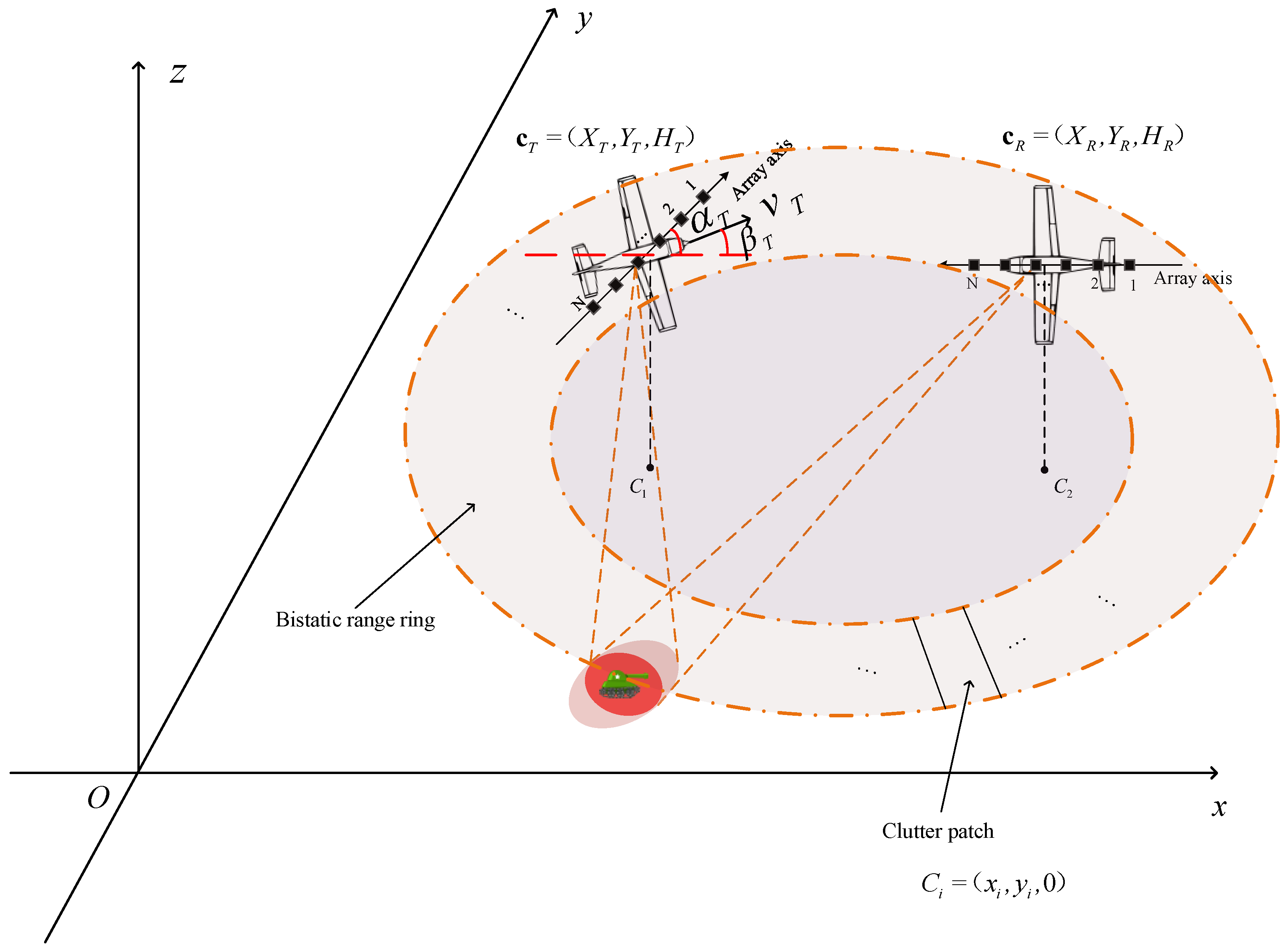
We developed a detailed clutter signal model for airborne bistatic radar.

(2)

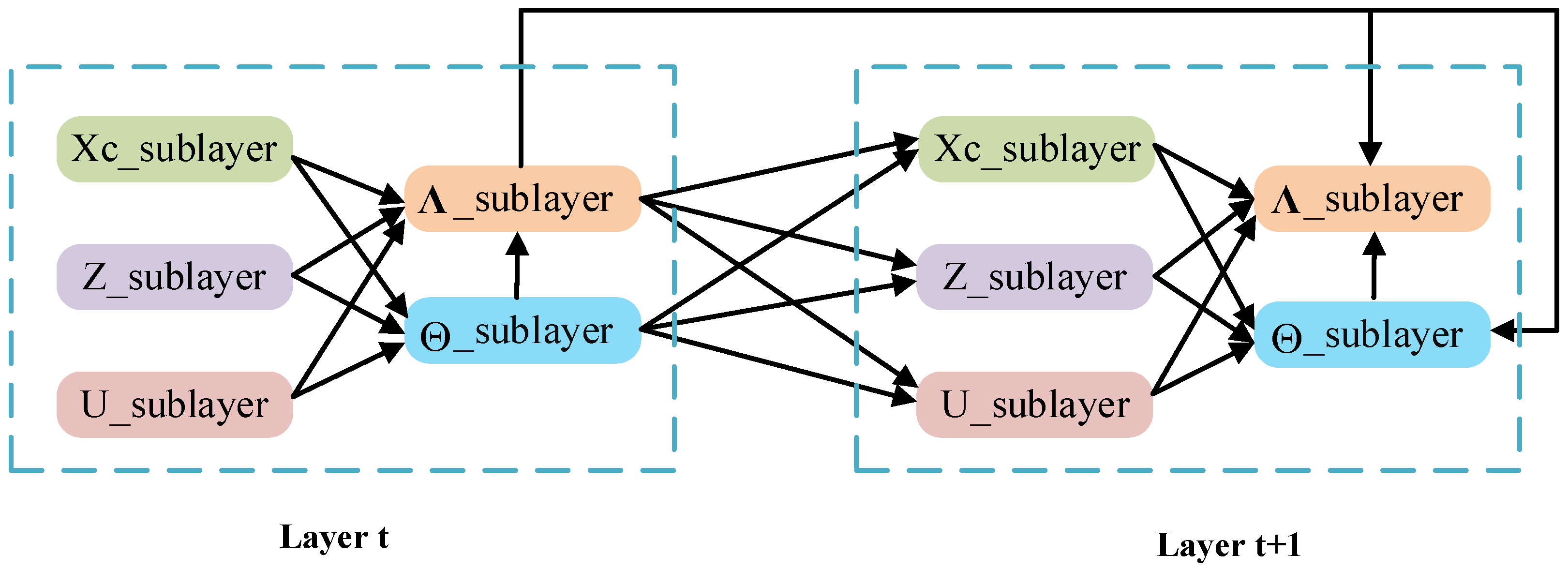
To address the parameter setting difficulties of the ANM algorithm, we unfolded it into a deep neural network, which was called deep unfolding-based gridless sparse recovery bistatic STAP net (DUGLSR-BSTAP-Net). By selecting appropriate training data and labels to calculate the loss function and using the Adam optimizer for backpropagation to update parameters, the network can be trained to set different, more suitable parameters for each layer. This approach contrasts with traditional iterative algorithms, which maintain fixed preset parameters throughout the process.

(3)

We conducted extensive simulation experiments, comparing the proposed algorithm (DUGLSR-BSTAP-Net) with several classic SR-STAP methods across multiple aspects. These aspects included the clutter Capon spectrum, the eigenspectra of the estimated CNCM, improvement factor, and the variation of target detection probability with respect to the signal-to-noise ratio (SNR). The results validated that the proposed algorithm offers superior clutter suppression and target detection performance.

The remainder of this paper is organized as follows.

We establish the clutter model under a bistatic working environment and provide a brief introduction to atomic norm minimization (ANM) in Section 2. Section 3 presents the method for unfolding the iterative process of ANM into a deep neural network. Section 4 conducted comparative experiments on algorithm performance to verify the effectiveness of the proposed algorithm.

Notation: $ℝ$ and $ℂ$ denote the set of real and complex numbers, respectively. $a$, $\mathit{a}$ and $\mathit{A}$ represent a scalar, a vector, and a matrix, respectively. The superscripts ${(\cdot )}^T$ and ${(\cdot )}^H$ are the transpose and conjugate transpose of a vector or matrix.${‖\cdot ‖}_{2,1}$ and ${‖\cdot ‖}_F$ are defined as the ${\mathcal{l}}_{2,1}$ and Frobenius norms. $\otimes$ denotes the Kronecker product. For a vector $\mathit{x}$, diag ($\mathit{x}$) denotes a diagonal matrix with the elements in $\mathit{x}$ on its main diagonal. Tr ($\mathit{A}$) denotes the trace of a matrix $\mathit{A}$. $\mathit{A}\succcurlyeq 0$ means $\mathit{A}$ is a positive semidefinite matrix. The brackets $⌊\cdot ⌋$ indicate rounding to the nearest integer. For matrices $\mathit{A}$ and $\mathit{B}$, $\langle \mathit{A},\mathit{B}\rangle$ = Tr (${\mathit{A}}^H\mathit{B}$). And vec, ($\cdot$) denotes the vectorization operation.

2. Signal Model and Overview of ANM-STAP

In this section, we introduce the airborne bistatic signal model, followed by a brief overview of the ANM-STAP.

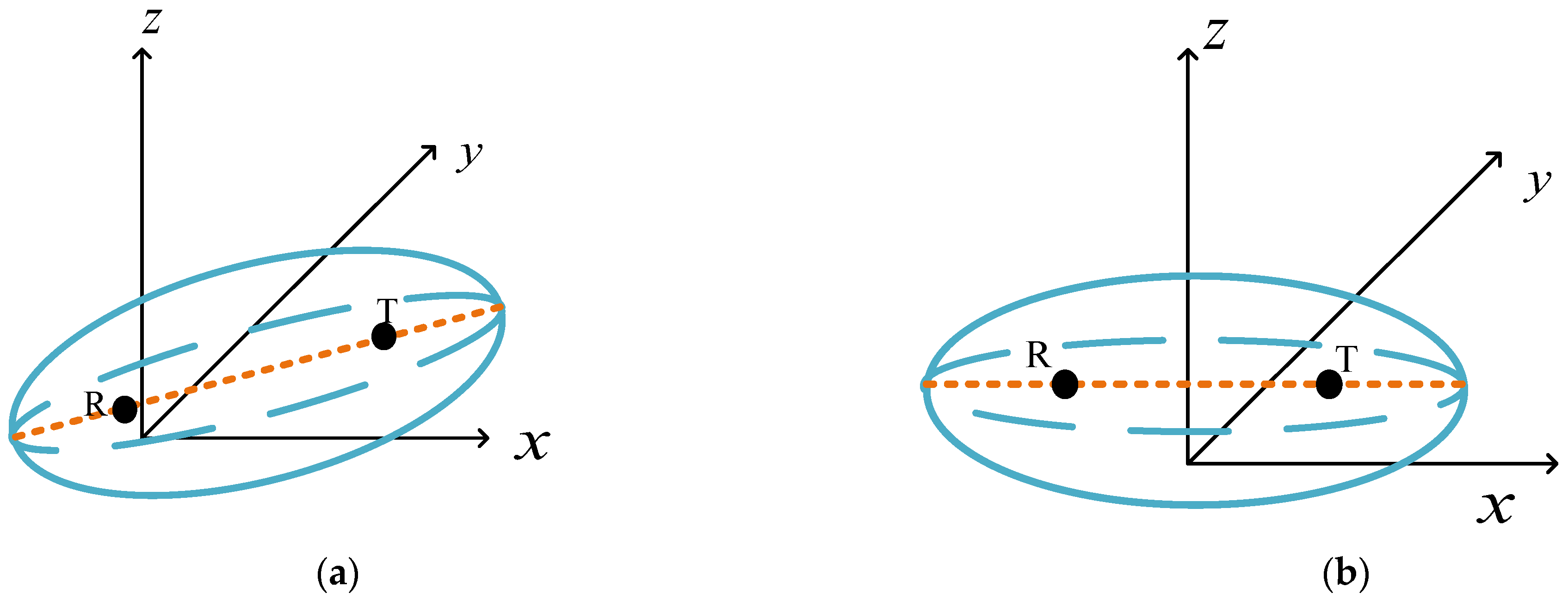
2.1. Airborne Bistatic Signal Model

Consider an airborne bistatic pulsed Doppler radar system featuring a uniformly linear array (ULA) consisting of N elements spaced d apart. Both the transmitter and receiver are equipped with this configuration. The transmitter operates at a constant pulse repetition frequency (PRF) of $f_{PRF}$. Within each coherent processing interval (CPI), the system transmits a coherent burst comprising K pulses. In Figure 1, we established a Cartesian coordinate system, where $c_T=(X_T,Y_T,H_T)$ and $c_R=(X_R,Y_R,H_R)$ represent the spatial coordinates of the transmitter and the receiver, respectively. ${\alpha }_T$ represents the angle between the transmitter’s array axis and the X axis, while ${\beta }_T$ denotes the angle between the direction of the transmitter’s flight velocity and the X axis. In the subsequent sections of the paper, ${\alpha }_R$ and ${\beta }_R$ will, respectively, represent the angle between the receiver’s array axis and the X axis, and the angle between the direction of the receiver’s flight velocity and the X axis (these two angles are not depicted in Figure 1). The set of all scatterers in space for which the sum of the distances to the receiver and transmitter equals a certain value forms a bistatic constant range sum ellipsoid. The intersection of this ellipsoid with the XOY plane is known as the bistatic constant range ring of clutter. In the description, points $C_1$ and $C_2$ represent the ground projections of the transmitter and receiver, respectively.

In practical applications, the center of ellipsoids, defined by the transmitter and receiver as foci, often does not reside on the Z-axis, and the foci are not positioned on the same coordinate axis. Consequently, standard ellipsoidal formulas are not directly applicable for solutions. To address this, this section will implement translation and rotation transformations to align the ellipsoid’s foci on a singular coordinate axis and reposition the ellipsoid’s center onto the Z-axis, as illustrated in Figure 2. By performing these transformations, we can employ the standard ellipsoidal equation to solve for the ellipsoid, thereby accurately determining the coordinates of clutter patches.

First, we need to translate the center of the ellipsoid to the Z-axis. Prior to the translation, the center coordinates are $c_o=\frac{(X_T+X_R,Y_T+Y_R,H_T+H_R)}{2}$, and the coordinates of a point on the ellipsoid surface are $a(x,y,z)$. After the translation, the center coordinates become $c_o=\frac{(0,0,H_T+H_R)}{2}$, and the coordinates of that point on the ellipsoid surface change to be $b(x_B,y_B,z_B)=(x-\mathsf{\Delta }X,y-\mathsf{\Delta }Y,z)$, $\mathsf{\Delta }X=\frac{X_T+X_R}{2},\mathsf{\Delta }Y=\frac{Y_T+Y_R}{2}$. Next, we need to rotate the major axis of the ellipsoid successively around the Z axis and Y axis until it aligns with the X-axis. Let $R_z(a_z)$ and $R_y(a_y)$ be the rotation matrices for rotations around the Z-axis and Y-axis, respectively. The coordinates after rotation are $c(x_C,y_C,z_C)$:

$$\left[\begin{array}{c}{x}_C\\ y_C\\ z_C\end{array}\right]=R_y(a_y)R_z(a_z)\left[\begin{array}{c}{x}_B\\ y_B\\ z_B\end{array}\right]$$

(1)

The coordinate point $c(x_C,y_C,z_C)$ satisfies the standard equation of an ellipsoid:

$$\frac{x_C^2}{a^2}+\frac{y_C^2+z_C^2}{b^2}=1$$

(2)

where a and b, respectively, represent the semi-major and semi-minor axes of the ellipsoid.

For any given l-th range ring with bistatic range $R_l$, the corresponding major and minor axes of the ellipsoid can be determined. According to the definition of an ellipsoid, the semi-major axis a satisfies $2a=R_l$. The semi-focal distance c can be solved based on $2c=\left|c_T-c_R\right|$, and the semi-minor axis b can be determined from the relationship $b^2=a^2-c^2$.

For the rotation matrices $R_z(a_z)$ and $R_y(a_y)$, the sign of the rotation angles should be determined based on the positions of the two foci. In this article, the first rotation is around the Z axis, with a rotation angle of $a_z$. The angle of rotation is from the positive direction of the X-axis towards the positive direction of the Y axis; if the rotation is in the opposite direction, the angle $a_z$ is negative. Specifically, if $(X_T-X_R)\times (Y_T-Y_R)\ge 0$, the rotation angle is negative. The cosine and sine values of the rotation angle are derived from the position coordinates of the focus:

$$\sin a_z=-\frac{\left|Y_T-Y_R\right|}{\sqrt{{(X_T-X_R)}^2+{(Y_T-Y_R)}^2}}$$

(3)

$$\cos a_z=\frac{\left|X_T-X_R\right|}{\sqrt{{(X_T-X_R)}^2+{(Y_T-Y_R)}^2}}$$

(4)

Furthermore, the rotation matrix $R_z(a_z)$ can be expressed as:

$$R_z(a_z)=\left[\begin{array}{ccc}\cos a_z& -\sin a_z& 0\\ \sin a_z& \cos a_z& 0\\ 0& 0& 1\end{array}\right]$$

(5)

Similarly, in the second rotation, when rotating the major axis along the Y axis, the direction of rotation must also be considered when solving for the rotation transformation matrix $R_y(a_y)$. When rotating around the Y-axis, the rotation angle $a_y$ is from the positive direction of the Z-axis towards the positive direction of the X axis; if the rotation is in the opposite direction, the angle $a_y$ is negative. Specifically, if $(X_T-X_R)\times (H_T-H_R)\ge 0$, the rotation angle $a_y$ is positive, and the cosine and sine values of the rotation angle are derived from the position coordinates of the focus:

$$\cos a_y=\frac{\sqrt{{(X_T-X_R)}^2+{(Y_T-Y_R)}^2}}{\sqrt{{(X_T-X_R)}^2+{(Y_T-Y_R)}^2+{(H_T-H_R)}^2}}$$

(6)

$$\sin a_y=-\frac{\left|H_T-H_R\right|}{\sqrt{{(X_T-X_R)}^2+{(Y_T-Y_R)}^2+{(H_T-H_R)}^2}}$$

(7)

Furthermore, the rotation matrix $R_y(a_y)$ can be expressed as:

$$R_y(a_y)=\left[\begin{array}{ccc}\cos a_y& 0& \sin a_y\\ 0& 1& 0\\ -\sin a_y& 0& \cos a_y\end{array}\right]$$

(8)

By substituting Equations (5) and (8) into Equation (1), the coordinates of the position after rotation can be obtained

$$\left[\begin{array}{c}{x}_C\\ y_C\\ z_C\end{array}\right]=R_y(a_y)R_z(a_z)\left[\begin{array}{c}{x}_B\\ y_B\\ z_B\end{array}\right]=\left[\begin{array}{ccc}\cos a_y\cos a_z& -\cos a_y\sin a_z& \sin a_y\\ \sin a_z& \cos a_z& 0\\ -\sin a_y\cos a_z& \sin a_y\sin a_z& \cos a_y\end{array}\right]\left[\begin{array}{c}{x}_B\\ y_B\\ z_B\end{array}\right]$$

(9)

Subsequently, by substituting the coordinates obtained from Equation (9) into Equation (2), and setting z = 0, the formula for the bistatic clutter iso-range contour can be derived:

$$\begin{array}{l}\frac{\begin{array}{l}(x\cos a_y\cos a_z-y\cos a_y\sin a_z-\\ (\mathsf{\Delta }X\cos a_y\cos a_z-\mathsf{\Delta }Y\cos a_y\sin a_z+\mathsf{\Delta }Z\sin a_y){)}^2\end{array}}{a^2}\\ +\frac{{(x\sin a_z+y\cos a_z-(\mathsf{\Delta }X\sin a_z+\mathsf{\Delta }Y\cos a_z))}^2}{b^2}\\ +\frac{\begin{array}{l}(-x\sin a_y\cos a_z+y\sin a_y\sin a_z+\\ (\mathsf{\Delta }X\sin a_y\cos a_z-\mathsf{\Delta }Y\sin a_y\sin a_z-\mathsf{\Delta }Z\cos a_y){)}^2\end{array}}{b^2}=1\end{array}$$

(10)

Using polar coordinates, any point on the ground can be represented as:

$$\left\{\begin{array}{l}x=r\cos \theta \\ y=r\sin \theta \end{array}\right.$$

(11)

By substituting Equation (11) into Equation (10) and transforming it into polar coordinates, the equation can be simplified and rearranged to obtain:

$$\begin{array}{l}{r}^2(b^2{M}_1^2+a^2{M}_2^2+a^2{M}_3^2)+\\ r(-2(b^2{M}_1{C}_1+a^2{M}_2{C}_2+a^2{M}_3{C}_3))+\\ b^2{C}_1^2+a^2{C}_2^2+a^2{C}_3^2-a^2{b}^2=0\end{array}$$

(12)

The symbols in the above equation are defined as follows:

$$\begin{array}{l}{C}_1=\mathsf{\Delta }X\cos a_y\cos a_z-\mathsf{\Delta }Y\cos a_y\sin a_z+\mathsf{\Delta }Z\sin a_y\\ C_2=\mathsf{\Delta }X\sin a_z+\mathsf{\Delta }Y\cos a_z\\ C_3=\mathsf{\Delta }X\sin a_y\cos a_z-\mathsf{\Delta }Y\sin a_y\sin a_z-\mathsf{\Delta }Z\cos a_y\\ M_1=\cos \theta \cos a_y\cos a_z-\sin \theta \cos a_y\sin a_z\\ M_2=\cos \theta \sin a_z+\sin \theta \cos a_z\\ M_3=\cos \theta \sin a_y\cos a_z-\sin \theta \sin a_y\sin a_z\end{array}$$

(13)

By simplifying the coefficients of Equation (12) and rearranging the equation, the following can be derived:

$$\begin{array}{l}{A}_1=(b^2{M}_1^2+a^2{M}_2^2+a^2{M}_3^2)\\ A_2=-2(b^2{M}_1{C}_1+a^2{M}_2{C}_2+a^2{M}_3{C}_3)\\ A_3=b^2{C}_1^2+a^2{C}_2^2+a^2{C}_3^2-a^2{b}^2\\ r^2{A}_1+r{A}_2+A_3=0\end{array}$$

(14)

Solving the above equation can yield the coordinates of the clutter patch:

$$\left\{\begin{array}{l}{r}_1=\frac{-A_2+\sqrt{{A_2}^2-4A_3{A}_1}}{2A_1}\\ r_2=\frac{-A_2-\sqrt{{A_2}^2-4A_3{A}_1}}{2A_1}\end{array}\right.$$

(15)

$$\left\{\begin{array}{l}(x_1,y_1,0)=(r_1\cos \theta ,r_1\sin \theta ,0)\\ (x_2,y_2,0)=(r_2\cos \theta ,r_2\sin \theta ,0)\end{array}\right.$$

(16)

After conducting numerous experiments, we found that $r_2$ is always less than zero, and needs to be discarded.

In summary, when a bistatic range is specified, a unique polar radius can be obtained. By combining this with the angle $\theta$, we can determine the coordinates of each clutter patch.

$$(x_i,y_i,0)=(r_1\cos \theta ,r_1\sin \theta ,0)$$

(17)

From Figure 1, we can see that the axial direction vector of the receiver’s array is $d_r=(\cos {\alpha }_r,\sin {\alpha }_r,0)$, the velocity direction vector is $v_r=(\cos {\beta }_r,\sin {\beta }_r,0)$, and the direction vectors of the transmitter and receiver relative to the clutter block connection line are, respectively, $c_t=(x_i-X_T,y_i-Y_T,-H_T)$ and $c_r=(x_i-X_R,y_i-Y_R,-H_R)$.

Based on this, the expressions for the velocity cone angles and spatial cone angles of this clutter patch are:

$$\cos {\phi }_R=\frac{<c_r,d_r>}{\left|c_r\right|\left|d_r\right|}=\frac{(x_i-X_R)\cos {\beta }_r+(y_i-Y_R)\sin {\beta }_r}{\sqrt{{(x_i-X_R)}^2+{(y_i-Y_R)}^2+{H_R}^2}}$$

(18)

$$\cos {\psi }_R=\frac{<v_{r,}{c}_r>}{\left|v_r\right|\left|c_r\right|}=\frac{(x_i-X_R)\cos {\alpha }_r+(y_i-Y_R)\sin {\alpha }_r}{\sqrt{{(x_i-X_R)}^2+{(y_i-Y_R)}^2+{H_R}^2}}$$

(19)

$$\cos {\psi }_T=\frac{<v_t,c_t>}{\left|v_t\right|\left|c_t\right|}=\frac{(x_i-X_T)\cos {\alpha }_t+(y_i-Y_T)\sin {\alpha }_t}{\sqrt{{(x_i-X_T)}^2+{(y_i-Y_T)}^2+{H_T}^2}}$$

(20)

In the above expression, $\cos {\phi }_R$ represents the spatial cone angle of the receiver, $\cos {\psi }_R$ represents the velocity cone angle of the receiver, and $\cos {\psi }_T$ represents the velocity cone angle of the transmitter. Assuming that the array is an equidistant linear array and the spacing between the elements is d the spatial frequency of the clutter patch received can be derived from the receiver’s spatial cone angle:

$$f_{si}=\frac{d\cos {\phi }_R}{\lambda }$$

(21)

where $\lambda$ is the wavelength, and d is the inter-element interval. Combining (19), (20), and the magnitudes of the velocities of the transmitter and receiver, the normalized Doppler frequency of the clutter patch can be determined:

$$f_{di}=\frac{v_t\cos {\psi }_T}{\lambda f_{PRF}}+\frac{v_r\cos {\psi }_R}{\lambda f_{PRF}}$$

(22)

with the derivations above, we can logically deduce the space–time steering vector of the clutter block:

$$s(f_{s_i},f_{d_i})=s_t(f_{d_i})\otimes s_s(f_{s_i})$$

(23)

where $s_s(f_{s_i})={\left[1,e^{j2\pi f_{s_i}},\cdots ,e^{j2\pi (N-1)f_{s_i}}\right]}^T$ and $s_t(f_{d_i})={\left[1,e^{j2\pi f_{d_i}},\cdots ,e^{j2\pi (K-1)f_{d_i}}\right]}^T$ denote the spatial and temporal steering vector, respectively.

From the above derivation, it can be concluded that the clutter Doppler frequency in airborne bistatic radar is determined by both the transmitter and receiver, while the spatial frequency is solely determined by the receiver. This results in more complex space-time characteristics of the clutter. Figure 3 illustrates the space–time characteristics of the clutter under four different bistatic configurations. When using grid-based sparse recovery algorithms, a significant amount of clutter does not fall on the pre-divided space–time grid points, leading to severe grid mismatch and consequently degrading the algorithm’s performance.

Based on the Ward report [4], the clutter component at each range ring can be envisioned as a superposition of uniformly distributed and independent clutter patches. Consequently, it can be articulated as follows:

$$x_c={\displaystyle \sum _{i=1}^{N_c}{\alpha }_i\left(s_s(f_{s_i})\otimes s_t(f_{d_i})\right)}={\displaystyle \sum _{i=1}^{N_c}{\alpha }_{i}s(f_{s_i},f_{d_i})}$$

(24)

When the target is absent in the scenarios, the received space–time snapshot consists solely of the clutter signal and thermal noise.

$$x=x_c+n$$

(25)

where the noise vector $n$ is represented as white Gaussian noise with zero mean and covariance matrix $E\left\{n{n}^H\right\}={\sigma }^{2}I$, and ${\sigma }^2$ denotes the noise variance.

The clutter plus noise covariance matrix (CNCM) can be estimated by:

$$R\triangleq E\left\{x{x}^H\right\}={\displaystyle \sum _{i=1}^{N_c}E\left\{{\left|{\alpha }_i\right|}^2\right\}s(f_{s_i},f_{d_i})s^H(f_{s_i},f_{d_i})}+{\sigma }^{2}I=R_c+{\sigma }^{2}I$$

(26)

can be given by $\widehat{R}=\frac{1}{L}{\displaystyle \sum _{l=1}^L{x}_l{x}_l^H}$, where $L$ denotes the amounts of available IID training samples and $x_l$ is the snapshot of the l-th training range ring, $R_c$ is the clutter covariance matrix. In accordance with the maximum signal-to-interference-plus-noise ratio (SINR) criterion [2], the derivation of the sample matrix inversion (SMI) weight vector for the space–time adaptive processing (STAP) filter can be systematically established:

$$w_{SMI}=\frac{{\widehat{R}}^{-1}{s}_T}{{s_T}^H{\widehat{R}}^{-1}{s}_T}$$

(27)

where $s_T$ denotes the target spatial-temporal steering vector.

2.2. ANM-STAP

Employing grid-based sparse recovery algorithms for the suppression of bistatic clutter often results in substantial performance degradation due to grid mismatch issues. To resolve these challenges from their root, it is imperative to utilize gridless sparse recovery algorithms. The concept of ANM-STAP was initially proposed in [16] as a solution to counteract the off-grid effect. In contrast to grid-based algorithms, the core principle of gridless SR-STAP is to represent the clutter subspace through a linear combination of selected atoms from a predefined, continuous spatial-temporal atom set. Based on (24), this approach utilizes an infinite set of atoms defined as follows:

$$\mathcal{A}\triangleq \left\{s(f_s,f_d){\beta }^T|f_s,f_d\in \left[-0.5,0.5\right),{‖\beta ‖}_2=1\right\}$$

(28)

Reference [23] states that, the pure clutter signal matrix, consisting of L snapshots, can be succinctly represented by a few specific atoms within $\mathcal{A}$, as demonstrated by the subsequent linear combination.

$$X_c={\displaystyle \sum _{r=1}^{N_r}s(f_{s,r},f_{d,r})[{\beta }_r^1,{\beta }_r^2,\cdots ,{\beta }_r^L]}={\displaystyle \sum _{r=1}^{N_r}{\chi }_{r}s(f_{s,r},f_{d,r}){\beta }_r^T}$$

(29)

where $N_r$ denotes the clutter rank, indicating that the clutter subspace is spanned by merely $N_r$ space–time steering vectors, and here, we define ${\beta }_r^0={[{\beta }_r^1,{\beta }_r^2,\cdots ,{\beta }_r^L]}^T$, ${\chi }_r={‖{\beta }_r^0‖}_2$ and ${\beta }_r={\beta }_r^0/{\chi }_r$. Within the ANM-STAP framework, the atomic norm of $X_c$ relative to the atom set is defined by the following infimum

$${‖X_c‖}_{\mathcal{A}}\triangleq \inf \left\{\left.{\displaystyle \sum _r\left|{\chi }_r\right|}\right|X_c={\displaystyle \sum _r{\chi }_{r}s(f_{s,r},f_{d,r}){\beta }_r^T}\right\}$$

(30)

which seeks the sparsest representation of $X_c$ over $\mathcal{A}$.

The computation of the atomic norm is inherently complex. However, in the specific context of the uniform linear array (ULA) operating under a invariant pulse repetition frequency, both spatial and temporal steering vectors manifest a Vandermonde structure. Exploiting the intrinsic Toeplitz-block-Toeplitz architecture of the CNCM, the calculation of the atomic norm delineated in (30) can be accurately executed via the proposed semidefinite programming (SDP) framework [15].

$$\underset{Z,U,X_c}{\min }+\mathrm{Tr}(Z)+\mathrm{Tr}(L\mathcal{T}(U))+\frac{{\lambda }_{\mathcal{A}}}{2}{‖X-X_c‖}_F^2\hspace{1em}s.t. \Theta = \left[\begin{array}{cc}Z& X_c^H\\ X_c& L\mathcal{T}(U)\end{array}\right]\succcurlyeq 0 , Z=Z^H$$

(31)

In this formulation, ${\lambda }_{\mathcal{A}}>0$ is the regularization parameter, $Z={\displaystyle \sum _{r=1}^{N_r}{\beta }_r·{({\beta }_r)}^H}\in {ℂ}^{L\times L}$,$U$ refers to a complex matrix of dimensions (2N − 1) × (2K − 1). Additionally, $\mathcal{T}(U)\subset {ℂ}^{NK\times NK}$ denotes the parametric representation of $R_c$ that capitalizes on the block-Toeplitz characteristic.

$$\mathcal{T}(U)=\left[\begin{array}{cccc}{U}_0& U_{-1}& \cdots & U_{-N+1}\\ U_1& U_0& \cdots & U_{-N+2}\\ ⋮& ⋮& \ddots & ⋮\\ U_{N-1}& U_{N-2}& \cdots & U_0\end{array}\right]$$

(32)

$$U_n=\left[\begin{array}{cccc}{U}_{n,0}& U_{n,-1}& \cdots & U_{n,-K+1}\\ U_{n,1}& U_{n,0}& \cdots & U_{n,-K+2}\\ ⋮& ⋮& \ddots & ⋮\\ U_{n,K-1}& U_{n,K-2}& \cdots & U_0\end{array}\right]$$

(33)

where each inner block $U_n$ ($-N<n<N$) is an $K\times K$ Toeplitz matrix defined from the nth row of $U$.

The above optimization problem in (31) is termed as ANM-STAP and can be solved using the ADMM [24] (alternating direction method of multipliers) algorithm. When $\widehat{U}$ is obtained, the estimated CNCM can then be reconstructed by

$${\widehat{R}}_{sr}=\frac{1}{L}{\displaystyle \sum _{l=1}^L\widehat{\Gamma }diag\left({\left|{\widehat{\Gamma }}^{-1}{x}_l\right|}^2\right)}{\widehat{\Gamma }}^H+{\sigma }^{2}I$$

(34)

where $\widehat{\Gamma }\in {ℂ}^{NK\times NK}$ is a matrix whose columns are composed of the eigenvectors of $\mathcal{T}(\widehat{U})$. Substituting this into (27) results in the derivation of the weight vector for the ANM-STAP methodology.

In this section, we introduced the signal model of the airborne bistatic radar and the related concepts of gridless SR-STAP, laying the groundwork for our subsequent application of deep unfolding networks to solve (31).

3. Unfolding Gridless Sparse Recovery Bistatic STAP Algorithms into Deep Networks

Moving forward, in this section, we will propose an innovative deep unfolding-based gridless sparse recovery bistatic STAP net (DUGLSR-BSTAP-Net) whose clutter suppression performance surpasses that of some current mainstream sparse recovery algorithms.

3.1. Gridless Sparse Recovery Bistatic STAP(GLSR-BSTAP)

First of all, we describe how to apply the ADMM [24] to solve (31). The augmented Lagrangian expression for Equation (31) is defined as follows.

$$\begin{array}{l}\mathcal{L}(X_c,U,Z,\Theta ,\Lambda )\\ =\mathrm{T}r(L\mathcal{T}(U))+\mathrm{T}r(Z)+\frac{{\lambda }_{\mathcal{A}}}{2}{‖X-X_c‖}_F^2\\ +〈\Lambda ,\Theta -\left[\begin{array}{cc}Z& {X_c}^H\\ X_c& \mathcal{L}\mathcal{T}(U)\end{array}\right]〉\\ +\frac{\rho }{2}{‖\Theta -\left[\begin{array}{cc}Z& {X_c}^H\\ X_c& \mathcal{L}\mathcal{T}(U)\end{array}\right]‖}_F^2\\ \end{array}$$

(35)

where $\Lambda \in {ℂ}^{(NK+L)\times (NK+L)}$ is the Lagrangian multiplier, $\rho >0$ is a penalty parameter. Before beginning the iterations, both $\Theta$ and $\Lambda$ are initialized as zero matrices.

(1)

Update $X_C^{t+1},U^{t+1},Z^{t+1}$:

$$(X_C^{t+1},U^{t+1},Z^{t+1})=\underset{X_C,U,Z}{\arg \min }(\mathcal{L}(X_C,U,Z,{\Theta }^t,{\Lambda }^t))$$

(36)

We partition the matrices ${\Theta }^t$ and ${\Lambda }^t$ as follows:

$${\Theta }^t=\left[\begin{array}{cc}{\Theta }_Z^t& {({\Theta }_{X_C}^t)}^H\\ {\Theta }_{X_C}^t& {\Theta }_{\mathcal{T}(U)}^t\end{array}\right]$$

(37)

$${\Lambda }^t=\left[\begin{array}{cc}{\Lambda }_Z^t& {({\Lambda }_{X_C}^t)}^H\\ {\Lambda }_{X_C}^t& {\Lambda }_{\mathcal{T}(U)}^t\end{array}\right]$$

(38)

where ${\Theta }_Z^t$ and ${\Lambda }_Z^t$ are L × L matrices, ${\Theta }_{X_C}^t$ and ${\Lambda }_{X_C}^t$ are NK × L matrices, and ${\Theta }_{\mathcal{T}(U)}^t$ and ${\Lambda }_{\mathcal{T}(U)}^t$ are NK × NK matrices.

Calculating the partial derivatives of Equation (36) with respect to $X_c$, $Z$, and $\mathcal{T}(U)$, respectively, yields the following results

$$\frac{\partial \mathcal{L}(X_C,U,Z,{\Theta }^t,{\Lambda }^t)}{\partial X_C}=-{\lambda }_{\mathcal{A}}X-2{\Lambda }_{X_C}^t-2\rho {\Theta }_{X_C}^t+(2\rho +{\lambda }_{\mathcal{A}})X_C$$

(39)

$$\frac{\partial \mathcal{L}(X_C,U,Z,{\Theta }^t,{\Lambda }^t)}{\partial Z}=I_L-{\Lambda }_Z^t-\rho {\Theta }_Z^t+\rho Z$$

(40)

$$\frac{\partial \mathcal{L}(X_C,U,Z,{\Theta }^t,{\Lambda }^t)}{\partial \mathcal{T}(U)}=L{I}_{NK}-L{\Lambda }_{\mathcal{T}(U)}^t-\rho L{\Theta }_{\mathcal{T}(U)}^t+\rho L^2\mathcal{T}(U)$$

(41)

Let (39)–(41) be 0, we then have

$$X_C^{t+1}=\frac{1}{(2\rho +{\lambda }_{\mathcal{A}})}({\lambda }_{\mathcal{A}}X+2{\Lambda }_{X_C}^t+2\rho {\Theta }_{X_C}^t)$$

(42)

$$Z^{t+1}={\rho }^{-1}{\Lambda }_z^t+{\Theta }_z^t-{\rho }^{-1}{I}_L$$

(43)

$${(\mathcal{T}(U))}^{t+1}={(\rho L)}^{-1}{\Lambda }_{\mathcal{T}(U)}^t+L^{-1}{\Theta }_{\mathcal{T}(U)}^t-{(\rho L)}^{-1}{I}_{NK}$$

(44)

By leveraging Equation (44) along with the previously established block-Toeplitz property of ${(\mathcal{T}(U))}^{t+1}$, we can derive the following

$${(U)}^{t+1}={\mathcal{T}}^{*}({(\rho L)}^{-1}{\Lambda }_{\mathcal{T}(U)}^t+L^{-1}{\Theta }_{\mathcal{T}(U)}^t)-{(\rho L)}^{-1}{E}_{N,K}$$

(45)

where $E_{N,K}$ is a (2N − 1) × (2K − 1) matrix with the (N, K)-th element being 1 and others being 0. Additionally, the symbol ${\mathcal{T}}^{*}(·)$ in (32) is a mapping from a NK × NK matrix to a (2N − 1) × (2K − 1) matrix.

(2)

Update ${\Theta }^{t+1}$:

$$\begin{array}{ll}{\Theta }^{t+1}& =\underset{\Theta \succcurlyeq 0}{\arg \min }\mathcal{L}(X_C^{t+1},U^{t+1},Z^{t+1},\Theta ,{\Lambda }^t)\\ & =\underset{\Theta \succcurlyeq 0}{\arg \min }\frac{\rho }{2}{‖\Theta -\left[\begin{array}{cc}{Z}^{t+1}& {(X_C^{t+1})}^H\\ X_C^{t+1}& L\mathcal{T}(U^{t+1})\end{array}\right]+{\rho }^{-1}{\Lambda }^t‖}_F^2\end{array}$$

(46)

Clearly, the optimal solution to Equation (46) in the absence of the constraint $\Theta \succcurlyeq 0$ is

$${\Theta }_{un}^{t+1}=\left[\begin{array}{cc}{Z}^{t+1}& {(X_C^{t+1})}^H\\ X_C^{t+1}& L\mathcal{T}(U^{t+1})\end{array}\right]-{\rho }^{-1}{\Lambda }^t$$

(47)

Let ${\Theta }_{un}^{t+1}=Gdiag(\{{\delta }_g\})G^{-1}, \mathrm{g}=1,2,\mathrm{\dots },NK+L$, and set all negative eigenvalues to zero that we can have the updating result

$$\left\{\begin{array}{l}{\Theta }_{un}^{t+1}=\left[\begin{array}{cc}{Z}^{t+1}& {(X_C^{t+1})}^H\\ X_C^{t+1}& L\mathcal{T}(U^{t+1})\end{array}\right]-{\rho }^{-1}{\Lambda }^t\\ {\Theta }_{un}^{t+1}=Gdiag(\{{\delta }_g\})G^{-1}, \mathrm{g}=1,2,\mathrm{\dots },NK+L\\ {\Theta }^{t+1}=Gdiag({\left\{{\delta }_g\right\}}_{+})G^{-1}\end{array}\right.$$

(48)

(3)

Update ${\Lambda }^{t+1}$:

Finally, we can update ${\Lambda }^{t+1}$ by

$${\Lambda }^{t+1}={\Lambda }^t+\rho \left({\Theta }^{t+1}-\left[\begin{array}{cc}{Z}^{t+1}& {(X_C^{t+1})}^H\\ X_C^{t+1}& L\mathcal{T}(U^{t+1})\end{array}\right]\right)$$

(49)

The aforementioned algorithm exhibits two primary limitations: Firstly, the Lagrangian multiplier $\Lambda$ and penalty parameter $\rho$ require predefined settings, which, if not judiciously chosen, can lead to substantial declines in algorithm performance. Secondly, throughout the iterative execution of the algorithm, ${\lambda }_{\mathcal{A}}$ and $\rho$ remain fixed, thereby inhibiting the adaptive recalibration of these parameters in response to suboptimal initial settings. The proposed DU-GLSR-BSTAP can perfectly address the aforementioned issues, effectively achieving the suppression of bistatic clutter.

3.2. DUGLSR-BSTAP-Net

Figure 4 presents a clear and accessible depiction of the deep unfolding network. Each iteration of the traditional algorithm (left) is represented as one layer of the network (right). Concatenating these layers forms a deep neural network, and as data pass through this network, these effectively replicate the process of running the iterative algorithm multiple times. Furthermore, algorithmic parameters, including model parameters and regularization coefficients, are transformed into network parameters. The network can be trained via back-propagation, enabling the learning of model parameters from real-world training datasets. Consequently, the trained network can be viewed as a parameter-optimized algorithm, which effectively overcomes the two issues present in the GLSR-BSTAP algorithm by enabling the adaptive correction of suboptimal parameter presets and deploying distinct parameters for each network layer.

We define a DUGLSR-BSTAP-Net to solve Equation (31). As depicted in Figure 5, each layer of the network comprises five sub-layers, corresponding to (42), (43), (45), (48), and (49), respectively, named Xc-sublayer, Z_sublayer, U_sublayer, $\Theta$_sublayer, and $\Lambda$_sublayer.

In the (t + 1)-th layer of the network, each sub-layer extracts the data required for its computations from the output “Data Package” of the t-th layer, facilitating the forward propagation in the t-th layer.

(1) Reconstruction sublayer—Xc_sublayer^(t+1): Using the outputs ${\Lambda }_{Xc}^t$ from sub-layer $\Lambda \_{\mathrm{sublayer}}^{(t)}$ and ${\Theta }_{Xc}^t$ from sub-layer $\Theta \_{\mathrm{sublayer}}^{(t)}$ of the t-th layer, along with the received signal X as inputs, the output $X_C^{t+1}$ is updated accordingly.

$$X_C^{t+1}=\frac{1}{(2\rho +{\lambda }_{\mathcal{A}})}({\lambda }_{\mathcal{A}}X+2{\Lambda }_{X_C}^t+2\rho {\Theta }_{X_C}^t)$$

(50)

(2) Auxiliary variable update sublayer—Z_sublayer^(t+1): Taking the outputs ${\Lambda }_Z^t$ and ${\Theta }_Z^t$ from sub-layers $\Lambda \_{\mathrm{sublayer}}^{(t)}$ and $\Theta \_{\mathrm{sublayer}}^{(t)}$, respectively, in the t-th layer, the subsequent output $Z^{t+1}$ is then updated.

$$Z^{t+1}={\rho }^{-1}{\Lambda }_z^t+{\Theta }_z^t-{\rho }^{-1}{I}_L$$

(51)

(3) Parametric CCM update sublayer—U_sublayer^(t+1): Using the outputs ${\Lambda }_{\mathcal{T}(U)}^t$ from sub-layer $\Lambda \_{\mathrm{sublayer}}^{(t)}$ and ${\Theta }_{\mathcal{T}(U)}^t$ from sub-layer $\Theta \_{\mathrm{sublayer}}^{(t)}$ of the t-th layer, the output ${(U)}^{t+1}$ is updated accordingly.

$${(U)}^{t+1}={\mathcal{T}}^{*}({(\rho L)}^{-1}{\Lambda }_{\mathcal{T}(U)}^t+L^{-1}{\Theta }_{\mathcal{T}(U)}^t)-{(\rho L)}^{-1}{E}_{N,K}$$

(52)

(4) Nonlinear activation sublayer—${\Theta \_sublayer}^{(\mathrm{t}+1)}$: Taking the outputs $X_C^{t+1}$, $Z^{t+1}$, $\mathcal{T}(U^{t+1})$ from the sub-layers ${\mathrm{X}}_{\mathrm{C}}{\text{\_}\mathrm{sublayer}}^{(t+1)}$, ${\mathrm{Z}\text{\_}\mathrm{sublayer}}^{(t+1)}$, ${\mathrm{U}\text{\_}\mathrm{sublayer}}^{(t+1)}$, respectively, in the (t + 1)-th layer and ${\Lambda }^t$ from $\Lambda \_{\mathrm{sublayer}}^{(t)}$ in the t-th layer, the subsequent output ${\Theta }^{t+1}$ is then updated

$$\left\{\begin{array}{l}{\Theta }_{un}^{t+1}=\left[\begin{array}{cc}{Z}^{t+1}& {(X_C^{t+1})}^H\\ X_C^{t+1}& L\mathcal{T}(U^{t+1})\end{array}\right]-{\rho }^{-1}{\Lambda }^t\\ {\Theta }_{un}^{t+1}=Gdiag(\{{\delta }_g\})G^{-1}, \mathrm{g}=1,2,\mathrm{\dots },NK+L\\ {\Theta }^{t+1}=Gdiag({\left\{{\delta }_g\right\}}_{+})G^{-1}\end{array}\right.$$

(53)

(5) Lagrangian multiplier update sublayer—${\Lambda \_sublayer}^{(\mathrm{t}+1)}$: Taking the outputs $X_C^{t+1}$, $Z^{t+1}$, $\mathcal{T}(U^{t+1})$ from sub-layers ${\mathrm{X}}_{\mathrm{C}}{\text{\_}\mathrm{sublayer}}^{(t+1)}$, ${\mathrm{Z}\text{\_}\mathrm{sublayer}}^{(t+1)}$, ${\mathrm{U}\text{\_}\mathrm{sublayer}}^{(t+1)}$, respectively, in the (t + 1)-th layer and ${\Lambda }^t$ from $\Lambda \_{\mathrm{sublayer}}^{(t)}$ in the t-th layer, the subsequent output ${\Theta }^{t+1}$ is then updated

$${\Lambda }^{t+1}={\Lambda }^t+\rho \left({\Theta }^{t+1}-\left[\begin{array}{cc}{Z}^{t+1}& {(X_C^{t+1})}^H\\ X_C^{t+1}& L\mathcal{T}(U^{t+1})\end{array}\right]\right)$$

(54)

3.3. Network Structure Analysis

Compared to traditional convolutional neural networks, the proposed DUGLSR-BSTAP-Net has the following similarities and differences.

(1): Unlike convolutional neural networks, proposed DUGLSR-BSTAP-Net inherently integrate physical domain knowledge into CNCM reconstruction. The operation in the reconstruction sublayer is a crucial step for performing the inverse mapping from a received signal to the reconstructed clutter component. The auxiliary variable update sublayer contains information related to the coefficients of the atoms that span the clutter subspace. The parametric CCM update sublayer exists to compute T(U), which is the parameterized representation of the CCM. Similar to CNNs, the nonlinear activation sublayer introduces non-linear activation capability to the network when computing the constraint term $\Theta$.

(2): Additionally, proposed net feature skip connections are shown in Figure 6. For example, the nonlinear activation sublayer and Lagrangian multiplier update sublayer form short connections between the reconstruction sublayer, auxiliary variable update sublayer, and parametric CCM update sublayer across various layers. Moreover, the Lagrangian multiplier update sublayer naturally connects to themselves through gradient descent updates. This approach is similar to the residual network [25] where skip connections have been demonstrated to be effective for training very deep neural networks. Our networks also utilize skip connections, but these are inherently determined by ADMM iterative algorithm.

3.4. Generating the Training Dataset

This network employs a supervised training approach, utilizing the training dataset obtained through the simulation of the model introduced in Section 2, which includes both inputs and labels. In practical applications, it is assumed that certain characteristics of the radar system are adequately known. Although the reflectivity of the ground at each clutter patch is naturally random, it adheres to a specific distribution influenced by factors such as terrain type, radar frequency, and polarization. We divided each bistatic equal range ellipse into 720 clutter patches, corresponding to θ in Equation (17), ranging from 0° to 360°. Using Equation (17), we calculated the spatial coordinates of each clutter patch. With the known positions of the transmitter and receiver, we applied Equations (18)–(20) to determine the array cone angle and velocity cone angle of each clutter patch relative to the receiver, as well as the velocity cone angle relative to the transmitter. This allowed us to derive the spatial frequency (Equation (21)) and Doppler frequency (Equation (22)), and subsequently compute the space–time steering vector (Equation (23)). Using the radar equation, we calculated the power of each clutter patch, with a −30 dB power loss for those located in the receiver’s backlobe. To simulate the fluctuations of clutter patches in a real environment, we assigned each patch a complex random number following a standard normal distribution. We simulated 3200 samples from different range gates, encompassing four different bistatic configurations. Each range gate represents a different elevation angle. At the same time, due to the highly non-stationary nature of airborne bistatic clutter, the clutter characteristics vary across different range gates, thus avoiding uniformity in the training data. Among them, 2560 samples are used for training, and 640 samples are used for testing.

Based on this, we can have the input dataset ${\left\{X_q\right\}}_{q=1}^Q$, Q is the amount of training samples. The goal of STAP is to effectively suppress clutter, and the improvement factor (IF) serves as a valuable measure for evaluating the clutter suppression performance of an algorithm.

$$\mathrm{IF}=\frac{\mathrm{Tr}(R)}{NK}\frac{{\left|w^H{s}^T(f_s,f_d)\right|}^2}{w^{H}Rw}$$

(55)

where $R$ is the clairvoyant CNCM of the CUT is known as a prior via simulation, $s^T(f_s,f_d)$ is the practical target spatial-temporal steering vector.

Therefore, we will use the IF calculated using the weight vector derived from the clairvoyant CNCM through Equation (27) as our label dataset ${\left\{Y_q\right\}}_{q=1}^Q$.

3.5. Network Initialization and Training Method

For network initialization settings, we set the initial values with ${\lambda }_{\mathcal{A}}=0.5$ and $\rho =0.01$ in each layer. The normalized mean squared error (NMSE) is utilized as the loss function. When received signal pass the DUGLSR-BSTAP-Net is completed, we obtain the output $\mathcal{T}(\widehat{U})$. Using Equation (34), we compute the CNCM, and subsequently derive the weights through Equation (27). These weights are then applied in Equation (55) to calculate the IF, ${\left\{F_q({\lambda }_{\mathcal{A}},\rho ;X_q)\right\}}_{q=1}^Q$. This result is incorporated into the loss function calculation, after which the parameters are updated using the Adam [26] optimizer, completing one training cycle.

$$L({\lambda }_{\mathcal{A}},\rho )=\frac{1}{Q}{\displaystyle \sum _{q=1}^Q\frac{{‖Y_q-F_q({\lambda }_{\mathcal{A}},\rho ;X_q)‖}_F^2}{{‖Y_q‖}_F^2}}$$

(56)

4. Numerical Simulations

In this section, we evaluate the performance of the newly proposed DUGLSR-BSTAP-Net algorithm through extensive simulation experiments. We conduct thorough comparisons using various advanced SR-STAP algorithms, such as the grid-based MIAA [9], MSBL [11], MOMP [27], and MFOCUSS [28], and gridles ANM [29] and last but not least, the optimal STAP filter. The available number of IID training samples is twelve. The main simulation parameters are listed in

Table 1. Parameters of airborne bistatic radar system.

Parameter	Value	Unit
Number of transmitter and receiver array element N	8	-
Number of pulses K	8	-
Pulse repetition frequency $f_{PRF}$	2000	Hz
$\lambda$	0.3	m
Bandwidth	2.5	MHz
Velocity of transmitter and receiver	120	m/s
CNR	40	dB

. The DUGLSR-BSTAP-Net was trained on an Intel(R) Xeon(R) Gold 6258R CPU @ 2.70 GHz 2.69 GHz (two processors) and an NVIDIA Quadro RTX 8000 GPU. The Intel Xeon CPU is manufactured by Intel Corporation, located in Santa Clara, CA, USA. The NVIDIA Quadro RTX 8000 GPU is manufactured by NVIDIA Corporation, also located in Santa Clara, CA, USA. The training environment utilized Python 3.8 and Pytorch 1.8.

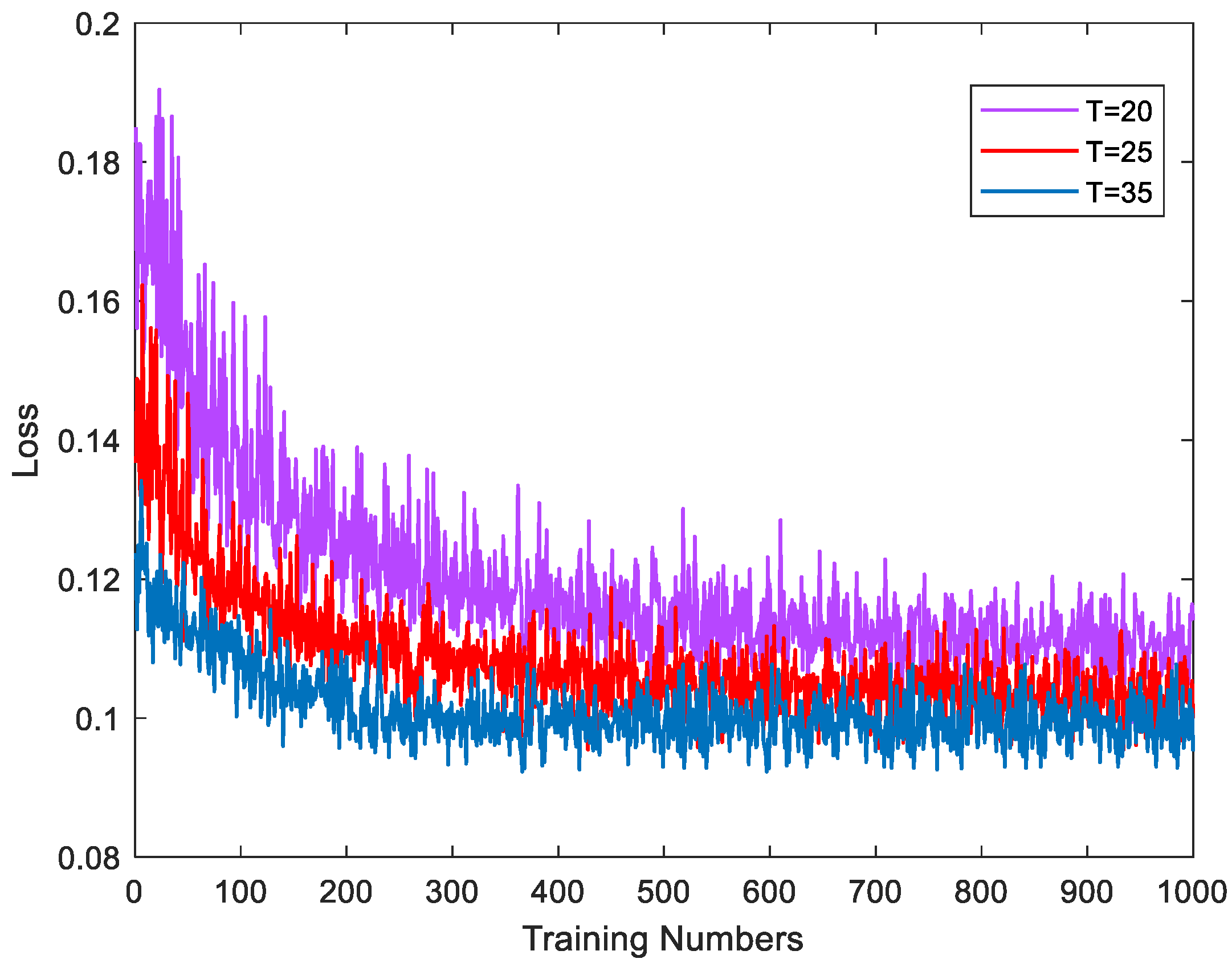
4.1. NMSE during Training

In Figure 7, we present the variation in NMSE during 1000 training iterations for networks with T = 20, T = 25, and T = 35 layers. It is evident that as the number of training iterations increases, the NMSE gradually decreases, ensuring the convergence of the network. As the number of network layers increases, while the computational complexity grows, there is no significant enhancement in clutter suppression performance. Therefore, in the subsequent comparative experiments, we set the number of layers for the DUGLSR-BSTAP-Net to 35 due to its acceptable convergency speed and computational complexity.

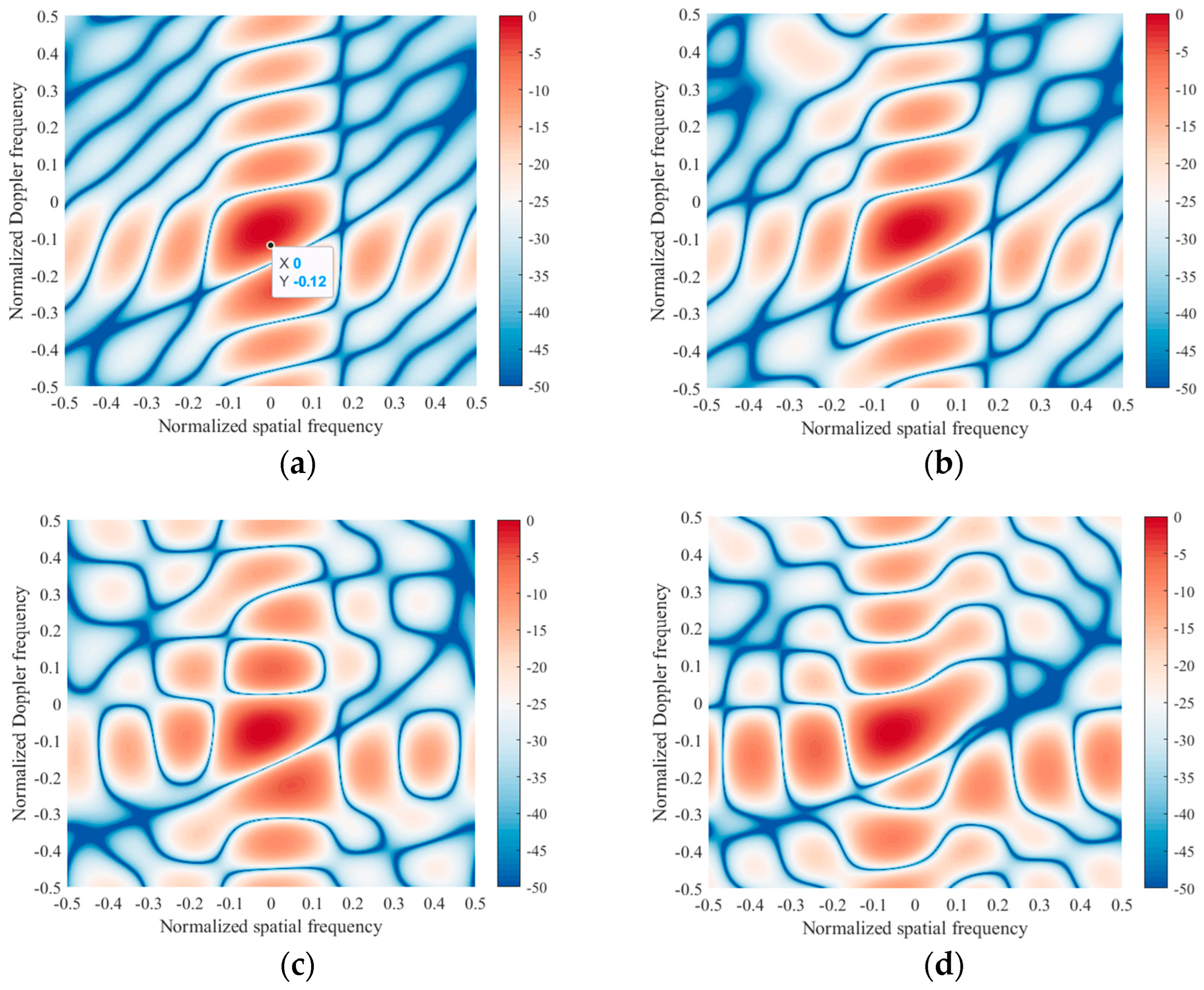
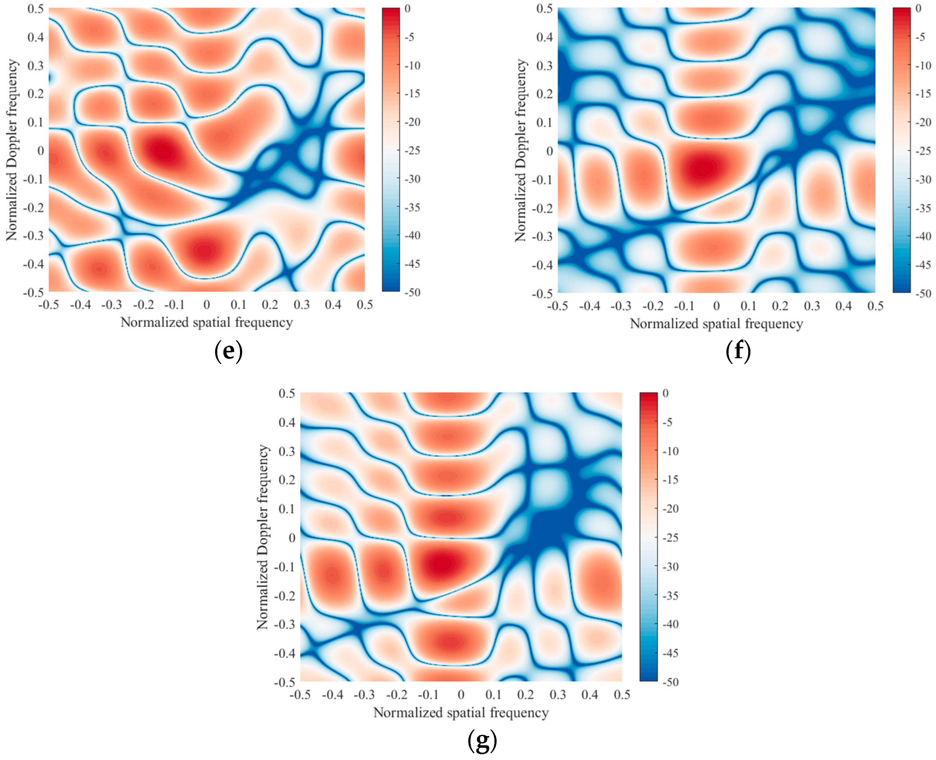
4.2. Recovered Capon Spectrum

Figure 8 illustrates the comparison of clutter Capon spectrum recovery effects under the configuration of two aircraft flying in a collinear formation $(c_T=(150\mathrm{KM},0,8\mathrm{KM}),c_R=(0,0,8\mathrm{KM})$$,{\alpha }_T=0°,{\beta }_T=0°,{\alpha }_R=0°,{\beta }_R=0°)$ using different methods. It is apparent that the clutter distribution in airborne bistatic configurations is more complex compared to monostatic configurations, leading to severe grid mismatch issues. This causes grid-based sparse recovery methods to struggle with accurately estimating the CNCM. To ensure a fair comparison, we also iterate the ANM algorithm 35 times, setting the parameters to ${\lambda }_{\mathcal{A}}=0.5$ and $\rho =0.01$, identical to the initial setting for DUGLSR-BSTAP-Net.

4.3. Adaptive Pattern

To further elucidate the performance of the DUGLSR-BSTAP-Net, we present the adaptive patterns generated by various algorithms in this part, conducted under the condition of two aircraft flying in a collinear formation $(c_T=(150\mathrm{KM},0,8\mathrm{KM}),c_R=(0,0,8\mathrm{KM}),$${\alpha }_T=0°,{\beta }_T=0°,{\alpha }_R=0°,{\beta }_R=0°)$. In this scenario, we assumed the target to be situated at a normalized spatial frequency of 0 with a normalized Doppler frequency of −0.12. The results, depicted in Figure 9, demonstrate that the proposed algorithm effectively maintains the high gain of the target while simultaneously creating a notch at the clutter ridge. This results in the suppression of both main lobe and sidelobe clutter. In contrast, the MFOCUSS and MOMP algorithms fail to accurately form the notch at the clutter ridge, leading to distorted adaptive patterns Figure 9.

4.4. Comparison of Eigenspectra

The eigenspectra of optimum CNCM and estimated CNCM are shown in Figure 10. It is evident that the eigenspectra decline progressively in both algorithms. Figure 10 also demonstrates that the large eigenvalues of the CNCM eigenspectra estimated by our proposed algorithm are the closest to those of the ideal covariance matrix. Since the large eigenvalues represent the clutter components, it can be said that the clutter subspace estimated by the proposed algorithm is the more accurate compared to other algorithms.

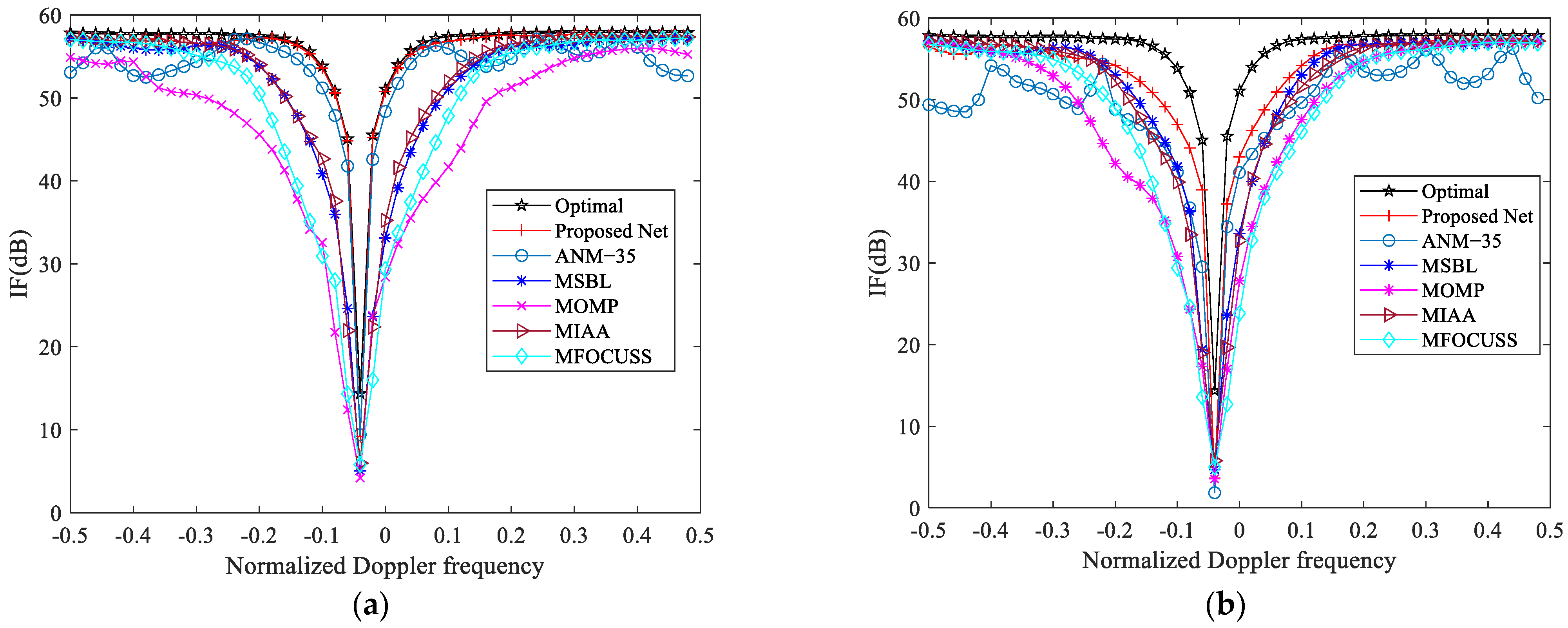
4.5. IF of Different Algorithms

In this subsection, we present comparative improvement factor curves of various algorithms under ideal condition and with array Gain-phase (Gp) error (set to ±0.05, ±2°) to evaluate the clutter suppression performance. Figure 11a shows that, due to severe grid mismatch issues under bistatic conditions, the performance of grid-based sparse recovery algorithms significantly deteriorates, resulting in wider nulls that fail to maintain target direction gain effectively. Additionally, the gridless ANM algorithm, with only 35 iterations, does not perform as well in clutter suppression compared to our proposed DUGLSR-BSTAP-Net algorithm. Therefore, we can conclude that the data-driven deep neural network approach overcomes some of the shortcomings of traditional iterative models. From Figure 11b, we can see that when the Gp error is present, the performance of the ANM algorithm deteriorates significantly, whereas the DUGLSR-BSTAP-Net experiences less performance loss. This indicates that the trained network is more robust compared to traditional algorithms, mitigating the sensitivity to errors that was a drawback in the original algorithms.

As shown in the above figure, we already observed the comparison of the improvement factor (IF) when the number of iterations for the ANM algorithm is the same as the number of layers in the DUGLSR-BSTAP-Net. Next, we will perform more iterations of the ANM algorithm to compare the clutter suppression performance.

From Figure 12a, we can see that, in an ideal case, 150 iterations of the ANM algorithm achieve the same clutter suppression performance as the 35-layer DUGLSR-BSTAP-Net. However, when the Gp error is present in Figure 12b, even after 150 iterations, the ANM algorithm still exhibits a slight performance gap compared to the proposed network. This indicates that the trained network can achieve a better performance with lower computational complexity, regardless of whether Gp error is present.

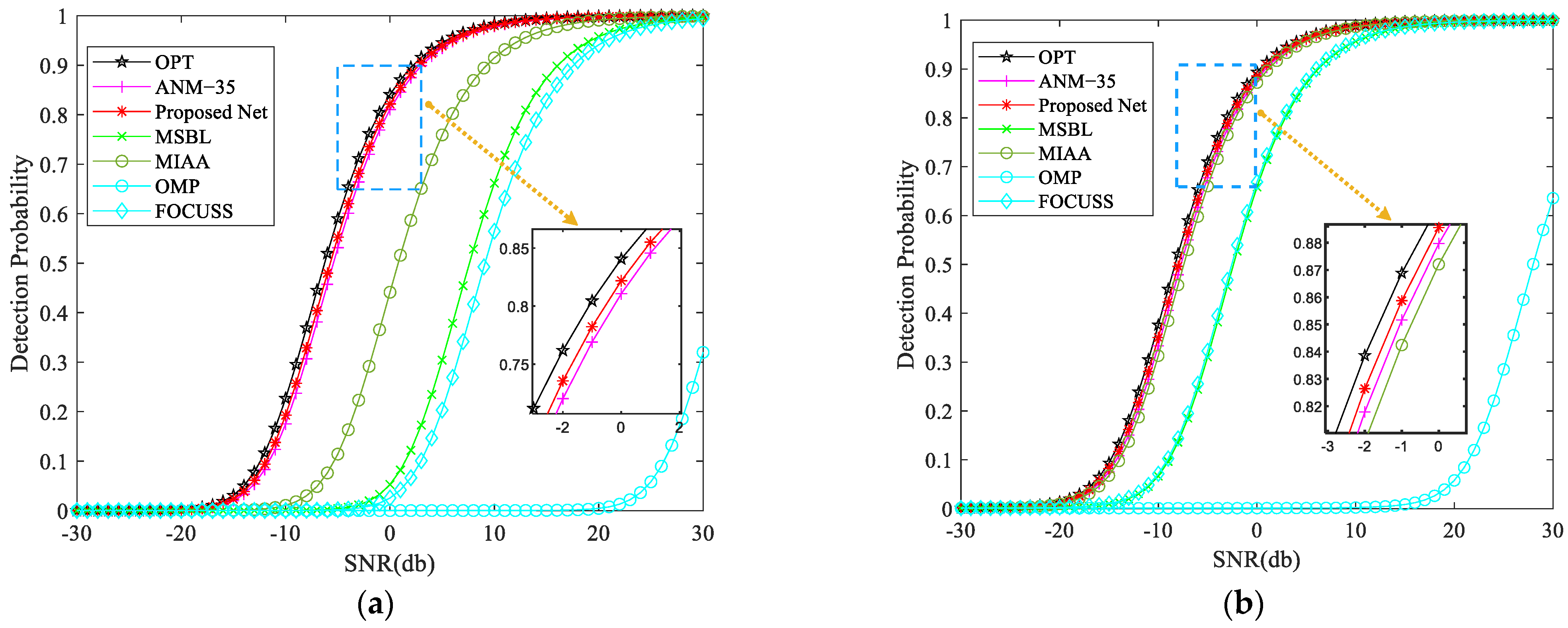
4.6. Target Detection Probability under Different SNR

The ultimate goal of STAP is to achieve target detection. Therefore, after comparing clutter suppression performance, we need to compare how the target detection probability of different algorithms varies with signal-to-noise ratio (SNR) under constant false alarm rate condition. The false alarm probability is fixed to ${10}^{-4}$. In Figure 13a,b, we compare the target detection probability of different algorithms with a slow-moving target (normalized Doppler frequency of 0.08) and a fast-moving target (normalized Doppler frequency of 0.25) added to the CUT in an ideal case, respectively. The results indicate that in an airborne bistatic radar system, the DUGLSR-BSTAP-Net and ANM algorithm exhibits better target detection performance compared to grid-based SR-STAP.

In Figure 14a,b, we compare the target detection probability of different algorithms with a slow-moving target (normalized Doppler frequency of 0.08) and a fast-moving target (normalized Doppler frequency of 0.2) added to the CUT in the non-ideal case, respectively. When the GP error is present, the target detection performance of the ANM algorithm deteriorates significantly. However, the DUGLSR-BSTAP-Net algorithm maintains the performance closest to that of the optimal filter in detecting both slow-moving and fast-moving targets.

4.7. Computational Efficiency

In this experiment, we assess the computational efficiency of various algorithms by measuring their average running time in

Table 2. Average running time.

Algorithm	Time	Unit
ANM-35	0.283	s
ANM-150	0.847	s
MSBL	14.425	s
MIAA	2.100	s
MOMP	0.025	s
MFOCUSS	3.687	s
DUGLSR-BSTAP-Net	0.304	s

. The simulation results for ANM-35, ANM-150, MSBL, MIAA, MOMP, and MFOCUSS were obtained using MATLAB 2022b, while the results for DUGLSR-BSTAP-Net were obtained using Python 3.8 and PyTorch 1.8. Both were installed on a computer equipped with an AMD Ryzen 7 5800H processor with Radeon Graphics at 3.20 GHz.

5. Conclusions

In this article, we provide a detailed derivation of the signal model for airborne bistatic clutter and unfolding ANM into a deep neural network. After extensive data training, the initially suboptimal model parameters were corrected, enhancing the clutter suppression performance. Each layer of the network contains five sub-layers, each with its own physical meaning, thereby improving the interpretability of the network. The simulation results demonstrate that the proposed algorithm achieves excellent clutter suppression and target detection performance.

References

1. Brennan, L.E.; Reed, L.S. Theory of Adaptive Radar. IEEE Trans. Aerosp. Electron. Syst. 1973, AES-9, 237–252. [Google Scholar] [CrossRef]
2. Klemm, R. Principles of Space-Time Adaptive Processing. In Radar, Sonar and Navigation; John Wiley & Sons, Inc.: Hoboken, NJ, USA, 2006. [Google Scholar]
3. Melvin, W.L. Chapter 12—Space-Time Adaptive Processing for Radar. In Academic Press Library in Signal Processing; Sidiropoulos, N.D., Gini, F., Chellappa, R., Theodoridis, S., Eds.; Elsevier: Amsterdam, The Netherlands, 2014; Volume 2, pp. 595–665. ISBN 9780123965004. ISSN 2351-9819. [Google Scholar] [CrossRef]
4. Ward, J. Space-time adaptive processing for airborne radar. In Proceedings of the 1995 International Conference on Acoustics, Speech, and Signal Processing, Detroit, MI, USA, 9–12 May 1995. [Google Scholar]
5. Reed, I.S.; Mallett, J.D.; Brennan, L.E. Rapid Convergence Rate in Adaptive Arrays. IEEE Trans. Aerosp. Electron. Syst. 1974, AES-10, 853–863. [Google Scholar] [CrossRef]
6. Maria, S.; Fuchs, J.-J. Application of the Global Matched Filter to Stap Data an Efficient Algorithmic Approach. In Proceedings of the 2006 IEEE International Conference on Acoustics Speech and Signal Processing Proceedings, Toulouse, France, 14–19 May 2006; p. 4. [Google Scholar] [CrossRef]
7. Sun, K.; Zhang, H.; Li, G.; Meng, H.; Wang, X. A novel STAP algorithm using sparse recovery technique. In Proceedings of the 2009 IEEE International Geoscience and Remote Sensing Symposium, Cape Town, South Africa, 12–17 July 2009; pp. V-336–V-339. [Google Scholar] [CrossRef]
8. Sun, K.; Meng, H.; Wang, Y.; Wang, X. Direct data domain STAP using sparse representation of clutter spectrum. Signal Process. 2011, 91, 2222–2236. [Google Scholar] [CrossRef]
9. Yang, Z.; Li, X.; Wang, H.; Jiang, W. Adaptive clutter suppression based on iterative adaptive approach for airborne radar. Signal Process. 2013, 93, 3567–3577. [Google Scholar] [CrossRef]
10. Yang, Z.; Li, X.; Wang, H.; Jiang, W. On Clutter Sparsity Analysis in Space–Time Adaptive Processing Airborne Radar. IEEE Geosci. Remote Sens. Lett. 2013, 10, 1214–1218. [Google Scholar] [CrossRef]
11. Duan, K.; Wang, Z.; Xie, W.; Chen, H.; Wang, Y. Sparsity-based stap algorithm with multiple measurement vectors via sparse bayesian learning strategy for airborne radar. IET Signal Process. 2017, 11, 544–553. [Google Scholar] [CrossRef]
12. Liu, C.; Wang, T.; Zhang, S.; Ren, B. Clutter suppression based on iterative reweighted methods with multiple measurement vectors for airborne radar. IET Radar Sonar Navig. 2022, 16, 1446–1459. [Google Scholar] [CrossRef]
13. Cui, W.; Wang, T.; Wang, D.; Liu, C. An Improved Iterative Reweighted STAP Algorithm for Airborne Radar. Remote Sens. 2023, 15, 130. [Google Scholar] [CrossRef]
14. Candès, E.J.; Fernandez-Granda, C. Towards a mathematical theory of super-resolution. Commun. Pure Appl. Math. 2014, 67, 906–956. [Google Scholar] [CrossRef]
15. Tang, G.; Bhaskar, B.N.; Shah, P.; Recht, B. Compressed Sensing Off the Grid. IEEE Trans. Inf. Theory 2013, 59, 7465–7490. [Google Scholar] [CrossRef]
16. Feng, W.; Guo, Y.; Zhang, Y.; Gong, J. Airborne radar space time adaptive processing based on atomic norm minimization. Signal Process. 2018, 148, 31–40. [Google Scholar] [CrossRef]
17. Zhang, T.; Hu, Y.; Lai, R. Gridless super-resolution sparse recovery for non-sidelooking STAP using reweighted atomic norm minimization. Multidimens. Syst. Signal Process. 2021, 32, 1259–1276. [Google Scholar] [CrossRef]
18. Li, Z.; Wang, T.; Su, Y. A fast and gridless stap algorithm based on mixed-norm minimisation and the alternating direction method of multipliers. IET Radar Sonar Navig. 2021, 15, 1340–1352. [Google Scholar] [CrossRef]
19. Cui, W.; Wang, T.; Wang, D.; Zhang, X. A novel sparse recovery-based space-time adaptive processing algorithm based on gridless sparse Bayesian learning for non-sidelooking airborne radar. IET Radar Sonar Navig. 2023, 17, 1380–1390. [Google Scholar] [CrossRef]
20. Duan, K.; Chen, H.; Xie, W.; Wang, Y. Deep learning for high-resolution estimation of clutter angle-Doppler spectrum in STAP. IET Radar Sonar Navig. 2022, 16, 193–207. [Google Scholar] [CrossRef]
21. Zou, B.; Wang, X.; Feng, W.; Lu, F.; Zhu, H. Memory-Augmented Autoencoder-Based Nonhomogeneous Detector for Airborne Radar Space-Time Adaptive Processing. IEEE Geosci. Remote Sens. Lett. 2024, 21, 3502405. [Google Scholar] [CrossRef]
22. Zhu, H.; Feng, W.; Feng, C.; Zou, B.; Lu, F. Deep unfolding based space-time adaptive processing method for airborne radar. J. Radars 2022, 11, 676–691. [Google Scholar] [CrossRef]
23. Li, Y.; Chi, Y. Off-the-Grid Line Spectrum Denoising and Estimation with Multiple Measurement Vectors. IEEE Trans. Signal Process. 2016, 64, 1257–1269. [Google Scholar] [CrossRef]
24. Boyd, S.; Parikh, N.; Chu, E.; Peleato, B.; Eckstein, J. Distributed Optimization and Statistical Learning via the Alternating Direction Method of Multipliers; Foundations and Trends® in Machine Learning: Hanover, MA, USA, 2011. [Google Scholar] [CrossRef]
25. He, K.; Zhang, X.; Ren, S.; Sun, J. Deep Residual Learning for Image Recognition. In Proceedings of the 2016 IEEE Conference on Computer Vision and Pattern Recognition (CVPR), Las Vegas, NV, USA, 27–30 June 2016; pp. 770–778. [Google Scholar] [CrossRef]
26. Kingma, D.P.; Ba, J. Adam: A method for stochastic optimization. arXiv 2014, arXiv:1412.6980. [Google Scholar]
27. Pati, Y.C.; Rezaiifar, R.; Krishnaprasad, P.S. Orthogonal matching pursuit: Recursive function approximation with applications to wavelet decomposition. In Proceedings of the 27th Asilomar Conference on Signals, Systems and Computers, Pacific Grove, CA, USA, 1–3 November 1993; IEEE: Piscataway, NJ, USA, 1993; pp. 40–44. [Google Scholar]
28. Gorodnitsky, I.F.; Rao, B.D. Sparse signal reconstruction from limited data using FOCUSS: A re-weighted minimum norm algorithm. IEEE Trans. Signal Process. 1997, 45, 600–616. [Google Scholar] [CrossRef]
29. Li, Z.; Wang, T. ADMM-Based Low-Complexity Off-Grid Space-Time Adaptive Processing Methods. IEEE Access 2020, 8, 206646–206658. [Google Scholar] [CrossRef]
Figure 1. Geometric configuration of airborne bistatic radar system.
Remotesensing 16 02516 g001
Figure 2. Bistatic constant range ellipsoids. (a) Before transformations. (b) After transformations.
Remotesensing 16 02516 g002
Figure 3. The clutter ridge distributions for four different bistatic configurations: (a) transmitter and receiver fly in parallel; (b) transmitter and receiver fly collinearly; (c) transmitter and receiver fly in a cross pattern; and (d) transmitter and receiver fly perpendicularly.
Remotesensing 16 02516 g003
Figure 4. A clear depiction of the deep unfolding.
Remotesensing 16 02516 g004
Figure 5. An example of DUGLSR-BSTAP-Net with three layers.
Remotesensing 16 02516 g005
Figure 6. The data flow graph of DUGLSR-BSTAP-Net.
Remotesensing 16 02516 g006
Figure 7. Training loss of different network depth.
Remotesensing 16 02516 g007
Figure 8. Comparison of the recovered capon spectrum. (a) optimal; (b) proposed net (DUGLSR−BSTAP−Net); (c) ANM−35; (d) MSBL; (e) MOMP; (f) MIAA; (g) MFOCUSS.
Remotesensing 16 02516 g008
Figure 9. Comparison of adaptive pattern. (a) Optimal; (b) Proposed Net (DUGLSR−BSTAP−Net); (c) ANM−35; (d) MSBL; (e) MOMP; (f) MIAA; and (g) MFOCUSS.
Remotesensing 16 02516 g009aRemotesensing 16 02516 g009b
Figure 10. CNCM eigenspectra estimated by different algorithms under two aircraft flying in a collinear formation.
Remotesensing 16 02516 g010
Figure 11. Comparison results of IF under bistatic collinear configuration, which is the same as in Section 4.2. (a) Ideal case; and (b) With GP error (±0.05, ±2°).
Remotesensing 16 02516 g011
Figure 12. Comparison of the clutter performance between ANM with different iteration counts and proposed net (DUGLSR−BSTAP−Net). (a) Ideal case. (b) With GP error (±0.05, ±2°).
Remotesensing 16 02516 g012
Figure 13. Comparison of target detection performance in ideal case. (a) Slow-moving target. (b) Fast-moving target.
Remotesensing 16 02516 g013
Figure 14. Comparison of target detection performance with GP-error (±0.05, ±2°). (a) Slow-moving target. (b) Fast-moving target.
Remotesensing 16 02516 g014