Article

Data Matters: Rethinking the Data Distribution in Semi-Supervised Oriented SAR Ship Detection

by
Yimin Yang
1,
Ping Lang
1,
Junjun Yin
2,
Yaomin He
3 and
Jian Yang
1,*
1
Department of Electronic Engineering, Tsinghua University, Beijing 100084, China
2
School of Computer and Communication Engineering, University of Science and Technology, Beijing 100083, China
3
Institute of Systems Engineering, Academy of Military Sciences, People’s Liberation Army of China, Beijing 100071, China
*
Author to whom correspondence should be addressed.
Remote Sens. 2024, 16(14), 2551; https://doi.org/10.3390/rs16142551
Submission received: 22 May 2024 / Revised: 3 July 2024 / Accepted: 9 July 2024 / Published: 11 July 2024

Abstract

:
Data, in deep learning (DL), are crucial to detect ships in synthetic aperture radar (SAR) images. However, SAR image annotation limitations hinder DL-based SAR ship detection. A novel data-selection method and teacher–student model are proposed in this paper to effectively leverage sparse labeled data and improve SAR ship detection performance, based on the semi-supervised oriented object-detection (SOOD) framework. More specifically, we firstly propose a SAR data-scoring method based on fuzzy comprehensive evaluation (FCE), and discuss the relationship between the score distribution of labeled data and detection performance. A refined data selector (RDS) is then designed to adaptively obtain reasonable data for model training without any labeling information. Lastly, a Gaussian Wasserstein distance (GWD) and an orientation-angle deviation weighting (ODW) loss are introduced to mitigate the impact of strong scattering points on bounding box regression and dynamically adjusting the consistency of pseudo-label prediction pairs during the model training process, respectively. The experiments results on four open datasets have demonstrated that our proposed method can achieve better SAR ship detection performances on low-proportion labeled datasets, compared to some existing methods. Therefore, our proposed method can effectively and efficiently reduce the burden of SAR ship data labeling and improve detection capacities as much as possible.

1. Introduction

Synthetic aperture radar (SAR) is a type of active radar that can image the surface of the sea and ground. Compared to optical remote sensing, SAR has the unique advantages of being able to perform high-quality surface imaging all-weather and all-day, having important application values in marine surveillance, resource census, disaster monitoring, and other fields.
As one of the important applications, the detection of ship targets in SAR images is of great value in both the military and civilian fields [1]. With the development of deep learning (DL), the performance of ship detection in SAR images has been significantly improved [2]. However, there are many bottlenecks in the existing DL-based SAR ship detectors in real applications:
i.
A dataset with complex scenarios can improve the generalization ability of the trained model, but currently, there are only a few indicators to qualitatively judge the complexity of data, such as nearshore and offshore, and there are no indicators that can be quantified.
ii.
The training process of DL models requires diverse and a large amount of labeled data. However, labeling ship targets in SAR images is time-consuming and expensive.
iii.
The traditional horizontal bounding box (HBB)-labeling method has difficulty describing the complex shapes and diverse directions of ship targets, and the HBB-labeling method often results in a large overlap area when ships are densely berthed near the shore, as shown in Figure 1a.
iv.
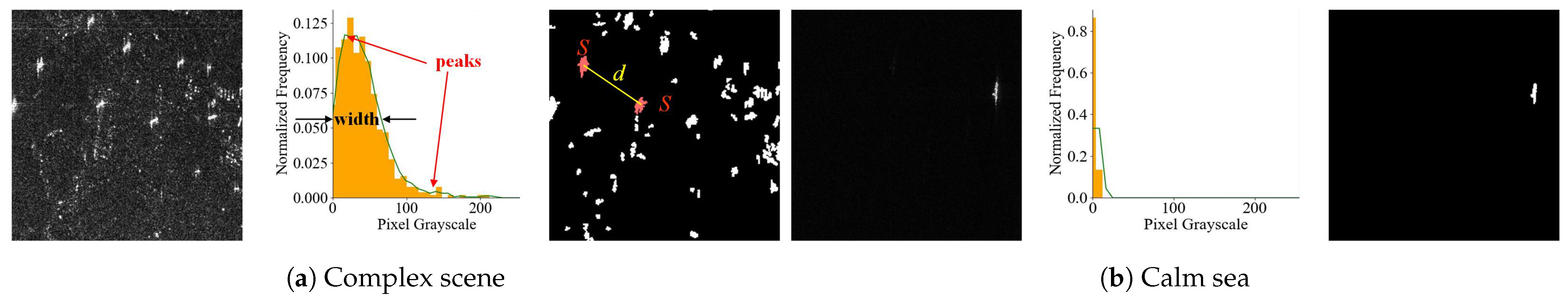
As shown in Figure 1b, there is much unavoidable speckle noise, strong sea clutter, and high sidelobe levels, caused by strong scattering points in SAR images, which increases the difficulty of detection to some extent.
Figure 1. (a) Annotation results of oriented bounding box (OBB) and horizontal bounding box (HBB). (b) Some difficulties in labeling ship targets in SAR images: high sidelobe levels, strong sea clutter, and interference.
Remotesensing 16 02551 g001
To address aforementioned issues, we propose some solutions as follows: For problem i, considering that the evaluation of whether the scene of a SAR image is complex or not is fuzzy, we selected the statistical characteristics of the gray-scale image, such as the mean value and variance, combined with simple morphology processing to obtain the spatial characteristics as indicators and used fuzzy comprehensive evaluation (FCE) [3] to score them. For problem ii, on the one hand, when creating datasets, using appropriate methods to select a small number of SAR image slices can reduce the burden of manual annotation without affecting the training. On the other hand, semi-supervised learning can combine a small amount of labeled data and a large amount of unlabeled data to improve the model performance and robustness of ship detection. For problem iii, the oriented bounding box (OBB)-labeling method can more accurately describe the ship’s morphological characteristics and provide course information, which is helpful for track prediction. For problem iv, the Gaussian Wasserstein distance (GWD) [4] loss can effectively reduce the inconsistency between the loss function and the metric in oriented object detection and can basically alleviate the influence of strong scattering points on ship edge identification.
This paper focuses on the distribution of labeled data and the semi-supervised oriented object-detection algorithm. The overview of our proposed method is shown in Figure 2. Our main contributions are summarized as follows:
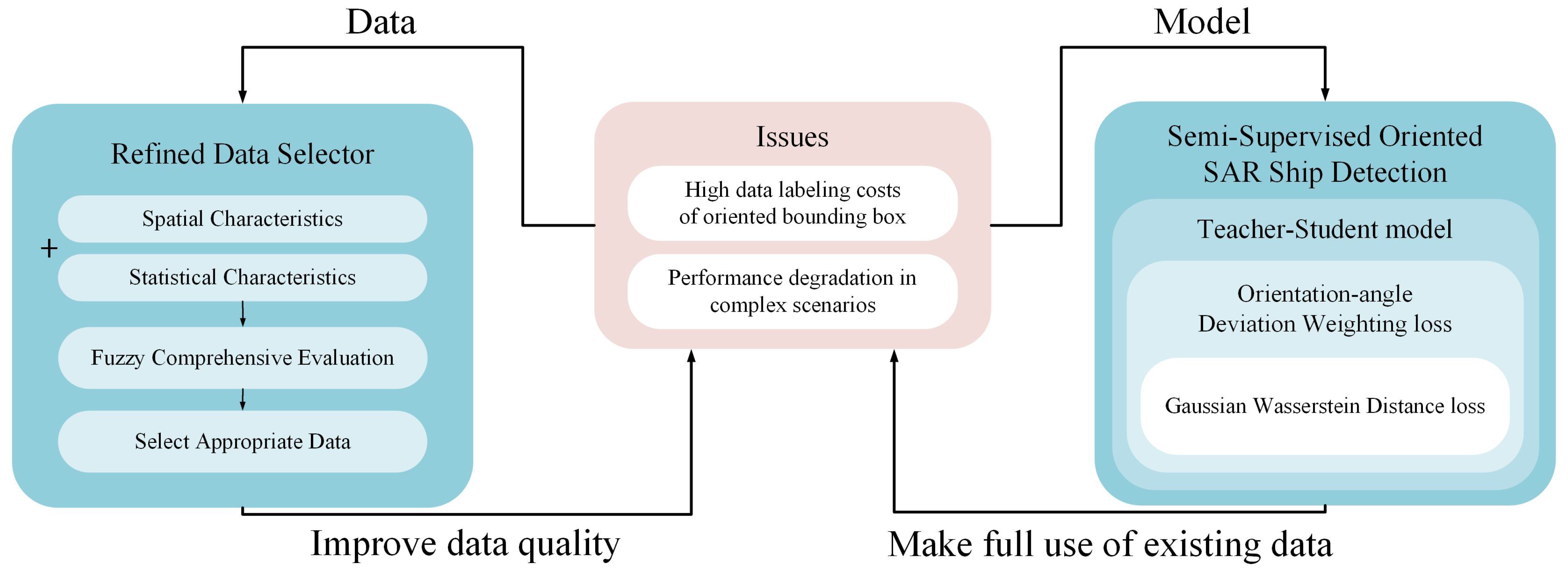
  • We propose a novel framework based on a semi-supervised oriented object-detection (SOOD) [5] model according to the characteristics of the SAR ship-detection task. An orientation-angle deviation weighting (ODW) loss is proposed, which uses the GWD loss for bounding box regression.
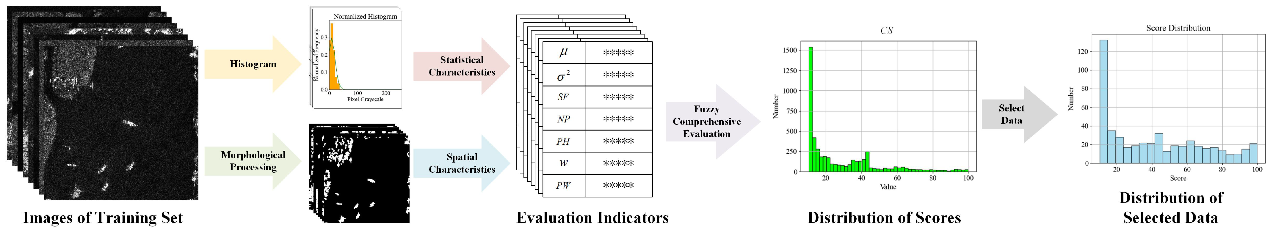
  • We propose a data-scoring mechanism based on FCE. According to the statistical characteristics of the data pixel gray-scale values and their spatial characteristics after graphics processing, a reasonable membership function is set, and each picture in the dataset is scored by FCE. Finally, the comprehensive scores of the data that are similar to the intuition are obtained.
  • We propose a refined data selector (RDS) to select data with an appropriate score distribution. With the same amount of labeled data, the RDS can improve the training performance of the semi-supervised training algorithm model as much as possible. Therefore, when generating a new dataset of SAR ship detection data, the proposed method can be used to pre-select the data slices, which can reduce the burden of labeling and obtain data with more abundant scenes.
The remainder of this article is organized as follows. Section 2 discusses related works on SAR ship detection and semi-supervised object detection. Section 3 introduces the proposed methods for oriented semi-supervised SAR ship detection and the refined data selector. Section 4 introduces the datasets and experimental results and analysis. Section 5 summarizes this study.

2. Related Works

At present, many achievements have been made in the field of SAR ship detection and addressing labeling costs: SAR ship detection mainly uses constant false alarm rate (CFAR) detection and DL-based object detection, and the labeling costs are mainly addressed using semi-supervised object detection.

2.1. SAR Ship Detection

CFAR is a classic target-detection algorithm in the field of radar. The CFAR detection method dynamically adjusts the detection threshold according to the statistical characteristics of radar echo data to keep the radar false alarm rate constant. This classical method is also widely used in the detection of ship targets in SAR images. This method largely depends on the statistical modeling of sea clutter and the parameter estimation of the chosen model. Commonly used distributions include the Gamma distribution, the log-normal distribution, the Weibull distribution, and the K distribution [1].
There are many improvements to the CFAR, among which superpixel-segmentation-based methods are mainstream: first, the SAR image is segmented into superpixels, and then, CFAR detection is performed at the superpixel level. This method can improve detection speed and performance in high-resolution SAR images [6,7,8,9,10,11]. Using polarimetric information for target detection is also a very important direction. Single-polarization SAR can only acquire information on the backscattering intensity of ground objects, whereas polarimetric synthetic aperture radar (PolSAR) can obtain the complete scattering characteristics of targets. By leveraging the differences in scattering characteristics between ships and sea clutter, PolSAR can effectively distinguish between them and perform ship detection through polarimetric channel synthesis, polarimetric optimization, and scattering mechanisms [12,13,14,15,16]. In addition, there are methods based on modeling sea clutter using new distributions such as the α -stable distribution and log-normal mixture models [17,18,19], and Refs. [20,21] used the automatic identification system (AIS) to assist CFAR detection.
However, the performance is poor in complex scenarios such as strong clutter, nearshore targets, and multiple targets. Additionally, CFAR detection suffers from low computational efficiency and poor transferability.
DL has become the mainstream research direction for ship detection in SAR images. DL-based SAR ship-detection methods can be categorized into anchor-based and anchor-free classes, depending on whether the network model uses preset anchor boxes. Anchor-based methods can further be divided into single-stage and two-stage methods, depending on whether the network model needs to generate proposed regions.
There are many DL-based methods for SAR ship detection. Since the size of anchor boxes needs to be manually adjusted or set based on the clustering of the training dataset, these fixed anchor boxes are not always suitable for other datasets with different distributions. Additionally, to ensure a high recall rate, a large number of anchor boxes needs to be set, which introduces significant computational overhead in SAR ship detection where targets are relatively sparse. Therefore, studies [22,23,24] have adopted anchor-free structures. Transformers capture dependencies between all positions in the input sequence through the self-attention mechanism. This means that, regardless of the distance between two elements in the sequence, Transformers can directly calculate their relationships, thereby better understanding the global context. In contrast, the convolutional neural network (CNN) achieves local perception through convolutional kernels. Although the receptive field can be extended by increasing the number of layers and using larger convolutional kernels, CNNs still tend to focus on local feature extraction and have difficulty in capturing long-range global context information. Hence, studies [24,25,26] have replaced the backbone network from CNNs to Transformers. Additionally, there are other measures to improve network models from aspects such as non-maximum suppression, using frequency domain information, and attention mechanisms [27,28,29]. DL-based methods have inherent advantages in feature extraction and offer higher robustness for different scenarios compared to traditional methods.
However, since deep learning is a data-driven detection method, it has high requirements for the dataset.

2.2. Addressing Labeling Costs

Semi-supervised learning combines supervised and unsupervised learning, making full use of a small amount of labeled data along with a large amount of unlabeled data. This approach can effectively improve the model’s generalization ability across different scenarios.
The pseudo-label method is a mainstream approach in semi-supervised object detection. Pseudo-label methods predict the pseudo-labels for unlabeled images by using a pretrained model and then jointly train the model with both labeled and unlabeled data after augmentation. Self-training uses labeled data to train a high-quality teacher model, which is used to predict the unlabeled data and, finally, uses all the data to train a student model [30,31]. Currently, mainstream pseudo-label-based semi-supervised learning methods for object detection use the Mean Teacher approach. In the unsupervised learning part, the teacher model generates pseudo-labels for the unlabeled data, which are then used by the student model. The teacher model is updated using the exponential moving average (EMA), so end-to-end training can be performed. During this process, the quality of the pseudo-labels generated by the teacher model is crucial. Consequently, many methods focus on improving the accuracy of the pseudo-labels through techniques such as dense pseudo-labeling, pixel-level prediction, and a soft threshold [32,33,34,35,36,37]. The aforementioned semi-supervised learning models are all designed for general object-detection tasks using horizontal bounding boxes (HBBs). SOOD [5] is the first semi-supervised object-detection algorithm specifically proposed for oriented object detection in remote sensing images.
However, the blurred ship edges and speckle noise in SAR images can have a significantly adverse impact on detection performance.
In addition, weakly supervised learning, few-shot learning, and active learning also help address labeling costs. Unlike other methods that alleviate the problem from an algorithmic perspective, active learning addresses the issue from a data perspective. Active learning aims to maximize the training performance of the model while minimizing the amount of labeling required. In other words, it seeks to select the fewest, but most useful samples from the unlabeled data for experts to label, thereby reducing labeling costs while maintaining training effectiveness [38,39,40]. Active learning methods are also applied to SAR image recognition [41,42,43], and the results, after further labeling, can also serve as datasets for object detection.
Using model training methods for SAR data selection may be overly complex and unnecessary. Optical images possess rich texture details and colors, making it difficult to describe an optical image using simple indicators such as the mean and variance. In contrast, SAR images typically appear as gray-scale images with fewer texture details, allowing for data selection using non-learning and simpler methods. In SAR ship-detection tasks, considering the gray-scale differences between ships and the sea surface, the darker areas usually represent the sea surface, while the brighter areas represent ships, interference, or land clutter. Therefore, the statistical and spatial distributions of gray-scale values can effectively describe the scene and exhibit good generalization ability.

3. Methods

The research approach and methodology of this paper are shown in Figure 3. To address the issues of high data labeling costs and performance degradation in complex scenarios for SAR ship detection, this paper proposes solutions from both the data and model perspectives.
On the data side, a certain percentage of training data is selected as labeled data through the RDS, which has a good representation and includes as many scenarios as possible, to enhance the model’s training performance. First, we obtain the spatial and statistical features of SAR images as evaluation indicators, then use fuzzy comprehensive evaluation to score the images comprehensively, and finally, select the appropriate data based on the comprehensive scores.
On the model side, we designed a semi-supervised oriented SAR ship-detection framework that can fully utilize the existing labeled data and a large amount of unlabeled data. The specific process is shown in Figure 2. For the first few iterations, known as the “burn-in” stage, supervised training of the student model is performed using only labeled data, and the teacher model is updated by the exponential moving average (EMA). In the unsupervised training stage, the unsupervised loss is calculated between pseudo-label prediction pairs.
The function of each component is shown in Table 1. In practical applications, if a new SAR ship detection dataset needs to be established, the required amount of data is first selected using the refined data selector (RDS), ensuring that the scenes are highly representative. These selected images are then labeled. Subsequently, the proposed semi-supervised learning model is trained using this small amount of labeled data along with the remaining large amount of unlabeled data. This approach ensures the model’s detection performance while minimizing the labeling burden.

3.1. Refined Data Selector

Selecting an appropriate dataset is crucial in semi-supervised object detection. When using a semi-supervised object-detection method, selecting a suitable dataset can reduce the workload and cost of annotation, on the one hand, and also improve the performance of the model, on the other hand. In general, a SAR image with strong interference, strong clutter, and various scattering points must be more complex than the scene of a calm sea. Since the evaluation of the complexity of SAR images from multiple aspects is fuzzy and subjective, fuzzy comprehensive evaluation (FCE) will make the results as objective as possible and conform to humans’ subjective feelings.
FCE is a decision analysis method used to handle the uncertainty and fuzziness of information. It is commonly applied to solve complex multi-criteria decision-making problems, where there may be cross-impact and fuzziness among various indicators. FCE quantifies uncertainty and fuzziness, synthesizing information from multiple indicators to derive a comprehensive evaluation result. After the comprehensive scores ( C S s) of all SAR image data are obtained, the data with a certain score distribution are selected as the subsequent semi-supervised learning. The process of the refined data selector (RDS) is shown in Figure 4.

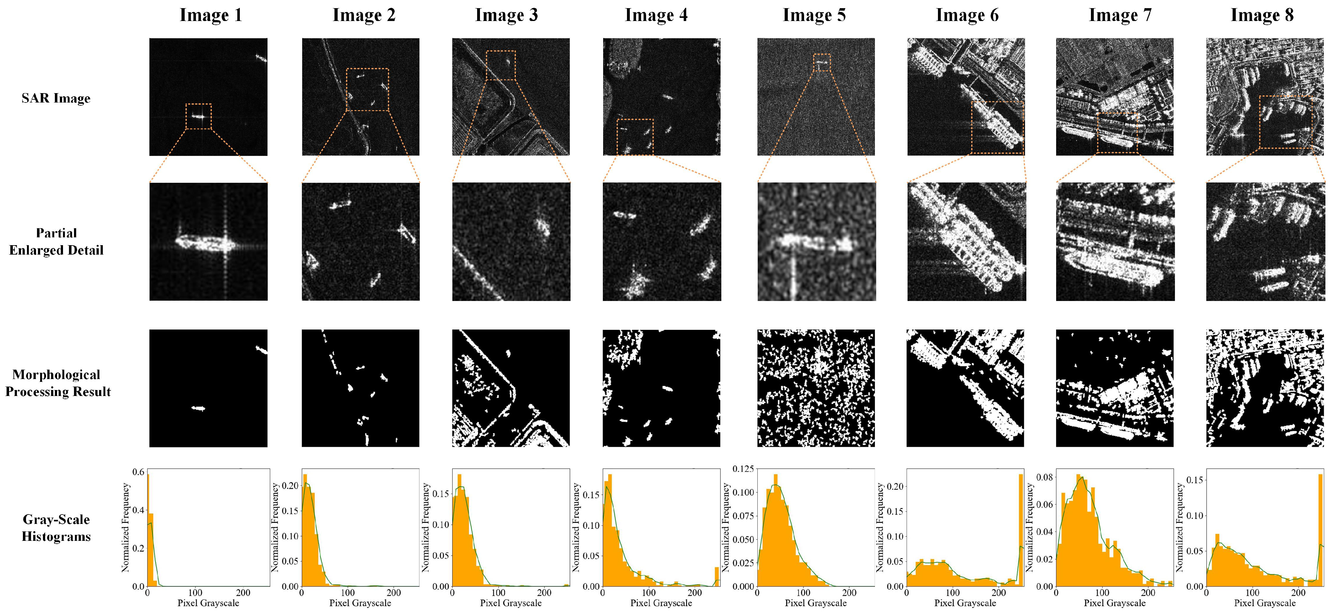
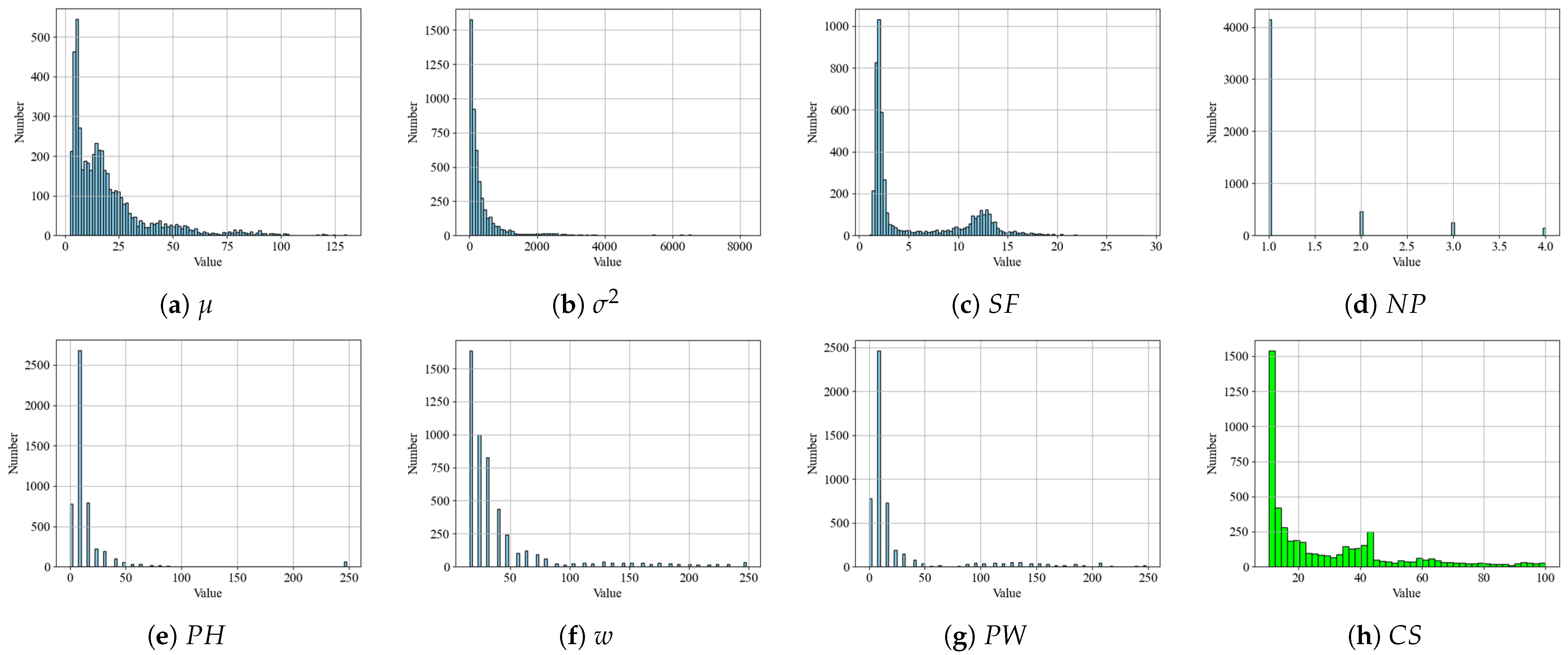
3.1.1. Construction of Evaluation Indicators

Selecting appropriate evaluation indicators in FCE is the most fundamental step. Two SAR images and their gray-scale histograms are shown in Figure 5; one is a complex scene A with strong interference, and the other is an offshore scene B with a calm sea. Obviously, the mean value and variance of Figure 5a will be significantly higher than that of Figure 5b, and it is more complex spatially. Therefore, the appropriate statistical characteristics of the gray-scale values and the spatial characteristics can be selected as the indicators of FCE. We selected 7 indicators: mean μ , variance σ 2 , spatial factor S F , number of peaks N P , position of highest peak P H , width and position of the widest peak w, and P W in the histogram. Their calculation methods are as follows.

Mean μ and Variance σ 2

The mean and variance reflect the overall intensity level of SAR images and the fluctuation level of the gray-scale values, respectively. A higher mean value means that there are more strong scattering points or a large area of strong clutter in the image, and a larger the variance means that the gray-scale value distribution in the picture is more disperse. For an image of M × N :
μ = 1 M N i = 1 M j = 1 N G ( i , j )
σ 2 = 1 M N i = 1 M j = 1 N G ( i , j ) μ 2
where G ( i , j ) represents the gray-scale value of the pixel in row i and column j.

Number of Peaks N P , Position of Highest Peak P H , Width of Widest Peak w, and Position of Widest Peak P W

The histogram analysis of SAR images reveals key characteristics for identifying ship targets and clutter. In the same SAR image, the gray-scale value of the ship target is relatively strong and uniform, and the proportion of pixels is small, so it should be displayed as a peak with a higher gray-scale value, narrower width, and lower height on the histogram. Therefore, the more peaks there are, the wider the width of the widest peak, indicating that there may be strong sea clutter, interference, or land clutter in the SAR image. Conversely, the highest peak and widest peak of SAR images with calm sea are more likely to have a lower gray-scale value, and the width is narrower, as shown in Figure 5b. The histogram of SAR image gray-scale values is drawn and smoothed. The gradient is used to identify peak values. When the gradient of the signal exceeds a certain threshold, it is considered as a peak, and the full-width at half-maximum is used to calculate the width of the peak, as shown in the middle image of Figure 5a.

Spatial Factor S F

Spatial factors reflect the spatial characteristics of SAR images and can explain the complexity of the scene to some extent. First, Otsu’s method is used to binarize SAR images and convert them to black and white. Next, we used the connected components labeling algorithm to label the connected regions in the image and obtain some statistics about each connected region, such as the area and centroid position. Then, according to the default threshold, we removed the small connected regions, which may be noise or unimportant parts. Next, we processed the binary image using the dilation operation so that adjacent white areas can be connected together, and N r regions remain. We then used a KD tree to find the nearest neighbor regions between the connected regions in the image and calculated the distance between them.
We believe that the more connected regions there are, the larger their area, and the closer the distance between adjacent regions, the larger the spatial factor is. Finally, we calculated the initial density of each pair of adjacent regions based on the distance d and the area S of connected regions, shown in Figure 5a, and obtained the final spatial factor by:
S F = 1 + k N N r 1 N r i = 1 N r ( 1 + k S S 1 + S 2 2 ) ( 1 + k d exp ( d ) )
where k N , k S , and k d denote the weights of the number, area, and distance of the connection regions, which were empirically set as 0.3, 0.05, and 0.1, respectively.

3.1.2. Fuzzy Comprehensive Evaluation

The basic process of FCE is as follows: first, determine the evaluation set and the weights of the evaluation indicators for the SAR images, ranging from simple to complex. Next, conduct corresponding fuzzy evaluations for each indicator, and determine the membership function. Then, form the fuzzy judgment matrix. Finally, perform fuzzy operations with the weight matrix to obtain a quantitative comprehensive evaluation result.

Factor Set and Evaluation Set

The seven indicators mentioned in Section 3.1.1 were set as the factor set by:
U = { μ , σ 2 , S F , N P , P H , w , P W }
Four levels were set as the evaluation set, which were used to describe the complexity of the picture:
V = { Very Simple , Simple , Complex , Very Complex }
In FCE, the weights of different evaluation indicators are crucial as they reflect the importance or role of each factor in the comprehensive decision-making process, directly affecting the outcome. S F is the only spatial feature that can adequately reflect the spatial distribution of pixels in SAR images, thereby indicating the complexity of the scene. Therefore, we assigned it the highest weight. μ , σ 2 , and w can fully reflect the overall intensity distribution of SAR images, so they are given moderate weights. For histograms with a single peak, N P , P H , and P W cannot independently reflect the scene complexity of SAR images; hence, they are assigned lower weights. Based on this, by fine-tuning these weights, we found that the final evaluation aligns better with our intuitive understanding of SAR image scene complexity when the weight vector is A = ( 0.15 , 0.2 , 0.25 , 0.05 , 0.1 , 0.15 , 0.1 ) . In addition, the entropy weight method and the analytic hierarchy process can be used to determine the weights. Although the empirically assigned weights used in this paper are somewhat subjective, they reflect the actual situation to a certain extent, and the final evaluation results are relatively accurate.

Comprehensive Evaluation Matrix

Construct the comprehensive evaluation matrix R and perform the comprehensive evaluation in conjunction with the weights A.
R = r 11 r 12 r 14 r 21 r 22 r 24 r 71 r 72 r 74 B = A R = b 1 , b 2 , b 3 , b 4
where B is the normalized fuzzy evaluation set. ∘ denotes the weighted average fuzzy product of a row vector and a matrix, expressed as:
b j = min 1 , i = 1 7 a i r i j
The weighted average principle is used to draw a comprehensive conclusion and assign scores to each level: C = ( 10 , 40 , 70 , 100 ) , resulting in the final score:
C S = B C T
The results of each single factor evaluation r i = ( r i 1 , r i 2 , r i 3 , r i 4 ) can be obtained by setting the membership function with different factors. The form of the membership function is shown in Figure 6, and the parameters { a , b , c , d , e , f } are determined according to the distribution of each factor. Then, we can obtain the comprehensive evaluation matrix.

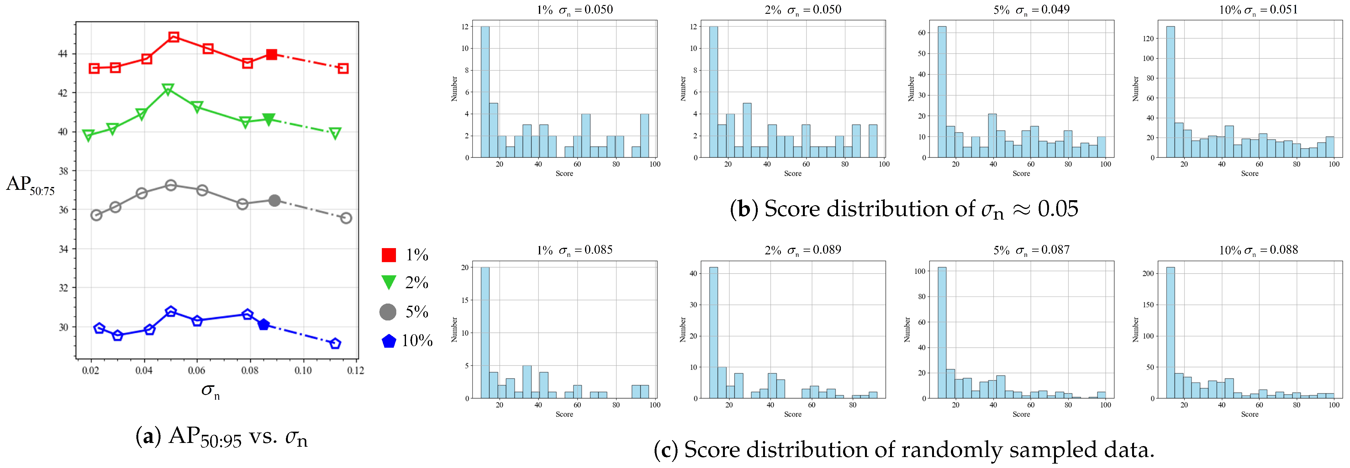
3.1.3. Choice of Appropriate Data

Appropriate training data were selected by interval sampling according to a certain C S distribution. According to the C S distribution of all data, the gray-scale values were manually divided into several intervals, and a certain amount of data was randomly sampled in different intervals to obtain labeled training data with different C S distributions.
The scores of the selected data were divided into 20 intervals, and the data number n i of each interval was calculated. Their standard deviation can be used as a reference index to measure whether the data distribution is uniform: the smaller the standard deviation, the more uniform the distribution is. However, the different data amounts are different even if they are based on the same standard deviation, so the normalized standard deviation of these 20 intervals can be obtained by dividing the standard deviation with the amount of data to obtain the evenness index:
σ n = 1 N l i = 1 20 n i n ¯ 20
where n ¯ = N l / 20 denotes the mean value of n i .

3.2. Orientation-Angle Deviation Weighting Loss

We designed the orientation deviation weighting (ODW) loss as the unsupervised loss to enhance the performance of semi-supervised learning. In supervised learning, the ground truth is used as a reliable reference, and the prediction results will be forced to move closer to it. However, in semi-supervised learning, we cannot simply take the pseudo-labels, generated by the teacher model, as the ground truth, and copying the supervised training will cause the effect of semi-supervised learning to deteriorate in a positive feedback style: the student model learns the wrong information from the unreliable pseudo-labels generated by the teacher model, and the EMA-updated teacher model continuously obtains the wrong “cognition” and generates more unreliable pseudo-labels, eventually leading to the deterioration of the performance of semi-supervised training.
The overall loss is defined as the weighted sum of the supervised and unsupervised losses:
L = L l + λ L u
where L l and L u denote the supervised loss of labeled images and the unsupervised loss of unlabeled images, respectively, and L u = L OWD . λ indicates the importance of the unsupervised loss. Both of them are normalized by the respective number of images in the training data batch:
L l = 1 N l i = 1 N l L cls I l i + L bbox I l i + L ctrness I l i L u = L OWD = 1 N u i = 1 N u L cls I u i + L bbox I u i + L ctrness I u i
where I l i and I u i denote the i-th labeled and unlabeled image, respectively. L cls , L bbox , and L ctrness are the classification loss, bounding box loss, and centerness loss, respectively. N l and N u indicate the number of labeled and unlabeled images, respectively. The bounding box loss, i.e., L1 loss, of the pseudo-label prediction pair is replaced by the Gaussian Wasserstein distance (GWD) loss, while the classification loss and centerness loss still adopt the focal loss and binary cross-entropy (BCE) loss.
Considering that the difference in orientation-angle between pseudo-label prediction pairs can reflect the difficulty of the sample to a certain extent, this deviation can be used as a weight to adaptively adjust the unsupervised loss. All the unsupervised losses were dynamically weighted by the orientation-angle deviation of the pseudo-label prediction pairs as the final unsupervised loss. The unsupervised bounding box losses are shown in Equation (12), and the classification loss and centerness loss have similar forms. The supervised loss is also similar, but without weight w j .
L bbox I u = 1 N p j = 1 N p w j L GWD ( B s j , B t j )
where N p represents the number of pseudo-label prediction pairs for each image, L GWD ( B s j , B t j ) denotes the GWD loss of the j-th pseudo-label prediction pairs, while B s and B t are the bounding boxes of the student model prediction and pseudo-label generated by the teacher model, respectively. The calculation method for the weight w j is shown as follows:
Huber θ s , θ t = ( θ s θ t ) 2 δ ( 2 π δ ) , θ s θ t δ θ s θ t 0.5 δ π 0.5 δ , θ s θ t > δ w j = 1 + α Huber ( θ s j , θ t j )
where θ s and θ t are the oriented angles of the student model’s prediction and pseudo-label. α and δ are hyper-parameters reflecting the importance of the orientation and the smoothness of the Huber loss, which can be empirically set as 50 and 1, respectively.
Sometimes, a small training loss does not mean a better result of detection, due to the inconsistency of the metric and loss function: such as the rotated intersection over union (RIoU) and smooth L1 loss. When using the smooth L1 loss, there are boundary discontinuity and square-like problems whether OpenCV or Long Edge is adopted as the bounding box definition. Therefore, we adopted the Gaussian Wasserstein distance (GWD) loss between the pseudo-labels and the student’s predicting results, instead of the smooth L1 loss.
As shown in Figure 7, the GWD converts an oriented bounding box B ( x , y , w , h , θ ) into a 2D Gaussian distribution N ( μ , Σ ) . The detailed calculation process is expressed as follows:
Σ 1 / 2 = R Λ R T = cos θ sin θ sin θ cos θ w 2 0 0 h 2 cos θ sin θ sin θ cos θ = w 2 cos 2 θ + h 2 sin 2 θ w h 2 cos θ sin θ w h 2 cos θ sin θ w 2 sin 2 θ + h 2 cos 2 θ μ = ( x , y ) T
where R and Λ represent the rotation matrix and the diagonal matrix of the eigenvalues, respectively.
The GWD between two probability distribution measures X s N s μ s , Σ s and X t N t μ t , Σ t can be expressed as:
D w N s , N t 2 = μ s μ t 2 2 + Tr Σ s + Σ t 2 Σ s 1 / 2 Σ t Σ s 1 / 2 1 / 2
The final form of the GWD loss is:
L GWD ( B s , B t ) = 1 1 τ + f D w N s , N t 2
where f ( · ) represents a nonlinear function to make the loss smoother and more expressive. In this paper, we set D w 2 as the nonlinear function and τ = 2 .

4. Experiments and Analysis

4.1. Datasets’ Description

The Rotated Ship Detection Dataset in SAR images (RSDD-SAR) [44] mainly used in this paper was prepared for oriented ship detection, containing a training set of 5000 images and a test set of 2000 images, which were taken from 84 Gaofen-3 data, 41 TerraSAR-X data, and two original large images, totaling 127 scenes. The images in the dataset contain different latitudes and longitudes, acquisition times, imaging modes, resolutions, polarimetric modes, incidence angles, and imaging widths. The oriented bounding box definition method of RSDD-SAR is the Long Edge definition, as shown in Figure 8, and the unit of the angles is radians. Because RSDD-SAR has more diverse sources, we used it as the primary dataset for semi-supervised learning.
Three additional datasets were also used in this study: SAR Ship Detection Dataset (SSDD) [45], High-Resolution SAR Images Dataset (HRSID) [46], and Large-Scale SAR Ship Detection Dataset (LS-SSDD) [47]. The SSDD is the first open dataset that has been widely used to research the state-of-the-art technology of DL-based SAR ship detection. In the SSDD, there are typical hard to detect samples that need special consideration in practical SAR ship-detection applications, such as small ships with inconspicuous features, densely parallel ships berthing at ports with overlapping hulls, and ships with large-scale differences. The HRSID is the first SAR ship dataset that supports instance segmentation. It has richer data sources and scenes compared to the SSDD, but it uses only high-resolution SAR images. The LS-SSDD contains 15 large-scale SAR images, accurately labeled with the aid of the automatic identification system (AIS) and Google Earth. When all the training images in the RSDD-SAR dataset were taken as labeled data, we used all the images in the other three datasets as unlabeled data for extended experiments, and the summary of these four datasets is shown in Table 2.
The following two settings were mainly studied:
  • RSDD-SAR: There were 1%, 2%, 5%, and 10% of the 5000 training data selected as labeled data by random sampling and RDS sampling, respectively, and the remaining training data were selected as unlabeled data for semi-supervised training.
  • Mixture datasets: All 5000 training data of RSDD-SAR were taken as labeled data, and a total of 15764 images from the SSDD, HRSID, and LS-SSDD were taken as the unlabeled dataset for extended experiments.

4.2. Implementation Details

The following are the implementation details of the experiments in this paper. The experiments employed training and testing under the Ubuntu 22.04 operating system, using two Nvidia RTX 3090 graphics processing units (GPU), and the CPU was an AMD EPYC 75F3 32-Core Processor. The versions of CUDA, Pytorch, and Python for the experimental environment were 12.2, 1.13.0, and 3.9. We carried out our algorithm implementation and hyper-parameter settings on the unified rotated object detection toolbox (MMRotate [48]).
Without loss of generality, we took FCOS [49] as the representative anchor-free detector and adopted the pretrained ResNet-50 [50] as the backbone for all our experiments. The hyper-parameters of the experiment were set as follows: The optimizer used was stochastic gradient descent (SGD), with a momentum of 0.9 and a weight decay of 1 ×   10 4 . The learning rate was initialized to 2.5 ×   10 3 and linearly increased from 0 to 1 ×   10 3 in the first 500 steps through preheating. All models were trained for 36,000 iterations. At the 16,000th iteration and 22,000th iteration, the learning rate decreased to one-tenth of the original. For both labeled or unlabeled data, the training batch size was set to 4. All images were uniformly scaled to 512 × 512, and the ratio between the labeled and unlabeled data was 1:2.
The EMA began with the 100th iteration, with the EMA rate and interval set to 0.9996 and 1, respectively. The first 6400 iterations of the training were the “burn-in” stage, and after the burn-in stage, the same data augmentations as in [5] were applied. In the second 6400 iterations, the weight of the unsupervised learning losses λ increased linearly from 0 to 1 and remained 1 after that.

4.3. Evaluation Metrics

The average precision was used to evaluate the detection performance. The precision and recall measure the proportion of true positive detections in the total prediction results and total targets, respectively, and can be calculated as:
P = N tp N pred , R = N tp N targets
where N tp , N pred , and N targets denote the number of objects correctly detected, the total number of prediction results, and real number of targets, respectively.
After the threshold of the RIoU was given, R was taken as the horizontal coordinate, and P was taken as the vertical coordinate. The detection results were sorted from high to low by the confidence metric, and the precision–recall curve was obtained by adjusting the confidence threshold. The average detection precision AP was obtained by integrating the precision–recall curve. The higher the average detection precision AP was, the better the model’s performance was. Its calculation formula is shown as follows:
AP = 0 1 P ( R ) d R
When the RIoU threshold was set to 0.5 and 0.75, the AP obtained was correspondingly denoted as AP 50 and AP 75 , the latter being a high-precision metric. In addition, metric AP 50 : 95 is calculated as follows:
AP 50 : 95 = i = 0.5 0.95 A P i

4.4. Main Results and Analysis

4.4.1. Results of FCE

As shown in Figure 9, the scenes in the picture from left to right are gradually more complex: the leftmost is basically a calm sea, with fewer strong scattering points, except for ships and a more concentrated gray-scale value distribution; the right picture has a large land or strong sea clutter, and the gray-scale value distribution is more dispersed, while the overall intensity is higher. To achieve better visualization, as shown in the second row in Figure 9, the images were locally enlarged to reveal more details of the ships. These phenomena reflect that, as the images progress from left to right, the mean and variance of the gray-scale values generally increase. This is manifested in the histogram as the peak position and peak width rise accordingly, as shown in the forth in row Figure 9. From the results of the morphological processing, as shown in the third row of Figure 9, we can observe that the spatial distribution of the pixels becomes increasingly complex: the connected regions obtained after processing increase in number, size, and density. Table 3 shows the values of each evaluation index and corresponding to the images shown in Figure 9, and it gives a simple description of the types of scenes in the pictures. Each evaluation indicator shows a general upward trend from left to right, reflecting the complexity of the scene to a certain extent. The comprehensive score C S in the end line is basically consistent with the subjective feelings of scene complexity in the corresponding images, which proves the effectiveness of the scoring mechanism based on FCE.
It should be added that the gray-scale histogram only illustrates the gray-scale value distribution of the JPG image itself, not the amplitude distribution obtained after SAR imaging. Because the producer will truncate parts with a higher amplitude during the dataset-generation process, many gray-scale histograms will show a peak value at 255, which will cause the histogram to not accurately reflect the amplitude distribution of the SAR.
Figure 10 shows the histograms of seven evaluation indicator values and the final comprehensive scores of 5000 images in the RSDD-SAR training set. It can be seen that most of the comprehensive scores of the data in RSDD-SAR are concentrated in a lower interval, consistent with humans’ subjective feeling about the data. This illustrates the effectiveness of the proposed evaluation method. Now, appropriate membership parameters can be selected according to the distribution of the seven evaluation indicators as follows:
a μ , b μ , c μ , d μ , e μ , f μ = { 10 , 20 , 30 , 40 , 50 , 60 } a σ 2 , b σ 2 , c σ 2 , d σ 2 , e σ 2 , f σ 2 = { 400 , 800 , 1200 , 1600 , 2000 , 2400 } a S F , b S F , c S F , d S F , e S F , f S F = { 2 , 4 , 6 , 8 , 10 , 12 } a N P , b N P , c N P , d N P , e N P , f N P = { 1 , 1.5 , 2 , 2.5 , 3 , 3.5 } a P H , b P H , c P H , d P H , e P H , f P H = { 11 , 22 , 33 , 44 , 55 , 66 } a w , b w , c w , d w , e w , f w = { 15 , 30 , 45 , 60 , 75 , 90 } a P W , b P W , c P W , d P W , e P W , f P W = { 15 , 30 , 45 , 60 , 75 , 90 }

4.4.2. Relationship between Detection Performance and Data Distribution

The training results with variable data distributions and proportions of labeled data are depicted in Figure 11a, and it is worth noting that the σ n of the data, obtained by random sampling, was around 0.88. It is evident that the performance improved with higher proportions of labeled data, particularly when σ n was around 0.05, showing optimal performance. Although there is a significant reduction in the simple scene data in Figure 11b, compared to the random sampling in Figure 11c, a considerable amount of simple scene data were still retained in the selected data. It is crucial to ensure the model learns effective information and efficiently avoids overfitting on incorrect details in complex scenes.
Similar to human learning, rich basic knowledge facilitates a better understanding of complex concepts. Likewise, in model training, an adequate amount of basic data helps to learn complex data. Thus, when the data volume reached a certain threshold, augmenting complex scene data yielded better performance improvements compared to an equivalent volume of simple scene data.

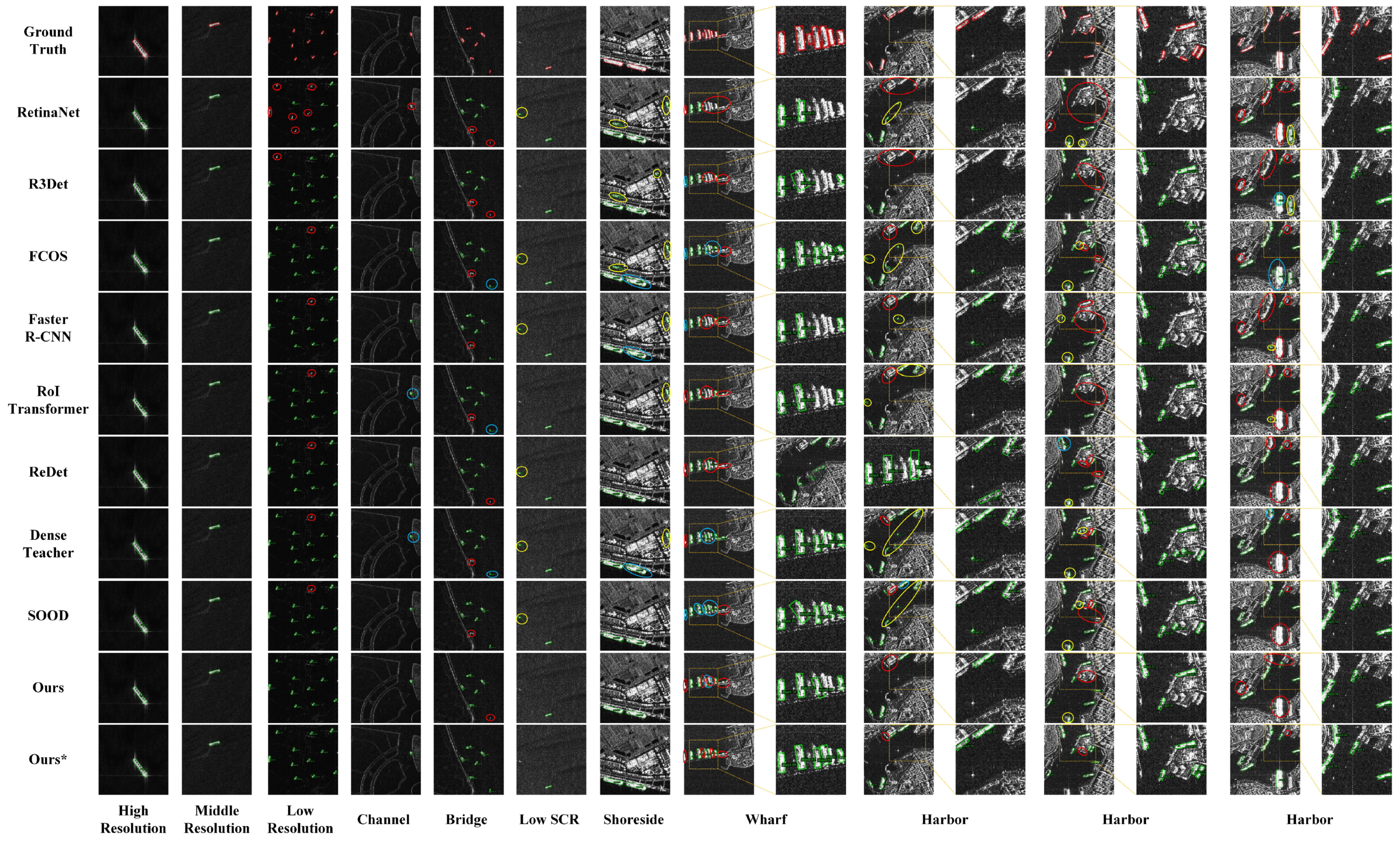
4.4.3. Comparison with Representative Methods

In this section, we compare the proposed methods with the Dense Teacher and SOOD semi-supervised methods on the RSDD-SAR dataset. All semi-supervised learning methods used the same data augmentation.

Partially Labeled Data

We firstly performed the evaluation using partially labeled data, and the results are shown in Table 4. In addition, six supervised methods are compared here: RetinaNet [51], R3Det [52], FCOS, i.e., three single-stage methods and Faster R-CNN [53], RoI Transformer [54], and ReDet [55], i.e., three classical two-stage methods. The proposed method includes whether the RDS is used or not. Overall, under the same amount of data, the performance of the semi-supervised learning methods surpassed that of the supervised learning methods, and the two-stage object detection algorithms outperformed the single-stage algorithms. However, when the data volume was small, the two-stage methods tended to overfit, due to their larger number of parameters, resulting in poorer performance compared to the single-stage FCOS. It is obvious that, with the increase in the number of labeled data, the detection performance of all methods improved. At the same time, it can also be seen that, when the proportion of labeled data was 1%, 2%, 5%, and 10% without the RDS, our method increased by 2.95%, 4.00%, 3.20%, and 1.18%, respectively, compared with SOOD. After using the RDS, they further increased by 0.53%, 0.77%, 1.55%, and 0.89% percentage points, respectively. The qualitative comparison results with 10% labeled data are shown in Figure 12.
As shown in Figure 12, the scenes in the five images on the left are relatively simple, and the detection performance of the other methods, except for RetinaNet, is relatively good. In low-SCR scenarios, most algorithms mistakenly detected interference on the left side of the image as ships, resulting in false alarms. The scenes in the five images on the right are more complex. The proposed method achieved the best detection performance, as indicated by the size and number of circles in the original images. The locally enlarged images also revealed more detailed detection results. Although the proposed method still had some missing detections, it is noteworthy that these results were obtained using only 10% training images.
Combined with the comprehensive score distribution of the dataset in Figure 10h and the qualitative comparison results in Figure 12, on the one hand, most of the data in the dataset were simple data with low scores, and there were relatively few complex scenes. On the other hand, training with or without the RDS selection data in simple scenes had similar performance. However, after using the RDS in challenging scenes, the false alarm rate, missed detection rate, and poor bounding box regression were greatly reduced. The function of the RDS is mainly to improve the detection performance of complex scenarios. Therefore, if there is a higher proportion of complex scene images in the test data, the final AP 50 : 95 will be higher.

Fully Labeled Data

When using all labeled data in RSDD-SAR, all 15,764 images in the SSDD+, HRSID, and LS-SSDD datasets were used as unlabeled data. As shown in Table 5, compared with the supervised FCOS method, the AP 50 : 95 , AP 50 , and AP 75 of the proposed method has been increased by 3.6%, 8.5%, and 7.4%, respectively, and also increased by 1.74%, 0.4%, and 0.5% compared with the baseline method, which proves the ability of the proposed model to make full use of a large amount of unlabeled data. This improvement is due to the fact that unlabeled data and pseudo-labels mitigate the over-fitting of the model to the labeled data to some extent and enable the model to learn more robust representations.
In addition, we can see that the difference between the proposed method with 10% labeled data and the supervised method with fully labeled data on AP 50 : 95 was only 2.56%, which fully demonstrates its superiority.

4.4.4. Ablation Experiment

In this part, we validate two proposed improvements for SOOD, and all ablation experiments were performed on 1% RSDD-SAR labeled data. The model degenerated to the Dense Teacher when the RAW, ODW, and GWD were not used, and SOOD when only the RAW was used. It can be seen from Table 6 that our improvements were effective: adopting the GWD loss as the bounding box loss and the ODW can bring performance gains, respectively. Using these two improvements at the same time can further improve performance. As shown in Figure 13, in scenarios with a high SCR, the bounding box regression accuracy of all methods was high. However, in scenarios with a low SCR and high sidelobe effects, the detection performance of the Dense Teacher and SOOD significantly declined, making effective bounding box regression challenging, as shown in the “Dense Teacher” row and “+RAW” row in Figure 13. After using the GWD, the regression accuracy of the shape and size of the bounding boxes improved, as shown in the “+GWD” row in Figure 13. Furthermore, after applying the ODW, the regression accuracy of the bounding box rotation angle was further enhanced, as shown in the “+ODW” row in Figure 13. When the GWD and ODW were used simultaneously, the model can still perform relatively well even in low-SCR scenarios, where the ship edges were severely affected, as shown in the “+GWD+ODW” row in Figure 13. Since all semi-supervised models used the teacher model for prediction, the results presented here are considered as a comparison of pseudo-label quality. It can be seen that the proposed method significantly improved the quality of the pseudo-labels.

5. Conclusions

In this paper, to reduce the labeling burden and improve the ship detection performance, we propose a semi-supervised oriented SAR ship detection framework from both data and model perspectives. We introduced a simple, but effective scoring method based on FCE for SAR ship detection data. We also studied the influence of the scoring distribution of labeled data on the training results of the semi-supervised model. The RDS enhanced the training effectiveness of the model by selecting more reasonably distributed data. The use of the GWD loss and the ODW loss improved the detection performance of the semi-supervised model in complex scenarios. The effectiveness of these proposed methods was validated through experiments. When creating a new SAR ship detection dataset, the RDS proposed in this paper can select appropriately distributed data for labeling. Subsequently, the semi-supervised model can be utilized for training. In the future, methods such as active learning and clustering can be used to further improve the quality of the selected data.

Author Contributions

Conceptualization, Y.Y. and J.Y. (Jian Yang); methodology, Y.Y.; software, Y.Y.; validation, Y.Y. and P.L.; formal analysis, Y.Y. and P.L.; investigation, Y.Y.; resources, J.Y. (Junjun Yin); data curation, Y.Y.; writing—original draft preparation, Y.Y.; writing—review and editing, Y.Y.; visualization, Y.Y.; supervision, P.L. and Y.H.; project administration, J.Y. (Jian Yang) and J.Y. (Junjun Yin); funding acquisition, J.Y. (Jian Yang) and J.Y. (Junjun Yin). All authors have read and agreed to the published version of the manuscript.

Funding

This work was partly supported by the NSFC under Grant No. 62222102 and NSFC Grant No. 62171023.

Data Availability Statement

The original data presented in the study are openly available in [RSDD-SAR] at https://radars.ac.cn/web/data/getData?dataType=SDD-SAR (accessed on 8 June 2022), [SSDD] at https://www.mdpi.com/2072-4292/13/18/3690 (accessed on 15 September 2021), [LS-SSDD-v1.0] at https://www.mdpi.com/2072-4292/12/18/2997 (accessed on 15 September 2020), and [HRSID] at https://ieeexplore.ieee.org/abstract/document/9127939 (accessed on 29 June 2020).

Conflicts of Interest

The authors declare no conflicts of interest.

Abbreviations

The following abbreviations are used in this manuscript:
AISautomatic identification system
BCEbinary cross-entropy
CFARconstant false alarm rate
DLdeep learning
EMAexponential moving average
GCglobal consistency
GPUGraphics Processing Unit
GWDGaussian Wasserstein distance
HBBhorizontal bounding box
OBBoriented bounding box
ODWorientation-angle deviation weighting
RAWrotation-aware adaptive weighting
RDSrefined data selector
RIoUrotated intersection over union
SARsynthetic aperture radar
SCRSignal-to-Clutter Ratio
SGDstochastic gradient descent
SOODsemi-supervised oriented object detection

References

  1. Li, J.; Xu, C.; Su, H.; Gao, L.; Wang, T. Deep Learning for SAR Ship Detection: Past, Present and Future. Remote Sens. 2022, 14, 2712–2752. [Google Scholar] [CrossRef]
  2. Li, J.; Chen, J.; Cheng, P.; Yu, Z.; Yu, L.; Chi, C. A Survey on Deep-Learning-Based Real-Time SAR Ship Detection. IEEE J. Sel. Top. Appl. Earth Observ. Remote Sens. 2023, 16, 3218–3247. [Google Scholar] [CrossRef]
  3. Meng, L.; Chen, Y.; Li, W.; Zhao, R. Fuzzy Comprehensive Evaluation Model for Water Resources Carrying Capacity in Tarim River Basin, Xinjiang, China. Chin. Geogr. Sci. 2009, 19, 89–95. [Google Scholar] [CrossRef]
  4. Yang, X.; Yan, J.; Ming, Q.; Wang, W.; Zhang, X.; Tian, Q. Rethinking Rotated Object Detection with Gaussian Wasserstein Distance Loss. In Proceedings of the 38th International Conference on Machine Learning (ICML2021), Online, 1 July 2021; pp. 11830–11841. [Google Scholar]
  5. Hua, W.; Liang, D.; Li, J.; Liu, X.; Zou, Z.; Ye, X.; Bai, X. SOOD: Towards Semi-Supervised Oriented Object Detection. In Proceedings of the IEEE/CVF Conference on Computer Vision and Pattern Recognition (CVPR2023), Vancouver, BC, Canada, 18–22 June 2023; pp. 15558–15567. [Google Scholar]
  6. Li, T.; Liu, Z.; Xie, R.; Ran, L. An Improved Superpixel-Level CFAR Detection Method for Ship Targets in High-Resolution SAR Images. IEEE J. Sel. Top. Appl. Earth Observ. Remote Sens. 2018, 11, 184–194. [Google Scholar] [CrossRef]
  7. Wang, X.Q.; Li, G.; Zhang, X.P.; He, Y. A Fast CFAR Algorithm Based on Density-Censoring Operation for Ship Detection in SAR Images. IEEE Geosci. Remote Sens. Lett. 2021, 28, 1085–1089. [Google Scholar] [CrossRef]
  8. Zhai, L.; Li, Y.; Su, Y. Inshore Ship Detection via Saliency and Context Information in High-Resolution SAR Images. IEEE Geosci. Remote Sens. Lett. 2016, 13, 1870–1874. [Google Scholar] [CrossRef]
  9. Pappas, O.; Achim, A.; Bull, D. Superpixel-Level CFAR Detectors for Ship Detection in SAR Imagery. IEEE Geosci. Remote Sens. Lett. 2018, 15, 1397–1401. [Google Scholar] [CrossRef]
  10. Li, T.; Liu, Z.; Ran, L.; Xie, R. Target Detection by Exploiting Superpixel-Level Statistical Dissimilarity for SAR Imagery. IEEE Geosci. Remote Sens. Lett. 2018, 15, 562–566. [Google Scholar] [CrossRef]
  11. Wang, X.Q.; Li, G.; Zhang, X.P.; He, Y. Ship detection in SAR images via local contrast of Fisher vectors. IEEE Trans. Geosci. Remote Sens. 2020, 58, 6467–6479. [Google Scholar] [CrossRef]
  12. Gao, G.; Shi, G. CFAR Ship Detection in Nonhomogeneous Sea Clutter Using Polarimetric SAR Data Based on the Notch Filter. IEEE Trans. Geosci. Remote Sens. 2017, 55, 4811–4824. [Google Scholar] [CrossRef]
  13. Liu, T.; Yang, Z.; Yang, J.; Gao, G. CFAR Ship Detection Methods Using Compact Polarimetric SAR in a K-Wishart Distribution. IEEE J. Sel. Top. Appl. Earth Observ. Remote Sens. 2019, 12, 3737–3745. [Google Scholar] [CrossRef]
  14. Liu, T.; Zhang, J.; Gao, G.; Yang, J.; Marino, A. CFAR Ship Detection in Polarimetric Synthetic Aperture Radar Images Based on Whitening Filter. IEEE Trans. Geosci. Remote Sens. 2019, 58, 58–81. [Google Scholar] [CrossRef]
  15. Zhang, T.; Yang, Z.; Gan, H.P.; Xiang, D.L.; Zhu, S.; Yang, J. PolSAR Ship Detection Using the Joint Polarimetric Information. IEEE Trans. Geosci. Remote Sens. 2020, 58, 8225–8241. [Google Scholar] [CrossRef]
  16. Zhang, T.; Ji, J.S.; Li, X.F.; Yu, W.X.; Xiong, H.L. Ship Detection From PolSAR Imagery Using the Complete Polarimetric Covariance Difference Matrix. IEEE Trans. Geosci. Remote Sens. 2019, 57, 2824–2839. [Google Scholar] [CrossRef]
  17. Liao, M.S.; Wang, C.C.; Wang, Y.; Jiang, L.M. Using SAR Images to Detect Ships From Sea Clutter. IEEE Geosci. Remote Sens. Lett. 2008, 5, 194–198. [Google Scholar] [CrossRef]
  18. Xing, X.W.; Ji, K.F.; Zou, H.X.; Sun, J.X.; Zhou, S.L. High resolution SAR imagery ship detection based on EXS-C-CFAR in Alpha-stable clutters. In Proceedings of the IEEE International Geoscience and Remote Sensing Symposium (IGARSS2011), Vancouver, BC, Canada, 24–29 July 2011; pp. 316–319. [Google Scholar]
  19. Cui, Y.; Yang, J.; Yamaguchi, Y. CFAR ship detection in SAR images based on lognormal mixture models. In Proceedings of the 3rd International Asia-Pacific Conference on Synthetic Aperture Radar (APSAR2011), Seoul, Republic of Korea, 26–30 September 2011; pp. 1–3. [Google Scholar]
  20. Ai, J.Q.; Pei, Z.L.; Yao, B.D.; Wang, Z.C.; Xing, M.D. AIS Data Aided Rayleigh CFAR Ship Detection Algorithm of Multiple-Target Environment in SAR Images. IEEE Trans. Aerosp. Electron. Syst. 2022, 58, 1266–1282. [Google Scholar] [CrossRef]
  21. Bezerra, D.X.; Lorenzzetti, J.A.; Paes, R.L. Marine Environmental Impact on CFAR Ship Detection as Measured by Wave Age in SAR Images. Remote Sens. 2023, 15, 3441–3458. [Google Scholar] [CrossRef]
  22. Fu, J.; Sun, X.; Wang, Z.; Fu, K. An Anchor-Free Method Based on Feature Balancing and Refinement Network for Multiscale Ship Detection in SAR Images. IEEE Trans. Geosci. Remote Sens. 2020, 59, 1331–1344. [Google Scholar] [CrossRef]
  23. Hu, Q.; Hu, S.; Liu, S. BANet: A Balance Attention Network for Anchor-Free Ship Detection in SAR Images. IEEE Trans. Geosci. Remote Sens. 2022, 60, 5222212. [Google Scholar] [CrossRef]
  24. Chen, B.; Yu, C.; Zhao, S.; Song, H. An Anchor-Free Method Based on Transformers and Adaptive Features for Arbitrarily Oriented Ship Detection in SAR Images. IEEE J. Sel. Top. Appl. Earth Observ. Remote Sens. 2023, 17, 2012–2028. [Google Scholar] [CrossRef]
  25. Zhou, Y.; Jiang, X.; Xu, G.; Yang, X.; Liu, X.; Li, Z. PVT-SAR: An Arbitrarily Oriented SAR Ship Detector with Pyramid Vision Transformer. IEEE J. Sel. Top. Appl. Earth Observ. Remote Sens. 2022, 16, 291–305. [Google Scholar] [CrossRef]
  26. Zhou, S.C.; Zhang, M.; Xu, L.; Yu, D.H.; Li, J.J.; Fan, F.; Zhang, L.Y.; Liu, Y. Lightweight SAR Ship Detection Network Based on Transformer and Feature Enhancement. IEEE J. Sel. Top. Appl. Earth Observ. Remote Sens. 2024, 17, 4845–4858. [Google Scholar] [CrossRef]
  27. Yang, X.; Zhang, X.; Wang, N.; Gao, X. A Robust One-Stage Detector for Multiscale Ship Detection with Complex Background in Massive SAR Images. IEEE Trans. Geosci. Remote Sens. 2021, 60, 5217712. [Google Scholar] [CrossRef]
  28. Wei, S.; Su, H.; Ming, J.; Wang, C.; Yan, M.; Kumar, D.; Shi, J.; Zhang, X. Precise and Robust Ship Detection for High-Resolution SAR Imagery Based on HR-SDNet. Remote Sens. 2020, 12, 167. [Google Scholar] [CrossRef]
  29. Li, D.; Liang, Q.; Liu, H.; Liu, Q.; Liu, H.; Liao, G. A Novel Multidimensional Domain Deep Learning Network for SAR Ship Detection. IEEE Trans. Geosci. Remote Sens. 2021, 60, 5203213. [Google Scholar] [CrossRef]
  30. Sohn, K.; Zhang, Z.; Li, C.L.; Zhang, H.; Lee, C.Y.; Pfister, T. A Simple Semi-Supervised Learning Framework for Object Detection. arXiv 2020, arXiv:2005.04757. [Google Scholar]
  31. Yang, Q.; Wei, X.; Wang, B.; Hua, X.; Zhang, L. Interactive Self-Training With Mean Teachers for Semi-Supervised Object Detection. In Proceedings of the IEEE/CVF Conference on Computer Vision and Pattern Recognition (CVPR2021), Online, 19–25 June 2021; pp. 5937–5946. [Google Scholar]
  32. Xu, M.; Zhang, Z.; Hu, H.; Wang, J.; Wang, L.; Wei, F.; Bai, X.; Liu, Z. End-to-End Semi-Supervised Object Detection with Soft Teacher. In Proceedings of the IEEE/CVF International Conference on Computer Vision (ICCV2021), Online, 11–17 October 2021; pp. 3060–3069. [Google Scholar]
  33. Liu, Y.C.; Ma, C.Y.; He, Z.; Kuo, C.W.; Chen, K.; Zhang, P.; Wu, B.; Kira, Z.; Vajda, P. Unbiased Teacher for Semi-Supervised Object Detection. arXiv 2021, arXiv:2102.09480. [Google Scholar]
  34. Zhou, H.; Ge, Z.; Liu, S.; Mao, W.; Li, Z.; Yu, H.; Sun, J. Dense Teacher: Dense Pseudo-Labels for Semi-Supervised Object Detection. In Proceedings of the European Conference on Computer Vision (ECCV2022), Tel Aviv, Israel, 23–27 October 2022; pp. 35–50. [Google Scholar]
  35. Xu, B.; Chen, M.; Guan, W.; Hu, L. Efficient Teacher: Semi-Supervised Object Detection for Yolov5. arXiv 2023, arXiv:2302.07577. [Google Scholar]
  36. Zhang, J.; Lin, X.; Zhang, W.; Wang, K.; Tan, X.; Han, J.; Ding, E.; Wang, J.; Li, G. Semi-Detr: Semi-Supervised Object Detection with Detection Transformers. In Proceedings of the IEEE/CVF Conference on Computer Vision and Pattern Recognition (CVPR2023), Vancouver, BC, Canada, 17–24 June 2023; pp. 23809–23818. [Google Scholar]
  37. Liu, C.; Zhang, W.; Lin, X.; Zhang, W.; Tan, X.; Han, J.; Li, X.; Ding, E.; Wang, J. Ambiguity-Resistant Semi-Supervised Learning for Dense Object Detection. In Proceedings of the IEEE/CVF Conference on Computer Vision and Pattern Recognition (CVPR2023), Vancouver, BC, Canada, 18–22 June 2023; pp. 15579–15588. [Google Scholar]
  38. Ren, P.; Xiao, Y.; Chang, X.; Huang, P.-Y.; Li, Z.; Gupta, B.B.; Chen, X.; Wang, X. A Survey of Deep Active Learning 2021. arXiv 2020, arXiv:2009.00236. [Google Scholar]
  39. Xie, Y.C.; Lu, H.; Yan, J.C.; Yang, X.K.; Tomizuka, M.; Zhan, W. Active Finetuning: Exploiting Annotation Budget in the Pretraining-Finetuning Paradigm. In Proceedings of the IEEE/CVF Conference on Computer Vision and Pattern Recognition (CVPR2023), Vancouver, BC, Canada, 18–22 June 2023; pp. 23715–23724. [Google Scholar]
  40. Bengar, J.Z.; Weijer, J.; Twardowski, B.; Raducanu, B. Reducing Label Effort: Self-Supervised Meets Active Learning. In Proceedings of the IEEE/CVF International Conference on Computer Vision (ICCV2021), Online, 11–17 October 2021; pp. 1631–1639. [Google Scholar]
  41. Babaee, M.; Tsoukalas, S.; Rigoll, G.; Datcu, M. Visualization-Based Active Learning for the Annotation of SAR Images. IEEE J. Sel. Top. Appl. Earth Observ. Remote Sens. 2015, 8, 4687–4698. [Google Scholar] [CrossRef]
  42. Bi, H.X.; Xu, F.; Wei, Z.Q.; Xue, Y.; Xu, Z.B. An Active Deep Learning Approach for Minimally Supervised PolSAR Image Classification. IEEE Trans. Geosci. Remote Sens. 2019, 57, 9378–9395. [Google Scholar] [CrossRef]
  43. Zhao, S.Y.; Luo, Y.; Zhang, T.; Guo, W.W.; Zhang, Z.H. Active Learning SAR Image Classification Method Crossing Different Imaging Platforms. IEEE Geosci. Remote Sens. Lett. 2022, 19, 4514105. [Google Scholar] [CrossRef]
  44. Xu, C.A.; Su, H.; Li, W.J.; Liu, Y.; Yao, L.B.; Gao, L.; Yan, W.J.; Wang, T.Y. RSDD-SAR: Rotated Ship Detection Dataset in SAR Images. J. Radars 2022, 11, 581–599. [Google Scholar]
  45. Zhang, T.; Zhang, X.; Li, J.; Xu, X.; Wang, B.; Zhan, X.; Xu, Y.; Ke, X.; Zeng, T.; Su, H. SAR Ship Detection Dataset (SSDD): Official Release and Comprehensive Data Analysis. Remote Sens. 2021, 13, 3690–3730. [Google Scholar] [CrossRef]
  46. Wei, S.; Zeng, X.; Qu, Q.; Wang, M.; Su, H.; Shi, J. HRSID: A High-Resolution SAR Images Dataset for Ship Detection and Instance Segmentation. IEEE Access 2020, 8, 120234–120254. [Google Scholar] [CrossRef]
  47. Zhang, T.; Zhang, X.; Ke, X.; Zhan, X.; Shi, J.; Wei, S.; Pan, D.; Li, J.; Su, H.; Zhou, Y. LS-SSDD-v1. 0: A Deep Learning Dataset Dedicated to Small Ship Detection from Large-Scale Sentinel-1 SAR Images. Remote Sens. 2020, 12, 2997–3033. [Google Scholar] [CrossRef]
  48. Zhou, Y.; Yang, X.; Zhang, G.; Wang, J.; Liu, Y.; Hou, L.; Jiang, X.; Liu, X.; Yan, J.; Lyu, C. MMrotate: A Rotated Object Detection Benchmark Using Pytorch. In Proceedings of the 30th ACM International Conference on Multimedia (ACMMM 2022), Lisbon, Portugal, 10 October 2022; pp. 7331–7334. [Google Scholar]
  49. Tian, Z.; Shen, C.; Chen, H.; He, T. Fcos: Fully Convolutional One-Stage Object Detection. In Proceedings of the IEEE/CVF International Conference on Computer Vision (ICCV2019), Seoul, Republic of Korea, 27 October–2 November 2019; pp. 9627–9636. [Google Scholar]
  50. He, K.; Zhang, X.; Ren, S.; Sun, J. Deep Residual Learning for Image Recognition. In Proceedings of the IEEE/CVF Conference on Computer Vision and Pattern Recognition (CVPR2016), Las Vegas, USA, 27–30 June 2016; pp. 770–778. [Google Scholar]
  51. Lin, T.; Goyal, P.; Girshick, R.; He, K.; Dollar, P. Focal Loss for Dense Object Detection. In Proceedings of the IEEE/CVF International Conference on Computer Vision (ICCV2017), Venice, Italy, 22–29 October 2017; pp. 2980–2988. [Google Scholar]
  52. Yang, X.; Yan, J.; Feng, Z.; He, T. R3Det: Refined Single-Stage Detector with Feature Refinement for Rotating Object. In Proceedings of the AAAI Conference on Artificial Intelligence (AAAI2021), Online, 2–9 February 2021; pp. 3163–3171. [Google Scholar]
  53. Ren, S.; He, K.; Girshick, R.; Sun, J. Faster R-CNN: Towards Real-Time Object Detection with Region Proposal Networks. IEEE Trans. Pattern Anal. Mach. Intell. 2016, 39, 1137–1149. [Google Scholar] [CrossRef]
  54. Ding, J.; Xue, N.; Long, Y.; Xia, G.; Lu, Q. Learning RoI Transformer for Oriented Object Detection in Aerial Images. In Proceedings of the IEEE/CVF Conference on Computer Vision and Pattern Recognition (CVPR2019), Long Beach, CA, USA, 16–20 June 2019; pp. 2849–2858. [Google Scholar]
  55. Han, J.; Ding, J.; Xue, N.; Xia, G. ReDet: A Rotation-Equivariant Detector for Aerial Object Detection. In Proceedings of the IEEE/CVF Conference on Computer Vision and Pattern Recognition (CVPR2021), Online, 19–25 June 2021; pp. 2786–2795. [Google Scholar]
Figure 2. The pipeline of our proposed framework for semi-supervised oriented SAR ship detection. Each input batch contains both labeled and unlabeled data, with labeled data selected offline via the refined data selector (RDS). In the unsupervised training part, the teacher model uses weakly augmented data, while the student model uses strongly augmented data, where only the student model is trained and the teacher model is updated through the exponential moving average (EMA). The unsupervised loss is calculated by combining the prediction maps of the teacher model and the student model, where the bounding box loss is the Gaussian Wasserstein distance (GWD) loss, which is then weighted by the orientation-angle deviation. The supervised training loss is calculated based on the difference between the ground truth and the student model’s predictions on the labeled data. The overall loss is obtained by weighting and summing the supervised training loss and the unsupervised training loss.
Remotesensing 16 02551 g002
Figure 3. Overall structure of this paper.
Remotesensing 16 02551 g003
Figure 4. Schematic diagram of the RDS: firstly, calculate the evaluation indicators of SAR images; then, FCE is used to score the data; finally, select the appropriate data from all the data according to the score. The green histogram represents the score distribution of all data, while the blue histogram represents the score distribution of the selected data.
Remotesensing 16 02551 g004
Figure 5. Two different scenes are compared: The images in the left column are demo images; the middle column contains the histograms of their gray-scale value distribution with the green line as smoothed values; the right column shows the results after morphological processing.
Remotesensing 16 02551 g005
Figure 6. Membership function.
Remotesensing 16 02551 g006
Figure 7. Model of the oriented bounding box as a 2D Gaussian distribution. The right image shows the two-dimensional Gaussian distribution after modeling. The closer to red, the nearer to the center of the ship target.
Remotesensing 16 02551 g007
Figure 8. Schematic diagram of the Long Edge definition method used in RSDD-SAR.
Remotesensing 16 02551 g008
Figure 9. There are eight representative sample images, partially enlarged details, morphological results, and their gray-scale histograms.
Remotesensing 16 02551 g009
Figure 10. The seven blue histograms are the indicator histograms used for FCE, and the green histogram is the final comprehensive score histogram.
Remotesensing 16 02551 g010
Figure 11. The influence of labeled data distribution on training performance. In Figure (a), the solid data points are obtained by random sampling, while the hollow data points are obtained by RDS sampling.
Remotesensing 16 02551 g011
Figure 12. The visual comparison results of the algorithms mentioned in Table 4, where the red circle indicates missing detection, the yellow circle indicates false alarm, and the blue circle indicates poor regression results of the bounding box. The fewer and smaller the circles, the better the algorithm’s performance. The images of the wharf and harbor are locally enlarged to achieve better visualization. * indicates that the RDS is adopted.
Remotesensing 16 02551 g012
Figure 13. The visualization results of the ablation experiments are presented. The first row shows the ground truth. In the scenes of the first two columns, the SCR is high, and the edges of the ships are clear. In the scenes of the last five columns, the SCR is low, or the edges of the ships are affected by high sidelobes.
Remotesensing 16 02551 g013
Table 1. Descriptions and functions of different components.
ComponentDescriptionFunction
RDSSelect appropriate indicators to evaluate SAR images; use FCE for comprehensive assessment; filter data based on the final scores.Obtain scores for SAR images, and acquire a higher quality SAR dataset.
Spatial CharacteristicsObtained from the number, area, and spacing of connected regions after binarization, dilation, and other morphological operations.Describing the spatial distribution of high-intensity pixels in SAR images and used as evaluation indicators for FCE.
Statistical CharacteristicsIncluding the mean and variance of SAR image gray-scale values, as well as some features of the histogram.Describing the statistical distribution of SAR image pixels and used as evaluation indicators for FCE.
FCEMembership functions are derived from the distribution of evaluation indicators, and single factor evaluation is performed for different indicators. The final score is calculated using the weighted average fuzzy product.Obtain comprehensive scores for SAR images for data-selection purposes.
Select Appropriate DataAfter obtaining the final scores, data selection is performed through interval sampling.As the name implies.
Semi-Supervised Oriented SAR Ship DetectionA teacher–student model that combines supervised and unsupervised learning, using ODW loss as the unsupervised learning
loss function.
Make full use of existing labeled data, and leverage a large amount of unlabeled data to improve generalization ability.
Teacher-Student ModelDuring the unsupervised learning phase, only the student model is trained, and the teacher model is updated using the EMA at the end of
each iteration.
It allows for end-to-end semi-supervised learning.
ODW LossThe deviation between the student model’s predictions and the teacher model’s generated pseudo-labels is used as the weights to dynamically weight the unsupervised training loss.This improves the accuracy of the model’s bounding box angle regression.
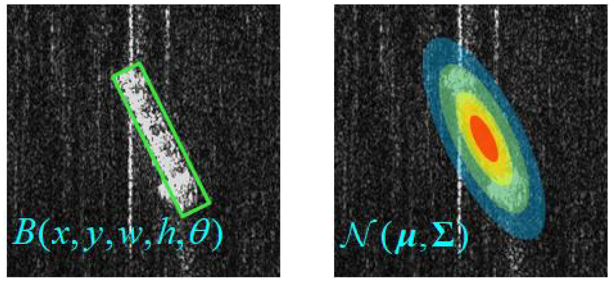
GWD LossThe OBB is modeled as a two-dimensional Gaussian distribution, and the Wasserstein distance between the student model’s predictions and the pseudo-labels, as well as the ground truth, is calculated as the bounding box regression loss function.As part of the ODW loss, this approach enhances the accuracy of the model’s bounding box predictions, especially in low-SCR and high sidelobe effect scenarios.
Table 2. Summary of the SAR ship datasets in this article.
DatasetResolution (m)Image SizeNumber of ImagesNumber of ShipsAnnotations
RSDD-SAR2–20512700010,263OBB
SSDD+1–15214–66811602540OBB
HRSID0.5, 1, 3800560416,951OBB
LS-SSDD 15 × 2080090006016HBB
1 Image slices obtained from 15 large-scene SAR images.
Table 3. Descriptions, different indicators, and the final comprehensive score ( C S ) of the eight images shown in Figure 9.
Image 1Image 2Image 3Image 4Image 5Image 6Image 7Image 8
DescriptionOffshoreBridgeInshoreIslandLow SCRShoresideHarborHarbor
μ 8.622.438.327.651.371.882.279.1
σ 2 156.9512.21230.61000.9822.66256.55778.76900.2
S F 2.33.48.15.713.55.76.910.8
N P 12341334
P H 8.08.016.08.040.0248.056.0248.0
w16.040.048.0112.072.0112.0248.0144.0
P W 8.08.016.088.040.032.0240.0112.0
CS 11.327.649.754.665.077.584.191.3
Table 4. Experimental results of AP 50 : 95 on RSDD-SAR under the partially labeled data setting. Experiments were conducted on 1%, 2%, 5%, and 10% labeled data settings. * indicates that the RDS is adopted and σ n 0.05 .
SettingMethod1%2%5%10%
SupervisedRetinaNet18.95 ± 0.5223.23 ± 0.2330.45 ± 0.1434.77 ± 0.16
R3Det21.73 ± 0.3326.92 ± 0.1733.62 ± 0.2137.23 ± 0.23
FCOS23.44 ± 0.1828.07 ± 0.2434.92 ± 0.2538.40 ± 0.21
Faster R-CNN23.15 ± 0.4528.88 ± 0.3435.30 ± 0.2439.01 ± 0.18
RoI Transformer22.88 ± 0.3227.92 ± 0.1934.41 ± 0.1839.08 ± 0.17
ReDet23.03 ± 0.2428.54 ± 0.2235.32 ± 0.1739.12 ± 0.09
Semi-supervisedDense Teacher26.56 ± 0.1631.19 ± 0.3636.39 ± 0.1140.42 ± 0.12
SOOD27.14 ± 0.2532.48 ± 0.2037.42 ± 0.1542.79 ± 0.14
Ours30.09 ± 0.1436.48 ± 0.2440.62 ± 0.3143.97 ± 0.18
Ours *30.62 ± 0.4037.25 ± 0.2242.17 ± 0.1844.86 ± 0.23
Table 5. Experiment results on full RSDD-SAR with additional datasets.
Method AP 50 : 95 AP 50 AP 75
Supervised47.3785.7048.40
Dense Teacher48.73 (+1.36)88.40 (+2.70)50.90 (+2.50)
SOOD49.23 (+1.86)88.80 (+3.10)51.30 (+2.90)
Ours50.97 (+3.60)89.20 (+3.50)52.80 (+4.40)
Table 6. Impact of the GWD and ODW. indicates that the corresponding component is used.
RAW 1ODWGWD1%
AP 50 : 95 AP 50 AP 75
---26.5658.0016.40
--27.14 (+0.58)63.00 (+5.00)16.70 (+0.30)
--28.65 (+2.09)64.60 (+6.60)17.60 (+1.20)
--28.95 (+2.39)66.20 (+8.20)18.70 (+2.30)
-30.09 (+3.53)68.00 (+10.00)19.60 (+3.20)
1 SOOD adopted the RAW loss and GC loss in the Dense Teacher. However, since there is only one category in ship detection, the GC loss was not used, so it is not listed here.
Disclaimer/Publisher’s Note: The statements, opinions and data contained in all publications are solely those of the individual author(s) and contributor(s) and not of MDPI and/or the editor(s). MDPI and/or the editor(s) disclaim responsibility for any injury to people or property resulting from any ideas, methods, instructions or products referred to in the content.

