Enhancing the Performance of Machine Learning and Deep Learning-Based Flood Susceptibility Models by Integrating Grey Wolf Optimizer (GWO) Algorithm

Abstract

Flooding is a recurrent hazard occurring worldwide, resulting in severe losses. The preparation of a flood susceptibility map is a non-structural approach to flood management before its occurrence. With recent advances in artificial intelligence, achieving a high-accuracy model for flood susceptibility mapping (FSM) is challenging. Therefore, in this study, various artificial intelligence approaches have been utilized to achieve optimal accuracy in flood susceptibility modeling to address this challenge. By incorporating the grey wolf optimizer (GWO) metaheuristic algorithm into various models—including recurrent neural networks (RNNs), support vector regression (SVR), and extreme gradient boosting (XGBoost)—the objective of this modeling is to generate flood susceptibility maps and evaluate the variation in model performance. The tropical Manimala River Basin in India, severely battered by flooding in the past, has been selected as the test site. This modeling utilized 15 conditioning factors such as aspect, enhanced built-up and bareness index (EBBI), slope, elevation, geomorphology, normalized difference water index (NDWI), plan curvature, profile curvature, soil adjusted vegetation index (SAVI), stream density, soil texture, stream power index (SPI), terrain ruggedness index (TRI), land use/land cover (LULC) and topographic wetness index (TWI). Thus, six susceptibility maps are produced by applying the RNN, SVR, XGBoost, RNN-GWO, SVR-GWO, and XGBoost-GWO models. All six models exhibited outstanding (AUC above 0.90) performance, and the performance ranks in the following order: RNN-GWO (AUC: 0.968) > XGBoost-GWO (AUC: 0.961) > SVR-GWO (AUC: 0.960) > RNN (AUC: 0.956) > XGBoost (AUC: 0.953) > SVR (AUC: 0.948). It was discovered that the hybrid GWO optimization algorithm improved the performance of three models. The RNN-GWO-based flood susceptibility map shows that 8.05% of the MRB is very susceptible to floods. The modeling found that the SPI, geomorphology, LULC, stream density, and TWI are the top five influential conditioning factors.

1. Introduction

Flooding, one of the recurrent and deadliest hazards, can result in the loss of lives, enormous losses on property, infrastructure, and livelihood, and impact health and ecosystem services [1,2,3]. Globally, 5582 flood events have been recorded between 1975 and 2022, of which 70% (3913) are riverine flooding [4]. The study conducted by Hirabayashi et al. [5] found that flood exposure is high in Asia, where a 3 °C warming can cause significant flooding. In a study of the GDP loss risk caused by riverine flooding, Zhang et al. [6] learned that the areas with a high-standard risk of GDP loss from riverine flooding are mainly concentrated in Asia, which occurs most often in terms of the number of floods per year for level 1, II, and III floods [7]. Furthermore, they ranked India the third most affected nation among the top 10 countries commonly touched by flooding. Another recent study by Imamura [8] categorized India as a high-flood-risk country. The heavy downpours [9], unplanned development [10], encroachment of flood plains [11], and high population density [12] are the prime drivers of flooding in India. Kerala, a state in India, is very susceptible to floods, with several river basins being regularly affected, especially since 2018 [12,13]. A highly effective susceptibility map is an essential tool for land use planning and risk mitigation actions.

The geographic information system (GIS)-based spatial mapping of flood susceptible zones employed different models, such as conventional statistical methods and knowledge-based methods [14,15]. While traditional statistical methods are model-driven [16,17], the knowledge-based methods solely rely on expert knowledge [18]. Hence, it can result in bias in weight assessments [19]. Machine learning (ML) and deep learning (DL) algorithms have proven efficient when large datasets are available to train the models [20,21]. ML is a data-driven approach that uses data features to generate rules and make decisions or predictions [22], which scientists around the globe are increasingly employing [23]. A variety of ML models were developed that included, but were not limited to, random forest (RF) [24,25], Naive Bayes [24], support vector machine (SVM) [26,27], support vector regression (SVR) [28], k-nearest neighbor (KNN) [29,30], decision trees (DT) [31], CatBoost [32], extreme gradient boosting (XGBoost) [24], gradient boosting [32], and DL models such as convolutional neural networks (CNNs) [33,34], artificial neural networks (ANNs) [23], recurrent neural networks (RNNs) [35,36], and multilayer perceptrons (MLPs) [37] to identify flood-susceptible zones. SVR works well with multidimensional data and provides high predictive accuracy and generalization capacity [38,39]. High and low misestimates are penalized equally, since SVR employs a symmetrical loss function while training [38]. XGBoost can effectively manage missing data and handle extensive and intricate datasets [40]. It can produce more precise outcomes by utilizing decision trees to discover the most significant factors and construct models [41]. XGBoost can effectively handle missing data, and it is also suitable for large and complicated datasets [40]. Decision trees are used in this model to find the most critical factors and build the model. It provides more accurate results. Even though decision trees are utilized, this technique has the advantage of using decision trees to learn about the most essential characteristics; thus, the model is likely to perform better. L1 and L2 regularization are used in XGBoost to prevent overfitting and improve model generalization [42]. The RNN is a conventional neural network structure intended explicitly for sequential input [43]. An RNN can execute the same process with sequential input through recurrent connections. In the event of non-sequential input, an RNN neural network has the same elements as a feedforward neural network, although it will not be able to function. This enables the RNN to store and use data from values that have been analyzed and newly received information [43].

The optimization strategy fine-tunes the hyperparameters to adapt the machine learning models to various tasks, hence enhancing performance [44,45]. According to Yan et al. [46], there are two types of metaheuristic algorithms: population-based and single-solution-based. Due to their low coordination abilities and single-particle scale, only specific complex optimization problems are usually suitable for single-solution-based metaheuristics [47]. Nevertheless, there are advantages to using population-based metaheuristics. These include improved exploration capabilities, more information to guide a set of trial solutions toward a promising area in the search space, and the ability to effectively avoid local optimization caused by the interaction of trial solutions [46]. The grey wolf optimizer (GWO) algorithm is a population-based metaheuristic model that takes its cues from grey wolf hunting and leadership styles [48]. GWO is simple to implement, is easy to understand, has good search precision and speed [49], and requires fewer algorithm parameters for adjustment [46]. Furthermore, GWO has a higher level of optimization performance compared to contemporary algorithms [50].

Two ML regression algorithms, namely SVR and XGBoost, and one DL algorithm, RNN, were used to model the flood susceptibility of a tropical river basin in India. Furthermore, the metaheuristic GWO algorithm was coupled with the ML and DL algorithms to identify if better predictions could be achieved. A comparative analysis was conducted on the performance of all six models, and the study also identified the key components that influence floods. The optimization and refinement of ML and DL models for flood susceptibility modeling in a tropical river basin in India were achieved by applying the metaheuristic algorithm GWO. This is noted because this research represents the pioneer effort to date, since no comprehensive comparison has been conducted on integrating ML and DL algorithms into the GWO algorithm specifically targeted to improve the accuracy of flood susceptibility maps. Such an innovative approach marks this research’s unique contribution to refine further and improve flood susceptibility modeling by harnessing the synergy between GWO and state-of-the-art ML and DL techniques.

2. Materials and Methods

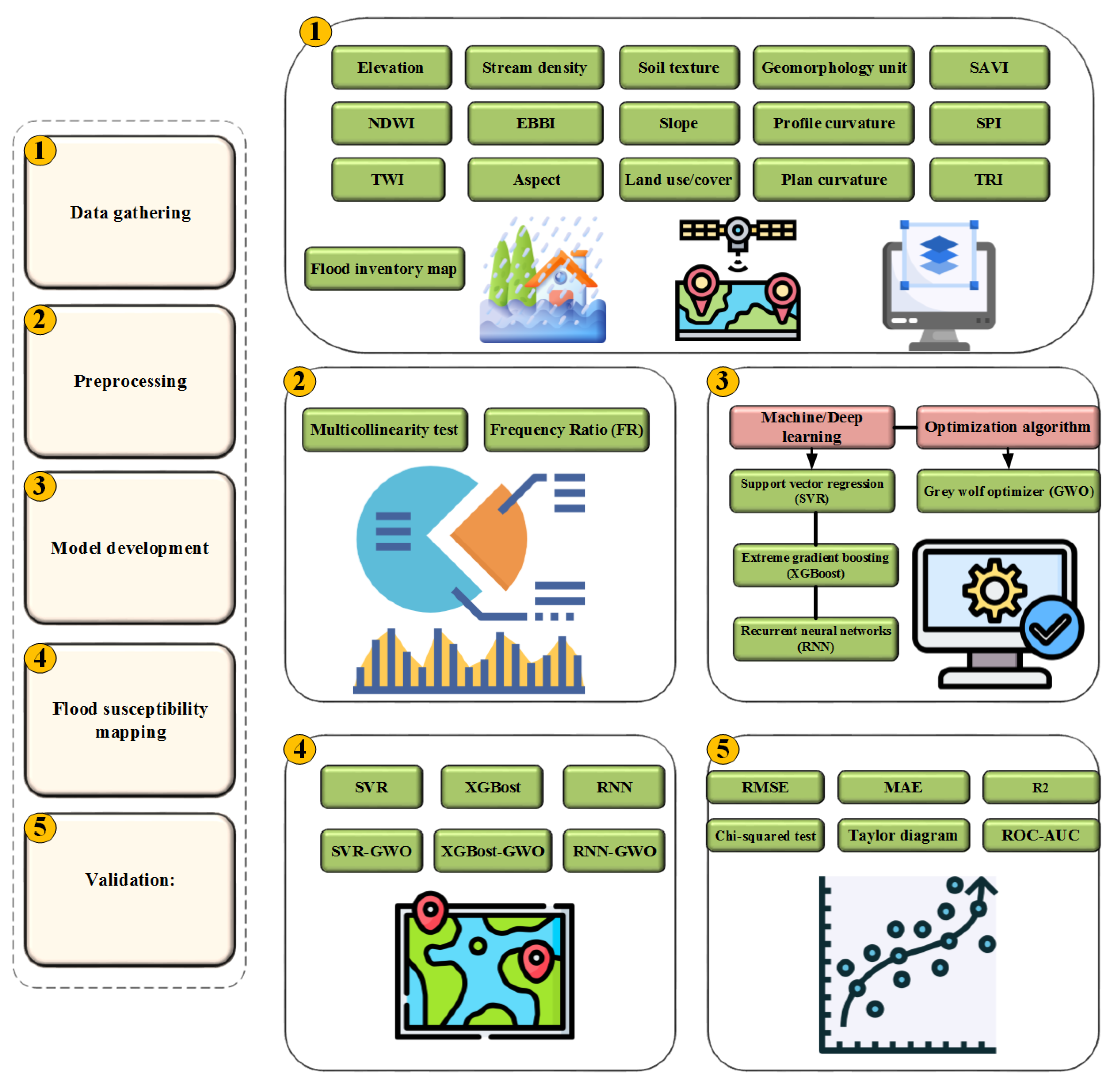
2.1. Methodology

This research is carried out in five significant steps (Figure 1). The first involves collecting data from various sources, including the flood occurrence data and spatial factors affecting floods. In the second step, the collected database was run through preprocessing, which included multicollinearity testing, determining the importance of classes belonging to the factors, and the Frequency Ratio (FR) method of each class of factors. The third step, model development, optimizes SVR, XGBoost, and RNN models using the GWO algorithm. In the next step, flood susceptibility maps were prepared using three standalone models (SVR, XGBoost, and RNN) and three hybrid models (SVR-GWO, XGBoost-GWO, and RNN-GWO) in the ArcGIS 10.8 software. Finally, the developed models and flood susceptibility maps were evaluated in the last step with different statistical indices.

2.2. Study Area

The Manimalayar River, a 92 km long river, flows through the Kerala districts of Idukki, Kottayam, Pathanamthitta, and Alappuzha. The Manimala River Basin (MRB), situated at 1257 m above mean sea level, originates from Kolahalamedu (Muthavara Hills) in the Western Ghats [51]. Rather than emptying directly into the sea, the MRB drains into the Vembanad Lake [51]. The basin is divided into three clearly defined zones: the lowland, the midland, and the highland. Recent data from Senan et al. [12] indicate that the lowland region has been subject to regular floods. The MRB covers 847 km² (Figure 2).

2.3. Flood Inventory Map

Data on flood inundation retrieved from records kept by the National Remote Sensing Centre formed the basis of the flood inventory. The inundation data for 2013, 2018, and 2019 were utilized to create the inventory. Two hundred flood locations were randomly extracted and separated into training and testing datasets following a 70:30 split ratio [52,53]. Figure 3 shows that the training dataset contains 140 sites, and the testing dataset contains 60 flood locations.

2.4. Flood Conditioning Factors

This study considered fifteen factors influencing flood intensification and occurrence. The sources of preparation for each of these influential factors are summarized in

Table 1. Data source.

Data	Source	Conditioning Factors	Spatial Resolution/Scale
ASTER GDEM	https://gdemdl.aster.jspacesystems.or.jp/index_en.html	Slope Elevation Aspect Plan curvature Profile curvature Stream power index (SPI) Terrain ruggedness index (TRI) Topographic wetness index (TWI)	30 m
Landsat-8 OLI image	https://earthexplorer.usgs.gov	Land use/land cover (LULC) types Geomorphic units Enhanced built-up and bareness index (EBBI) Normalized difference water index (NDWI) Soil adjusted vegetation index (SAVI)	30 m
Topographic map	Survey of India (SoI)	Stream density	1:50,000
Soil map	National Bureau of Soil Survey & Land Use Planning (NBSS & LUP)	Soil texture	1:250,000

.

After processing, these factors were prepared with a pixel size of 30 × 30 m (Figure 4). The MRB’s topographic factors were calculated using the ArcGIS 10.8 spatial analyst tools in conjunction with the Advanced Spaceborne Thermal Emission and Reflection Radiometer (ASTER) Global Digital Elevation Model (GDEM). Equations (1)–(3) [54,55,56] were utilized to compute the stream power index (SPI), topographic wetness index (TWI), and terrain ruggedness index (TRI) of the MRB.

$$\mathrm{S}\mathrm{P}\mathrm{I}=\mathsf{\alpha }\times \tan \mathsf{\beta }$$

(1)

$$\mathrm{T}\mathrm{W}\mathrm{I}=\ln \left(\frac{\mathsf{\alpha }}{\tan \mathsf{\beta }}\right)$$

(2)

where α = catchment area, β = slope angle, and tanβ = steepest downslope direction [57].

$$\mathrm{T}\mathrm{R}\mathrm{I}=\sqrt{\mathrm{A}\mathrm{b}\mathrm{s}\left({\mathrm{m}\mathrm{a}\mathrm{x}}^2-{\mathrm{m}\mathrm{i}\mathrm{n}}^2\right)}$$

(3)

The terms “max” and “min” refer to the maximum and lowest values of the cells, as stated by Mojaddadi et al. [56].

The MRB’s land use/cover (LULC) categories were obtained from Landsat-8 images using SAGA 9.3.2 software. The visual interpretation of the Landsat-8 image identified the geomorphic units of this basin. The Landsat 8 OLI image was acquired on 27 January 2023. This is because the dry (non-rainy) season provides clearer landscape views, better vegetation differentiation, and minimal cloud cover, resulting in high-quality data suitable for the precise assessment and classification of LULC types. After analyzing the Landsat-8 image, we utilized Equations (4)–(6) [58,59,60,61] to extract the enhanced built-up and bareness index (EBBI), normalized difference water index (NDWI), and soil-adjusted vegetation index (SAVI), respectively. The stream networks were based on a topographic map provided by the Survey of India. The line density tools of ArcGIS computed the stream density. The soil types of the MRB were obtained using data from the soil map of the National Bureau of Soil Survey and Land Use Planning. The continuous factors such as slope, aspect, altitude, profile curvature, EBBI, NDWI, SAVI, stream density, TWI, TRI, and SPI have been classified utilizing the natural breaks method [53,61], while plan curvature has been classified using the manual method.

$$\mathrm{E}\mathrm{B}\mathrm{B}\mathrm{I}=\frac{\left(\mathrm{S}\mathrm{W}\mathrm{I}\mathrm{R}-\mathrm{N}\mathrm{I}\mathrm{R}\right)}{\sqrt[10]{\left(\mathrm{S}\mathrm{W}\mathrm{I}\mathrm{R}+\mathrm{T}\mathrm{I}\mathrm{R}\right)}}$$

(4)

$$\mathrm{N}\mathrm{D}\mathrm{W}\mathrm{I}=\frac{\left(\mathrm{N}\mathrm{I}\mathrm{R}-\mathrm{S}\mathrm{W}\mathrm{I}\mathrm{R}\right)}{\left(\mathrm{N}\mathrm{I}\mathrm{R}+\mathrm{S}\mathrm{W}\mathrm{I}\mathrm{R}\right)}$$

(5)

$$\mathrm{S}\mathrm{A}\mathrm{V}\mathrm{I}=\left(\frac{\mathrm{N}\mathrm{I}\mathrm{R}-\mathrm{R}\mathrm{e}\mathrm{d}}{\mathrm{N}\mathrm{I}\mathrm{R}+\mathrm{R}\mathrm{e}\mathrm{d}+\mathrm{L}}\right)\times \left(1+\mathrm{L}\right)$$

(6)

L denotes the soil brightness adjustment factor (0.5), and spectral reflectance in the red, near-infrared, short-wavelength, and thermal infrared bands are denoted as NIR, SWIR, and TIR, respectively [58,61].

2.5. Multicollinearity Assessment

Multicollinearity arises when the explanatory variables are too highly correlated with other covariates [62,63]. High multicollinearity can lead to inflated standard errors, making it difficult to determine the individual effect of each predictor variable. The variance inflation factor (VIF) assesses the level of multicollinearity between the explanatory variables [64]. In our case, the VIF was computed for conditioning variables via Equation (7).

$${\mathrm{V}\mathrm{I}\mathrm{F}}_{\mathrm{k}}=\frac{1}{1-{\mathrm{R}}_{\mathrm{k}}^2}$$

(7)

where ${\mathrm{R}}_{\mathrm{k}}^2$ = ${\mathrm{R}}^2$ (R-squared) from the regression of the k^th factor [61,64]. A VIF value greater than 10 indicates a high level of multicollinearity, warranting further action to mitigate it. Therefore, if a factor’s VIF value is higher than 10, that variable should be removed from the modeling process [64].

2.6. Models

2.6.1. Frequency Ratio (FR) Model

To find out how important each category was about the floods, researchers used the frequency ratio (FR) technique. The FR values greater than one show high significance, and those less than one show minor significance [65,66].

$$\mathrm{F}\mathrm{R}=\raisebox{1ex}{$\left(\frac{\mathrm{M}\mathrm{i}}{\mathrm{M}}\right)$}\!\left/ \!\raisebox{-1ex}{$\left(\frac{\mathrm{N}\mathrm{i}}{\mathrm{N}}\right)$}\right.$$

(8)

where Mi = number of flood pixels within a class, M = number of flood pixels, Ni = number of pixels within a class, and Ni = number of pixels [67].

2.6.2. Recurrent Neural Networks (RNNs)

Unlike the traditional neural network, which considers each input to the network as an individual unit, an RNN establishes connections between the units in the hidden layer at different time steps [68,69]. Thus, the information is delivered from one layer to another [69]. Therefore, the RNN algorithm employs internal memory to learn the weights [70]. Let ${\mathrm{x}}_{\mathrm{t}}$ be the input vector, ${\mathrm{h}}_{\mathrm{t}}$ be the hidden vector, and ${\mathrm{y}}_{\mathrm{t}}$ be the output vector; the mathematical representation of these vectors is shown in Equations (9) and (10) [68].

$${\mathrm{h}}_{\mathrm{t}}=\mathsf{\sigma }\left({\mathrm{W}}_{\mathrm{h}}{\mathrm{x}}_{\mathrm{t}}+{\mathrm{U}}_{\mathrm{h}}{\mathrm{h}}_{\mathrm{t}-1}+{\mathrm{b}}_{\mathrm{h}}\right)$$

(9)

$${\mathrm{y}}_{\mathrm{t}}=\mathsf{\sigma }\left({\mathrm{W}}_{\mathrm{y}}{\mathrm{h}}_{\mathrm{t}}+{\mathrm{b}}_{\mathrm{y}}\right)$$

(10)

where W and U = parameter matrices, b = bias vector, and σ (.) = loss function

2.6.3. Support Vector Regression (SVR)

SVR is an ML technique that falls under the category of supervised learning [71]. It can handle nonlinear processes by including a kernel function. This function facilitates the transformation of the initial data into a higher-dimensional space that may be linearly separated [72]. Equation (11) describes the link between input and output variables and will be used to assess the structural risk minimization (SRM) norm [71,73].

$$\mathrm{y}=\mathrm{k}\left(\mathrm{z}\right)=\mathrm{v}\mathrm{\varnothing }\left(\mathrm{z}\right)+\mathrm{c}$$

(11)

where $\mathrm{z}=({\mathrm{z}}_1,{\mathrm{z}}_2,\dots {\mathrm{z}}_{\mathrm{n}})$ represents the input data, and the resultant value will be depicted by ${\mathrm{y}}_{\mathrm{b}}\in {\mathrm{R}}^1$, $\mathrm{v}\in {\mathrm{R}}^1$ = weightage factor, $\mathrm{c}\in {\mathrm{R}}^1$ = constant number, 1 = data size, and $\mathrm{\varnothing }\left(\mathrm{z}\right)$ = irregular function

The following Equations (12) and (13) will be employed to define v and c.

$$\mathrm{M}\mathrm{i}\mathrm{n}\mathrm{i}\mathrm{m}\mathrm{i}\mathrm{z}\mathrm{e}:\left[\frac{1}{2}{‖\mathrm{v}‖}^2+\mathrm{P}{\sum }_{\mathrm{b}=1}^{\mathrm{N}}\left({\mathsf{\zeta }}_{\mathrm{b}}+{\mathsf{\zeta }}_{\mathrm{b}}^{\mathrm{\ast }}\right)\right]$$

(12)

$$\mathrm{S}\mathrm{u}\mathrm{b}\mathrm{j}\mathrm{e}\mathrm{c}\mathrm{t}\mathrm{t}\mathrm{o}:\left\{\begin{array}{c}{\mathrm{y}}_{\mathrm{b}}-\left(\mathrm{v}\mathrm{\varnothing }\left({\mathrm{z}}_{\mathrm{b}}\right)+{\mathrm{c}}_{\mathrm{b}}\right)\le \in +{\mathsf{\zeta }}_{\mathrm{b}}\\ \left(\mathrm{v}\mathrm{\varnothing }\left({\mathrm{z}}_{\mathrm{b}}\right)+{\mathrm{c}}_{\mathrm{b}}\right)-{\mathrm{y}}_{\mathrm{b}}\le \in +{\mathsf{\zeta }}_{\mathrm{b}}^{\mathrm{\ast }}\\ {\mathsf{\zeta }}_{\mathrm{b}},{\mathsf{\zeta }}_{\mathrm{b}}^{\mathrm{\ast }}\ge 0\end{array}\right.$$

(13)

where P = penalty factor, ∈ = optimization performance, and ${\mathsf{\zeta }}_{\mathrm{b}},{\mathsf{\zeta }}_{\mathrm{b}}^{\mathrm{\ast }}$ = loose variables

2.6.4. XGBoost (eXtreme Gradient Boosting)

The XGBoost algorithm utilizes a gradient-boosting methodology that is rooted in decision trees. XGBoost builds decision trees iteratively, and because of higher bias, each of these trees is a weak learner [74]. Sequentially, it produces more trees (weak learners), learns from the previous trees, and corrects until the suitable condition is achieved [74]. XGBoost was implemented using Equation (14) [75].

$$\widehat{{\mathrm{y}}_{\mathrm{i}}}=\mathsf{\varphi }\left({\mathrm{X}}_{\mathrm{i}}\right)=\sum _{\mathrm{k}=1}^{\mathrm{K}}{\mathrm{f}}_{\mathrm{k}}\left({\mathrm{X}}_{\mathrm{i}}\right),{\mathrm{f}}_{\mathrm{k}}\mathsf{ϵ}\mathrm{F}$$

(14)

where F = $\left\{\mathrm{f}\left(\mathrm{x}\right)={\mathrm{w}}_{\mathrm{q}\left(\mathrm{x}\right)}\right\}\left(\mathrm{q}:{\mathrm{R}}^{\mathrm{m}}⇢\mathrm{T},\mathrm{w}\in {\mathrm{R}}^{\mathrm{T}}\right)$ is the function space, and T = number of leaf nodes.

The loss function was computed by applying Equations (15) and (16) [75].

$$\mathrm{L}\left(\mathsf{\varphi }\right)={\sum }_{\mathrm{i}}\mathrm{l}\left({\mathrm{y}}_{\mathrm{i}}{\mathrm{y}}_{\mathrm{i}}\right)+{\sum }_{\mathrm{k}}\mathsf{\Omega }\left({\mathrm{f}}_{\mathrm{k}}\right)$$

(15)

$$\mathsf{\Omega }\left({\mathrm{f}}_{\mathrm{k}}\right)=\mathsf{{\rm Y}}\mathrm{T}+\frac{1}{2}\mathsf{\lambda }{‖\mathrm{w}‖}^2$$

(16)

Equation (15) shows the number of leaves, while Equation (16) shows the size of the result. It was previously mentioned that the gain for each node has been calculated using Equation (17) to check the created branch [75].

$$\mathrm{G}\mathrm{a}\mathrm{i}\mathrm{n}=\frac{1}{2}\left({\mathrm{G}\mathrm{a}\mathrm{i}\mathrm{n}}_{\mathrm{L}}+{\mathrm{G}\mathrm{a}\mathrm{i}\mathrm{n}}_{\mathrm{R}}+{\mathrm{G}\mathrm{a}\mathrm{i}\mathrm{n}}_{\mathrm{O}}\right)-\mathsf{{\rm Y}}$$

(17)

where ${\mathrm{G}\mathrm{a}\mathrm{i}\mathrm{n}}_{\mathrm{O}}$ = gain before splitting, and $\mathsf{{\rm Y}}$ = number of new leaves.

2.6.5. Grey Wolf Optimizer (GWO)

The GWO algorithm emulates grey wolves’ leadership hierarchy and hunting mechanism (Canis lupus) [76]. The hunting behavior simulation will involve four distinct categories of grey wolves: alpha (α), beta (β), delta (δ), and omega (ω) [76]. The three essential phases of hunting behavior will be embedded into the GWO algorithm: spotting the prey, encircling the prey, and attacking the prey. The phases are shown in Equations (18)–(21) [73].

$${\overline{\mathrm{X}}}_{1\left(\mathrm{t}\right)}={\overline{\mathrm{X}}}_{\mathsf{\alpha }\left(\mathrm{t}\right)}-{\overrightarrow{\mathrm{A}}}_1.⋮{\overrightarrow{\mathrm{C}}}_1.{\mathrm{X}}_{\mathsf{\alpha }\left(\mathrm{t}\right)}-{\overrightarrow{\mathrm{X}}}_{\left(\mathrm{t}\right)}$$

(18)

$${\overline{\mathrm{X}}}_{2\left(\mathrm{t}\right)}={\overline{\mathrm{X}}}_{\mathsf{\beta }\left(\mathrm{t}\right)}-{\overrightarrow{\mathrm{A}}}_2.⋮{\overrightarrow{\mathrm{C}}}_2.{\mathrm{X}}_{\mathsf{\beta }\left(\mathrm{t}\right)}-{\overrightarrow{\mathrm{X}}}_{\left(\mathrm{t}\right)}$$

(19)

$${\overline{\mathrm{X}}}_{3\left(\mathrm{t}\right)}={\overline{\mathrm{X}}}_{\mathsf{\delta }\left(\mathrm{t}\right)}-{\overrightarrow{\mathrm{A}}}_3.⋮{\overrightarrow{\mathrm{C}}}_3.{\mathrm{X}}_{\mathsf{\delta }\left(\mathrm{t}\right)}-{\overrightarrow{\mathrm{X}}}_{\left(\mathrm{t}\right)}$$

(20)

$${\overline{\mathrm{X}}}_{(\mathrm{t}+1)}=\frac{1}{3}\left\{{\overrightarrow{\mathrm{X}}}_{1\left(\mathrm{t}\right)}+{\overrightarrow{\mathrm{X}}}_{2\left(\mathrm{t}\right)}+{\overrightarrow{\mathrm{X}}}_{3\left(\mathrm{t}\right)}\right\}$$

(21)

where $\overline{\mathrm{X}}$ is the position vector. Equations (22) and (23) describe the position vector $\overline{X}$, the number of iterations t, and the coefficient vectors $\overrightarrow{\mathrm{A}}$ and $\overrightarrow{\mathrm{C}}$, respectively.

$$\overrightarrow{\mathrm{A}}=2\overrightarrow{\mathrm{a}}.{\overrightarrow{\mathrm{r}}}_1-\overrightarrow{\mathrm{a}}$$

(22)

$$\overrightarrow{\mathrm{C}}=2.{\overrightarrow{\mathrm{r}}}_2$$

(23)

where $\overrightarrow{\mathrm{a}}$ = linearly decreased component, ${\overrightarrow{\mathrm{r}}}_1$ and ${\overrightarrow{\mathrm{r}}}_2$ = random vectors.

2.7. Performance Measures

In this work, we used a selected set of performance metrics to evaluate the efficiency of the proposed models in FSM. These have been designed to secure a clear and complete assessment regarding the performance of the model, especially its accuracy, reliability, and robustness for prediction purposes. The adopted performance metrics are shown below.

2.7.1. Mean Absolute Error (MAE) and Root Mean Squared Error (RMSE)

The mean absolute error (MAE) measures the average deviation between the actual and projected variables. Xu [77] states that the square root of the average deviation between the anticipated and observed variables is the root mean square error (RMSE). The MAE and RMSE measures can take values between zero and infinity with zero being an ideal forecast [78] (Equations (24) and (25)).

$$\mathrm{M}\mathrm{A}\mathrm{E}=\frac{1}{\mathrm{n}}{\sum }_1^{\mathrm{n}}\left|{\mathrm{D}}_{\mathrm{p}\mathrm{r}\mathrm{e}}-{\mathrm{D}}_{\mathrm{a}\mathrm{c}\mathrm{t}}\right|$$

(24)

$$\mathrm{R}\mathrm{M}\mathrm{S}\mathrm{E}=\sqrt{\frac{1}{\mathrm{n}}{\sum }_1^{\mathrm{n}}{\left({\mathrm{D}}_{\mathrm{p}\mathrm{r}\mathrm{e}}-{\mathrm{D}}_{\mathrm{a}\mathrm{c}\mathrm{t}}\right)}^2}$$

(25)

2.7.2. R-Squared (R²)

The value of R² is the fitness of the model, whose value equals the correlation coefficient between the original and their own predicted data squared. Its value ranges from 0 to 1 [78] (Equation (26)).

$${\mathrm{R}}^2=1-\frac{\sum _1^{\mathrm{n}}{\left({\mathrm{D}}_{\mathrm{a}\mathrm{c}\mathrm{t}}-{\mathrm{D}}_{\mathrm{p}\mathrm{r}\mathrm{e}}\right)}^2}{\sum _1^{\mathrm{n}}{\left({\mathrm{D}}_{\mathrm{a}\mathrm{c}\mathrm{t}}-{\overline{\mathrm{D}}}_{\mathrm{a}\mathrm{c}\mathrm{t}}\right)}^2}$$

(26)

where ${\mathrm{D}}_{\mathrm{a}\mathrm{c}\mathrm{t}}$ = actual variable, ${\mathrm{D}}_{\mathrm{p}\mathrm{r}\mathrm{e}}$ = predicted variable, ${\overline{\mathrm{D}}}_{\mathrm{a}\mathrm{c}\mathrm{t}}$ = mean of the actual variable, and n = number of data.

2.7.3. Area under the Receiver Operating Characteristic (ROC) Curve (AUC)

The area under the receiver operating characteristic (ROC) curve is another metric that can be used to measure how well a susceptibility model is doing. According to Melo [79], this metric should be less than or equal to 1 with a range of 0.5 (meaning the model is entirely at random) to 1.0 (indicating a perfect score). According to Hosmer and Lemeshow [80], an area under the curve (AUC) of 0.7–0.8 suggests acceptable performance, an AUC of 0.8–0.9 shows outstanding performance, and an AUC of 0.9 or above indicates exceptional performance.

2.7.4. Chi-Squared Test

The chi-squared test assessed the significance or association between the models. The chi-square value will show the difference between the models [81]. The models are significant when the p-value is less than 0.0001. Equation (27) [81] was used to determine the chi-square values of the models.

$${\mathsf{\chi }}^2={\sum }_{\mathrm{i}=1}^{\mathrm{n}}\frac{{\left({\mathrm{O}}_{\mathrm{i}}-{\mathrm{E}}_{\mathrm{i}}\right)}^2}{{\mathrm{E}}_{\mathrm{i}}}$$

(27)

where ${\mathrm{O}}_{\mathrm{i}}$ = observed frequency in class i, and ${\mathrm{E}}_{\mathrm{i}}$ = expected frequency when no relationship exists between models.

2.7.5. Taylor Diagram

The Taylor diagram is a graph that shows the relationship between the three standard statistical quantifiers: centered root-mean-squared error (CRMSE), standard deviation (σ), and correlation coefficient (R) [82]. The correlation coefficient between variables a and b will be computed employing Equation (28) [83].

$$\mathrm{R}=\frac{\sum _{\mathrm{n}=1}^{\mathrm{N}}\left({\mathrm{a}}_{\mathrm{n}}-\overline{\mathrm{a}}\right)\left({\mathrm{b}}_{\mathrm{n}}-\overline{\mathrm{b}}\right)}{\mathrm{N}{\mathsf{\sigma }}_{\mathrm{a}}{\mathsf{\sigma }}_{\mathrm{b}}}$$

(28)

where N = sample size, ${\mathsf{\sigma }}_{\mathrm{a}}$ and ${\mathsf{\sigma }}_{\mathrm{b}}$ = standard deviations, $\overline{\mathrm{a}}$ and $\overline{\mathrm{b}}$ = time mean, represented as $\overline{\mathrm{a}}$ = $\sum _{\mathrm{n}=1}^{\mathrm{N}}{\mathrm{a}}_{\mathrm{n}}$, $\overline{\mathrm{b}}=\sum _{\mathrm{n}=1}^{\mathrm{N}}{\mathrm{b}}_{\mathrm{n}}$.

The standard deviation will be computed employing Equation (29) [83].

$${\mathsf{\sigma }}_{\mathrm{a}}=\sqrt{\frac{\sum _{\mathrm{n}=1}^{\mathrm{N}}{\left({\mathrm{a}}_{\mathrm{n}}-\overline{\mathrm{a}}\right)}^2}{\mathrm{N}-1}}$$

(29)

CRMSE will be determined by applying Equation (30) [84].

$$\mathrm{C}\mathrm{R}\mathrm{M}\mathrm{S}\mathrm{E}=\sqrt{\frac{1}{\mathrm{N}}}{\sum }_{\mathrm{n}=1}^{\mathrm{N}}{\left[\left({\mathrm{a}}_{\mathrm{n}}-\overline{\mathrm{a}}\right)\left({\mathrm{b}}_{\mathrm{n}}-\overline{\mathrm{b}}\right)\right]}^2$$

(30)

2.7.6. Model Implementation

Python language was used for the implementation and development of flood susceptibility models. The models were executed using Python in the Google Colab programming environment (https://colab.research.google.com/). Initially, 70% of the data was used for the model training. The remaining 30% was used to evaluate the susceptibility maps. Objective function minimization was performed over multiple iterations to optimize the machine/deep learning algorithms using the GWO algorithm. This study considered the MAE index as the objective function. The GWO method optimizes hyperparameters by minimizing the discrepancy between the expected and actual values of the model. Therefore, a model with the lowest MAE value exhibits the highest accuracy.

3. Results

3.1. Result of Multicollinearity Test

Table 2. Investigation of multicollinearity between spatial factors.

Conditioning Factors	VIF
Aspect	2.06
EBBI	5.57
Elevation	2.87
Geomorphology	5.77
Land cover	4.46
NDWI	8.51
Plan curvature	1.28
Profile curvature	1.68
SAVI	8.69
Slope	8.82
Soil texture	1.97
SPI	5.46
Stream density	7.26
TRI	9.37
TWI	9.49

displays the VIF scores of all 15 conditioning factors, and it is confirmed that all the factors have a VIF score of less than 10. Therefore, we can say that there is no multicollinearity between the variables; they can be used for modeling. The VIF values of the components range from 1.28 to 9.49, while the most significant is TWI, and the least important is plan curvature.

3.2. Frequency Ratio (FR) Result

The FR analysis indicated that most variables have a high potential of contributing to floods in the basin studied (

Table 3. Frequency ratio weight of the conditioning factors.

Class	FR	Class	FR
Elevation (m)		NDWI
0–64	2.01	−0.52–−0.37	3.98
64–209	0.00	−0.37–−0.31	0.39
209–467	0.00	−0.31–−0.23	0.38
467–827	0.00	−0.23–−0.06	1.38
>827	0.00	−0.05–0.28	0.46
SAVI		EBBI
−0.29–0.18	0.72	−6.17–−3.49	6.15
0.18–0.41	0.94	−3.49–−2.37	0.83
0.41–0.53	0.32	−2.37–−1.5	0.29
0.53–0.64	0.32	−1.5–−0.46	0.39
0.64–0.89	4.32	>−0.46	0.00
Slope (°)		TWI
0–5	2.10	<4	0.00
5–10	0.00	4–5	0.00
10–18	0.00	5–6	0.06
18–28	0.00	6–8	3.36
>28	0.00	>8	4.10
Stream density (Km/Km2)		TRI
0–1.32	3.70	0–2	2.24
1.32–3.24	0.00	2–4.5	0.02
3.24–4.82	0.00	4.5–8.5	0.00
4.82–6.49	0.00	8.5–14	0.00
>6.49	0.00	>14	0.00
SPI		Profile curvature
−13.81–−7.20	2.84	−0.02–−0.004	0.00
−7.20–−3.30	0.20	−0.004–−0.001	0.33
−3.30–−0.70	0.09	−0.001–0.0008	1.80
−0.70–2.00	0.00	0.0008–0.003	0.53
2.00–11.71	0.00	>0.003	0.00
Soil types Sand Gravelly loam Gravelly clay Loam Clay	4.14 0.00 0.13 0.63 3.50	Plan curvature Concave Flat Convex	0.52 1.22 0.64
Geomorphic units Denudational hills Plateau Coastal plain Water body	0.00 0.00 5.50 3.35	LULC Forest Grass land Mixed vegetation Plantation Barren land Built-up area Marshy land Fallow land Water body Paddy field	0.00 0.00 0.00 0.00 0.00 0.00 6.66 3.72 0.56 5.47
Aspect Flat N NE E SE S SW W NW	4.03 0.55 0.43 0.36 0.75 0.85 0.38 0.94 0.85

). Marshy land, with an FR of 6.66, is strongly associated with flood events, illustrating that the areas are highly prone to flooding. The FR value of the EBBI is 6.15, reflecting that many areas are built up or barren and, thus, have less permeability, consequently contributing to a higher area at risk of flooding. The FR for paddy fields is estimated at 5.47, indicating they are prone to flooding, which is possibly due to their low-lying nature and an area with a high ability to retain water. Coastal plains are highly prone to flooding, with an FR of 5.50, especially in times of heavy rain and during storm surges. The high stream density areas, moving at an FR of 3.70, will have a greater likelihood of flooding because there is an enhanced way of water accumulation and runoff. The topographic wetness index of 4.10 highlights its potential for water accumulation, enhancing flood risk. SAVI has an FR of 4.32, and some hints on vegetation and conditions in the vegetative cover can be seen, potentially showing the area as a flood-prone region. Sandy soils give an FR value of 4.14 and, therefore, are more prone to flooding due to their nature, allowing high water infiltrability. The flat terrain is also susceptible to flooding, as the FR is 4.03, which is mainly because the area allows a low runoff and water to collect quickly. Other important factors were slope (FR = 2.01), elevation (FR = 2.10), TRI (FR = 2.24), SPI (FR = 2.84), NDWI (FR = 3.98), profile curvature (FR = 1.22), and plan curvature (FR = 1.80). Additionally, soil types such as sand (FR = 4.14) and clay (FR = 3.50), geomorphic units like coastal plain (FR = 5.50) and water body (FR = 3.35), and LULC types including marshy land (FR = 6.66), paddy field (FR = 5.47), and fallow land (FR = 3.72) are significantly associated with flood susceptibility in the MRB.

3.3. Result of the Modelling

After normalization between 0 and 1, the FR method’s weights were inputted into the developed models. In various iterations, the optimal hyperparameters of the SVR, XGBoost, and RNN models were determined by the GWO algorithm (

Table 4. Optimized machine/deep learning hyperparameters using GWO algorithm.

Models	SVR	XGBoost	RNN
Optimized hyper parameters	Kernel:rbf Degree:10 Tolerance:1 C:3 Epsilon:0.0 Shrinking: True Cache size:350 Best cost = 0.14	Learning rate: 0.1 Number of estimators: 200 Maximum depth: 5 Minimum child weight: 0.0001 Gamma: 0.001 Subsample: 0.1 Colsample bytree: 1 Best cost = 0.11	Number of neurons 1: 275 Number of neurons 2: 394 Epoch: 66 Batch size: 959 Learning rate: 0.009 Best cost = 0.091

). The GWO approach achieved objective function values of 0.091, 0.11, and 0.14 for the RNN, XGBoost, and SVR models. These results indicate the GWO algorithm’s fantastic ability to tune the hyperparameters of ML and DL models. The combined method of GWO and RNN, XGBoost, and SVR resulted in the best performance.

The optimized models were fitted to the training and test data, and flood susceptibility models were constructed.

Table 5. Evaluation results of the six developed models.

Models	MAE		RMSE		R2
	Train	Test	Train	Test	Train	Test
SVR	0.15	0.17	0.20	0.22	0.83	0.79
XGBoost	0.13	0.14	0.18	0.21	0.86	0.80
RNN	0.07	0.09	0.12	0.19	0.93	0.84
SVR-GWO	0.14	0.14	0.17	0.19	0.87	0.84
XGBoost-GWO	0.09	0.11	0.13	0.18	0.92	0.86
RNN-GWO	0.03	0.09	0.06	0.18	0.98	0.88

displays the modeling performance assessed employing the MAE, RMSE, and R² techniques for six models’ training and testing phases. Table 4 demonstrates that the DL-based RNN model outperforms the ML-based models XGBoost and SVR throughout the training and testing stages. During the training phase, the RNN model exhibits lower error and higher R² scores than the XGBoost and SVR models. The RNN model has an MAE of 0.07, an RMSE of 0.12, and an R² of 0.93, whereas the XGBoost model has an MAE of 0.13, an RMSE of 0.18, and an R² of 0.86, and the SVR model has an MAE of 0.15, an RMSE of 0.20, and an R² of 0.83. During the testing phase, it was seen that the RNN model performed best with an MAE of 0.09, an RMSE of 0.19, and an R² value of 0.84. The XGBoost model follows with an MAE of 0.14, an RMSE of 0.21, and an R² value of 0.80. Lastly, the SVR model performs the least well with an MAE of 0.17, an RMSE of 0.22, and an R² value of 0.79. The use of the GWO optimizer improved the efficiency of all three models. Following the optimization, the performance of the models during the training phase may be ranked from best to worst as the RNN-GWO model achieved an MAE of 0.03, RMSE of 0.06, and R² value of 0.98. The XGBoost-GWO model performed slightly worse with an MAE of 0.09, RMSE of 0.13, and R² of 0.92. The SVR-GWO model had the lowest performance with an MAE of 0.14, RMSE of 0.17, and R² of 0.87. The performance of models throughout the testing phase, ranked from best to worst, is as follows: The performance of the RNN-GWO model is superior to that of the XGBoost-GWO model, which in turn outperforms the SVR-GWO model. Thus, it is affirmed that the integration of the GWO algorithm enhanced the performance of all three models with the RNN-GWO model having the better performance.

3.4. Assessment of Contributing Factors

The assessment of the importance of variables applying the XGBoost affirmed that SPI (0.225) has the highest influence, which was followed by geomorphology (0.214), LULC (0.104), stream density (0.090), TWI (0.080), soil types (0.070), NDWI (0.040), slope (0.035), EBBI (0.032), TRI (0.021), aspect (0.020), plan curvature (0.019), elevation (0.014), profile curvature (0.011), and SAVI (0.011). Based on the scores, the importance (influence) of variables is grouped into three: low (scores below 0.05), moderate (scores between 0.05 and 0.15), and high (scores above 0.15) (Figure 5). Thus, variables such as SPI and geomorphology have higher importance, LULC, stream density, TWI, and soil types have moderate significance, and NDWI, slope, EBBI, TRI, aspect, plan curvature, elevation, profile curvature, and SAVI have lower importance.

3.5. Creation of Flood Susceptibility Maps

The prediction results of the flood-prone areas of the six models were transferred to ArcGIS 10.8 software to obtain flood susceptibility maps, and the prediction weights obtained by each model were allocated to the pixels in the study area. After generating flood susceptibility maps with each model, the natural breaks classification method was utilized to qualitatively assess the predictive results and determine hazard zones, dividing flood-prone areas into five susceptibility classes (Figure 6). This method aims to minimize within-class variance and maximize between-class variance, making it particularly suitable for identifying natural groupings in data. Initially, it identifies potential breakpoints in the data’s range and iteratively optimizes them to ensure that each class exhibits minimal internal variance while maximizing the variance between classes. This approach is widely employed in flood susceptibility indices into meaningful categories. The flood susceptibility maps indicated higher susceptibility to floods in the western part of the study area.

Table 6. Percentage of six flood susceptibility models.

Models	Very Low (%)	Low (%)	Moderate (%)	High (%)	Very High (%)
SVR	57.35	18.33	8.93	7.85	7.54
XGBoost	19.17	30.94	18.62	15.85	15.42
RNN	50.35	22.25	11.41	10.17	5.82
SVR-GWO	23.17	56.65	7.32	7.58	5.28
XGBoost-GWO	19.70	20.06	20.32	20.97	18.95
RNN-GWO	54.30	20.09	9.23	8.33	8.05

provides a summary of the proportion of each susceptibility class in the flood susceptibility maps that were created. The very-high susceptible zone represents 7.54%, 15.42%, 5.82%, 5.28%, 18.95%, and 8.05%, respectively, for the SVR, XGBoost, RNN, SVR-GWO, XGBoost-GWO, and RNN-GWO models. The results demonstrate that the areas of susceptibility in the XGBoost-based models allocated a higher percentage.

3.6. Validation of Flood Susceptibility Maps

Table 7. AUC results for comparing flood susceptibility maps.

Models	AUC	Standard Error	95% Confidential Interval
SVR	0.948	0.0225	0.891 to 0.980
XGBoost	0.953	0.0197	0.898 to 0.983
RNN	0.956	0.0210	0.902 to 0.985
SVR-GWO	0.960	0.0173	0.908 to 0.987
XGBoost-GWO	0.961	0.0183	0.909 to 0.988
RNN-GWO	0.968	0.0167	0.919 to 0.992

and Figure 7 demonstrate that the DL (RNN) model achieved a higher AUC score than the ML (SVR and XGBoost) models, indicating superior performance. The RNN model achieved the greatest AUC score of 0.956, which was followed by the XGBoost model with a score of 0.953 and the SVR model with a score of 0.948. The RNN model has an AUC score of 0.003, which is more significant than the XGBoost model, and 0.008, which is higher than the SVR model. Upon including the GWO method, the models experienced a notable performance improvement. The RNN-GWO model had the highest score, which was followed by the XGBoost-GWO and SVR-GWO models. This is affirmed by the AUC scores of the SVR-GWO (0.960), XGBoost-GWO (0.961), and RNN-GWO (0.968) models. After the optimization technique (GWO) was applied, the AUC score of the SVR model increased from 0.948 to 0.960, which was an increase of 0.012. The AUC score of the XGBoost model rose from 0.953 to 0.961, an increase of 0.008, and that of the RNN model increased from 0.956 to 0.968, which was an increase of 0.012. Among the six models, the RNN-GWO model has the greatest performance score.

The chi-squared test confirmed that all models are significantly different with p < 0.0001 (

Table 8. Chi-squared test of six flood susceptibility models.

Models	Chi-Squared	Significance Level (p < 0.0001)
SVR	73.97	Yes
XGBoost	77.82	Yes
RNN	76.95	Yes
SVR-GWO	76.57	Yes
XGBoost-GWO	75.47	Yes
RNN-GWO	77.30	Yes

). The chi-squared values ranged from 73.97 to 77.82, indicating fluctuations in the goodness of fit between flood-prone areas and the susceptibility maps generated by the six models. However, despite differences in the values of this index among the six models, all exhibited satisfactory performance in identifying flood-prone areas.

Figure 8 displays the Taylor diagram among the six developed susceptibility classes and past flood occurrence areas. According to this figure, the RNN-GWO model exhibited higher accuracy and capability than the other models in predicting flood-prone areas.

4. Discussion

4.1. Influence of the Conditioning Factors on Flooding

The conditioning factors such as SPI and geomorphology have a higher influence on flooding in the MRB, as indicated by their high FR values (SPI: 2.84, geomorphology: 0.214). SPI shows the erosive power of streams [54] and the areas with higher SPI depicting higher erosion and lower SPI denoting deposition [85]. The higher influence of SPI is due to the lack of adequate stream channels and the blockage of existing stream channels due to the deposition of debris and development activities in the low-lying areas [12,86,87]. Geomorphology, which includes units such as coastal plains (FR: 5.50), is crucial as these units often act as conduits for water flow in low-lying areas. Flooding and human encroachment are the primary stresses in the lower landforms. First, the low-lying geomorphic units, e.g., the floodplain and coastal plain, often act as flows in low-lying areas [12]. As the low-lying landforms touch the water bodies, the water cannot slow or deviate from the flow [88]. The water spread rapidly through the floodplain when the river or channel overflowed, covering larger areas and heights [89]. Later, human interference will be the leading cause of positive impacts because building houses on the floodplain is quite common [11,12,86].

The LULC, stream density, TWI, and soil types are moderately crucial to flooding. For instance, paddy fields (FR: 5.47), marshy land (FR: 6.66), and scrubland are LULC types predominantly affected by flooding. High stream density areas (FR: 3.70) have a higher likelihood of flooding due to enhanced water accumulation and runoff pathways. The TWI (FR: 4.10) highlights areas prone to water accumulation, increasing flood risk. Soil types like sand (FR: 4.14) and clay (FR: 3.50) also influence flooding, with sandy soils allowing high infiltration and clay soils causing waterlogging due to low infiltration capacity. Although the paddy field temporarily stores rainwater [89], the excess influx of water from the rivers and rainfall will result in flooding. Also, the paddy field and marshy land are usually saturated and hence will be waterlogged or flooded with a shorter influx of water. The forests and densely vegetated areas can reduce flooding since vegetation promotes infiltration and prevents land flow [12,14,86].

On the other hand, the sparsely vegetated scrubland in the low-lying areas of the MRB will facilitate flooding. The flatter terrain in the western part of the MRB does not have enough stream channels. Also, most of the existing stream channels do not have enough carrying capacity due to the blockage resulting from excess sedimentation. The sediments transported by the upstream tributaries will be deposited in the downstream channels, and over time, this will reduce the capacity of downstream channels.

Furthermore, the anthropogenic activities that block the stream channels are also a significant reason [11,12]. The higher TWI in the low-lying part of the MRB is one of the predominant reasons for flooding. The higher wetness in these areas is due to paddy fields and marshy lands. Non-permeable soil (e.g., clay) supports waterlogging due to its low water infiltration capacity, allowing surface runoff [12,90].

Variables like NDWI (FR: 3.98), slope (FR: 2.01), EBBI (FR: 6.15), TRI (FR: 2.24), aspect, plan curvature (FR: 1.80), elevation (FR: 2.10), profile curvature (FR: 1.22), and SAVI (FR: 4.32) have a weaker influence on flooding in the MRB. The NDWI can be appropriately employed to identify water bodies [91]. The NDWI is a numerical measure that falls within the range of −1 to +1. A negative NDWI value represents built-up areas and barren land, while a high NDWI value indicates the presence of water or saturated surfaces [92,93]. Most of the susceptible regions in the MRB have a negative NDWI ranging from −0.52 to −0.37 and from −0.37 to −0.31. The EBBI helps identify built-up areas and bare ground cover [58]. Most flood-susceptible regions have the lowest EBBI values (−6.17 to −3.49). This is because of the saturated paddy field and marshy land. The TRI is used to assess the topographic heterogeneity [94], with a higher TRI value depicting highly rugged terrain [95]. The flooded areas in the MRB have the lowest TRI values (0–2) since these are flatter terrain with gentle slopes (less than 5°) and flat aspects. The areas with flatter terrain, lower slopes, and flat aspects facilitate flooding as these areas retain the water longer [96]. The MRB’s curvatures (plan and profile) are grouped into flat, concave, and convex. In the case of the profile curvature, flooding is likely to occur in a concave terrain (favorable) [97]. Regarding plan curvature, it is probable that runoff will gather in a valley characterized by concave curvature [97].

Moreover, the flat curvature favors the rapid flow of water, while the rougher surface slows the flow [96]. The SAVI is a metric utilized to evaluate the extent and condition of vegetation, considering fluctuations in soil reflectance [98]. The SAVI value is measured on a scale from −1 to 1, with −1 indicating poor vegetation cover and health and 1 representing excellent vegetation cover and health [99]. The areas with an SAVI value less than 0.2 depict water or built-up areas, while an SAVI value close to 0.5 depicts moderate vegetation, and 1 depicts dense and healthy vegetation [100]. Most of the flood-susceptible regions of the MRB have the lowest SAVI values (from −0.29 to 0.18).

4.2. Performance of the Models

This modeling affirmed that the DL (RNN) model has the higher performance, which is followed by ML-based regression models such as XGBoost and SVR models. In the DL models, the data will be computed through multiple stages or levels of neural networks to process the data to be fit for the modeling [101]. The embedding of these numerous neural network layers is the reason for the significantly increased performance of the ML models [102]. XGBoost is an ensemble of decision trees, and the boosting technique in XGBoost will reduce the errors [40,103,104]. The ensemble model integrates multiple models’ output, enhancing performance by reducing generalization error [105,106]. Moreover, the XGBoost model has advantages like handling missing data and large and complex datasets [40]. On the other hand, SVR is a standalone ML model [107]. While comparing the SVR and XGBoost models, researchers like Gayathri et al. [108], Poguluri and Bae [109], Xu et al. [110], and Yue et al. [111] also found that the XGBoost model outperformed the SVR model.

5. Conclusions

The tropical river basins in India have been frequently battered by flooding, resulting in severe losses. The MRB has also been impacted by flooding. A validated flood susceptibility map will aid in implementing effective risk reduction measures. Hence, this study applied two ML (SVR and XGBoost) models and one DL (RNN) model to create the susceptibility map, and later, an optimization algorithm (GWO) was integrated into these three models to enhance the performance. It has been confirmed that all six models effectively predict susceptibility and perform well. The modeling ascertained that the RNN (AUC: 0.956) model shows the highest performance among the three models, underlining that the DL model is better than the ML models.

Furthermore, the integration of GWO enhanced the performance of all three models with the RNN-GWO (AUC: 0.968) model having higher performance. The RNN-GWO-based map depicts 8.05% of the MRB as highly susceptible to flooding. The most influential conditioning factors are the SPI, geomorphic units, LULC, stream density, TWI, and soil types. The low carrying capacity of the stream channels in the low-lying part of the MRB due to the deposition of sediments (debris) and anthropogenic activities is identified as a significant reason for flooding. Hence, the periodic removal of debris, restoration of channels, and restriction of anthropogenic activities can minimize flooding issues in the future. This study can be used as a model for other river basins in tropical areas, and the findings of this modeling will aid hazard analysts and policymakers in developing effective strategies to reduce the impact of flooding.

References

1. Talbot, C.J.; Bennett, E.M.; Cassell, K.; Hanes, D.M.; Minor, E.C.; Paerl, H.; Raymond, P.A.; Vargas, R.; Vidon, P.G.; Wollheim, W.; et al. The Impact of Flooding on Aquatic Ecosystem Services. Biogeochemistry 2018, 141, 439–461. [Google Scholar] [CrossRef] [PubMed]
2. Zhong, S.; Yang, L.; Toloo, S.; Wang, Z.; Tong, S.; Sun, X.; Crompton, D.; FitzGerald, G.; Huang, C. The Long-Term Physical and Psychological Health Impacts of Flooding: A Systematic Mapping. Sci. Total Environ. 2018, 626, 165–194. [Google Scholar] [CrossRef] [PubMed]
3. Khayyam, U.; Noureen, S. Assessing the Adverse Effects of Flooding for the Livelihood of the Poor and the Level of External Response: A Case Study of Hazara Division, Pakistan. Environ. Sci. Pollut. Res. 2020, 27, 19638–19649. [Google Scholar] [CrossRef] [PubMed]
4. Jonkman, S.N.; Curran, A.; Bouwer, L.M. Floods Have Become Less Deadly: An Analysis of Global Flood Fatalities 1975–2022. Nat. Hazards 2024, 120, 6327–6342. [Google Scholar] [CrossRef]
5. Hirabayashi, Y.; Tanoue, M.; Sasaki, O.; Zhou, X.; Yamazaki, D. Global Exposure to Flooding from the New CMIP6 Climate Model Projections. Sci. Rep. 2021, 11, 3740. [Google Scholar] [CrossRef] [PubMed]
6. Zhang, J.; Liao, X.; Xu, W. Mapping Global Risk of GDP Loss to River Floods. In Atlas of Global Change Risk of Population and Economic Systems; Springer: Singapore, 2022; pp. 203–210. [Google Scholar] [CrossRef]
7. Liu, T.; Shi, P.; Fang, J. Spatiotemporal Variation in Global Floods with Different Affected Areas and the Contribution of Influencing Factors to Flood-Induced Mortality (1985–2019). Nat. Hazards 2022, 111, 2601–2625. [Google Scholar] [CrossRef]
8. Imamura, Y. Development of a Method for Assessing Country-Based Flood Risk at the Global Scale. Int. J. Disaster Risk Sci. 2022, 13, 87–99. [Google Scholar] [CrossRef]
9. Dhar, O.N.; Nandargi, S. Hydrometeorological Aspects of Floods in India. In Flood Problem and Management in South Asia; Springer: Dordrecht, The Netherlands, 2003; pp. 1–33. [Google Scholar] [CrossRef]
10. Gupta, S.; Javed, A.; Datt, D. Economics of Flood Protection in India. In Flood Problem and Management in South Asia; Springer: Dordrecht, The Netherlands, 2003; pp. 199–210. [Google Scholar] [CrossRef]
11. Mishra, V.; Shah, H.L. Hydroclimatological Perspective of the Kerala Flood of 2018. J. Geol. Soc. India 2018, 92, 645–650. [Google Scholar] [CrossRef]
12. Senan, C.P.C.; Ajin, R.S.; Danumah, J.H.; Costache, R.; Arabameri, A.; Rajaneesh, A.; Sajinkumar, K.S.; Kuriakose, S.L. Flood Vulnerability of a Few Areas in the Foothills of the Western Ghats: A Comparison of AHP and F-AHP Models. Stoch. Environ. Res. Risk Assess. 2022, 37, 527–556. [Google Scholar] [CrossRef] [PubMed]
13. Vishnu, C.L.; Sajinkumar, K.S.; Oommen, T.; Coffman, R.A.; Thrivikramji, K.P.; Rani, V.R.; Keerthy, S. Satellite-Based Assessment of the August 2018 Flood in Parts of Kerala, India. Geomat. Nat. Hazards Risk 2019, 10, 758–767. [Google Scholar] [CrossRef]
14. Razavi-Termeh, S.V.; Sadeghi-Niaraki, A.; Seo, M.; Choi, S.-M. Application of Genetic Algorithm in Optimization Parallel Ensemble-Based Machine Learning Algorithms to Flood Susceptibility Mapping Using Radar Satellite Imagery. Sci. Total Environ. 2023, 873, 162285. [Google Scholar] [CrossRef] [PubMed]
15. Negese, A.; Worku, D.; Shitaye, A.; Getnet, H. Potential Flood-Prone Area Identification and Mapping Using GIS-Based Multi-Criteria Decision-Making and Analytical Hierarchy Process in Dega Damot District, Northwestern Ethiopia. Appl. Water Sci. 2022, 12, 255. [Google Scholar] [CrossRef]
16. Liu, B.; Lu, W. Surrogate models in machine learning for computational stochastic multi-scale modelling in composite materials design. Int. J. Hydromechatron. 2022, 5, 336–365. [Google Scholar] [CrossRef]
17. Ley, C.; Martin, R.K.; Pareek, A.; Groll, A.; Seil, R.; Tischer, T. Machine Learning and Conventional Statistics: Making Sense of the Differences. Knee Surg. Sports Traumatol. Arthrosc. 2022, 30, 753–757. [Google Scholar] [CrossRef]
18. Taherdoost, H.; Madanchian, M. Analytic Network Process (ANP) Method: A Comprehensive Review of Applications, Advantages, and Limitations. J. Data Sci. Intell. Syst. 2023, 1, 1–7. [Google Scholar] [CrossRef]
19. Yalcin, A.; Reis, S.; Aydinoglu, A.C.; Yomralioglu, T. A GIS-Based Comparative Study of Frequency Ratio, Analytical Hierarchy Process, Bivariate Statistics and Logistics Regression Methods for Landslide Susceptibility Mapping in Trabzon, NE Turkey. Catena 2011, 85, 274–287. [Google Scholar] [CrossRef]
20. Chinthamu, N.; Karukuri, M. Data science and applications. J. Data Sci. Intell. Syst. 2023, 1, 83–91. [Google Scholar] [CrossRef]
21. Wang, H.; Duentsch, I.; Guo, G.; Khan, S.A. Special Issue on Small Data Analytics. Int. J. Mach. Learn. Cybern. 2022, 14, 1–2. [Google Scholar] [CrossRef]
22. Onyango, A.; Okelo, B.; Omollo, R. Topological data analysis of COVID-19 using artificial intelligence and machine learning techniques in big datasets of hausdorff spaces. J. Data Sci. Intell. Syst. 2023, 1, 55–64. [Google Scholar] [CrossRef]
23. Aldoseri, A.; Al-Khalifa, K.N.; Hamouda, A.M. Re-Thinking Data Strategy and Integration for Artificial Intelligence: Concepts, Opportunities, and Challenges. Appl. Sci. 2023, 13, 7082. [Google Scholar] [CrossRef]
24. Hasanuzzaman, M.; Islam, A.; Bera, B.; Shit, P.K. A Comparison of Performance Measures of Three Machine Learning Algorithms for Flood Susceptibility Mapping of River Silabati (Tropical River, India). Phys. Chem. Earth Parts A/B/C 2022, 127, 103198. [Google Scholar] [CrossRef]
25. Yin, L.; Li, B.; Li, P.; Zhang, R. Research on stock trend prediction method based on optimized random forest. CAAI Trans. Intell. Technol. 2023, 8, 274–284. [Google Scholar] [CrossRef]
26. Tehrany, M.S.; Pradhan, B.; Mansor, S.; Ahmad, N. Flood Susceptibility Assessment Using GIS-Based Support Vector Machine Model with Different Kernel Types. Catena 2015, 125, 91–101. [Google Scholar] [CrossRef]
27. Rezaie, F.; Panahi, M.; Bateni, S.M.; Jun, C.; Neale, C.M.U.; Lee, S. Novel Hybrid Models by Coupling Support Vector Regression (SVR) with Meta-Heuristic Algorithms (WOA and GWO) for Flood Susceptibility Mapping. Nat. Hazards 2022, 114, 1247–1283. [Google Scholar] [CrossRef]
28. Chao, Q.; Xu, Z.; Shao, Y.; Tao, J.; Liu, C.; Ding, S. Hybrid model-driven and data-driven approach for the health assessment of axial piston pumps. Int. J. Hydromechatron. 2023, 6, 76–92. [Google Scholar] [CrossRef]
29. Priscillia, S.; Schillaci, C.; Lipani, A. Flood Susceptibility Assessment Using Artificial Neural Networks in Indonesia. Artif. Intell. Geosci. 2021, 2, 215–222. [Google Scholar] [CrossRef]
30. Razavi-Termeh, S.V.; Sadeghi-Niaraki, A.; Razavi, S.; Choi, S.-M. Enhancing Flood-Prone Area Mapping: Fine-Tuning the K-Nearest Neighbors (KNN) Algorithm for Spatial Modelling. Int. J. Digit. Earth 2024, 17, 2311325. [Google Scholar] [CrossRef]
31. Khosravi, K.; Pham, B.T.; Chapi, K.; Shirzadi, A.; Shahabi, H.; Revhaug, I.; Prakash, I.; Tien Bui, D. A Comparative Assessment of Decision Trees Algorithms for Flash Flood Susceptibility Modeling at Haraz Watershed, Northern Iran. Sci. Total Environ. 2018, 627, 744–755. [Google Scholar] [CrossRef]
32. Lyu, H.-M.; Yin, Z.-Y. Flood Susceptibility Prediction Using Tree-Based Machine Learning Models in the GBA. Sustain. Cities Soc. 2023, 97, 104744. [Google Scholar] [CrossRef]
33. Zhang, Q.; Xiao, J.; Tian, C.; Lin, J.C.-W.; Zhang, S. A robust deformed convolutional neural network (CNN) for image denoising. CAAI Trans. Intell. Technol. 2023, 8, 331–342. [Google Scholar] [CrossRef]
34. Wang, Y.; Fang, Z.; Hong, H.; Peng, L. Flood Susceptibility Mapping Using Convolutional Neural Network Frameworks. J. Hydrol. 2020, 582, 124482. [Google Scholar] [CrossRef]
35. Panahi, M.; Jaafari, A.; Shirzadi, A.; Shahabi, H.; Rahmati, O.; Omidvar, E.; Lee, S.; Bui, D.T. Deep Learning Neural Networks for Spatially Explicit Prediction of Flash Flood Probability. Geosci. Front. 2021, 12, 101076. [Google Scholar] [CrossRef]
36. Li, Z.; Li, S. Recursive recurrent neural network: A novel model for manipulator control with different levels of physical constraints. CAAI Trans. Intell. Technol. 2023, 8, 622–634. [Google Scholar] [CrossRef]
37. Adnan, M.S.G.; Siam, Z.S.; Kabir, I.; Kabir, Z.; Ahmed, M.R.; Hassan, Q.K.; Rahman, R.M.; Dewan, A. A Novel Framework for Addressing Uncertainties in Machine Learning-Based Geospatial Approaches for Flood Prediction. J. Environ. Manag. 2023, 326, 116813. [Google Scholar] [CrossRef] [PubMed]
38. Awad, M.; Khanna, R. Support Vector Regression. In Efficient Learning Machines; Apress: Berkeley, CA, USA, 2015; pp. 67–80. [Google Scholar] [CrossRef]
39. Mesut, B.; Başkor, A.; Buket Aksu, N. Role of Artificial Intelligence in Quality Profiling and Optimization of Drug Products. In A Handbook of Artificial Intelligence in Drug Delivery; Academic Press: Cambridge, MA, USA, 2023; pp. 35–54. [Google Scholar] [CrossRef]
40. Tarwidi, D.; Pudjaprasetya, S.R.; Adytia, D.; Apri, M. An Optimized XGBoost-Based Machine Learning Method for Predicting Wave Run-up on a Sloping Beach. MethodsX 2023, 10, 102119. [Google Scholar] [CrossRef] [PubMed]
41. Razavi-Termeh, S.V.; Seo, M.; Sadeghi-Niaraki, A.; Choi, S.-M. Flash Flood Detection and Susceptibility Mapping in the Monsoon Period by Integration of Optical and Radar Satellite Imagery Using an Improvement of a Sequential Ensemble Algorithm. Weather Clim. Extrem. 2023, 41, 100595. [Google Scholar] [CrossRef]
42. Belyadi, H.; Haghighat, A. Supervised Learning. In Machine Learning Guide for Oil and Gas Using Python; Gulf Professional Publishing: Houston, TX, USA, 2021; pp. 169–295. [Google Scholar] [CrossRef]
43. Pilcevic, D.; Djuric Jovicic, M.; Antonijevic, M.; Bacanin, N.; Jovanovic, L.; Zivkovic, M.; Dragovic, M.; Bisevac, P. Performance Evaluation of Metaheuristics-Tuned Recurrent Neural Networks for Electroencephalography Anomaly Detection. Front. Physiol. 2023, 14, 1267011. [Google Scholar] [CrossRef] [PubMed]
44. Yang, L.; Shami, A. On Hyperparameter Optimization of Machine Learning Algorithms: Theory and Practice. Neurocomputing 2020, 415, 295–316. [Google Scholar] [CrossRef]
45. HajimohamadzadehTorkambour, S.; Nejad, M.J.; Pazoki, F.; Karimi, F.; Heydari, A. Synthesis and characterization of a green and recyclable arginine-based palladium/CoFe2O4 nanomagnetic catalyst for efficient cyanation of aryl halides. RSC Adv. 2024, 14, 14139–14151. [Google Scholar] [CrossRef] [PubMed]
46. Yan, F.; Xu, J.; Yun, K. Dynamically Dimensioned Search Grey Wolf Optimizer Based on Positional Interaction Information. Complexity 2019, 2019, 7189653. [Google Scholar] [CrossRef]
47. Razavi-Termeh, S.V.; Sadeghi-Niaraki, A.; Choi, S.-M. A New Approach Based on Biology-Inspired Metaheuristic Algorithms in Combination with Random Forest to Enhance the Flood Susceptibility Mapping. J. Environ. Manag. 2023, 345, 118790. [Google Scholar] [CrossRef] [PubMed]
48. Yetkin, M.; Bilginer, O. On the Application of Nature-Inspired Grey Wolf Optimizer Algorithm in Geodesy. J. Geod. Sci. 2020, 10, 48–52. [Google Scholar] [CrossRef]
49. Wang, J.-S.; Li, S.-X. An Improved Grey Wolf Optimizer Based on Differential Evolution and Elimination Mechanism. Sci. Rep. 2019, 9, 7181. [Google Scholar] [CrossRef] [PubMed]
50. Saad, A.; Dong, Z.; Karimi, M. A Comparative Study on Recently-Introduced Nature-Based Global Optimization Methods in Complex Mechanical System Design. Algorithms 2017, 10, 120. [Google Scholar] [CrossRef]
51. Amrutha, A.S.; Varghese, A.; Prakash, S.; Baiju, K.R. Hydrometeorological Landslides on the Windward Side of Western Ghats—A Case Study of Kootickal, Kerala, India. J. Geospat. Surv. 2023, 3, 2. [Google Scholar] [CrossRef]
52. Ajin, R.S.; Saha, S.; Saha, A.; Biju, A.; Costache, R.; Kuriakose, S.L. Enhancing the Accuracy of the REPTree by Integrating the Hybrid Ensemble Meta-Classifiers for Modelling the Landslide Susceptibility of Idukki District, South-Western India. J. Indian Soc. Remote Sens. 2022, 50, 2245–2265. [Google Scholar] [CrossRef]
53. Anchima, S.J.; Gokul, A.; Senan, C.P.C.; Danumah, J.H.; Saha, S.; Sajinkumar, K.S.; Rajaneesh, A.; Johny, A.; Mammen, P.C.; Ajin, R.S. Vulnerability Evaluation Utilizing AHP and an Ensemble Model in a Few Landslide-Prone Areas of the Western Ghats, India. Environ. Dev. Sustain. 2023, 1–44. [Google Scholar] [CrossRef]
54. Saleem, N.; Huq, M.E.; Twumasi, N.Y.D.; Javed, A.; Sajjad, A. Parameters Derived from and/or Used with Digital Elevation Models (DEMs) for Landslide Susceptibility Mapping and Landslide Risk Assessment: A Review. ISPRS Int. J. Geo-Inf. 2019, 8, 545. [Google Scholar] [CrossRef]
55. Beven, K.J.; Kirkby, M.J. A Physically Based, Variable Contributing Area Model of Basin Hydrology/Un Modèle à Base Physique de Zone d’appel Variable de l’hydrologie Du Bassin Versant. Hydrol. Sci. Bull. 1979, 24, 43–69. [Google Scholar] [CrossRef]
56. Mojaddadi, H.; Pradhan, B.; Nampak, H.; Ahmad, N.; Ghazali, A.H. bin Ensemble Machine-Learning-Based Geospatial Approach for Flood Risk Assessment Using Multi-Sensor Remote-Sensing Data and GIS. Geomat. Nat. Hazards Risk 2017, 8, 1080–1102. [Google Scholar] [CrossRef]
57. Chowdhury, M.S. Modelling Hydrological Factors from DEM Using GIS. MethodsX 2023, 10, 102062. [Google Scholar] [CrossRef] [PubMed]
58. As-Syakur, A.R.; Adnyana, I.W.; Arthana, I.W.; Nuarsa, I.W. Enhanced Built-Up and Bareness Index (EBBI) for Mapping Built-Up and Bare Land in an Urban Area. Remote Sens. 2012, 4, 2957–2970. [Google Scholar] [CrossRef]
59. Nuraini, L.; Nugraha, A.S.A.; Yanti, R.A.; Janah, L. Comparison Normalized Dryness Built-Up Index (NDBI) with Enhanced Built-Up and Bareness Index (EBBI) for Identification Urban in Buleleng Sub-District. Media Komun. FPIPS 2022, 21, 74–82. [Google Scholar] [CrossRef]
60. Salma; Nikhil, S.; Danumah, J.H.; Prasad, M.K.; Nazar, N.; Saha, S.; Mammen, P.C.; Ajin, R.S. Prediction Capability of the MCDA-AHP Model in Wildfire Risk Zonation of a Protected Area in the Southern Western Ghats. Environ. Sustain. 2023, 6, 59–72. [Google Scholar] [CrossRef]
61. Bhagya, S.B.; Sumi, A.S.; Balaji, S.; Danumah, J.H.; Costache, R.; Rajaneesh, A.; Gokul, A.; Chandrasenan, C.P.; Quevedo, R.P.; Johny, A.; et al. Landslide Susceptibility Assessment of a Part of the Western Ghats (India) Employing the AHP and F-AHP Models and Comparison with Existing Susceptibility Maps. Land 2023, 12, 468. [Google Scholar] [CrossRef]
62. Færgestad, E.M.; Langsrud, Ø.; Høy, M.; Hollung, K.; Sæbø, S.; Liland, K.H.; Kohler, A.; Gidskehaug, L.; Almergren, J.; Anderssen, E.; et al. Analysis of Megavariate Data in Functional Genomics. In Comprehensive Chemometrics; Elsevier: Amsterdam, The Netherlands, 2009; pp. 221–278. [Google Scholar] [CrossRef]
63. Siegel, A.F.; Wagner, M.R. Multiple Regression. In Practical Business Statistics; Academic Press: Cambridge, MA, USA, 2022; pp. 371–431. [Google Scholar] [CrossRef]
64. Sinha, A.; Nikhil, S.; Ajin, R.S.; Danumah, J.H.; Saha, S.; Costache, R.; Rajaneesh, A.; Sajinkumar, K.S.; Amrutha, K.; Johny, A.; et al. Wildfire Risk Zone Mapping in Contrasting Climatic Conditions: An Approach Employing AHP and F-AHP Models. Fire 2023, 6, 44. [Google Scholar] [CrossRef]
65. Eskandari, E.; Alimoradi, H.; Pourbagian, M.; Shams, M. Numerical investigation and deep learning-based prediction of heat transfer characteristics and bubble dynamics of subcooled flow boiling in a vertical tube. Korean J. Chem. Eng. 2022, 39, 3227–3245. [Google Scholar] [CrossRef]
66. Pradeep, G.S.; Patel, N.; Kuriakose, S.L.; Ajin, R.S.; Oniga, V.-E.; Rajaneesh, A.; Mammen, P.C.; Prasad, M.K.; Nikhil, S.; Danumah, J.H. Forest Fire Risk Zone Mapping of Eravikulam National Park in India. Croat. J. For. Eng. 2021, 43, 199–217. [Google Scholar] [CrossRef]
67. Thomas, A.V.; Saha, S.; Danumah, J.H.; Raveendran, S.; Prasad, M.K.; Ajin, R.S.; Kuriakose, S.L. Landslide Susceptibility Zonation of Idukki District Using GIS in the Aftermath of 2018 Kerala Floods and Landslides: A Comparison of AHP and Frequency Ratio Methods. J. Geovis. Spat. Anal. 2021, 5, 21. [Google Scholar] [CrossRef]
68. Jena, R.; Pradhan, B.; Alamri, A.M. Susceptibility to Seismic Amplification and Earthquake Probability Estimation Using Recurrent Neural Network (RNN) Model in Odisha, India. Appl. Sci. 2020, 10, 5355. [Google Scholar] [CrossRef]
69. Wang, Y.; Fang, Z.; Wang, M.; Peng, L.; Hong, H. Comparative Study of Landslide Susceptibility Mapping with Different Recurrent Neural Networks. Comput. Geosci. 2020, 138, 104445. [Google Scholar] [CrossRef]
70. Khosravi, K.; Rezaie, F.; Cooper, J.R.; Kalantari, Z.; Abolfathi, S.; Hatamiafkoueieh, J. Soil Water Erosion Susceptibility Assessment Using Deep Learning Algorithms. J. Hydrol. 2023, 618, 129229. [Google Scholar] [CrossRef]
71. Saha, A.; Pal, S.; Arabameri, A.; Blaschke, T.; Panahi, S.; Chowdhuri, I.; Chakrabortty, R.; Costache, R.; Arora, A. Flood Susceptibility Assessment Using Novel Ensemble of Hyperpipes and Support Vector Regression Algorithms. Water 2021, 13, 241. [Google Scholar] [CrossRef]
72. Ji, C.; Ma, F.; Wang, J.; Sun, W. Early Identification of Abnormal Deviations in Nonstationary Processes by Removing Non-Stationarity. Comput. Aided Chem. Eng. 2022, 49, 1393–1398. [Google Scholar] [CrossRef]
73. Zhang, L.; Arabameri, A.; Santosh, M.; Pal, S.C. Land Subsidence Susceptibility Mapping: Comparative Assessment of the Efficacy of the Five Models. Environ. Sci. Pollut. Res. 2023, 30, 77830–77849. [Google Scholar] [CrossRef] [PubMed]
74. Subasi, A.; Panigrahi, S.S.; Patil, B.S.; Canbaz, M.A.; Klén, R. Advanced Pattern Recognition Tools for Disease Diagnosis. In 5G IoT and Edge Computing for Smart Healthcare; Academic Press: Cambridge, MA, USA, 2022; pp. 195–229. [Google Scholar] [CrossRef]
75. Shams, M.Y.; Elshewey, A.M.; El-kenawy, E.-S.M.; Ibrahim, A.; Talaat, F.M.; Tarek, Z. Water Quality Prediction Using Machine Learning Models Based on Grid Search Method. Multimed. Tools Appl. 2023, 83, 35307–35334. [Google Scholar] [CrossRef]
76. Mirjalili, S.; Mirjalili, S.M.; Lewis, A. Grey Wolf Optimizer. Adv. Eng. Softw. 2014, 69, 46–61. [Google Scholar] [CrossRef]
77. Xu, X. Revolutionizing Education: Advanced Machine Learning Techniques for Precision Recommendation of Top-Quality Instructional Materials. Int. J. Comput. Intell. Syst. 2023, 16, 179. [Google Scholar] [CrossRef]
78. Jierula, A.; Wang, S.; OH, T.-M.; Wang, P. Study on Accuracy Metrics for Evaluating the Predictions of Damage Locations in Deep Piles Using Artificial Neural Networks with Acoustic Emission Data. Appl. Sci. 2021, 11, 2314. [Google Scholar] [CrossRef]
79. Melo, F. Area under the ROC Curve. In Encyclopedia of Systems Biology; Springer: New York, NY, USA, 2013; pp. 38–39. [Google Scholar] [CrossRef]
80. Hosmer, D.W.; Lemeshow, S. Applied Logistic Regression; John Wiley & Sons, Inc.: Hoboken, NJ, USA, 2000. [Google Scholar] [CrossRef]
81. Tanyu, B.F.; Abbaspour, A.; Alimohammadlou, Y.; Tecuci, G. Landslide Susceptibility Analyses Using Random Forest, C4.5, and C5.0 with Balanced and Unbalanced Datasets. Catena 2021, 203, 105355. [Google Scholar] [CrossRef]
82. Izzaddin, A.; Langousis, A.; Totaro, V.; Yaseen, M.; Iacobellis, V. A New Diagram for Performance Evaluation of Complex Models. Stoch. Environ. Res. Risk Assess. 2024, 38, 2261–2281. [Google Scholar] [CrossRef]
83. Paul, A.; Afroosa, M.; Baduru, B.; Paul, B. Showcasing Model Performance across Space and Time Using Single Diagrams. Ocean Model. 2023, 181, 102150. [Google Scholar] [CrossRef]
84. Anžel, A.; Heider, D.; Hattab, G. Interactive Polar Diagrams for Model Comparison. Comput. Methods Programs Biomed. 2023, 242, 107843. [Google Scholar] [CrossRef] [PubMed]
85. Akshaya, M.; Danumah, J.H.; Saha, S.; Ajin, R.S.; Kuriakose, S.L. Landslide Susceptibility Zonation of the Western Ghats Region in Thiruvananthapuram District (Kerala) Using Geospatial Tools: A Comparison of the AHP and Fuzzy-AHP Methods. Saf. Extrem. Environ. 2021, 3, 181–202. [Google Scholar] [CrossRef]
86. Razavi Termeh, S.V.; Kornejady, A.; Pourghasemi, H.R.; Keesstra, S. Flood Susceptibility Mapping Using Novel Ensembles of Adaptive Neuro Fuzzy Inference System and Metaheuristic Algorithms. Sci. Total Environ. 2018, 615, 438–451. [Google Scholar] [CrossRef] [PubMed]
87. Vilasan, R.T.; Kapse, V.S. Evaluation of the Prediction Capability of AHP and F-AHP Methods in Flood Susceptibility Mapping of Ernakulam District (India). Nat. Hazards 2022, 112, 1767–1793. [Google Scholar] [CrossRef]
88. Winsemius, H.C.; Aerts, J.C.J.H.; van Beek, L.P.H.; Bierkens, M.F.P.; Bouwman, A.; Jongman, B.; Kwadijk, J.C.J.; Ligtvoet, W.; Lucas, P.L.; van Vuuren, D.P.; et al. Global Drivers of Future River Flood Risk. Nat. Clim. Chang. 2015, 6, 381–385. [Google Scholar] [CrossRef]
89. Hatcho, N.; Yamasaki, K.; Hirofumi, O.; Kimura, M.; Matsuno, Y. Estimation of the Function of a Paddy Field for Reduction of Flood Risk. In Sustainability of Water Resources; Springer: Cham, Switzerland, 2022; pp. 159–177. [Google Scholar] [CrossRef]
90. Taherizadeh, M.; Niknam, A.; Nguyen-Huy, T.; Mezősi, G.; Sarli, R. Flash Flood-Risk Areas Zoning Using Integration of Decision-Making Trial and Evaluation Laboratory, GIS-Based Analytic Network Process and Satellite-Derived Information. Nat. Hazards 2023, 118, 2309–2335. [Google Scholar] [CrossRef]
91. Taloor, A.K.; Manhas, D.S.; Kothyari, G.C. Retrieval of Land Surface Temperature, Normalized Difference Moisture Index, Normalized Difference Water Index of the Ravi Basin Using Landsat Data. Appl. Comput. Geosci. 2021, 9, 100051. [Google Scholar] [CrossRef]
92. Guha, S.; Govil, H.; Besoya, M. An Investigation on Seasonal Variability between LST and NDWI in an Urban Environment Using Landsat Satellite Data. Geomat. Nat. Hazards Risk 2020, 11, 1319–1345. [Google Scholar] [CrossRef]
93. McFeeters, S.K. The Use of the Normalized Difference Water Index (NDWI) in the Delineation of Open Water Features. Int. J. Remote Sens. 1996, 17, 1425–1432. [Google Scholar] [CrossRef]
94. Różycka, M.; Migoń, P.; Michniewicz, A. Topographic Wetness Index and Terrain Ruggedness Index in Geomorphic Characterisation of Landslide Terrains, on Examples from the Sudetes, SW Poland. Z. Geomorphol. 2017, 61 (Suppl. S2), 61–80. [Google Scholar] [CrossRef]
95. Martinez, A.J.; Meddens, A.J.H.; Kolden, C.A.; Strand, E.K.; Hudak, A.T. Characterizing Persistent Unburned Islands within the Inland Northwest USA. Fire Ecol. 2019, 15, 20. [Google Scholar] [CrossRef]
96. Tariq, A.; Yan, J.; Ghaffar, B.; Qin, S.; Mousa, B.G.; Sharifi, A.; Huq, M.E.; Aslam, M. Flash Flood Susceptibility Assessment and Zonation by Integrating Analytic Hierarchy Process and Frequency Ratio Model with Diverse Spatial Data. Water 2022, 14, 3069. [Google Scholar] [CrossRef]
97. Lee, J.-Y.; Kim, J.-S. Detecting Areas Vulnerable to Flooding Using Hydrological-Topographic Factors and Logistic Regression. Appl. Sci. 2021, 11, 5652. [Google Scholar] [CrossRef]
98. Bashar, A.; Haque, M.I.; Parvin, M.A.; Hossain, M.A. WATER AND VEGETATION COVER CHANGE DETECTION USING MULTISPECTRAL SATELLITE IMAGERY: A CASE STUDY ON JHENAIDAH DISTRICT OF BANGLADESH. Bangladesh J. Multidiscip. Sci. Res. 2023, 7, 22–34. [Google Scholar] [CrossRef]
99. Candiago, S.; Remondino, F.; De Giglio, M.; Dubbini, M.; Gattelli, M. Evaluating Multispectral Images and Vegetation Indices for Precision Farming Applications from UAV Images. Remote Sens. 2015, 7, 4026–4047. [Google Scholar] [CrossRef]
100. Kareem, H.; Attaee, M.; Omran, Z. Evaluation the Soil-Adjusted Vegetation Indices SAVI and MSAVI for Bristol City, United Kingdom Using Landsat 8-OLI through Geospatial Technology. Ecol. Eng. Environ. Technol. 2023, 24, 89–97. [Google Scholar] [CrossRef]
101. Sarker, I.H. Deep Learning: A Comprehensive Overview on Techniques, Taxonomy, Applications and Research Directions. SN Comput. Sci. 2021, 2, 420. [Google Scholar] [CrossRef] [PubMed]
102. Ahmed, S.F.; Alam, M.S.B.; Hassan, M.; Rozbu, M.R.; Ishtiak, T.; Rafa, N.; Mofijur, M.; Shawkat Ali, A.B.M.; Gandomi, A.H. Deep Learning Modelling Techniques: Current Progress, Applications, Advantages, and Challenges. Artif. Intell. Rev. 2023, 56, 13521–13617. [Google Scholar] [CrossRef]
103. Alimoradi, H.; Eskandari, E.; Pourbagian, M.; Shams, M. A parametric study of subcooled flow boiling of Al2O3/water nanofluid using numerical simulation and artificial neural networks. Nanoscale Microscale Thermophys. Eng. 2022, 26, 129–159. [Google Scholar] [CrossRef]
104. Lau, S.L.; Lim, J.; Chong, E.K.; Wang, X. Single-pixel image reconstruction based on block compressive sensing and convolutional neural network. Int. J. Hydromechatron. 2023, 6, 258–273. [Google Scholar] [CrossRef]
105. Chen, C.-H.; Tanaka, K.; Kotera, M.; Funatsu, K. Comparison and Improvement of the Predictability and Interpretability with Ensemble Learning Models in QSPR Applications. J. Cheminform. 2020, 12, 19. [Google Scholar] [CrossRef] [PubMed]
106. Kotu, V.; Deshpande, B. Data Mining Process. In Predictive Analytics and Data Mining; Morgan Kaufmann: Cambridge, MA, USA, 2015; pp. 17–36. [Google Scholar] [CrossRef]
107. Hou, W.; Yin, G.; Gu, J.; Ma, N. Estimation of Spring Maize Evapotranspiration in Semi-Arid Regions of Northeast China Using Machine Learning: An Improved SVR Model Based on PSO and RF Algorithms. Water 2023, 15, 1503. [Google Scholar] [CrossRef]
108. Gayathri, R.; Rani, S.U.; Čepová, L.; Rajesh, M.; Kalita, K. A Comparative Analysis of Machine Learning Models in Prediction of Mortar Compressive Strength. Processes 2022, 10, 1387. [Google Scholar] [CrossRef]
109. Poguluri, S.K.; Bae, Y.H. Enhancing Wave Energy Conversion Efficiency through Supervised Regression Machine Learning Models. J. Mar. Sci. Eng. 2024, 12, 153. [Google Scholar] [CrossRef]
110. Xu, J.; Jiang, Y.; Yang, C. Landslide Displacement Prediction during the Sliding Process Using XGBoost, SVR and RNNs. Appl. Sci. 2022, 12, 6056. [Google Scholar] [CrossRef]
111. Yue, W.; Ren, C.; Liang, Y.; Liang, J.; Lin, X.; Yin, A.; Wei, Z. Assessment of Wildfire Susceptibility and Wildfire Threats to Ecological Environment and Urban Development Based on GIS and Multi-Source Data: A Case Study of Guilin, China. Remote Sens. 2023, 15, 2659. [Google Scholar] [CrossRef]
Figure 1. Research methodology.
Remotesensing 16 02595 g001
Figure 2. The Manimala River Basin’s (MRB) geographical location.
Remotesensing 16 02595 g002
Figure 3. Location of flood training and testing points in the study area.
Remotesensing 16 02595 g003
Figure 4. Flood condition factors: (a) Stream density, (b) Soil texture, (c) Elevation, (d) Geomorphology unit, (e) SAVI, (f) NDWI, (g) EBBI, (h) Slope, (i) SPI, (j) Profile curvature, (k) Plan curvature, (l) TRI, (m) TWI, (n) Aspect, and (o) LULC.
Remotesensing 16 02595 g004aRemotesensing 16 02595 g004bRemotesensing 16 02595 g004c
Figure 5. Determination of flood contributing factors importance.
Remotesensing 16 02595 g005
Figure 6. Flood susceptibility maps of the developed models: (a) RNN, (b) SVR, (c) XGBoost, (d) RNN-GWO, (e) SVR-GWO, and (f) XGBoost-GWO.
Remotesensing 16 02595 g006
Figure 7. Evaluation of six flood susceptibility maps with ROC curves.
Remotesensing 16 02595 g007
Figure 8. Evaluation of six flood susceptibility maps with Taylor diagram.
Remotesensing 16 02595 g008