Early Detection of Southern Pine Beetle Attack by UAV-Collected Multispectral Imagery

Abstract

Effective management of bark beetle infestations requires prompt detection of attacked trees. Early attack is also called green attack, since tree foliage does not yet show any visible signs of tree decline. In several bark beetle systems, including mountain pine beetle and European spruce bark beetle, unpiloted aerial vehicle (UAV)-based remote sensing has successfully detected early attack. We explore the utility of remote sensing for early attack detection of southern pine beetle (SPB; Dendroctonus frontalis Zimm.), paired with detailed ground surveys to link tree decline symptoms with SPB life stages within the tree. In three of the northernmost SPB outbreaks in 2022 (Long Island, New York), we conducted ground surveys every two weeks throughout the growing season and collected UAV-based multispectral imagery in July 2022. Ground data revealed that SPB-attacked pitch pines (Pinus rigida Mill.) generally maintained green foliage until SPB pupation occurred within the bole. This tree decline behavior illustrates the need for early attack detection tools, like multispectral imagery, in the beetle’s northern range. Balanced random forest classification achieved, on average, 78.8% overall accuracy and identified our class of interest, SPB early attack, with 68.3% producer’s accuracy and 72.1% user’s accuracy. After removing the deciduous trees and just mapping the pine, the overall accuracy, on average, was 76.9% while the producer’s accuracy and the user’s accuracy both increased for the SPB early attack class. Our results demonstrate the utility of multispectral remote sensing in assessing SPB outbreaks, and we discuss possible improvements to our protocol. This is the first remote sensing study of SPB early attack in almost 60 years, and the first using a UAV in the SPB literature.

1. Introduction

Aerial detection of biotic threats to forests has a long history [1] and is necessitated by the inherent spatial and temporal unpredictability of pest and pathogen outbreaks. For primary bark beetles (i.e., those capable of killing otherwise healthy trees), considerable remote sensing research has focused on outbreak detection at the forest or landscape scale. Outbreak detection varies across bark beetle systems but often includes the identification of trees across a range of attack and decline states, ranging from early or “green” attack to dead or dying trees. Among these classes, early attack trees—those that do not yet exhibit noticeable changes in foliage color—are by far the most difficult to detect, for obvious reasons. Yet, early attack detection can be a valuable indicator of local infestation establishment, expansion, or activity. During early attack, beetles may be actively crawling on and boring into bark, and trees respond by exuding resin. As the beetles work through the resin to the phloem layer of the tree, characteristic pitch tubes may be seen in ground surveys. Beetles begin to excavate galleries in the phloem and girdle the tree. This results in tree physiological changes, often including a generalized stress response and the induction of defensive cascades [2]. Such changes also lead to detectable changes in spectral reflectance signatures in the canopy [3,4,5].

Early stress detection in plants correlates with changes in reflectance at the red edge of the visible light spectrum [6]. Thus, researchers have looked beyond the visible light spectrum to detect early attack in bark beetle systems (see Supplemental Table S1). Much of this work has been performed in Norway spruce (Picea abies (L.) H. Karst.) forests with European spruce bark beetle (Ips typographus L.) attacks [7,8,9,10,11,12,13,14,15,16,17,18,19]. Within the genus Dendroctonus, early detection has been explored in several beetle–host pairings, including red turpentine beetle (Dendroctonus valens LeConte) in Chinese pine (Pinus tabuliformis Carr.) [20,21,22], mountain pine beetle (Dendroctonus ponderosae Hopkins) in Lodgepole pine (Pinus contorta Dougl.) [4,23,24,25,26], Douglas-fir beetle (Dendroctonus pseudotsugae Hopkins) in Douglas-fir (Pseudotsuga menziesii (Mirbel) Franco) [27], spruce beetle (Dendroctonus rufipennis (Kirby)) in Engelmann spruce (Picea engelmannii (Parry ex Engelm)) [28], and the southern pine beetle (Dendroctonus frontalis Zimmermann) in several species of southern yellow pines [29,30,31,32]. Despite this growing body of research, few clear generalities have emerged with respect to which spectral signals are maximally predictive of early attack within or across systems. This is not surprising given the complexity of host tree–beetle interactions arising from the unique biology of each system, the phenology of attack, associated abiotic conditions, and a suite of other factors. As such, the evaluation of UAV-derived imagery must be optimized for each system. Here, we focus on the analysis of multispectral imagery of southern pine beetle (SPB) early attack.

The southern pine beetle (SPB) is a highly destructive, tree-killing bark beetle native to North America, and is undergoing rapid northern range expansion. SPB has been well studied in the southeastern United States, where the beetle has caused significant economic and ecological damage [33]. While the other bark beetle species mentioned above produce one to two generations per year, the SPB can have up to nine generations per year [34]. With such a quick life cycle, early attack detection is crucial to informing effective SPB management. Historically, cold winter nights prevented SPB from establishing in the northeastern United States, particularly north of the New Jersey pinelands [35]. Specifically, air temperatures of −21.7 °C (−7.1 °F) are estimated to kill 90% of overwintering SPB [36]. As the frequency of winter nights cold enough to kill significant numbers of beetles declines, the northern range edge of SPB has also shifted. Tree-killing outbreaks and dispersing adult beetles have all been reported farther north than ever before. In 2014, SPB was found causing significant pitch pine (Pinus rigida Mill.) mortality for the first time on Long Island, New York. In the following years, state agencies and the U.S. Forest Service monitored for SPB in New York and New England; several beetles were captured as far north as Massachusetts, but no SPB-attacked trees were found north of Long Island [37]. In October 2021, SPB was found in pheromone-baited funnel traps in upstate New York, New Hampshire, and Maine, representing the northernmost individual SPB ever collected [38]. In summer 2023, SPB outbreaks were reported for the first time on Martha’s Vineyard and Nantucket islands off the coast of Cape Cod, Massachusetts [39,40]. As winters continue to warm, the SPB will likely continue expanding its range northward. Models predict that all of the northeastern United States will have suitable climate for SPB in the next 100 years [41].

The SPB can persist locally and at low densities without causing tree mortality by utilizing stressed (often lightning-struck) trees in what is referred to as its “endemic” phase [42,43]. SPB populations can become more numerous, however, and beyond some threshold density, they begin to attack physiologically healthy, green trees en masse, and form large, self-perpetuating, often highly localized populations in what is called the “outbreak” phase [44,45]. Most trees attacked by SPB during an outbreak will die, even if SPB does not successfully colonize the tree [46]. Outbreaks result in SPB “spots”—local aggregations of attacked trees driven by the preference of emerging females to attack the nearest pine. As these female beetles bore into a new host tree, they produce a pheromone plume that guides other emerging beetles to the same tree [44,47]. SPB spots typically grow asymmetrically from the initial point of infestation, developing a “head” along the periphery that results in a spot growth with discernible directionality [44]. The dynamics of SPB spot growth are important to the management and suppression of SPB outbreaks in the southeastern United States, where the beetle causes significant losses in shortleaf pine (Pinus echinata Mill.) and loblolly pine (Pinus taeda L.) plantations. While silvicultural methods can help prevent SPB outbreaks [48], active suppression efforts can stop or slow the spread of these beetles once they are established [49]. Current management protocols for SPB spot suppression require locating trees under active attack and cutting them down, along with a buffer of as-yet unattacked trees along the leading edge of each localized spot [49]. Three types of suppression are commonly employed: (1) cut-and-leave, (2) cut-and-remove (also known as salvage), and (3) cut-and-burn [50]. All three of these options disrupt spot growth. If prompt salvage is not possible, cut-and-leave is the best alternative [49]. Cut-and-leave has been employed in some of the northernmost SPB outbreaks on Long Island, New York [51].

To carry out local SPB spot suppression, aerial flyovers are first conducted to identify trees with red needles or fading crowns, indicating SPB attack. Then, ground surveys are performed to confirm the presence of SPB within declining stands. Depending on tree decline symptoms and SPB brood stage, SPB-attacked trees can be classified into Stage 1, Stage 2, and Stage 3 trees [49,52]. Stage 1 trees are fresh attacks: the trees have green crowns, and the adult SPBs are just boring into the tree. Stage 2 trees contain SPB brood (i.e., eggs, larvae, pupae), and the crown is green, fading to yellow. Stage 3 trees are vacated by SPB, and have red needles or no needles. This assumption of synchrony of tree decline symptoms and SPB stage within the tree underpins SPB suppression approaches [49].

To our knowledge, there have been no published studies to date of the relationship between SPB development and tree decline in the beetle’s advancing range. We consider this to be a key research gap with potentially important management implications, since biotic and abiotic factors—and therefore decline phenology and symptomology—might plausibly differ between the beetle’s historical and expanding range. These differences may influence how beetles interact with trees, and how trees respond. Pitch pine is currently the primary host for northern SPB, and northern SPB outbreaks are occurring in a globally rare ecosystem, the pitch pine barrens, which is home to globally rare and endemic plants and animals [53,54]. While pitch pine is a host in the southeastern US as well, the vast majority of SPB research and management are in shortleaf and loblolly pines, often in plantations. Other aspects of the biotic environment, including the abundance and composition of natural enemies, competitors, and mutualists, could also differ. A recent study showed compositional differences when comparing northern and southern SPB-associated insect communities, but confirmed the presence of a diverse natural enemy guild on Long Island [55]. Temperature, precipitation, and soil type also differ markedly in the northern pitch pine barrens relative to southern sites. These abiotic factors may impact SPB population growth rates, voltinism, seasonal phenology, and patterns of tree stress and decline in response to SPB attack. Taken together, this literature gap and different biotic and abiotic factors indicate the need for focused research to optimize detection and management approaches for SPB in its expanding northern range.

One important forest pest detection method is aerial detection, which has a long history in the US and beyond [1]. Aerial detection of SPB specifically has focused on visible changes in pine foliage to locate dying trees and the spread of infestations [56], but less work has focused on early detection of outbreaks, while the attacked trees’ needles are still green. The first attempt at early detection of SPB outbreaks with remote sensing occurred in 1965, using color and color infrared aerial photography [29]. Color infrared film differentiated pines from hardwoods but could not detect attacked trees before visible decline. In the late 1990s, a three-camera multispectral system mounted on light aircraft was used to detect SPB activity in shortleaf pine (Pinus echinata Mill.), with spectral data collected at 675 ± 5 nm, 698 ± 3 nm, and 840 ± 5 nm [30]. Individual recently damaged pines could be differentiated from healthy pines via statistically significant differences in normalized difference vegetation index (NDVI).

The most recent remote sensing studies of SPB used satellite imagery. Landsat data were used to analyze SPB infestation severity on Long Island, focusing on later-stage trees with red needles [31]. In Mississippi, a 2017 SPB outbreak was most accurately classified using principal components of Worldview-2 data [32]. While satellite data are useful for mapping whole infestations, the spatial resolution is too coarse to study individual trees, which is crucial for early detection, as well as the investigation of spot activity and directionality of growth. Finer-resolution imagery can be acquired from light aircraft and unpiloted aerial vehicles (UAVs, or drones). In the southern US, where forests are more contiguous and valuable, piloted flyovers are an efficient method of SPB mortality detection and have been employed for decades [57] to complement ground surveys. The large spatial extent of SPB outbreaks in the south also allow for assessment with satellite imagery [32]. However, due to the low economic value of SPB host trees in the northeastern US, aerial flyovers are not as cost-effective in this region, and due to patchiness, satellite data may not highlight SPB outbreaks in their earliest phases. Thus, we look to explore the utility of UAVs in the detection of SPB early attack at the northernmost edge of the beetle’s range, in the ecologically important pine barrens’ ecosystem.

In this study, we address two objectives: (1) link southern pine beetle brood stage to visible symptoms of tree decline on the ground and (2) identify early attack (or green attack) of southern pine beetle using UAV-mounted multispectral remote sensors. We present the first UAV-based research in the southern pine beetle remote sensing literature. We consider this to be a critical first step towards creating a practical remote sensing solution for southern pine beetle early detection.

2. Materials and Methods

2.1. Sites

We located three study sites (Great Hill, Brookhaven, and Longwood) on Long Island, New York, in early June 2022 based on information about SPB outbreaks from previous years shared with us by the New York Department of Environmental Conservation (NYDEC) (Figure 1). We chose sites where we could find live SPB. Our sites were predominately pitch pine; we also sampled any attacked white pine (Pinus strobus L.). We returned to these sites every two weeks to monitor the infestation from the ground during summer 2022.

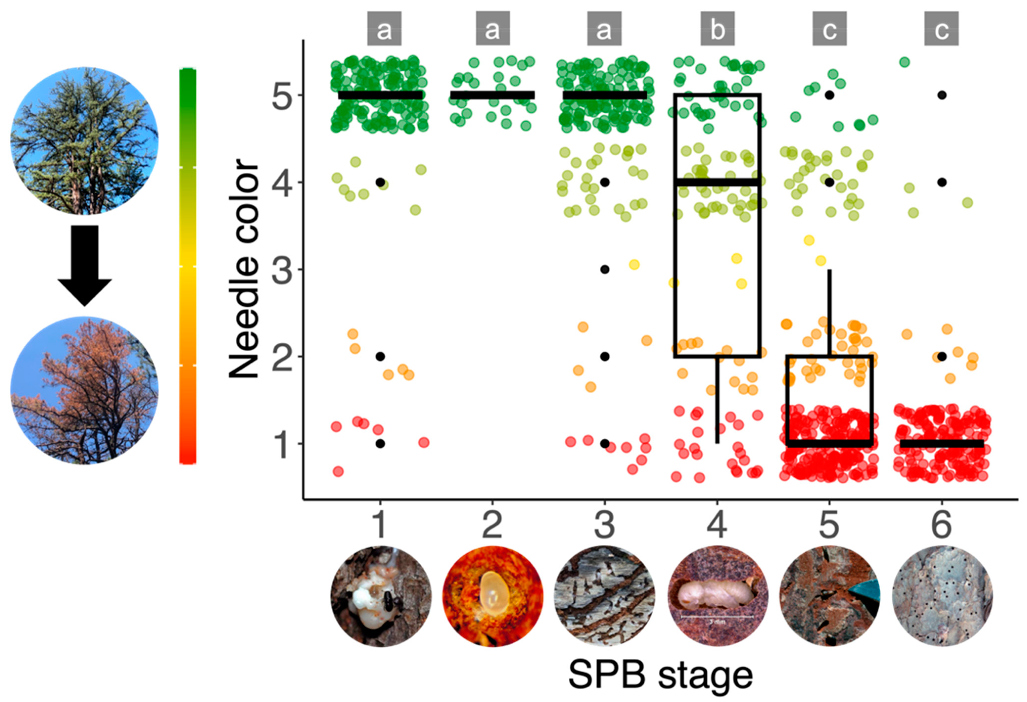
2.2. Ground Data Collection and Analysis

In summer 2022, we sampled all sites during the following intervals: June 6–10; June 20–23; July 5–8; July 19–22; August 1–4; and August 15–18. We visually observed signs of tree decline and then cut a 1 dm² piece of bark to assess brood stage (Figure 2). We cut the bark square at 1.5–2 m at a random cardinal direction. For each attacked tree (n = 310), we recorded diameter at breast height (1.37 m, DBH), tree needle color, percent of needles remaining on the tree, and presence of SPB and other insects on or under the bark. We recorded GPS location using an Arrow 100 GNSS receiver (Eos Positioning Systems; Terrebonne, Quebec, Canada), which maintains sub-meter accuracy even in forested settings by using satellite-based augmentation systems (SBASs). When we cut into the tree to remove a bark sample, we assessed and recorded all SPB stages present. We treated both tree needle color and SPB stage as categorical variables. We categorized tree needle color as (5) green, (4) yellow-green, (3) yellow, (2) reddish-yellow or orange, or (1) red. We categorized SPB stage based on the most advanced development we observed in the 1 dm² bark sample: (1) incipient attack (i.e., SPB adults boring into trees and actively constructing galleries), (2) eggs present in egg niches on either side of galleries, (3) larvae, (4) pupae, (5) callow adults and adults, or (6) evidence of successful SPB development and emergence from the tree with no SPB remaining.

To analyze ground data, we constructed linear mixed effects models using the ‘lme4’ [58] and ‘lmerTest’ [59] packages in R to evaluate differences between SPB stage and tree needle color. Our model included random effects of tree nested within site and sampling date. We used the R package ‘multcomp’ [60] to conduct a post hoc analysis (Tukey’s HSD) and visualized all ground data using ‘ggplot2’ [61].

2.3. UAV Imagery Collection

We collected multispectral imagery from all sites on 6 July 2022. Average temperature during the flights was 29.5 °C with 53% humidity and mostly cloudy skies. Flights were preprogrammed using DJI Ground Station (GS) Pro software version 2.0.17. We flew each site with a DJI Phantom 4 (P4) Multispectral (MS) (Shenzhen, China), flying at the maximum permitted altitude of 120 m and at a speed of 8 m/s, with end and side overlaps of 80%. The DJI P4 MS collects imagery in the following wavelengths: blue (B)—450 nm ± 16 nm; green (G)—560 nm ± 16 nm; red (R)—650 nm ± 16 nm; red edge (RE)—730 nm ± 16 nm; and near-infrared (NIR)—840 nm ± 26 nm. To maximize data collection consistency, the P4 MS uses a solar irradiance sunlight sensor and an internal radiometric calibration based on standard coefficients for each band. We chose to use this UAV model as it is a relatively low-cost and user-friendly option, which makes our methods more practical and potentially adoptable for forest managers.

We flew two flights at Great Hill (4.2 ha and 3.1 ha), two flights at Longwood (1.8 ha and 7.9 ha), and one flight at Brookhaven (14.1 ha) to best capture imagery of the areas where we observed SPB activity in the ground surveys. These flights were short and conducted during consistent wind and sun exposure in order to minimize radiometric changes.

2.4. Image Processing

In Agisoft Metashape version 2.0.0 (Agisoft LLC, St. Petersburg, Russia), we processed our imagery using Unpiloted Aerial System Structure-from-Motion (UAS-SfM) modeling. In our processing workflow (Figure 3), we loaded and aligned all imagery with ‘High Accuracy’ image alignment, then constructed a dense point cloud, a “digital elevation model” (digital surface model), and an orthomosaic for each site and imagery collection date with ‘Ultra High’-quality settings [62,63]. These products are all spatially linked. We visually inspected our orthomosaics to confirm consistency throughout the image. We conducted all analyses on an Intel Xeon E5-2637 v4 CPU with 256 GB of RAM and a NVIDIA Quadro P5000 GPU with 16 GB VRAM.

2.5. Linking Ground Data with UAV Imagery

To accurately link ground data to the corresponding tree crowns as seen in the orthomosaics, we first loaded the orthomosaics into Avenza Maps Pro version 5.2 (Avenza Systems, Inc., Toronto, ON, Canada) on an Apple iPhone 13. Then, using the Arrow 100 GNSS receiver, we visited each tree again in the field and correctly located each tree crown by comparing the GPS point location in Avenza Maps Pro, the shape of the tree crown as seen in the orthomosaic, and the shape of the tree crown in the field. In all, we matched ground and remote sensing data for 138 of 153 trees from the July 2022 flights with high confidence. While linking ground data to imagery can be challenging, we are highly confident in our designations of the locations of these 138 trees due to their crown characteristics, including shape, size, and needle color.

2.6. Individual Tree Detection and Delineation

Our workflow follows that of previous successful work [64]. We detected individual treetops in ArcGIS Pro version 3.1.3 (Esri, Redlands, CA, USA) using the ‘Focal Statistics’ tool. This tool applied a fixed circular window size of 40 cells (0.94 m) on ultra-high-quality canopy height models (CHMs) for each study area. We tested 10 different window sizes, and chose 40 cells to minimize omission error (favoring over-segmentation and minimizing under-segmentation).

We created CHMs by taking the digital surface models produced in our image processing and normalizing these with the 2014 sub-meter New York State LIDAR dataset for Suffolk County, New York [65]. After this normalization, the treetop detection algorithm identifies the highest elevation points that are remaining; each high point is the top of one tree. After treetop detection, we performed marker-controlled watershed segmentation on the CHMs in R [66] using the ‘ForestTools’ package, version 1.0.1 [67]. This step created a segment, or polygon, around each identified treetop in the CHM, effectively delineating the canopy into individual tree crowns. We applied a minimum tree height threshold of 5 m during the segmentation process and then eliminated tree crown segments less than 50 pixels in size for analysis and classification. Lastly, we linked these tree crown segments to the orthomosaics in order to delineate the imagery.

2.7. Object-Based Image Analysis, Classification, and Validation

We calculated spectral, geometric, and textural attributes (n = 32) for each tree segment in Trimble eCognition version 10.2 (Munich, Germany) (

Table 1. Individual tree crown features (n = 32) calculated via eCognition software version 10.2. See Table A1 for spectral indices (n = 20) derived from spectral features.

Geometric Features	Textural Features	Spectral Features
Area (pixels) Asymmetry Border index Compactness Density Length (pixels) Length/width Radius of long ellipsoid Radius of short ellipsoid Roundness Shape index	GLCM * Contrast GLCM Correlation GLCM Dissimilarity GLCM Entropy GLCM Homogeneity GLCM Mean GLDV † Contrast GLDV Entropy GLDV Mean	Brightness HSI intensity Mean blue Mean green Mean red Mean red edge Mean NIR Standard deviation blue Standard deviation green Standard deviation red Standard deviation red edge Standard deviation NIR

* GLCM = Gray-Level Co-Occurrence Matrix. ^† GLDV = Gray-Level Difference Vector

). Using spectral attributes of the imagery, we also calculated 20 spectral indices (Appendix A,

Table A1. Spectral indices (n = 20; alphabetical) calculated from our multispectral imagery.

Spectral Index	Equation	References	Bark Beetle Detection
ARI (Anthocyanin reflectance index)	${\displaystyle \frac{1}{\mathrm{Green}}}-{\displaystyle \frac{1}{\mathrm{RE}}}$	[78]	NA
Blue NDVI	${\displaystyle \frac{\mathrm{NIR}-\mathrm{Blue}}{\mathrm{NIR}+\mathrm{Blue}}}$	[79]	[20,80]
CHLRE (Chlorophyll red edge index)	${\displaystyle \frac{\mathrm{NIR}}{\mathrm{RE}}}-1$	[81]	NA
DVI (Difference vegetation index)	$\mathrm{NIR}-\mathrm{Red}$	[82]	[20]
EVI (Enhanced vegetation index)	${\displaystyle \frac{2.5\times (\mathrm{NIR}-\mathrm{Red})}{\mathrm{NIR}+6\times \mathrm{Red}-7.5\times \mathrm{Blue}+1}}$	[83]	NA
GI (Greenness index)	${\displaystyle \frac{\mathrm{Green}}{\mathrm{Red}}}$	[84]	[12,13]
GLI (Green leaf index)	${\displaystyle \frac{(\mathrm{Green}-\mathrm{Red})-(\mathrm{Green}-\mathrm{Blue})}{2\times \mathrm{Green}+\mathrm{Red}+\mathrm{Blue}}}$	[85]	[7]
Green NDVI	${\displaystyle \frac{\mathrm{NIR}-\mathrm{Green}}{\mathrm{NIR}+\mathrm{Green}}}$	[86]	[7,12]
LCI (Leaf chlorophyll index)	${\displaystyle \frac{\mathrm{NIR}-\mathrm{RE}}{\mathrm{NIR}+\mathrm{Red}}}$	[87]	NA
LIC (Lichtenthaler index)	${\displaystyle \frac{\mathrm{Blue}}{\mathrm{RE}}}$	[88]	[20,21]
MCARI (Modified chlorophyll absorption in reflectance index)	(RE − Red) − 0.2$\times$[(RE − Green) $\times$(RE / Red)]	[77]	NA
NDVI (Normalized difference vegetation index)	${\displaystyle \frac{\mathrm{NIR}-\mathrm{Red}}{\mathrm{NIR}+\mathrm{Red}}}$	[89,90]	[7,18,30,31,80]
NGRDI (Normalized green–red difference index, or GRVI)	${\displaystyle \frac{\mathrm{Green}-\mathrm{Red}}{\mathrm{Green}+\mathrm{Red}}}$	[89]	[7,10,13,18]
PBI (Plant biochemical index)	${\displaystyle \frac{\mathrm{NIR}}{\mathrm{Green}}}$	[11]	[7,11]
PSRI (Plant senescence reflectance index)	${\displaystyle \frac{\mathrm{Red}-\mathrm{Green}}{\mathrm{RE}}}$	[91]	NA
RGI (Red–green ratio)	${\displaystyle \frac{\mathrm{Red}}{\mathrm{Green}}}$	[92]	[31]
RDVI (Re-normalized difference vegetation index)	SQRT(NDVI $\times$ DVI)	[93]	NA
Red Edge NDVI (Also known as NDRE and RENDWI)	${\displaystyle \frac{\mathrm{NIR}-\mathrm{RE}}{\mathrm{NIR}+\mathrm{RE}}}$	[94]	NA
RVI (Ratio vegetation index)	${\displaystyle \frac{\mathrm{NIR}}{\mathrm{Red}}}$	[82]	[20]
TVI (Triangular vegetation index)	60 $\times$ (NIR − Green) − 100 $\times$ (Red − Green)	[95]	NA

). We performed classification using the package ‘randomForest’ [68] in R [66], employing random forest supervised classification algorithms, growing each forest to 1000 trees, and with seven predictors sampled for splitting at each node [69,70]. We also used ‘caTools’ [71] to split our reference data (

Table 2. Reference data sample sizes for each tree class included in our random forest classification.

Class	Reference Sample Size	Percentage of Reference Samples	Balanced Sample Size	Percentage of Balanced Samples
Deciduous	331	34.4%	62	20%
Healthy pine	147	15.3%	62	20%
SPB green attack	62	6.4%	62	20%
SPB visible attack	102	10.6%	62	20%
Dead pine	321	33.3%	62	20%
Total	963	100.0%	310	100%

) into test and training sets before every run, and ‘dplyr’ [72] to summarize algorithm outputs in R. In our initial analysis, we assigned each tree segment to one of five classes: deciduous, dead pine (no needles), healthy pine (no SPB, green needles), SPB green attacks (SPB, green needles), and visible SPB attacks (SPB, ranging from yellow to red needles) (Figure 4).

To maximize classification accuracy, we adjusted several parameters for our random forest algorithms, including the proportion of training and testing data randomly selected from the reference dataset, the number of input features, the number of tree classes, and the proportionality of samples in each tree class. We used three different training/testing data proportions: 45/55, 50/50, and 55/45. We tested four different sets of features: (a) using all 52 features, using the (b) top 15 and (c) top 40 features with the highest mean decrease in the Gini index [73] resulting from the algorithm that included all 52 features, and (d) only including features derived from RGB bands (red, green, and blue bands; effectively removing the benefits of multispectral imagery). In addition to running the algorithm with all five tree classes, we also simulated other forest scenarios we could feasibly encounter by removing some classes: a forest with all pine trees (removing “deciduous”), a forest with all green foliage (removing “dead pine” and “visible SPB attacks”), and a forest with no dead trees (removing “dead pine”). Lastly, we explored how balancing sample sizes within each class would impact model accuracy. The class of interest, SPB green attack, contained the fewest samples (n = 62, Table 2), which is not unusual for a study focused on detection. Thus, we ran the algorithm with 62 randomly chosen samples in each class. This method is known as “balanced random forest” [74]. While balanced random forest classification allowed us to account for unequal sample sizes between our tree classes, this method required us to reduce the overall number of segments included in the classification since we are limited by the number of samples in our rarest class.

In total, we constructed 60 different random forest algorithms, including every combination of training/testing data proportions (3), sampling scenario (5), and sets of features (4). We ran each of the 60 algorithms ten times to assess accuracy, producing 600 error matrices [75,76]. We assessed each of the 60 algorithms by comparing mean accuracy calculated from the ten runs of each algorithm. We then assessed the importance of features in our best-performing algorithms using mean decrease in accuracy and mean decrease in the Gini index. For both of these measures, a larger value indicates that the feature contributes highly to the accuracy of classification—thus, removing that feature would decrease the algorithm’s accuracy. While the mean decrease in the Gini index and mean decrease in accuracy can both be used to assess feature importance, these two metrics are not directly comparable. When we completed feature tuning, we ran our balanced random forest model 100 times and calculated the mean and standard deviation for the following: overall accuracy, producer’s accuracy for each tree class, user’s accuracy for each tree class [75,76], decrease in accuracy for each feature–tree class combination, and decrease in the Gini index for each feature. Producer’s accuracy shows false negatives, also known as errors of omission or Type 2 error; user’s accuracy shows false positives, also known as errors of commission or Type 1 error.

3. Results

3.1. Ground Data

Tree needle color differed significantly based on the SPB stage found within the tree (F = 184; df = 5,829; p < 0.001). Post hoc analysis revealed three groupings that differed statistically (Tukey’s HSD, p < 0.001; Figure 5). Attacked trees exhibited green needles during the initial attack, egg, and larval stages (Stages 1–3 from our methodology). When SPB was pupating (Stage 4), individual trees presented a range of needle colors from green to red, including intermediate colors between green and red. From the beginning of the emergence of the next SPB generation (Stage 5) to the complete absence of all SPB life stages (Stage 6), trees exhibited red needles.

3.2. UAV Data

We collected 6198 images during the flights on 6 July 2022. This imagery has a spatial resolution of <4 cm per pixel. We constructed orthomosaics and digital surface models for each of our three sites.

3.2.1. Individual Tree Detection and Delineation

We assessed the accuracy of our tree detection and delineation (segmentation) using 266 manually drawn reference tree crowns. Overall, we accurately detected 94.6% of the reference tree crowns using a fixed circular window size of 40 cells. As we chose to over-segment rather than under-segment our tree crowns, 40.1% of tree crowns were “true detections” while 54.5% of crowns were over-detected (i.e., were larger than the “true” canopy size as manually delineated); just 5.4% were under-detected.

3.2.2. Classification and Accuracy Assessment

Balanced random forest with five tree classes produced a mean overall accuracy of 78.8 ± 3.2% after 100 runs. We chose to use a 50/50 training/testing data split and only the top 15 features based on hyperparameter tuning (see Section 2.6). Balanced random forest classified deciduous trees with the highest producer’s (89.7 ± 5.6%) and user’s accuracy (94.9 ± 4.3%), while we see lower accuracy for our SPB tree classes (

Table 3. Mean ± sd producer’s accuracy and user’s accuracy from 100 runs of our balanced random forest classification.

Tree Class	Mean Producer’s Accuracy	Mean User’s Accuracy
Deciduous	89.7 ± 5.6%	94.9 ± 4.3%
Healthy pine	87.0 ± 8.7%	82.1 ± 7.4%
SPB green attack	68.3 ± 8.5%	72.1 ± 8.3%
SPB visible attack	65.9 ± 9.1%	62.5 ± 9.8%
Dead pine	85.5 ± 6.2%	83.6 ± 8.6%

). For our class of most interest, SPB green attack, the algorithm achieved 68.3 ± 8.5% producer’s accuracy and 72.1 ± 8.3% user’s accuracy. When examining the error matrix produced from one run of this classification (

Table 4. Example error matrix from one run of our balanced random forest classification using all five classes, a 50/50 training/testing data split, and the top 15 features.

		Reference Data
		Deciduous	Healthy Pine	SPB Green Attack	SPB Visible Attack	Dead Pine	Total	User’s Accuracy
Classified Data	Deciduous	33	0	7	4	0	44	75.0%
	Healthy Pine	0	23	0	1	0	24	95.8%
	SPB Green Attack	0	3	23	3	0	29	79.3%
	SPB Visible Attack	0	0	7	21	2	30	70.0%
	Dead Pine	0	2	0	2	24	28	85.7%
	Total	33	28	37	31	26	155
	Producer’s Accuracy	100%	82.1%	62.2%	67.7%	92.3%		Overall Accuracy 80.0%

), we can attribute most error to the misclassification of SPB-related classes. Because we observed high accuracy in the classification of deciduous trees, we also ran the same balanced random forest algorithm with deciduous trees removed from the dataset. This resulted in similar overall accuracy (mean = 76.9 ± 4.1% after 100 runs), with higher producer’s and user’s accuracy for SPB green attack trees as shown in the example error matrix (

Table 5. Example error matrix from one run of our balanced random forest classification using four classes (removing deciduous trees), a 50/50 training/testing data split, and the top 15 features.

		Reference Data
		Healthy Pine	SPB Green Attack	SPB Visible Attack	Dead Pine	Total	User’s Accuracy
Classified Data	Healthy Pine	26	1	2	0	29	89.7%
	SPB Green Attack	1	25	4	1	31	80.6%
	SPB Visible Attack	2	4	19	5	30	63.3%
	Dead Pine	0	0	3	28	31	90.3%
	Total	29	30	28	34	121
	Producer’s Accuracy	89.7%	83.3%	67.9%	82.4%		Overall Accuracy 81.0%

).

We assessed overall feature importance via mean decrease in the Gini index (Figure 6). The mean of the red band (Mean red) was our most important feature, followed by the standard deviation of the green band (St. dev. green), the standard deviation of the red band (St. dev. red), and modified chlorophyll absorption in reflectance index (MCARI). The standard deviation of the red band was the most important feature for classifying SPB green attack, as seen by the mean decrease in accuracy for this specific class (

Table 6. Mean ± sd decrease in Gini index, and mean ± sd decrease in accuracy for each of our five tree classes from 100 balanced random forest classifications using a 50/50 training/testing data split and the top 15 features. For all data shown here, higher values indicate higher feature importance. The most important feature for each class is designated by bold text. Features with an asterisk (*) require red edge and/or NIR bands. Refer to Appendix A, Table A1, for full description of features.

Feature	Mean Decrease in Accuracy (%)					Mean Decrease in Gini Index
	Deciduous	Healthy Pine	SPB Green Attack	SPB Visible Attack	Dead Pine
Mean red	36.9± 8.1	17.3 ± 4.8	8.4 ± 5.7	11.1 ± 5.0	16.5 ± 4.0	17.1± 3.8
St. dev. green	18.9 ± 4.5	16.5 ± 5.4	16.5 ± 4.4	4.2 ± 4.7	25.6 ± 8.7	14.4 ± 4.0
St. dev. red	6.8 ± 3.9	17.9 ± 5.4	21.9± 5.9	23.4± 7.8	9.0 ± 5.5	12.1 ± 2.4
MCARI *	10.4 ± 3.5	22.3± 4.4	21.2 ± 4.0	3.2 ± 3.2	10.8 ± 3.4	9.9 ± 1.8
ARI *	10.0 ± 2.9	13.7 ± 3.9	8.4 ± 3.6	1.3 ± 4.4	25.9± 6.1	9.5 ± 2.8
St. dev. blue	16.6 ± 5.5	12.0 ± 4.8	8.4 ± 4.0	9.2 ± 4.2	5.3 ± 3.7	8.1 ± 2.4
GLCM entropy	3.4 ± 2.6	14.4 ± 5.3	10.7 ± 5.6	6.9 ± 5.0	11.5 ± 4.9	8.0 ± 2.2
TVI *	9.9 ± 2.7	15.7 ± 2.8	16.2 ± 3.1	4.4 ± 3.3	7.1 ± 2.4	7.1 ± 1.2
LCI *	18.9 ± 5.6	13.3 ± 3.8	2.6 ± 3.6	10.7 ± 4.6	3.6 ± 2.7	7.0 ± 2.0
PBI *	14.3 ± 3.2	12.6 ± 2.6	2.6 ± 2.5	3.4 ± 3.2	13.2 ± 2.8	6.3 ± 1.9
Green NDVI *	14.4 ± 3.2	12.5 ± 2.7	2.6 ± 2.7	3.4 ± 3.3	13.2 ± 2.9	6.2 ± 1.9
Mean green	10.9 ± 2.7	5.4 ± 4.1	6.9 ± 3.7	0.7 ± 3.4	11.3 ± 5.5	5.7 ± 2.5
DVI *	10.9 ± 3.1	9.1 ± 2.7	5.7 ± 1.8	3.0 ± 2.7	8.3 ± 2.5	4.5 ± 1.5
NDVI *	6.0 ± 2.4	8.4 ± 2.2	8.3 ± 2.2	2.3 ± 2.4	7.2 ± 2.4	3.4 ± 0.9
RVI *	6.0 ± 2.2	8.4 ± 2.2	8.6 ± 2.1	2.4 ± 2.2	7.1 ± 2.2	3.4 ± 0.8

); modified chlorophyll absorption in reflectance index (MCARI) was the second most important feature for this class.

4. Discussion

4.1. Ground Data

We sampled SPB brood stage and visually assessed tree needle color for 310 SPB-attacked pitch pines on Long Island, sampling each tree 3.4 times on average between June and August, 2022. Attacked trees typically exhibited green needles until SPB pupation, and by the time we recorded foliage as red in our bi-weekly assessments, SPB had emerged from the tree (Figure 5). Trees classified as “yellow” in our visual assessments were exceedingly rare in our dataset, occurring only six times (<0.6% of sampling events). This supports previous observations by researchers and forestry professionals in SPB outbreaks on Long Island: the needle color of SPB-attacked pitch pines quickly changes from green to red without a distinctive intermediate, yellow stage. It is possible that trees do pass through the yellow stage but that this happens so quickly that it is difficult to detect without more frequent sampling. Also, while we did record intermediate needle colors besides yellow (including “fading green”, “orange”, and other colors that we could not classify as distinctly red, green, or yellow), these intermediate needle colors were associated with later stages of SPB development in the tree: pupation and emergence. These results show that the early detection of SPB-attacked trees is essential for timely management to minimize the impacts of SPB outbreaks.

Our findings also align with some of the literature from the southeastern US, which—despite the dominant green to yellow to red paradigm—suggests that color change is variable and may be decoupled from a precise brood stage. For example, a 1979 field guide for ground checking SPB spots describes that foliage of SPB-attacked trees is “green on most trees containing larvae, but may fade to yellow or turn red before the new generation of beetles emerged from the tree. Foliage color varies greatly by season and among individual trees, so it is not always a good indicator [for this stage]” [52]. Subsequent publications describe tree decline symptoms similarly [49,50]. Thus, it is not clear whether our results indicate tree decline dynamics with respect to SPB attack, or if the conventional wisdom around color change simply represents a useful guide through the range of SPB. We suspect the latter, though it does appear that spatial patterns of attack do differ in northern sites. In either case, there is considerable room for improvement in detection. Our results further support the utility of multi- or hyperspectral SPB detection methods.

4.2. UAV Data

We add the first UAV-based study to the SPB remote sensing literature, and we show that multispectral imagery is valuable for detection of SPB early attack. Balanced random forest classification indicates that the mean reflectance of the red band, standard deviation of the green band, and standard deviation of the red band were the most important spectral features for our overall classification (Figure 6). This result suggests that the amount of variation in green and red reflectance within an individual tree crown segment is useful for classification. These top three features were most important for deciduous trees, SPB green attack, and SPB visible attack (Table 6). Modified chlorophyll absorption in reflectance index (MCARI) was the fourth most important feature, and was the most important for identifying healthy pines. The acanthocyanin reflectance index (ARI) was the fifth most important feature, and was most important for identifying dead pines. While the top three features are all derived from the visible light spectrum, MCARI and ARI require the NIR wavelength. MCARI was the second most important feature for classifying SPB green attack, which is the class we set out to detect. High values of MCARI indicate low chlorophyll levels [77]. This feature suggests that even if trees appear green to the human eye during early SPB attack, chlorophyll production may be decreasing and chlorophyll may be breaking down, decreasing the tree’s capacity for photosynthesis.

Balanced random forest classification produced the highest accuracies when classifying deciduous trees, healthy pine trees, and dead pine trees (Table 3). This is somewhat unsurprising since deciduous trees and dead pine trees are easy to differentiate visibly in our imagery (Figure 4). Healthy pine trees look similar to SPB green attack trees, and this can be seen in the error matrices (Table 4 and Table 5). What is more surprising is the error in classifying SPB green attack vs. SPB visible attack trees. These decline states can be varible, and the classification errors may indicate that the SPB green attack trees have similar spectral reflectances to the SPB visible attack trees—even if they look different to observers in the forest. With additional sampling, these classification errors may be minimized.

Overall, spectral features and spectral indices had a higher mean decrease in the Gini index than textural and geometric features. Over half (9) of the top 15 features require red edge and/or NIR bands (Table 5). The results of our balanced random forest classification suggest that multispectral imagery allows for better classification of SPB early attack than RGB imagery alone.

4.3. Data Gaps, Limitations, and Practical Recommendations

Logistical constraints limited the available sample size for SPB early attack trees. With our ground sampling and UAV sampling crews consisting of different personnel, we had to ensure that the flight occured (1) during peak SPB attack (when the highest number of SPB early attack trees would exist), (2) when our ground sampling crew was in the field (every other week), and (3) when our UAV sampling crew was available. In an ideal world, the sampling crew would include experts in entomology, dendrology, and remote sensing. When this is not feasible, collaboration is key. We prioritized ground surveys and acknowledge that remote sensing is not a replacement for, but rather a complement to, this kind of “boots on the ground” work. While we expected flight scheduling to pose a challenge, we did not anticipate the level of positional precision required to link the ground surveys and UAV data. Initially, we did not use the Arrow 100 GPS unit, instead using a more traditional handheld GPS unit with ±5 m accuracy. The Arrow 100 allows for sub-meter accuracy in optimal conditions. Still, accurately linking ground sampled trees to tree crowns visible in the orthomosaics required the Arrow 100 and simultaneous study of the shape of tree crowns in the field. While GPS location should always be recorded at the time of ground sampling, we recommend that a confirmation of the ground data and aerial imagery link occur during a field site visit after orthomosaics are constructed.

In addition to increasing sample size, future work could include repeated flights to capture changes in reflectance of the same trees over the growing season. This would allow for tracking of individual trees as they decline and for assessment of changes in feature importance. By tracking the decline of many individual trees, we could also study SPB spot growth patterns and increase our understanding of how SPB spots spread on the landscape. We are also curious about the utility of hyperspectral remote sensing in detecting SPB early attack. Our results indicate that NIR and red edge bands contributed to detection of SPB early attack, providing higher accuracy than RGB bands alone. It remains unknown if additional spectral bands would provide significant benefits to this kind of analysis.

While we used an affordable and relatively simple UAV to ensure the practicality of our results, future work can investigate the utility of more advanced UAVs in SPB early attack detection. We acknowledge that the Phantom 4 MS UAV is not the most sophisticated unit available, and its self-calibration process is a source of uncertainty in our work. Some additional uncertainty comes from the geospatial accuracy of the imagery itself. We did not use ground control points because our study sites were forested, and the targets would be difficult to find in this setting. Thus, the vertical accuracy of our digital surface models and canopy height models may be lower than if we had used ground control points. Still, because we link our ground and UAV data by visiting the field with our imagery in hand to match each tree to the imagery, we can conclude that our methodology is sound based on our accuracy assessments: we accurately detected 94.6% of tree crowns in our imagery, and balanced random forest classification achieved 78.8% accuracy overall.

If UAV-based early attack detection of SPB is to be user-friendly, the protocol should use a simple, cost-effective UAV for image collection and freely or widely available software for image processing. We have taken the first step and have tested the efficacy of a cost-effective UAV in this study, and we use some open-access (R) and commonly used (ArcGIS) software. As remote sensing technology continues to evolve, future contributions to the SPB remote sensing literature can utilize new methodologies and tools while building upon the foundation we have created here.

5. Conclusions

We assessed SPB brood stage within attacked trees every two weeks during summer 2022 and linked brood stage to visible tree decline symptoms. Overall, SPB-attacked pitch pine trees remained green until the brood entered the pupal stage. By the time the next generation of SPB had emerged from the tree, foliage was red. Ground results support the need for early attack detection, and UAV results show that multispectral imagery allows for better classification of SPB early attacks than RGB imagery alone. We used a balanced random forest classification with a 50/50 training/testing data split and feature reduction to 15 features to classify trees into one of five classes: deciduous, healthy pine, SPB green attack, SPB visible attack, and dead pine. This random forest classification resulted in 78.8% overall accuracy, with 68.3% producer’s accuracy and 72.1% user’s accuracy for our class of interest, SPB green attack. Remote sensing is a powerful complement to traditional ground surveys, and can provide valuable support for early attack detection. Future studies may consider increasing sample sizes, employing temporal tracking of individual trees via repeated imagery collection, and exploring the use of hyperspectral remote sensing. Our work is a critical first step towards creating a practical remote sensing solution for early attack detection of one of the most economically and ecologically impactful bark beetles in eastern North America.

References

1. Coleman, T.W.; Clarke, S.R.; Meeker, J.R.; Rieske, L.K. Forest Composition Following Overstory Mortality from Southern Pine Beetle and Associated Treatments. Can. J. For. Res. 2008, 38, 1406–1418. [Google Scholar] [CrossRef]
2. Franceschi, V.R.; Krokene, P.; Christiansen, E.; Krekling, T. Anatomical and Chemical Defenses of Conifer Bark against Bark Beetles and Other Pests. New Phytol. 2005, 167, 353–376. [Google Scholar] [CrossRef] [PubMed]
3. Rock, B.N.; Vogelmann, J.E.; Williams, D.L.; Vogelmann, A.F.; Hoshizaki, T. Remote Detection of Forest Damage: Plant Responses to Stress May Have Spectral “Signatures” That Could Be Used to Map, Monitor, and Measure Forest Damage. BioScience 1986, 36, 439–445. [Google Scholar] [CrossRef]
4. Ahern, F.J. The Effects of Bark Beetle Stress on the Foliar Spectral Reflectance of Lodgepole Pine. Int. J. Remote Sens. 1988, 9, 1451–1468. [Google Scholar] [CrossRef]
5. Curran, P.J. Remote Sensing of Foliar Chemistry. Remote Sens. Environ. 1989, 30, 271–278. [Google Scholar] [CrossRef]
6. Horler, D.N.H.; Dockray, M.; Barber, J. The Red Edge of Plant Leaf Reflectance. Int. J. Remote Sens. 1983, 4, 273–288. [Google Scholar] [CrossRef]
7. Huo, L.; Lindberg, E.; Bohlin, J.; Persson, H.J. Assessing the Detectability of European Spruce Bark Beetle Green Attack in Multispectral Drone Images with High Spatial- and Temporal Resolutions. Remote Sens. Environ. 2023, 287, 113484. [Google Scholar] [CrossRef]
8. Honkavaara, E.; Näsi, R.; Oliveira, R.; Viljanen, N.; Suomalainen, J.; Khoramshahi, E.; Hakala, T.; Nevalainen, O.; Markelin, L.; Vuorinen, M.; et al. Using Multitemporal Hyper- and Multispectral UAV Imaging for Detecting Bark Beetle Infestation on Norway Spruce. Int. Arch. Photogramm. Remote Sens. Spat. Inf. Sci. 2020, XLIII-B3-2020, 429–434. [Google Scholar] [CrossRef]
9. Hellwig, F.M.; Stelmaszczuk-Górska, M.A.; Dubois, C.; Wolsza, M.; Truckenbrodt, S.C.; Sagichewski, H.; Chmara, S.; Bannehr, L.; Lausch, A.; Schmullius, C. Mapping European Spruce Bark Beetle Infestation at Its Early Phase Using Gyrocopter-Mounted Hyperspectral Data and Field Measurements. Remote Sens. 2021, 13, 4659. [Google Scholar] [CrossRef]
10. Abdullah, H.; Skidmore, A.K.; Darvishzadeh, R.; Heurich, M. Sentinel-2 Accurately Maps Green-Attack Stage of European Spruce Bark Beetle (Ips typographus, L.) Compared with Landsat-8. Remote Sens. Ecol. Conserv. 2019, 5, 87–106. [Google Scholar] [CrossRef]
11. Abdullah, H.; Skidmore, A.K.; Darvishzadeh, R.; Heurich, M. Timing of Red-Edge and Shortwave Infrared Reflectance Critical for Early Stress Detection Induced by Bark Beetle (Ips typographus, L.) Attack. Int. J. Appl. Earth Obs. Geoinf. 2019, 82, 101900. [Google Scholar] [CrossRef]
12. Bárta, V.; Hanuš, J.; Dobrovolný, L.; Homolová, L. Comparison of Field Survey and Remote Sensing Techniques for Detection of Bark Beetle-Infested Trees. For. Ecol. Manag. 2022, 506, 119984. [Google Scholar] [CrossRef]
13. Klouček, T.; Komárek, J.; Surový, P.; Hrach, K.; Janata, P.; Vašíček, B. The Use of UAV Mounted Sensors for Precise Detection of Bark Beetle Infestation. Remote Sens. 2019, 11, 1561. [Google Scholar] [CrossRef]
14. Fassnacht, F.E.; Latifi, H.; Ghosh, A.; Joshi, P.K.; Koch, B. Assessing the Potential of Hyperspectral Imagery to Map Bark Beetle-Induced Tree Mortality. Remote Sens. Environ. 2014, 140, 533–548. [Google Scholar] [CrossRef]
15. Näsi, R.; Honkavaara, E.; Blomqvist, M.; Lyytikäinen-Saarenmaa, P.; Hakala, T.; Viljanen, N.; Kantola, T.; Holopainen, M. Remote Sensing of Bark Beetle Damage in Urban Forests at Individual Tree Level Using a Novel Hyperspectral Camera from UAV and Aircraft. Urban For. Urban Green. 2018, 30, 72–83. [Google Scholar] [CrossRef]
16. Näsi, R.; Honkavaara, E.; Lyytikäinen-Saarenmaa, P.; Blomqvist, M.; Litkey, P.; Hakala, T.; Viljanen, N.; Kantola, T.; Tanhuanpää, T.; Holopainen, M. Using UAV-Based Photogrammetry and Hyperspectral Imaging for Mapping Bark Beetle Damage at Tree-Level. Remote Sens. 2015, 7, 15467–15493. [Google Scholar] [CrossRef]
17. Safonova, A.; Hamad, Y.; Alekhina, A.; Kaplun, D. Detection of Norway Spruce Trees (Picea abies) Infested by Bark Beetle in UAV Images Using YOLOs Architectures. IEEE Access 2022, 10, 10384–10392. [Google Scholar] [CrossRef]
18. Bárta, V.; Lukeš, P.; Homolová, L. Early Detection of Bark Beetle Infestation in Norway Spruce Forests of Central Europe Using Sentinel-2. Int. J. Appl. Earth Obs. Geoinf. 2021, 100, 102335. [Google Scholar] [CrossRef]
19. Kautz, M.; Feurer, J.; Adler, P. Early Detection of Bark Beetle (Ips typographus) Infestations by Remote Sensing—A Critical Review of Recent Research. For. Ecol. Manag. 2024, 556, 121595. [Google Scholar] [CrossRef]
20. Gao, B.; Yu, L.; Ren, L.; Zhan, Z.; Luo, Y. Early Detection of Dendroctonus valens Infestation with Machine Learning Algorithms Based on Hyperspectral Reflectance. Remote Sens. 2022, 14, 1373. [Google Scholar] [CrossRef]
21. Gao, B.; Yu, L.; Ren, L.; Zhan, Z.; Luo, Y. Early Detection of Dendroctonus valens Infestation at Tree Level with a Hyperspectral UAV Image. Remote Sens. 2023, 15, 407. [Google Scholar] [CrossRef]
22. Zhan, Z.; Yu, L.; Li, Z.; Ren, L.; Gao, B.; Wang, L.; Luo, Y. Combining GF-2 and Sentinel-2 Images to Detect Tree Mortality Caused by Red Turpentine Beetle during the Early Outbreak Stage in North China. Forests 2020, 11, 172. [Google Scholar] [CrossRef]
23. Mckeeman, T. Thermal Remote Sensing of Mountain Pine Beetle Green Attack. Master’s Thesis, University of Calgary, Calgary, AB, Canada, 2022. [Google Scholar]
24. Niemann, K.O.; Quinn, G.; Stephen, R.; Visintini, F.; Parton, D. Hyperspectral Remote Sensing of Mountain Pine Beetle with an Emphasis on Previsual Assessment. Can. J. Remote Sens. 2015, 41, 191–202. [Google Scholar] [CrossRef]
25. Runesson, T. Considerations for Early Remote Detection of Mountain Pine Beetle in Green-Foliaged Lodgepole Pine. Ph.D. Thesis, The University of British Columbia, Vancouver, BC, Canada, 1991. [Google Scholar]
26. Coops, N.C.; Johnson, M.; Wulder, M.A.; White, J.C. Assessment of QuickBird High Spatial Resolution Imagery to Detect Red Attack Damage Due to Mountain Pine Beetle Infestation. Remote Sens. Environ. 2006, 103, 67–80. [Google Scholar] [CrossRef]
27. Lawrence, R.; Labus, M. Early Detection of Douglas-Fir Beetle Infestation with Subcanopy Resolution Hyperspectral Imagery. West. J. Appl. For. 2003, 18, 202–206. [Google Scholar] [CrossRef]
28. Foster, A.C.; Walter, J.A.; Shugart, H.H.; Sibold, J.; Negron, J. Spectral Evidence of Early-Stage Spruce Beetle Infestation in Engelmann Spruce. For. Ecol. Manag. 2017, 384, 347–357. [Google Scholar] [CrossRef]
29. Ciesla, W.M.; Bell, J.C., Jr.; Curlin, J.W. Color Photos and the Southern Pine Beetle. Photogramm. Eng. 1967, 33, 883–888. [Google Scholar]
30. Carter, G.A.; Seal, M.R.; Haley, T. Airborne Detection of Southern Pine Beetle Damage Using Key Spectral Bands. Can. J. For. Res. 1998, 28, 1040–1045. [Google Scholar] [CrossRef]
31. Meng, R.; Gao, R.; Zhao, F.; Huang, C.; Sun, R.; Lv, Z.; Huang, Z. Landsat-Based Monitoring of Southern Pine Beetle Infestation Severity and Severity Change in a Temperate Mixed Forest. Remote Sens. Environ. 2022, 269, 112847. [Google Scholar] [CrossRef]
32. Crosby, M.K.; McConnell, T.E.; Holderieath, J.J.; Meeker, J.R.; Steiner, C.A.; Strom, B.L.; Johnson, C. The Use of High-Resolution Satellite Imagery to Determine the Status of a Large-Scale Outbreak of Southern Pine Beetle. Remote Sens. 2024, 16, 582. [Google Scholar] [CrossRef]
33. Pye, J.M.; Holmes, T.P.; Prestemon, J.P.; Wear, D.N. Economic Impacts of the Southern Pine Beetle. In Southern Pine Beetle II. General Technical Report SRS-140; Coulson, R.N., Klepzig, K.D., Eds.; U.S. Department of Agriculture Forest Service, Southern Research Station: Asheville, NC, USA, 2011; pp. 213–222. [Google Scholar]
34. Hain, F.P.; Duehl, A.J.; Gardner, M.J.; Payne, T.L. Natural History of the Southern Pine Beetle. In Southern Pine Beetle II. General Technical Report SRS-140; Coulson, R.N., Klepzig, K.D., Eds.; U.S. Department of Agriculture Forest Service, Southern Research Station: Asheville, NC, USA, 2011; pp. 13–24. [Google Scholar]
35. Lombardero, M.J.; Ayres, M.P.; Ayres, B.D.; Reeve, J.D. Cold Tolerance of Four Species of Bark Beetle (Coleoptera: Scolytidae) in North America. Environ. Entomol. 2000, 29, 421–432. [Google Scholar] [CrossRef]
36. Tran, J.K.; Ylioja, T.; Billings, R.F.; Régnière, J.; Ayres, M.P. Impact of Minimum Winter Temperatures on the Population Dynamics of Dendroctonus frontalis. Ecol. Appl. 2007, 17, 882–899. [Google Scholar] [CrossRef] [PubMed]
37. Dodds, K.J.; Aoki, C.F.; Arango-Velez, A.; Cancelliere, J.; D’Amato, A.W.; DiGirolomo, M.F.; Rabaglia, R.J. Expansion of Southern Pine Beetle into Northeastern Forests: Management and Impact of a Primary Bark Beetle in a New Region. J. For. 2018, 116, 178–191. [Google Scholar] [CrossRef]
38. Kanaskie, C.R.; Schmeelk, T.C.; Cancelliere, J.A.; Garnas, J.R. New Records of Southern Pine Beetle (Dendroctonus frontalis Zimmermann; Coleoptera: Curculionidae) in New York, New Hampshire, and Maine, USA Indicate Northward Range Expansion. Coleopt. Bull. 2023, 77, 248–251. [Google Scholar] [CrossRef]
39. McGrady, J. Conservation Groups Team Up To Combat Southern Pine Beetle Outbreak. Nantucket Current, 22 August 2023. [Google Scholar]
40. Humphrey, T. Pine Beetle Infestation Invades Island Forests. The Vineyard Gazette, 15 August 2023. [Google Scholar]
41. Lesk, C.; Coffel, E.; D’Amato, A.W.; Dodds, K.; Horton, R. Threats to North American Forests from Southern Pine Beetle with Warming Winters. Nat. Clim. Change 2017, 7, 713–717. [Google Scholar] [CrossRef]
42. Gara, R.I.; Vité, J.P.; Cramer, H.H. Manipulation of Dendroctonus frontalis by Use of a Population Aggregating Pheromone. Contrib. Boyce Thompson Inst. 1965, 23, 55–66. [Google Scholar]
43. Coulson, R.N.; McFadden, B.A.; Pulley, P.E.; Lovelady, C.N.; Fitzgerald, J.W.; Jack, S.B. Heterogeneity of Forest Landscapes and the Distribution and Abundance of the Southern Pine Beetle. For. Ecol. Manag. 1999, 114, 471–485. [Google Scholar] [CrossRef]
44. Ayres, M.P.; Martinson, S.J.; Friedenberg, N.A. Southern Pine Beetle Ecology: Populations within Stands. In Southern Pine Beetle II. General Technical Report SRS-140; Coulson, R.N., Klepzig, K.D., Eds.; U.S. Department of Agriculture Forest Service, Southern Research Station: Asheville, NC, USA, 2011; pp. 75–90. [Google Scholar]
45. Martinson, S.J.; Ylioja, T.; Sullivan, B.T.; Billings, R.F.; Ayres, M.P. Alternate Attractors in the Population Dynamics of a Tree-Killing Bark Beetle. Popul. Ecol. 2013, 55, 95–106. [Google Scholar] [CrossRef]
46. Paine, T.D.; Raffa, K.; Harrington, T. Interactions among Scolytid Bark Beetles, Their Associated Fungi, and Live Host Conifers. Annu. Rev. Entomol. 1997, 42, 179–206. [Google Scholar] [CrossRef]
47. Gara, R.I.; Coster, J.E. Studies on Attack Behavior of Southern Pine Beetle. III Sequence of Tree Infestation within Stands. Contrib. Boyce Thompson Inst. 1968, 24, 77–85. [Google Scholar]
48. Guldin, J.M. Silvicultural Considerations in Managing Southern Pine Stands in the Context of Southern Pine Beetle. In Southern Pine Beetle II. General Technical Report SRS-140; Coulson, R.N., Klepzig, K.D., Eds.; U.S. Department of Agriculture Forest Service, Southern Research Station: Asheville, NC, USA, 2011; pp. 317–352. [Google Scholar]
49. Billings, R.F. Mechanical Control of Southern Pine Beetle Infestations. In Southern Pine Beetle II. General Technical Report SRS-140; Coulson, R.N., Klepzig, K.D., Eds.; U.S. Department of Agriculture Forest Service, Southern Research Station: Asheville, NC, USA, 2011; pp. 399–413. [Google Scholar]
50. Swain, K.M.; Remion, M.C. Direct Control Methods for the Southern Pine Beetle; U.S. Department of Agriculture: Washington, DC, USA, 1981.
51. Cancelliere, J. Effects of Winter Cut-and-Leave Suppression on SPB Overwintering Success; New York Department of Environmental Conservation: Albany, NY, USA, 2018.
52. Billings, R.F.; Herbert, A., III. A Field Guide for Ground Checking Southern Pine Beetle Spots; Agriculture Handbook No. 558; United States Department of Agriculture, Combined Forest Pest Research and Development Program: Washington, DC, USA, 1979.
53. Gifford, N.A.; Deppen, J.M.; Bried, J.T. Importance of an Urban Pine Barrens for the Conservation of Early-Successional Shrubland Birds. Landsc. Urban Plan. 2010, 94, 54–62. [Google Scholar] [CrossRef]
54. Bried, J.T.; Patterson, W.A.; Gifford, N.A. Why Pine Barrens Restoration Should Favor Barrens over Pine. Restor. Ecol. 2014, 22, 442–446. [Google Scholar] [CrossRef]
55. Kanaskie, C.R.; Dodds, K.J.; Stephen, F.M.; Garnas, J.R. Southern Pine Beetle (Coleoptera: Curculionidae) and Its Associated Insect Community: Similarities and Key Differences between Northeastern and Southeastern Pine Forests. Environ. Entomol. 2024, 53, 143–156. [Google Scholar] [CrossRef] [PubMed]
56. Billings, R.F.; Ward, J.D. How to Conduct a Southern Pine Beetle Aerial Detection Survey; Circular-Texas Forest Service: Lufkin, TX, USA, 1984. [Google Scholar]
57. Billings, R.F. Aerial Detection, Ground Evaluation, and Monitoring of the Southern Pine Beetle: State Perspectives. In Southern Pine Beetle II. USDA Forest Service Southern Research Station Gen. Tech Rep. SRS-140; Coulson, R.N., Klepzig, K.D., Eds.; U.S. Department of Agriculture Forest Service, Southern Research Station: Asheville, NC, USA, 2011; pp. 245–261. [Google Scholar]
58. Bates, D.; Mächler, M.; Bolker, B.; Walker, S. Fitting Linear Mixed-Effects Models Using Lme4. J. Stat. Softw. 2015, 67, 1–48. [Google Scholar] [CrossRef]
59. Kuznetsova, A.; Brockhoff, P.B.; Christensen, R.H.B. lmerTest Package: Tests in Linear Mixed Effects Models. J. Stat. Softw. 2017, 82, 1–26. [Google Scholar] [CrossRef]
60. Hothorn, T.; Bretz, F.; Westfall, P.; Heiberger, R.M.; Schuetzenmeister, A.; Scheibe, S. Multcomp: Simultaneous Inference in General Parametric Models. 2023. Available online: https://cran.r-project.org/web/packages/multcomp/index.html (accessed on 14 July 2024).
61. Wickham, H.; Chang, W.; Henry, L.; Pedersen, T.L.; Takahashi, K.; Wilke, C.; Woo, K.; Yutani, H.; Dunnington, D.; van den Brand, T. Ggplot2: Create Elegant Data Visualisations Using the Grammar of Graphics. 2023. Available online: https://cran.r-project.org/web/packages/ggplot2/index.html (accessed on 14 July 2024).
62. Fraser, B.T.; Bunyon, C.L.; Reny, S.; Lopez, I.S.; Congalton, R.G. Analysis of Unmanned Aerial System (UAS) Sensor Data for Natural Resource Applications: A Review. Geographies 2022, 2, 303–340. [Google Scholar] [CrossRef]
63. Fraser, B.T.; Congalton, R.G. Issues in Unmanned Aerial Systems (UAS) Data Collection of Complex Forest Environments. Remote Sens. 2018, 10, 908. [Google Scholar] [CrossRef]
64. Fraser, B.T.; Congalton, R.G. Estimating Primary Forest Attributes and Rare Community Characteristics Using Unmanned Aerial Systems (UAS): An Enrichment of Conventional Forest Inventories. Remote Sens. 2021, 13, 2971. [Google Scholar] [CrossRef]
65. OCM Partners. 2014 USGS CMGP Lidar: Post Sandy (Long Island, NY). Available online: https://www.fisheries.noaa.gov/inport/item/49890 (accessed on 14 July 2024).
66. R Core Team. R: A Language and Environment for Statistical Computing; R Foundation for Statistical Computing: Vienna, Austria, 2023. [Google Scholar]
67. Plowright, A. Package ForestTools: Tools for Analyzing Remote Sensing Forest Data. 2024. Available online: https://cran.r-project.org/web/packages/ForestTools/index.html (accessed on 14 July 2024).
68. Breiman, A.; Cutler, A.; Liaw, A.; Wienner, M. randomForest: Breiman and Cutler’s Random Forests for Classification and Regression. 2022. Available online: https://cran.r-project.org/web/packages/randomForest/index.html (accessed on 14 July 2024).
69. Breiman, L. Random Forests. Mach. Learn. 2001, 45, 5–32. [Google Scholar] [CrossRef]
70. Maxwell, A.E.; Warner, T.A.; Fang, F. Implementation of Machine-Learning Classification in Remote Sensing: An Applied Review. Int. J. Remote Sens. 2018, 39, 2784–2817. [Google Scholar] [CrossRef]
71. Tuszynski, J. caTools: Tools: Moving Window Statistics, GIF, Base64, ROC AUC, Etc. 2021. Available online: https://cran.r-project.org/web/packages/caTools/index.html (accessed on 14 July 2024).
72. Wickham, H.; François, R.; Henry, L.; Müller, K.; Vaughan, D.; Posit Software, PBC. Dplyr: A Grammar of Data Manipulation. 2023. Available online: https://cran.r-project.org/web/packages/dplyr/index.html (accessed on 14 July 2024).
73. Han, H.; Guo, X.; Yu, H. Variable Selection Using Mean Decrease Accuracy and Mean Decrease Gini Based on Random Forest. In Proceedings of the 2016 7th IEEE International Conference on Software Engineering and Service Science (ICSESS), Beijing, China, 26–28 August 2016; pp. 219–224. [Google Scholar]
74. Chen, C.; Liaw, A.; Beiman, L. Using Random Forest to Learn Inbalanced Data; University of California Berkeley: Berkeley, CA, USA, 2004; p. 12. [Google Scholar]
75. Congalton, R.G. A Review of Assessing the Accuracy of Classifications of Remotely Sensed Data. Remote Sens. Environ. 1991, 37, 35–46. [Google Scholar] [CrossRef]
76. Congalton, R.G.; Green, K. Assessing the Accuracy of Remotely Sensed Data: Principles and Practices, 3rd ed.; CRC Press: Boca Raton, FL, USA, 2019; ISBN 978-0-429-62935-8. [Google Scholar]
77. Daughtry, C.S.T.; Walthall, C.L.; Kim, M.S.; de Colstoun, E.B.; McMurtrey, J.E., III. Estimating Corn Leaf Chlorophyll Concentration from Leaf and Canopy Reflectance. Remote Sens. Environ. 2000, 74, 229–239. [Google Scholar] [CrossRef]
78. Gitelson, A.A.; Merzlyak, M.N.; Chivkunova, O.B. Optical Properties and Nondestructive Estimation of Anthocyanin Content in Plant Leaves. Photochem. Photobiol. 2001, 74, 38–45. [Google Scholar] [CrossRef]
79. Blackburn, G.A. Spectral Indices for Estimating Photosynthetic Pigment Concentrations: A Test Using Senescent Tree Leaves. Int. J. Remote Sens. 1998, 19, 657–675. [Google Scholar] [CrossRef]
80. Klouček, T.; Modlinger, R.; Zikmundová, M.; Kycko, M.; Komárek, J. Early Detection of Bark Beetle Infestation Using UAV-Borne Multispectral Imagery: A Case Study on the Spruce Forest in the Czech Republic. Front. For. Glob. Change 2024, 7, 1215734. [Google Scholar] [CrossRef]
81. Gitelson, A.A.; Keydan, G.P.; Merzlyak, M.N. Three-Band Model for Noninvasive Estimation of Chlorophyll, Carotenoids, and Anthocyanin Contents in Higher Plant Leaves. Geophys. Res. Lett. 2006, 33, L11402. [Google Scholar] [CrossRef]
82. Zhu, Y.; Yao, X.; Tian, Y.; Liu, X.; Cao, W. Analysis of Common Canopy Vegetation Indices for Indicating Leaf Nitrogen Accumulations in Wheat and Rice. Int. J. Appl. Earth Obs. Geoinf. 2008, 10, 1–10. [Google Scholar] [CrossRef]
83. Liu, H.Q.; Huete, A. A Feedback Based Modification of the NDVI to Minimize Canopy Background and Atmospheric Noise. IEEE Trans. Geosci. Remote Sens. 1995, 33, 457–465. [Google Scholar] [CrossRef]
84. Smith, R.C.G.; Adams, J.; Stephens, D.J.; Hick, P.T. Forecasting Wheat Yield in a Mediterranean-Type Environment from the NOAA Satellite. Aust. J. Agric. Res. 1995, 46, 113–125. [Google Scholar] [CrossRef]
85. Louhaichi, M.; Borman, M.M.; Johnson, D.E. Spatially Located Platform and Aerial Photography for Documentation of Grazing Impacts on Wheat. Geocarto Int. 2001, 16, 65–70. [Google Scholar] [CrossRef]
86. Gitelson, A.A.; Kaufman, Y.J.; Merzlyak, M.N. Use of a Green Channel in Remote Sensing of Global Vegetation from EOS-MODIS. Remote Sens. Environ. 1996, 58, 289–298. [Google Scholar] [CrossRef]
87. Yu, R.; Luo, Y.; Zhou, Q.; Zhang, X.; Wu, D.; Ren, L. Early Detection of Pine Wilt Disease Using Deep Learning Algorithms and UAV-Based Multispectral Imagery. For. Ecol. Manag. 2021, 497, 119493. [Google Scholar] [CrossRef]
88. Lichtenthaler, H.K.; Lang, M.; Sowinska, M.; Heisel, F.; Miehé, J.A. Detection of Vegetation Stress Via a New High Resolution Fluorescence Imaging System. J. Plant Physiol. 1996, 148, 599–612. [Google Scholar] [CrossRef]
89. Tucker, C.J. Red and Photographic Infrared Linear Combinations for Monitoring Vegetation. Remote Sens. Environ. 1979, 8, 127–150. [Google Scholar] [CrossRef]
90. Rouse, J.W.; Haas, R.H.; Schell, J.A.; Deering, D.W. Monitoring Vegetation Systems in the Great Plains with ERTS. In Proceedings of the Third ERTS-1 Symposium, Washington, DC, USA, 10–14 December 1973; NASA SP-351. National Aeronautics and Space Administration: Washington, DC, USA, 1974; pp. 309–317. [Google Scholar]
91. Merzlyak, M.N.; Gitelson, A.A.; Chivkunova, O.B.; Rakitin, V.Y. Non-Destructive Optical Detection of Pigment Changes during Leaf Senescence and Fruit Ripening. Physiol. Plant. 1999, 106, 135–141. [Google Scholar] [CrossRef]
92. de Santos, I.C.L.; dos Santos, A.; Oumar, Z.; Soares, M.A.; Silva, J.C.C.; Zanetti, R.; Zanuncio, J.C. Remote Sensing to Detect Nests of the Leaf-Cutting Ant Atta sexdens (Hymenoptera: Formicidae) in Teak Plantations. Remote Sens. 2019, 11, 1641. [Google Scholar] [CrossRef]
93. Roujean, J.-L.; Breon, F.-M. Estimating PAR Absorbed by Vegetation from Bidirectional Reflectance Measurements. Remote Sens. Environ. 1995, 51, 375–384. [Google Scholar] [CrossRef]
94. Iordache, M.-D.; Mantas, V.; Baltazar, E.; Pauly, K.; Lewyckyj, N. A Machine Learning Approach to Detecting Pine Wilt Disease Using Airborne Spectral Imagery. Remote Sens. 2020, 12, 2280. [Google Scholar] [CrossRef]
95. Broge, N.H.; Leblanc, E. Comparing Prediction Power and Stability of Broadband and Hyperspectral Vegetation Indices for Estimation of Green Leaf Area Index and Canopy Chlorophyll Density. Remote Sens. Environ. 2001, 76, 156–172. [Google Scholar] [CrossRef]
Figure 1. Maps of study sites on Long Island, New York. Each site is represented by a yellow circle. At the left, we show part of one of the orthomosaics.
Remotesensing 16 02608 g001
Figure 2. We removed a 1 dm2 piece of bark from each attacked tree during each sampling interval to assess southern pine beetle brood stage. The bark sample in this photograph contained mid–late-stage larvae.
Remotesensing 16 02608 g002
Figure 3. Flowchart diagram of our methodology from data collection to random forest classification and accuracy assessment (created via lucid.app).
Remotesensing 16 02608 g003
Figure 4. Examples of each of our five tree segment classes in our imagery. Southern pine beetle (SPB) green attack, also known as early attack, is our class of most interest.
Remotesensing 16 02608 g004
Figure 5. The relationship between the dominant SPB stage present and tree canopy color in ground-assessed trees. We segmented the SPB life cycle on or within a tree into six stages along the x-axis: (1) initial attack, (2) eggs, (3) larvae, (4) pupae, (5) emergence, and (6) complete vacation of the tree by SPB. As the SPB life cycle progresses, tree needle color generally fades from green (5) to red (1) along the y-axis. Letters indicate statistically significant groups (Tukey’s HSD, p < 0.001). [Tree images and SPB Stage 3 (larvae), CRK. Other SPB life stage images downloaded from www.ForestryImages.org under Creative Commons Attribution 3.0 License: 1, image 5432995 (Erich G. Vallery, USDA Forest Service–SRS-4552, www.Bugwood.org); 2, image 0284025 (USDA Forest Service, www.Bugwood.org); 4, image 5433005 (Erich G. Vallery, USDA Forest Service–SRS-4552, www.Bugwood.org); 5, image 0745057 (Erich G. Vallery, USDA Forest Service–SRS-4552, www.Bugwood.org); 6, image 2108027 (Ronald F. Billings, Texas A&M Forest Service, www.Bugwood.org)].
Remotesensing 16 02608 g005
Figure 6. We assessed feature importance via mean decrease in Gini index for our balanced random forest classification using 50/50 training/testing data split and top 15 features. Error bars show standard deviation. Higher values indicate higher feature importance. Refer to Appendix A, Table A1, for full description of features.
Remotesensing 16 02608 g006