Abstract
Clear-air echo studies are usually based on isotropic turbulence theory. But the theory has been considered incomplete by modern turbulence theory. The intermittence of turbulence can reveal obvious shortcomings in the existing studies of clear-air echoes. The mechanism of clear-air echo scattering needs to be supplemented. This paper introduces the troposcatter theory, normally used in over-the-horizon communication, to fill the gap left by Bragg scattering. By treating radar as a self-transmitted and self-received device, the equivalent transmission loss of weather radar is established and compared with the recommendations of the Radiocommunication Sector of the International Telecommunication Union (ITU-R). The results show that the S-band radar transmission loss aligns with ITU-R recommendations. There is also a linear regression relationship between the radar transmission loss and height, which conforms to the troposcatter theory. This means that the theory of troposcatter scattering is a supplement to the theory of Bragg scattering. Tropospheric scattering can be thought of as general Bragg scattering. Meanwhile, based on ITU-R recommendations, this study also provides a new way for the recognition of biological echoes.
1. Introduction
Clear-air echoing is an interesting phenomenon that can be observed using weather radar from a region of the atmosphere without any detectable meteorological scatterers, such as clouds or precipitation. Since the deployment of weather radar after World War II, a vast clear-air echo area has been observed every night during the flood season [1,2]. It is widely acknowledged that the scattering of clear-air echoes at centimeter wavelengths is predominantly governed by two mechanisms: Bragg scattering resulting from turbulent inhomogeneities and biological scattering resulting from insects and birds [3]. However, clear-air turbulence echoes have been neglected in research for a long time, because some researchers do not accept that clear-air echoes can be caused by turbulence and believe that bio-particle scattering is the dominant cause.
Clear-air echoes, especially S-band echoes, have predominantly been attributed to bio-particle scattering because of two pieces of evidence: isotropic turbulence and Bragg scattering. Isotropic turbulence theory was introduced in Kolmogorov’s research. Kolmogorov posited that the properties of turbulence are homogeneous and isotropic, which implies that the intensity of turbulence scattering in the horizontal and vertical planes is consistent [4]. Therefore, if turbulence were the cause of the echo, the differential reflectivity, , would be zero. Additionally, by utilizing the formula for Bragg scattering, the value of the atmospheric structure constant can be calculated from the radar reflectivity factor. However, the structure constant, , calculated from clear-air echoes, surpasses the upper range of observed values. Hence, as the current atmospheric scattering theory cannot provide evidence that turbulence causes clear-air echoes, researchers tend to attribute them to biological activities. However, many studies do not consider the fact that these two pieces of evidence are flawed.
Much research has revealed the extensive existence of non-Kolmogorov turbulence. Batchelor and Townsend were the first to observe the uneven distribution of turbulence and its energy dissipation over space, with intermittent velocity gradients increasing as the Reynolds number increased [5]. Siggia conducted numerical simulations and discovered that a small region of space accounted for 95% of the energy dissipation [6]. Consortini’s team demonstrated the presence of turbulent anisotropy using laser beams in laboratory experiments [7]. Kolmogorov’s theory was found to be incomplete in describing atmospheric statistics properly, particularly in segments of the troposphere and stratosphere [8]. The above findings suggest that non-Kolmogorov turbulence plays a significant role in atmospheric dynamics. Thus, clear-air echoes can have a non-zero according to non-Kolmogorov turbulence.
Several experimental campaigns have also investigated the turbulent air anisotropy in the real atmosphere. One experimental study involved a laser beam propagating horizontally through the near-ground atmosphere, and showed that the intensity correlation function captures the anisotropic turbulence information, corresponding to the refractive index anisotropy ellipse of atmospheric fluctuations [9]. A similar measurement campaign was used to obtain the intensity covariance function of a propagating plane wave and showed that the anisotropy ratio ranged from 0.6/1 to 1/0.6 at different times, where the magnitudes of and affected the horizontal and vertical strength of turbulence through the refractive index structure constant [10]. The results of these measurements suggest that the value of turbulent air can vary over a wide range of the actual atmosphere. Based on the studies mentioned above, this range is between −2 dB and 2 dB. This explains the non-zero differential reflectivity of clear-air turbulence echoes. However, Bragg scattering, as another piece of evidence, has not been updated since it was first introduced.
In 1969, Ottersten summarized progress in the field of radar backscattering from refractive index irregularities in clear air and described their relationship to atmospheric structure and turbulence [11]. His study showed that the relationship between microstructure and atmospheric mean fields can be illustrated for a simplified situation in the stable regime, from which it can be concluded that strong clear-air turbulence will be associated with zones of increased refractive index variability and enhanced radar returns. Four years later, his team summarized and discussed the experimental progress made since 1969, showing how the echo patterns obtained could be used to interpret multiple layering, gravity waves, internal fronts, and the details of dynamic instability and turbulence generation in stably stratified shear layers [12]. This research laid the theoretical foundations of Bragg clear-air scattering. Bragg scattering has also been discussed in detail in some studies, but there has been no substantial update of the theory. However, the field of wireless communications, which is similar to that of radar, proposes a new mechanism.
In respect of communication, tropospheric scattering (also known as troposcatter) has been suggested as an efficient propagation method by the Radiocommunication Sector of the International Telecommunication Union. This is the mechanism by which microwave radio systems inadvertently achieve beyond-the-horizon communications [13]. According to the currently accepted theory of tropospheric scattering, information transfer is the result of the combination of the following three models [14]: the reflective layer model [15], scattering from turbulence [16], and reflections from an exponential atmosphere [17]. By comparing tropospheric scattering with radar theories, it is clear that Bragg scattering and Fresnel scattering involve backward scattering forms of turbulent scattering and reflections from an exponential atmosphere, respectively. However, little attention has been paid to the connection between tropospheric scattering and clear-air echoes. The reflecting layer model, one of the three mechanisms of tropospheric scattering, has been forgotten in the study of clear-air echoes. This has led to a large number of studies based on an incomplete scattering theory of the clear-air echo.
Researchers generally base their studies of meteorological clear-air echoes exclusively on Bragg scattering and isotropic turbulence. Mueller and Larkin argued that scattering is due to refractive index fluctuations on a scale of one-half the wavelength due to isotropic turbulence [18]. Gossard stated in his book that observed clear-air echoes are much larger than the value that the atmospheric structure constant can provide, if only conventional Bragg scattering is considered [19]. Wilson et al. performed radar reflectivity comparisons of clear-air echoes in Florida and Colorado at wavelengths of 3, 5, and 10 cm, and concluded that insects are primarily responsible for the clear-air echoes in the mixed boundary layer [2]. They also concluded that at and above the top of the well-mixed boundary layer, Bragg scattering dominates and is frequently observed in the S-band. However, although earlier studies have suggested that their conclusions apply only to isotropic turbulence, the statistical results of many studies do not take into account the effects produced by non-isotropic turbulence because no new theories have been proposed. Thus, this study focuses on the relationship between radar clear-air echoes and tropospheric scattering.
In this study, we introduce the theory of troposcatter from over-the-horizon communication into atmospheric physics. The aim is to extend the set of scattering mechanisms of turbulence. Radar is treated as a self-transmitting and self-receiving wireless communication system, which allows us to explain troposcatter in the atmosphere. This approach provides a new perspective on the study of clear-air scattering in atmospheric physics. Section 2 provides a brief overview of radar and troposcatter, along with a short introduction to Bragg scattering. Section 3 describes the instruments and their function, followed by a discussion of the characteristics of clear-air echoing in troposcatter in Section 4. Section 5 introduces a possible application in biological monitoring and presents the existing drawbacks of the study. Lastly, Section 6 presents a summary of the article.
2. Concepts and Theory
2.1. Radar Range Equations
Radar relies on backscattering to generate a detectable echo from a target. Weather radar emits radio energy from a transmitting antenna and propagates the radio wave outward in a narrow beam through the atmosphere. In the path of the beam, a small portion of the reflected and scattered energy travels back and is intercepted by the receiving antenna. The radar range equation is the foundation of radar remote sensing and describes the physical dependencies on the transmission power and how the wave propagates up to receiving the echo signals. To express the power of the echo signal as a function of the distance to the target, and the target radar reflectivity , the equation can be written as follows:
where is the received power, is the peak power transmitted by the radar, is the gain of the antenna, denotes the antenna beamwidth, is the pulse length of the transmitted signal, and is the wavelength. The reflectivity is the sum of radar cross section per unit volume.
In radar meteorology, the reflectivity factor ( hereafter) is a common term for the received power because it equals the sum of the sixth-power of the diameters of the water drops in a unit volume of space, which means establishing the relationship between the precipitation intensity and the signal power. For Rayleigh scattering, the reflectivity is expressed as follows [2,20]:
where is the wavelength; is often taken to be 0.93 for water as a dielectric constant. Equation (2) is derived only for Rayleigh scattering, considering for water. During actual atmospheric precipitation, there is not only Rayleigh scattering but also Mie scattering, and the precipitation phase is more complex.
2.2. Bragg Scattering
Kolmogorov introduced a structure function to describe the structure of atmospheric turbulence [21,22]. Based on Kolmogorov’s theory, Ottersten provided a link between , , and (the refractive index structure constant), which is called Bragg scattering as shown in Equation (3) [3]:
Bragg scattering is caused by turbulent inhomogeneities with sizes around one-half of [23,24,25,26,27]. in respect of Bragg scattering is given in Equation (4) [2]:
Equation (4) establishes the relationship between the reflectivity factor and the atmospheric refractive index structure constant . By using Equation (4), the structure constant of the atmosphere can be calculated when Bragg scattering is caused by turbulence. The value of clear-air echoes is usually distributed between 10 dBZ and 20 dBZ, but the calculated value of is larger than , which is far from the observable maximum value [2,19]. This is why some scholars believe that clear-air echoes cannot be caused by Bragg scattering.
Notably, Equation (4), like Equation (2), is highly simplified, and the effects of numerous factors need to be considered when using radar reflectivity factors to accurately calculate the structural constants. However, since the values calculated from the values of clear-air echoes are several magnitudes away from the actual observed , Wilson’s view is overwhelmingly accepted. As a result, this has led a considerable number of scholars to deny, based on Wilson’s view, that clear-air echoes are produced by Bragg scattering.
2.3. Tropospheric Scattering
2.3.1. Scattering Models
Troposcatter refers to the scattering of signals caused by atmospheric irregularities in the troposphere. It has been recognized as a promising method for wireless communication beyond the line of sight by the Radiocommunication Sector of the International Telecommunication Union (ITU-R) [13]. Troposcatter has emerged as a promising candidate for communication beyond line-of-sight because it has important features including security and low transmission delay [28]. Since the 1950s, the characteristics of troposcatter propagation and its propagation mechanism have been detailed in numerous studies. Generally, three main theories have been proposed: turbulent incoherent scattering theory [15], coherent reflection by stable layers theory [16], and incoherent reflection by irregular layers theory [17]. The theory of incoherent scattering due to turbulence posits that the movement and variation of turbulent vortices create inhomogeneity with a continually changing dielectric permittivity and become sources of receiving signals.
Coherent reflection by stable layers theory is based on the assumption that the atmosphere can be divided into a series of thin layers that reflect incident radio waves. In the theory of incoherent reflection by irregular layers, there are irregular layers in the troposphere formed by atmospheric convection. These layers have a wildly fluctuating refractive index gradient and reflect the radio waves from these irregular layer boundaries. It is obvious that incoherent scattering due to turbulence is essentially consistent with Bragg scattering, while stable layer reflection is similar to Fresnel reflection, which can be observed using UHF and VHF radars.
It is generally accepted that troposcatter is the result of a combination of these three models. Therefore, the scattering of troposcatter can generate stronger signals than the scattering caused by a single model alone. A previous study noted that the combination of these three models has the same form of scattering cross-section, , and of the troposcatter can be written as follows [14]:
where , , and are constants and are measured experimentally; is the dielectric constant; is the height; and is the glancing angle. In fact, since radar mainly detects the backscattered signal, the value of the grazing angle is fixed (the grazing angle is a right angle). Therefore, the remaining terms other than wavelength can be regarded as constant terms affected by the atmosphere, and Equation (5) can be rewritten as
where
Notably, when equals and equals , Equation (6) for tropospheric scattering and Equation (3) for Bragg scattering are consistent. Thus, tropospheric scattering can be regarded as a general theory of Bragg scattering.
It is known that troposcatter is a phenomenon of signal scattering caused by atmospheric irregularities in the troposphere. The turbulent air mass is highly irregular and is constantly changing in terms of its shape, location, and orientation. As a result, electromagnetic waves are scattered (and reflected) in all directions. For this reason, researchers refer to this communication mode as tropospheric “scattering” rather than tropospheric “refraction” or tropospheric “reflection”.
A visual schematic is shown in Figure 1. The wide radar beam radiates the inhomogeneous turbulent mass. Because the air mass is small and heterogeneous, the radar waves are reflected and scattered in all directions at the same time by different reflective surfaces of the same air mass and by reflective surfaces of different air masses. As a result, although there are some differences in their reflectivity, both tropospheric forward and backward scattering occur simultaneously.
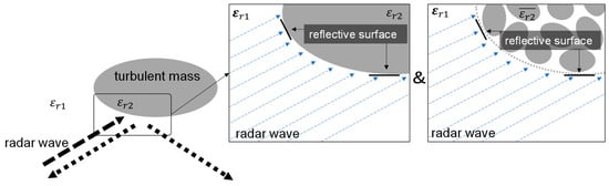
Figure 1.
Reflection and scattering concept diagram of tropospheric scattering. and is the dielectric constant of different air mass, and is the mean of the dielectric constant. Differences in the refractive index of a single air mass from its surroundings can lead to the reflective surface. And the average refractive index of multiple air masses can also result in reflective surfaces due to differences in refractive index with other air masses.
2.3.2. Transmission Loss
In order to employ the troposcatter phenomenon for over-the-horizon communication, it is crucial to establish a suitable troposcatter propagation model that can accurately predict transmission loss. Since the 1980s, the ITU-R has collected measurement data worldwide and provided recommendations for standardized troposcatter loss prediction methods [13].
In this section, we briefly summarize the ITU-R’s recommendations, and for more detail, readers can refer to the ITU-R’s website (https://www.itu.int/rec/R-REC-P/en, accessed on 29 July 2023). In recommendation ITU-R P.617, the average annual transmission loss is written as [29]
where
where and are the transmitter and receiver horizon angles, respectively, and
with the remaining parameters listed in Table 1.

Table 1.
Principal parameters.
In Equation (8), is a conversion factor for non-exceedance percentages, , other than 50% from
where is the conversion factor for = 90%, and in most regions of China, is
The coefficient denotes the non-exceedance percentage of time. According to the ITU-R recommendations, the values of are 50 and 91.82 for values of 50 and 99, respectively.
The ITU-R continuously updates the current internationally agreed, general-purpose, wide-range, terrestrial propagation model that is known as ITU-R P.2001 [30]. The propagation model is used to predict terrestrial propagation loss due to both signal enhancements and fading over the time range 0% to 100% of an average year. It covers the frequency range from 30 MHz to 50 GHz and distances from 3 km to 1000 km. The prediction of troposcatter transmission loss is described as follows:
where
Although is the same as as in Equation (15), is given by:
2.3.3. Radar Transmission Loss
The received signal in radar is, essentially, the unmodulated carrier wave transmitted by the radar itself. Remote sensing methods using radar and wireless communication share similarities in the way they work. However, radar places greater emphasis on changes in the echo of the carrier due to the impact of the wireless channel, while communication focuses on maintaining the quality of the transmitted signals. To match the troposcatter transmission loss with the radar reflectivity factor, the transmission loss of weather radar, , is expressed as follows:
By substituting Equations (1) and (2), can be defined simply as
Thus, using in Equation (22), the troposcatter transmission loss and the radar transmission loss can be linked to radar parameters and the radar reflectivity factor. However, there is an associated issue. Because the receiving and transmitting ends of wireless communication are independent, the grazing angle is half of the scattering angle. Radar is an integrated transmitter and receiver device that only receives backscattered signals (regardless of multiple scattering and multipath effects). Therefore, to compare the transmission loss of radar with that of wireless communication beyond the line of sight, a calibration coefficient is needed to correct for the difference in intensities between the grazing direction and backscatter.
It is well known that when an electric wave is incident from a medium with dielectric constant to an infinite interface with a medium of dielectric constant , the Fresnel reflection coefficient, , can be simplified as follows:
where is the elevation of the radar beam (i.e., the same as the glancing angle).
Then, referring to Equation (24), the calibration coefficient, , can be defined as
Thus, the radar equivalent transmission loss (, transmission loss in short hereafter) is as follows:
3. Instruments and Data
To verify the role of troposcatter in radar, we selected one of the most widely used weather radars in China, China’s New Generation Weather Radar (CINRAD)/SA (HuaYun Metstar, Beijing, China), which was developed from the American NEXRAD-WSR-88D (Lockheed Martin, Maryland, America) through a joint agreement between the USA and China [31]. The CINRAD products have a radial distance resolution of 250 m and an azimuthal resolution of 1 degree. The radar uses the scan mode of Volume Coverage Pattern 21 (VCP21), which sweeps nine elevation angles in 6 min. Some system characteristics of the CINRAD radar are listed in Table 2.
Table 2.
System characteristics of CINRAD/SA radar and Beijing X-band radar.
Due to the fact that tropospheric scattering is often weaker compared to scattering from precipitation particles, the influence of attenuation is not considered. The limitation of the minimum detectable reflectivity factor also needs to be paid more attention in the pretreatment of clear-air echoes. Another potential source of error comes from signals with a signal-to-noise ratio (SNR) lower than 6 dB. These restrictions need to be taken into account with radar data to ensure their relative reliability.
Although our study focused on S-band weather radar, it is important to note that long-standing misconceptions about clear-air echoes require the use of a number of other devices to change people’s perceptions. Therefore, we used some observation equipment other than S-band weather radar.
Firstly, due to the specificity of Rayleigh scattering (the scattering intensity is inversely proportional to the fourth power of the wavelength), we used the Beijing X-band weather radar network (called BJ-Xnet) to observe echoes caused by Rayleigh scattering. The Beijing X-band weather radar network was built and is supervised by the Beijing Meteorologic Service. All radars of the network are the same radar type and use the same scan strategy as the CINRAD/SA radar. The Figure 2 shows the location of weather radar and the vicinity topography.
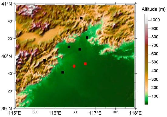
Figure 2.
Location of weather radar and the vicinity topography. The diamond denotes the CINRAD/SA radar. The squares denote the X-band radar. The radar stations marked in red are also equipped with wind lidars, while those labelled in black are not.
Secondly, we tried to use some of the observing equipment to obtain the wind field. Comparison of radar-based Doppler velocities with the wind field is one of the most important basic means of determining the type of echo. However, there are problems in obtaining true wind field velocities. Usually, the most direct way to measure the wind field is to use radiosonde. The World Meteorological Organization (WMO) requires radiosonde to be launched at the same time all over the world (within one hour before 00:00 and 12:00 UTC). Thus, in China, radiosonde is launched every day at 7:15 and 19:15 local time. However, these timings of radiosonde observations cannot include the night-time strong clear-air echoes in summer. Therefore, it is not possible to use the wind field information from the radiosonde data.
Doppler wind lidar (DWL) uses the optical Doppler effect to measure atmospheric wind speed with high spatial–temporal resolution and a long detection range and has been widely applied in scientific research and engineering applications. In addition, since lasers do not have the electromagnetic wave’s ability to penetrate and bypass, if the measurement process is affected by large particles (both biological and precipitation), it will directly produce a missing measurement rather than an erroneous value. The wind measurement products of Doppler wind lidar (Windcube 100s, Leosphere, Saclay, France) have a spatial resolution of 25 m with a temporal resolution of 20 s. Therefore, using Doppler wind lidar instead of radiosonde is a reliable way to measure wind field information in the real atmosphere.
Thirdly, in order to confirm the actual weather conditions, both the Himawari-8 satellite observations and the ERA5 reanalysis products were utilized. The Himawari-8 satellites are operated by Himawari Operation Enterprise Corporation (HOPE, Tokyo, Japen), which was established under the Japan Meteorological Agency (JMA) Private Finance Initiative project. Observation data are transmitted through HOPE to JMA, which processes the information and disseminates products to users. The Himawari-8 satellite has facilitated the undertaking of a multitude of research projects, yielding a substantial corpus of findings.
ERA5 has been the fifth generation ECMWF reanalysis for the global climate and weather for the past 8 decades. Data are available from 1940 onwards. ERA5 replaces the ERA-Interim reanalysis. Reanalysis combines model data with observations from across the world into a globally complete and consistent dataset using the laws of physics. ERA5 is a state-of-the-art reanalysis product with extensive temporal coverage, high spatial and temporal resolution, and a wide range of applications in weather analysis.
The operations of all of these meteorological observation devices (except Himawari-8) are under the supervision of the China Meteorological Administration (CMA). The weather radar is also calibrated weekly and monthly according to the technical regulations of the CMA, which includes system internal calibration, receiving link calibration, rotary joint calibration, and others. Although CINRAD data have been widely used internationally and have produced a series of research results [32,33,34,35], a small number of scholars are still uncertain about the reliability of the device. Therefore, the rationality of CINRAD data is briefly analyzed for a precipitation process.
A precipitation process was selected on 15 May to demonstrate the reliability of radar data. As the process falls within the middle period of our clear-air echo research sample set, it can be considered to represent the data accuracy during the research period. Moreover, the precipitation intensity is relatively low, comparable to light rain, which allows for the straightforward analysis of radar polarization distribution characteristics during this precipitation process. In Figure 3, both the precipitation and non-precipitation echoes observed by Beijing CINRAD/SA radar are shown, and there are clear differences in the dual-polarization products between the precipitation and non-precipitation echoes. The correlation coefficient shows a clear delineation between precipitation and non-precipitation signals, with the precipitation echo having a much higher value. Similarly, differential phase and differential reflectivity also clearly identify the characteristics of precipitation and non-precipitation signals.
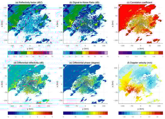
Figure 3.
Radar products from the CINRAD/SA radar, on 15 May 2021, at 14:30 UTC for an elevation angle of 1.45°.
Due to the weak reflectivity factor of the non-precipitation echoes, histograms are generated using the dual-polarization products for echoes with reflectivity factors greater than 20 dBZ, as shown in Figure 4. As expected, the correlation coefficient is approximately 0.98 for precipitation signals. The histogram of differential reflectivity shows characteristic weather values near 1 dB. The differential phase values are close to the calibration standard of 45°, and the specific differential phase is mainly between 0 and 0.1. Overall, the histograms of the radar products are consistent with the precipitation echo characteristics, demonstrating that the radar data are valid and reliable.
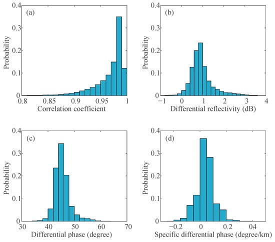
Figure 4.
Histogram of dual-polarization products with a reflectivity factor greater than 20 dBZ from the CINRAD/SA radar on 15 May 2021 at 14:30 UTC for an elevation angle of 1.45°. The histograms (a–d) represent the probability distributions of different values of radar products during precipitation, respectively.
4. Results
Clear-air echoes are frequently and typically detected from sunset, when they first appear on the radar display, until sunrise, when they gradually become less distinct. Usually, clear-air echoes are seen as shown in Figure 5. Although the reflectivity factor in Figure 5 reaches 20 dBZ, the correlation coefficient and differential reflectivity indicate non-precipitation. Hundreds of automatic weather stations owned by the Beijing Meteorological Observation Center also did not observe precipitation at this time. To prevent misinterpretation of the weather echo as a clear-air echo, which could result in unreliable outcomes, we utilized the total precipitation data from the ERA5 reanalysis product and the 11.2 μm brightness temperature from the Himawari-8 satellite to substantiate the case as a clear-air echo. Figure 6 illustrates that there were no thick clouds and no precipitation at that time. The evidence presented collectively indicates the existence of clear-air echoes in Figure 5.
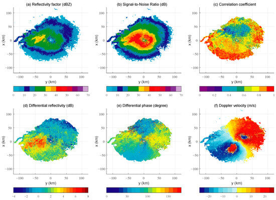
Figure 5.
Radar products from the CINRAD/SA radar, on 7 May 2021, at 15:00 UTC for an elevation angle of 1.45°.
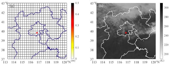
Figure 6.
Total precipitation of ERA5 reanalysis product (a) and brightness temperature of band-14 (11.2 μm) observed by Himawari-8 satellite (b), on 7 May 2021, at 15:00 UTC. The red dot represents the location of the CINRAD/SA weather radar.
In the theory of Bragg scattering, as in Equation (4), a 10 to 20 dBZ reflectivity factor needs to be greater than . However, this is far above the observed . Prior to the introduction of troposcatter, existing theories could not sufficiently explain clear-air echoes. Some researchers believe that bio-scatterers are the main cause of clear-air echoes, but there are increasing irrationalities in daily monitoring and ecological studies. Therefore, it is necessary to expose the irrationality of the original viewpoint and then to establish a correct understanding of clear-air echoes.
4.1. Paradox of Biology and Clear-Air Echo
Meteorological clear-air echoes are often confused with other types of echoes. For example, there is a common misconception that the echoes in Figure 5 are caused by the super-refraction of radar waves. It is known that super-refraction increases ground clutter at the lowest elevation and is the cause of what is normally referred to as anomalous propagation or AP echoes. In reality, the echo of super-refraction is one kind of ground clutter generated under special atmospheric conditions. The majority of clear-air echoes have significant Doppler radial velocities, which are not characteristic of ground clutter.
For a long time, the study of meteorological clear-air echoes has been based on an incomplete understanding of echoes and on the results of echo statistics. Clear-air echoes are inconsistently related to the activity of living things, but few studies have focused on this problem. Teng et al. found that the progression and movement of clear-air echoes do not conform to the rules of biological activities. The frequency distribution of dual-wavelength ratio peaks is 21.5 dB, which is in accordance with Villars–Weisskopf’s turbulence theory [36]. In this study, from 1 May to 20 May, the 58% dual-wavelength ratio between the S-band and the X-band was distributed between 18 dB and 24 dB. These results show that more than half of the clear-air echoes of CINRAD/SA at night were caused by turbulence in Beijing. However, some researchers still assume that the low correlation coefficient values and azimuthal dependencies of differential reflectivity and differential phase point to reflections from birds. However, when the carrier signal of communication passes through the wireless channel, it will also generate carrier phase deviation due to the multipath effect, propagation path bending, and other reasons.
In fact, the differential phase shift is a cumulative quantity. The differential phase is written as
where is a backscatter differential phase shift, and is the derivative of the differential phase shift, which is commonly used to estimate rain attenuation.
Zrnic and Ryzhkov state that the estimates of the backscatter differential phase are quite noisy for insects and meteorological scatterers for which is usually larger than 0.8. Further, the variation in the differential phase shift of the echoes for meteorological scatterers is small [3]. Stepanian and Horton stated that biological scatterers can have potentially large and highly variable values, which, combined with the continuous cyclic nature of the phase, results in erratic discontinuities in azimuthal functions of [37]. Stepanian et al. also stated that the texture shows a clear delineation between biological and non-biological signals, with weather having much less phase variation along the radial [38]. Thus, if clear-air echoes are produced by birds or insects, the value of changes drastically and the gradient of the (or texture) value is large and discrete.
In Figure 7, only a few areas have large values, and most echoes are devoid of bio-particle scattering. There are usually larger values of close to the radar region. This means that the of the radar wave is being altered by some scatterers close to the radar, and these alterations are then inherited by the other echoes in the radial direction. The correlation coefficients also lead to a similar conclusion. In Figure 5, there are many echoes with values of the correlation coefficient greater than 0.8 that are closer to meteorological scatterers. In addition, instantaneous vortex visualization in some studies intuitively shows that turbulence also has a directionality [39,40]. Thus, based on modern turbulence theory, it is impossible for the azimuthal correlation between and to prove bio-particle scattering.
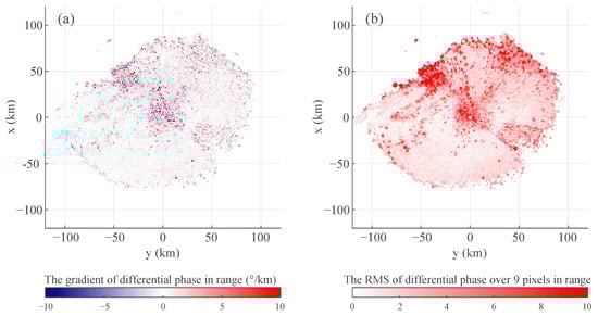
Figure 7.
The gradient of in range (a) and the root-mean-square (RMS) deviation of over 9 pixels in range (b), on 7 May 2021, at 15:00 UTC for an elevation angle of 1.45°.
It is easy to see that some of the existing studies based on isotropic turbulence have significant shortcomings. Some researchers have miscalculated the complexity of the turbulence. This leads to an excessive number of bio-echo samples, resulting in many statistical results that include a significant amount of clear-air turbulence scattering. Therefore, we briefly reiterate the abiotic nature of the echoes based on the differences between the Doppler velocity and the wind field.
4.1.1. Velocity Analysis
The clear-air echoes in Figure 5 are similar to the echoes caused by the migration of many different species of scattering birds [41]. It is unlikely that these echoes are caused by insects, as an insect has a higher differential reflectivity and a relatively lower differential phase. It is also unlikely that these echoes are caused by birds because of the velocity–azimuth display (VAD).
VAD analysis is used to determine spatially averaged kinematic properties of the velocity field. The VAD of the wind field resembles a sine function of the radar azimuth angle. The large differences in the observed radial velocity are usually regarded as the result of the creatures’ own flight speeds during bird migration. Figure 7 shows a velocity field close to a sine function, which was the same passage of a cold front as observed using an operational weather radar at De Bilt [42]. Only a small part of the residual error near and to the west of the radar shows signs of bird activity in Figure 8. And most of the echoes show no sign of biological activity.
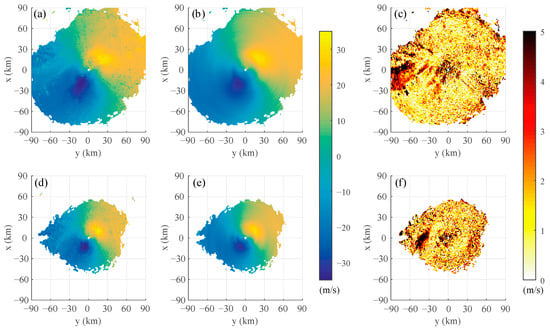
Figure 8.
Doppler velocity fields (a,d) and fields fitted by sinusoidal function (b,e), on 7 May 2021, at 15:00 UTC. Panels (c,f) show the difference between the velocity field and the field of sinusoidal fitting. The elevation angles of (a–c) and (d–f) are 1.5° and 2.4°, respectively.
To prove our point, we used two wind lidars (Windcube 100S) to check the wind field differences between the wind lidars (WLSs) and the weather radar (CINRAD). One wind lidar is located at the same site as the weather radar, as shown by the red dots in Figure 9a,b. The location of the other lidar is shown by the blue dot in Figure 9a,b. Reanalysis data from the European Centre for Medium-Range Weather Forecasts (ECMWF) showed that the wind field was uniform at that time.
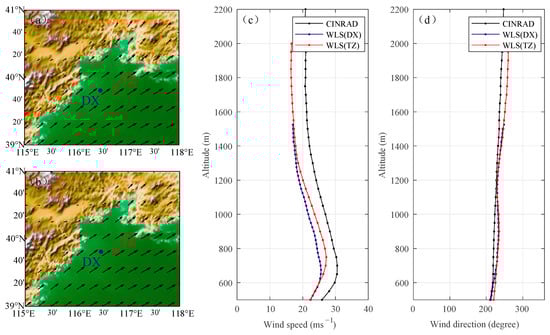
Figure 9.
(a,b) are locations of the WLSs and CINRAD. (c,d) are profiles of mean wind speed and wind direction from 13:30 to 15:30 UTC on 7 May 2021. The WLSs are located separately in the DX and TZ stations. CINRAD is also located in the DX station. In (a,b), the arrow represents the wind field of the ECMWF reanalysis data at a height of 900 hPa at 14:00 (a) and 15:00 (b).
Since the radial velocity field of the radar behaves as a sine function in Figure 9, we can substantially simplify the computation of the velocity, based on the meaning of radial velocity. The sine function at any range represents the radar radial component of the velocity field at that altitude, which means the extreme value of the sine function is the velocity and the direction in which the extreme value is located is the direction of motion. Notably, as the wind lidar is a device of vertical observation, the accuracy of comparison between weather radar and lidar will decrease with increasing distance between them. Therefore, the range of valid data is limited to 50 km in the calculation of weather radar wind profiles empirically.
It is clear that if the movement of the CINRAD echo is similar to the wind field observed with the lidar, then most of the clear-air echoes are not generated by bird activity because there is no corresponding speed of bird movement. In Figure 9c there are no significant differences except for a top-down systematic deviation of less than 5 m/s, which is too small for bird flight speeds as migrating birds fly at air speeds slightly above 10 m/s [43].
However, the flight of birds may also contaminate the laser wind radar observations. We therefore show the laser wind radar results for a longer period of time. Due to the nature of lasers, they cannot bypass bird bodies, and bird activity will directly block the laser beam. Therefore, we focus on the carrier-to-noise ratio (CNR) of the laser wind radar and the effective detection height of the laser radar in Figure 10 and Figure 11.
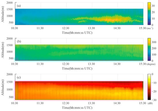
Figure 10.
Horizontal wind profiles measured with the WLS (Windcube 100s) at DX station on 7 May 2021. Panel (a) is the horizontal wind speed (m/s), and panel (b) is the horizontal wind direction (degrees). Panel (c) is the carrier-to-noise ratio (CNR in dB) of the WLS.
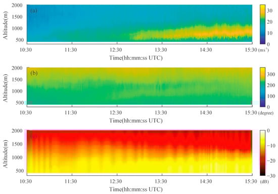
Figure 11.
Same as Figure 10 but for WLS at TZ station.
In Figure 10c and Figure 11c, the CNRs of two lidars do not change with the enhancement of the clear-air echo, which is shown in Figure 11c. Neither lidar observes a decrease in laser detection height. There are no organisms blocking the laser’s path through the atmosphere. The data from the lidars are therefore reliable. More importantly, this shows that the clear-air echoes from the weather radar move strictly according to the rules of the wind, as shown in Figure 12. The changes in the wind field observed with the lidars coincide with changes in the clear-air echo motion, as shown in Figure 10, Figure 11 and Figure 12. Therefore, the view that the echo is generated by bird activity is inaccurate.
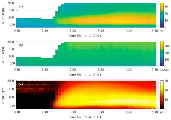
Figure 12.
Panels (a,b) are the mean horizontal wind speed (m/s) and the mean horizontal wind direction (degrees) computed by the S-band weather radar of the DX station on 7 May 2021. Panel (c) is the time–height cross section of the radar reflectivity factor at the same time.
4.1.2. Distribution Analysis
In fact, not only does velocity show the abiotic character of the clear-air echoes, but the plan position indicator also provides an intuitive representation of the contradiction between the echoes and the characteristics of biological activity. Figure 13 shows a continuous change in the plan position indicator of the reflectivity factor and clearly shows that the echoes have changed with the radar station as the center, but not the ‘habitat’. Furthermore, the geometry and distribution of the echoes are essentially unchanged, but these echoes have a high Doppler velocity in Figure 14. In addition, the clear-air echoes persist over the two international airports. Such a high level of bird activity would be extremely dangerous for flights and airports.
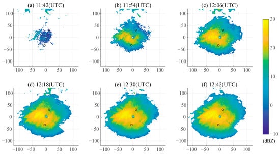
Figure 13.
Composite reflectivity for 2 h from CINRAD/SA, 7 May 2021. (a–f) Continuous observations from CINRAD/SA at 12 min intervals from 11:42 to 12:42. The horizontal and vertical coordinates are the distances (km) in west–east and south–north directions, respectively. The black circles on the map indicate the locations of Beijing Capital International Airport and Beijing Daxing International Airport.
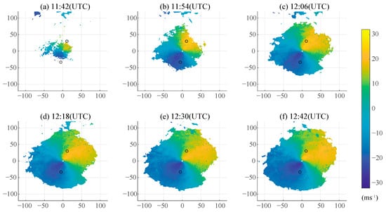
Figure 14.
Mean Doppler velocity for 2 h from CINRAD/SA, 7 May 2021. (a–f) Continuous observations from CINRAD/SA at 12 min intervals from 11:42 to 12:42. The horizontal and vertical coordinates are the distances (km) in west–east and south–north directions, respectively. The black circles on the map indicate the locations of Beijing Capital International Airport and Beijing Daxing International Airport.
To confirm the movement of the clear-air echoes, the range–height cross section of the reflectivity factor in the azimuth of the wind direction is shown in Figure 15. As shown in Figure 15, the clear-air echo signal is enhanced along the height at all times, but does not vary with range and time. Even assuming that there is a radar cross-section (RCS) difference between the head and tail of the bird, this does not explain the lack of movement of the clear-air echo on the same side of the radar. If the speed of the scatterers is estimated to be 30 m/s, then the scatterers were flying at least 20 km every 12 min (between each subplot of Figure 15). However, Figure 15 shows no matching motion. This means that the scatterers are not moving but are constantly repeating the cycle of generation and extinction in the atmosphere.
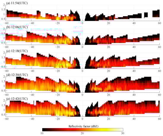
Figure 15.
Range–height cross section of Z following the azimuthal direction (azimuth: 222°). (a–e) Continuous observations from CINRAD/SA at 6 min intervals from 11:54 to 12:42, 7 May 2021. The horizontal axis is the distance (km) along the wind direction and the vertical axis is the height (km).
4.1.3. Dual-Wavelength Analysis
Some researchers have also suggested that Rayleigh scattering from bugs and dust can cause the echo of active radar in the atmosphere. It is possible that the troposcatter models presented, which include empirically derived constants, presumably combine both effects. Therefore, we also need to rule out this negative possibility.
It is known that the scattering intensity of Rayleigh scattering is inversely proportional to the fourth power of the wavelength. This means that X-band radar would be considerably more sensitive to Rayleigh scattering and less sensitive to troposcatter. Figure 16 shows the composite reflectivity from the Beijing X-band weather radar network at the same time as in Figure 2. We can see that the difference in reflectivity factor between the S-band and the X-band is inconsistent with Rayleigh scattering. The value of the composite reflectivity in the X-band is much smaller than that in the S-band.
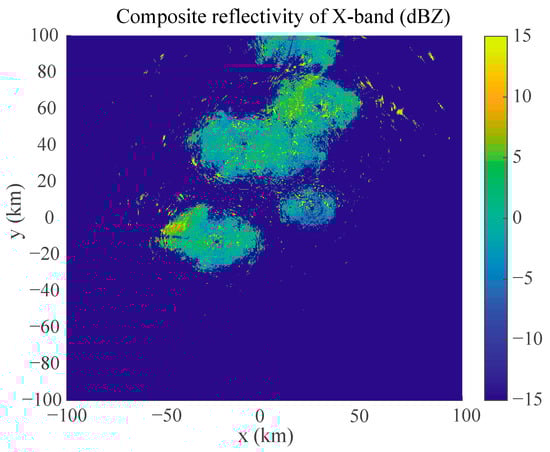
Figure 16.
Composite reflectivity from the Beijing X-band weather radar network at same time as in Figure 5.
The value of composite reflectivity in the X-band is considerably smaller than that in the S-band for two principal reasons. In the case of tropospheric scattering, as illustrated in Equations (4) and (5), the radar cross-section and reflectivity factor are both power functions of wavelength. Consequently, the observations exhibit notable inconsistencies when examined across different wavelengths. Moreover, as the minimum scale of turbulence increases with height, the turbulence observable in the X-band will disappear at an earlier height than in the S-band. Consequently, the area and intensity of the X-band echo will also be considerably reduced in comparison to that of the S-band.
We also chose the closest X-band radar to CINRAD/SA (about 30 km away) so that we could obtain the results of RHI within the same space. The RHI (Figure 17) shows many variations, both in the intensity of the echoes and in the vertical distribution of the echoes. However, we cannot identify the sensitive single of Rayleigh scattering in Figure 17. The reflectivity factor of the X-band is also much smaller than that of the S-band.
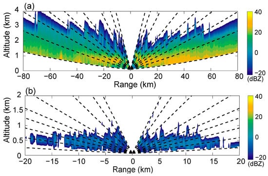
Figure 17.
Range–height cross-sections of reflectivity factor in S-band (a) and X-band (b). The black dashed lines in (a,b) represent the radar beams of VCP21. The positive direction of cross-sections in (a,b) is on the azimuth of 78° (a) and the azimuth of 282° (b), respectively, which means that (a,b) are facing each other.
4.2. Transmission Loss Comparisons
In Equation (25), a relationship was established between the transmission loss of radar and troposcatter via the derivation and ITU-R recommendations. The clear-air echo signal caused by troposcatter should follow the ITU-R propagation model. Detailed guidance on the prediction of transmission loss can be found in ITU-R P.617 and P.2001, which were introduced in Section 2.3.2. To demonstrate the substantial role of troposcatter in radar observations, the transmission loss obtained via radar and the ITU-R recommendations are compared in Figure 18.
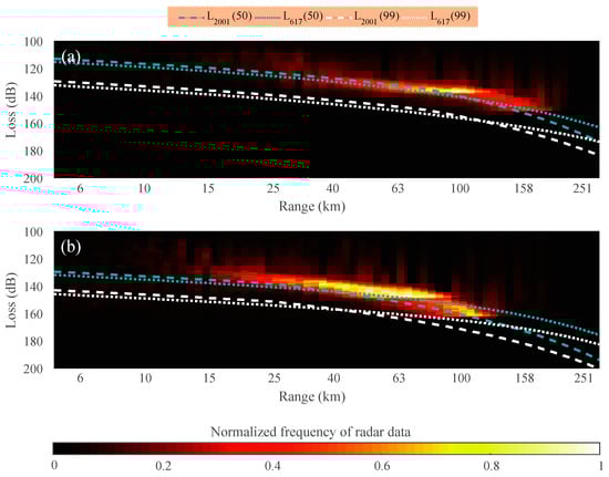
Figure 18.
Radar transmission loss with range for elevation angles of 0.5° (a) and 1.45° (b) every day from 12:30 to 16:00 UTC in May. The transmission loss predictions of ITU-R are the lines in each subgraph.
In Figure 18, different ITU-R standards are represented by different line types, and line colors indicate various non-exceedance percentages. The radar transmission loss is colored to reflect its frequency distribution from 12:30 to 16:00 UTC everyday throughout May. The results show that the radar transmission loss aligns with ITU-R recommendations, with ITU-R P.2001 being more consistent with radar transmission loss than ITU-R P.617. As the distance increases, the transmission loss of the radar also increases, and the rate of increase gradually accelerates, which is consistent with the transmission loss variation characteristics of ITU-R recommendations.
Although the scattering coefficient is an estimated value, resulting in a potential error, the radar transmission loss is still primarily distributed near the ideal loss recommended by the ITU. Therefore, the actual non-exceedance percentage corresponding to radar is undetermined. Overall, the radar transmission loss is consistent with ITU-R’s transmission loss for troposcatter, which proves the role of troposcatter in clear-air radar echoing. Moreover, there should be a linear regression relationship between the transmission loss (in dB) and height.
In general, the dielectric constant tends to be exponentially distributed. As shown in Equation (5), the variation in the scattering cross-section for troposcatter with height is the same as the variation in the dielectric constant. It makes the transmission loss also exponentially distributed like the dielectric constant. In Figure 19 we found that the transmission loss (in dB) has a linear relationship with height. Therefore, we deem that most clear-air echoes are caused by tropospheric scattering due to turbulence because the S-band weather radar transmission loss of clear-air echoes is consistent with the value of tropospheric scattering. The theory of tropospheric scattering is a supplement to the theory of Bragg scattering. Based on the theory of tropospheric scattering, we can explain the problem of the excessive signal strength of clear-air echoes. The original misunderstanding was caused by neglecting the impact of incoherent reflection by irregular layers.
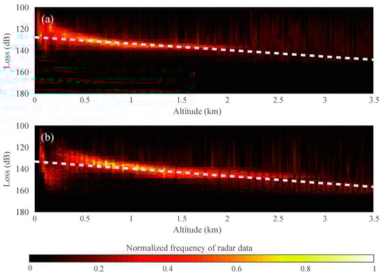
Figure 19.
Radar transmission loss with altitude for elevation angles of 0.5° (a) and 1.45° (b) every day from 12:30 to 16:00 UTC in May. The white dotted line is the regression line.
Notably, in Figure 19, there is a disorder in the loss below the height of 500 m. This may be caused by biological scattering. The feature of biological scattering can also be found in the echoes close to the radar (i.e., the heights of the echo are low) in Figure 7 and Figure 8. In these two figures, the echoes close to the radar have different characteristics from the other echoes, such as more discrete velocities and values, which are characteristic of biological activity. Therefore, biological scattering is still one of the causes of the clear-air echoes below 500 m.
5. Discussion
5.1. Biological Applications
In Section 4, we proposed that Bragg scattering is a special case of tropospheric scattering. This means that clear-air echoes caused by atmospheric factors are consistent with the ITU-R’s recommendations. As the ITU-R recommended, the relationship between the reflectivity factor of weather radar and the observation range has been clarified by the equivalent transmission loss, Equation (25). However, we can see that some echoes did not meet the ITU-R recommendations in Figure 19. We assume those echoes were generated by particle scattering (especially biological). Therefore, we plotted the echoes that did not meet the ITU-R recommendations, as shown in Figure 20. In Figure 20, we extracted those echoes for which the radar transmission loss was 3 dB larger than the ITU-R recommendations. For reliability, echoes with an SNR less than 12 dB were discarded. It can be seen that the distribution of the radar transmission loss (Figure 20a) is relatively close to the theoretical value (Figure 20b). Some of the echoes with large differences have large values of differential reflectivity (Figure 20c). There are also parts of the ring-like echoes suggesting that the organisms were congregating, which may be due to the stratification of insect migration.
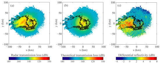
Figure 20.
Radar transmission loss (a) and theoretical values based on the ITU-R model (b), on 7 May 2021, at 15:00 UTC for an elevation angle of 1.45°. The figure also shows the differential reflectivity (c). The area surrounded by the black outline is the suspected area of biological activity.
These features seem to indicate that these echoes were caused by biological activity. However, no similar biological echoes were observed in the X-band (in Figure 16). There are two completely different interpretations for this phenomenon. One is that the creatures happen to be in the blind spot of the X-band. The other is that the mountains unexpectedly make the tropospheric scattering stronger. Although we recognize the role of terrain, it is difficult to completely deny the role of organisms in echo generation. Thus, we need longer and more sophisticated observations to solve this problem.
5.2. Calibration Coefficient
In the equation of radar transmission loss, we established a calibration coefficient to balance the intensities between backscattering and the grazing angle direction. However, the precise setting of this coefficient is not possible. We observed that this correction resulted in an increase in error as the grazing angle (which is related to scattering angles) increased. Although we believe that the scattering coefficient setting is somewhat excessive, we have no other reasonable assumption except to refer to the coefficient of Fresnel reflection in the absence of a clear physical model. Furthermore, it is necessary to correct for the application of the ITU-R recommendations to radar. As the radar elevation increases, the angular dependent loss in the ITU-R recommendations increases due to the decrease in the transceiver shared scattering volume. However, the radar transceiver shared volume remains constant. Therefore, as the elevation angle increases, the transmission loss of the ITU-R recommendations rapidly increases. Although the change in radar transmission loss is limited, the trend of the two changes with distance is similar. Therefore, we can see in Figure 18 that the radar transmission loss at an elevation of 1.45° is farther from the ITU-R recommendation than the radar transmission loss at an elevation of 0.5°. As the elevation angle of the radar increases, this difference becomes more apparent. Thus, when applying the recommendations of the ITU-R, it is necessary to consider the overestimation caused by volume loss at the large radar elevation.
5.3. Scattering Model
The most crucial issue is the scattering model for troposcatter. Troposcatter is a combination of three models: turbulence scattering, stable layer reflection, and irregular layer reflection. Turbulence scattering and stable layer reflection have corresponding atmospheric models. However, the model of irregular layer reflection is not yet clear, and we can only provide some conjectures. The theory of irregular layer reflection suggests that these irregular layers, with a large refractive index gradient, are formed by the intersection of cooling and heating air masses. Moreover, strong convection often leads to precipitation. Recently, it has been proposed that large values of reflectivity correspond to large Richardson numbers and small amounts of turbulent mixing [36]. This means that clear-air echoes are affected by strong turbulent mixing and require unmixed air masses to maintain inhomogeneity. Thus, the wildly fluctuating gradient of the refractive index in the source model is more likely caused by the non-uniformity of meteorological elements rather than air convection. Some meteorologists have privately communicated that weather radars located on ships at sea rarely observe clear-air echoes. We consider that the uniform underlying surface of the ocean greatly reduces the non-uniformity of meteorological elements, thereby weakening the intensity of clear-air echoes.
The recommendations of the ITU-R give various transmission loss parameters for different climatic regions. This map shows that meteorological conditions play an important role in troposcatter. However, the impact of meteorology on tropospheric scattering is too complex to be captured by a single model. For wireless communication, it is crucial to have a thorough understanding of the weather patterns in a specific region before implementing a tropospheric scatter communication system. The use of advanced modeling techniques, such as numerical weather prediction models, can provide more accurate predictions of transmission loss and improve the reliability of communication systems. Continued research and the improvement of tropospheric scatter technology will enable the development of more robust and effective communication systems. For atmospheric science, understanding troposcatter and its models is important for a variety of fields, including meteorology, environmental science, and astronomy. By studying troposcatter, we can gain a better understanding of the properties of the Earth’s atmosphere, the way that air mass affects reflection and transmission through the troposphere, and the impact of atmospheric microscale inhomogeneity on weather.
In this manuscript, we have presented an introduction that explores and confirms the occurrence of tropospheric scattering in the atmosphere. Although numerous issues remain unresolved, it is crucial to acknowledge that these tasks cannot be accomplished overnight. We hope this manuscript can offer a new research direction and enhance awareness among researchers.
5.4. Boundary Layer Structure
In the first section, we stated that the value varies in the range −2 dB to 2 dB, and that is exactly what happens in reality. However, the values of turbulent air have also been considered to be close to 0 dB in several studies [27,44,45]. This may seem contradictory, but this is not the case. Notably, the 0 dB echo is often observed in the entrainment layer, which is located at the top of the boundary layer. Due to the effects of penetrative convection and entrainment, thermals reciprocate in the layer [46]. Therefore, we suggest that the reciprocation brings the atmosphere closer to a locally homogeneous isotropic state. This means that clear-air echoes can be used to study the state of the microscale atmospheric motion. We also found that, in some cases, radars in economically developed and populous areas like Beijing and Tianjin observe stronger clear-air echoes than these detected by radars in the countryside. This may be because, in a large city, there are more inhomogeneous air masses caused by human activities and urban architecture. Clear-air echoes can also be used to assess the effects of urban underlying surfaces in the boundary layer. Related studies will be conducted in the future.
6. Conclusions
In this study, weather radar was considered as a special wireless communication device. Via the derivation of the radar range equation, the transmission loss of radar clear-air echoes was calculated in order to establish a relationship with the troposcatter. The results indicate that the radar transmission loss is in accordance with ITU-R recommendations, with ITU-R P.2001 demonstrating greater consistency with radar loss than ITU-R P.617. Additionally, a linear regression relationship exists between the transmission loss (in dB) and the altitude. The result of the study shows that most clear-air echoes are caused by tropospheric scattering due to turbulence. The scattering of clear-air echoes is consistent with troposcatter theory. The theory of tropospheric scattering is complementary to the theory of Bragg scattering. Tropospheric scattering can be thought of as general Bragg scattering.
We also found that some echoes do not comply with the recommendations of the ITU-R and are more likely to be caused by biological activity. This provides a new approach by which to recognize biological echoes.
The connection between wireless communication and atmospheric science has been established using the theory of troposcatter. However, there are still many issues that need to be addressed. The geometrical structure of the troposcatter, especially incoherent reflection by irregular layers, remains obscure. The scattering characteristics of microscale air mass (centimeter level) under the influence of meteorological background effects poses great challenges. This may be an opportunity for exploring the microscale atmospheric structure. A more objective and comprehensive study of troposcatter echoes can effectively promote the progress of atmospheric physics.
Author Contributions
Conceptualization, Y.T. and S.M.; methodology, Y.T.; software, Y.T.; validation, Y.T.; formal analysis, Y.T.; investigation, Y.T.; resources, S.M. and H.C.; data curation, L.W., Y.X. and S.L.; writing—original draft preparation, Y.T. and T.L.; writing—review and editing, Y.T. and T.L.; visualization, Y.T. and T.L.; supervision, S.M., H.C. and L.W.; project administration, Y.T., S.M. and H.C.; funding acquisition, Y.T., S.M. and H.C. All authors have read and agreed to the published version of the manuscript.
Funding
This research was funded by the National Natural Science Foundation of China, grant number 42205145.
Data Availability Statement
Data available on request due to legal.
Conflicts of Interest
The authors declare no conflicts of interest. The funders had no role in the design of this study; in the collection, analyses, or interpretation of data; in the writing of the manuscript; or in the decision to publish the results.
References
- Kusunoki, K. A Preliminary Survey of Clear-Air Echo Appearances over the Kanto Plain in Japan from July to December 1997. J. Atmos. Ocean. Technol. 2002, 19, 1063–1072. [Google Scholar] [CrossRef]
- Wilson, J.W.; Weckwerth, T.M.; Vivekanandan, J.; Wakimoto, R.M.; Russell, R.W. Boundary Layer Clear-Air Radar Echoes: Origin of Echoes and Accuracy of Derived Winds. J. Atmos. Ocean. Technol. 1994, 11, 1184–1206. [Google Scholar] [CrossRef]
- Zrnic, D.; Ryzhkov, A. Observations of insects and birds with a polarimetric radar. IEEE Trans. Geosci. Remote Sens. 1998, 36, 661–668. [Google Scholar] [CrossRef]
- Birnir, B. The Kolmogorov–Obukhov Statistical Theory of Turbulence. J. Nonlinear Sci. 2013, 23, 657–688. [Google Scholar] [CrossRef]
- Batchelor, G.K.; Townsend, A.A. The nature of turbulent motion at large wave-numbers. Proc. R. Soc. London Ser. A. Math. Phys. Sci. 1949, 199, 238–255. [Google Scholar] [CrossRef]
- Siggia, E.D. Numerical study of small-scale intermittency in three-dimensional turbulence. J. Fluid Mech. 1981, 107, 375–406. [Google Scholar] [CrossRef]
- Korotkova, O.; Toselli, I. Non-Classic Atmospheric Optical Turbulence: Review. Appl. Sci. 2021, 11, 8487. [Google Scholar] [CrossRef]
- Andrews, L.C.; Toselli, I.; Phillips, R.L.; Ferrero, V. Free-space optical system performance for laser beam propagation through non-Kolmogorov turbulence. Opt. Eng. 2008, 47, 026003. [Google Scholar] [CrossRef]
- Wang, F.; Toselli, I.; Li, J.; Korotkova, O. Measuring anisotropy ellipse of atmospheric turbulence by intensity correlations of laser light. Opt. Lett. 2017, 42, 1129–1132. [Google Scholar] [CrossRef]
- Beason, M.; Smith, C.; Coffaro, J.; Belichki, S.; Spychalsky, J.; Titus, F.; Crabbs, R.; Andrews, L.; Phillips, R. Near ground measure and theoretical model of plane wave covariance of intensity in anisotropic turbulence. Opt. Lett. 2018, 43, 2607–2610. [Google Scholar] [CrossRef]
- Ottersten, H. Atmospheric Structure and Radar Backscattering in Clear Air. Radio Sci. 1969, 4, 1179–1193. [Google Scholar] [CrossRef]
- Ottersten, H.; Hardy, K.R.; Little, C.G. Radar and sodar probing of waves and turbulence in statically stable clear-air layers. Bound.-Layer Meteorol. 1973, 4, 47–89. [Google Scholar] [CrossRef]
- Li, L.; Wu, Z.-S.; Lin, L.-K.; Zhang, R.; Zhao, Z.-W. Study on the Prediction of Troposcatter Transmission Loss. IEEE Trans. Antennas Propag. 2016, 64, 1071–1079. [Google Scholar] [CrossRef]
- Zhang, M.G. Tropospheric Scatter Propagation; Publishing House of Electronics Industry: Beijing, China, 2004. [Google Scholar]
- Booker, H.; Gordon, W. A Theory of Radio Scattering in the Troposphere. Proc. IRE 1950, 38, 401–412. [Google Scholar] [CrossRef]
- Bullington, K. Reflections from an Exponential Atmosphere. Bell Syst. Tech. J. 1963, 42, 2849–2867. [Google Scholar] [CrossRef]
- Friis, H.T.; Crawford, A.B.; Hogg, D.C. A Reflection Theory for Propagation Beyond the Horizon *. Bell Syst. Tech. J. 1957, 36, 627–644. [Google Scholar] [CrossRef]
- Mueller, E.A.; Larkin, R.P. Insects Observed Using Dual-Polarization Radar. J. Atmos. Ocean. Technol. 1985, 2, 49–54. [Google Scholar] [CrossRef]
- Gossard, E.E. Radar Research on the Atmospheric Boundary Layer; David, A., Ed.; Radar in Meteorology: Battan Memorial and 40th Anniversary Radar Meteorology Conference; American Meteorological Society: Boston, MA, USA, 1990. [Google Scholar]
- Martin, W.J.; Shapiro, A. Discrimination of Bird and Insect Radar Echoes in Clear Air Using High-Resolution Radars. J. Atmos. Ocean. Technol. 2007, 24, 1215–1230. [Google Scholar] [CrossRef]
- Kolmogorov, A.N.; Levin, V.; Julian, C.R.H.; Owen, M.P.; David, W. The local structure of turbulence in incompressible viscous fluid for very large Reynolds numbers. Proceedings of the Royal Society of London. Ser. A Math. Phys. Sci. 1997, 434, 9–13. [Google Scholar]
- Kolmogorov, A.N. A refinement of previous hypotheses concerning the local structure of turbulence in a viscous in-compressible fluid at high Reynolds number. J. Fluid Mech. 2006, 13, 82–85. [Google Scholar] [CrossRef]
- Doviak, R.J.; Dušan, S.Z. Doppler Radar and Weather Observations, 2nd ed.; Richard, J.D., Dušan, S.Z., Eds.; Academic Press: San Diego, CA, USA, 2006. [Google Scholar]
- Knight, C.A.; Miller, L.J. First Radar Echoes from Cumulus Clouds. Bull. Am. Meteorol. Soc. 1993, 74, 179–188. [Google Scholar] [CrossRef]
- Hardy, K.R.; Katz, I. Probing the clear atmosphere with high power, high resolution radars. Proc. IEEE 1969, 57, 468–480. [Google Scholar] [CrossRef]
- Cowley, J.M. Diffraction Physics, 3rd ed.; Cowley, J.M., Ed.; North-Holland: Amsterdam, The Netherlands, 1995. [Google Scholar]
- Richardson, L.M.; Cunningham, J.G.; Zittel, W.D.; Lee, R.R.; Ice, R.L.; Melnikov, V.M.; Hoban, N.P.; Gebauer, J.G. Bragg Scatter Detection by the WSR-88D. Part I: Algorithm Development. J. Atmos. Ocean. Technol. 2017, 34, 465–478. [Google Scholar] [CrossRef]
- Lee, I.-S.; Noh, J.-H.; Oh, S.-J. A Survey and analysis on a troposcatter propagation model based on ITU-R recommendations. ICT Express 2023, 9, 507–516. [Google Scholar] [CrossRef]
- Recommendation ITU-R P.617: Propagation Prediction Techniques and Data Required for the Design of Trans-Horizon Radio-Relay Systems. Available online: https://www.itu.int/dms_pubrec/itu-r/rec/p/R-REC-P.617-5-201908-I!!PDF-E.pdf (accessed on 30 August 2023).
- Recommendation ITU-R P.2001: A General Purpose Wide-Range Terrestrial Propagation Model in the Frequency Range 30 MHz to 50 GHz. Available online: https://www.itu.int/dms_pubrec/itu-r/rec/p/R-REC-P.2001-5-202308-I!!PDF-E.pdf (accessed on 30 August 2023).
- Chen, Y.; Zou, Q.; Han, J.; Cluckie, I. Cinrad data quality control and precipitation estimation. Proc. Inst. Civ. Eng. Water Manag. 2009, 162, 95–105. [Google Scholar] [CrossRef]
- Sheng, C.; Gao, S.; Xue, M. Short-range prediction of a heavy precipitation event by assimilating Chinese CINRAD-SA radar reflectivity data using complex cloud analysis. Meteorol. Atmos. Phys. 2006, 94, 167–183. [Google Scholar] [CrossRef]
- Chu, Z.; Yin, Y.; Gu, S. Characteristics of velocity ambiguity for CINRAD-SA Doppler weather radars. Asia-Pac. J. Atmos. Sci. 2013, 50, 221–227. [Google Scholar] [CrossRef]
- Chao, C.; Li-ping, L.; Sheng, H.; Zhi-fang, W.; Chong, W.; Yang, Z. Operational Evaluation of the Quantitative Precipitation Estimation by a CINRAD-SA Dual Polarization Radar System. J. Trop. Meteorol. 2020, 26, 176–187. [Google Scholar] [CrossRef]
- Han, S.; Dong, X.; Chen, X.; Liu, F.; Zhu, L. Evaluating Reflectivity Quality of the New Airship-Borne Weather Radar Using the S-Band Ground-Based Weather Radar in China. In Proceedings of the IGARSS 2023—2023 IEEE International Geoscience and Remote Sensing Symposium, Pasadena, CA, USA, 16–21 July 2023; pp. 3811–3814. [Google Scholar]
- Teng, Y.; Li, T.; Ma, S.; Chen, H. Turbulence: A Significant Role in Clear-Air Echoes of CINRAD/SA at Night. Remote Sens. 2023, 15, 1781. [Google Scholar] [CrossRef]
- Stepanian, P.M.; Horton, K.G. Extracting Migrant Flight Orientation Profiles Using Polarimetric Radar. IEEE Trans. Geosci. Remote Sens. 2015, 53, 6518–6528. [Google Scholar] [CrossRef]
- Stepanian, P.M.; Horton, K.G.; Melnikov, V.M.; Zrnić, D.S.; Gauthreaux, S.A., Jr. Dual-polarization radar products for biological applications. Ecosphere 2016, 7, e01539. [Google Scholar] [CrossRef]
- Marxen, O.; Zaki, T.A. Turbulence in intermittent transitional boundary layers and in turbulence spots. J. Fluid Mech. 2018, 860, 350–383. [Google Scholar] [CrossRef]
- Vassilicos, J.C. Turbulence and intermittency. Nature 1995, 374, 408–409. [Google Scholar] [CrossRef]
- Van Den Broeke, M.S. Polarimetric Radar Observations of Biological Scatterers in Hurricanes Irene (2011) and Sandy (2012). J. Atmos. Ocean. Technol. 2013, 30, 2754–2767. [Google Scholar] [CrossRef][Green Version]
- Holleman, I.; Van Gasteren, H.; Bouten, W. Quality Assessment of Weather Radar Wind Profiles during Bird Migration. J. Atmos. Ocean. Technol. 2008, 25, 2188–2198. [Google Scholar] [CrossRef]
- Gauthreaux, S.A.; Carroll, G.B. Displays of Bird Movements on the WSR-88D: Patterns and Quantifica-tion *. Weather. Forecast. 1998, 13, 453–464. [Google Scholar] [CrossRef]
- Richardson, L.M.; Zittel, W.D.; Lee, R.R.; Melnikov, V.M.; Ice, R.L.; Cunningham, J.G. Bragg Scatter Detection by the WSR-88D. Part II: Assessment of ZDR Bias Estimation. J. Atmos. Ocean. Technol. 2017, 34, 479–493. [Google Scholar] [CrossRef]
- Banghoff, J.R.; Stensrud, D.J.; Kumjian, M.R. Convective Boundary Layer Depth Estimation from S-Band Du-al-Polarization Radar. J. Atmos. Ocean. Technol. 2018, 35, 1723–1733. [Google Scholar] [CrossRef]
- Stull, R.B. An Introduction to Boundary Layer Meteorology; China Meteorological Press: Beijing, China, 1988.


Disclaimer/Publisher’s Note: The statements, opinions and data contained in all publications are solely those of the individual author(s) and contributor(s) and not of MDPI and/or the editor(s). MDPI and/or the editor(s) disclaim responsibility for any injury to people or property resulting from any ideas, methods, instructions or products referred to in the content. |
© 2024 by the authors. Licensee MDPI, Basel, Switzerland. This article is an open access article distributed under the terms and conditions of the Creative Commons Attribution (CC BY) license (https://creativecommons.org/licenses/by/4.0/).