Hyperspectral Image Denoising by Pixel-Wise Noise Modeling and TV-Oriented Deep Image Prior

Abstract

Model-based hyperspectral image (HSI) denoising methods have attracted continuous attention in the past decades, due to their effectiveness and interpretability. In this work, we aim at advancing model-based HSI denoising, through sophisticated investigation for both the fidelity and regularization terms, or correspondingly noise and prior, by virtue of several recently developed techniques. Specifically, we formulate a novel unified probabilistic model for the HSI denoising task, within which the noise is assumed as pixel-wise non-independent and identically distributed (non-i.i.d) Gaussian predicted by a pre-trained neural network, and the prior for the HSI image is designed by incorporating the deep image prior (DIP) with total variation (TV) and spatio-spectral TV. To solve the resulted maximum a posteriori (MAP) estimation problem, we design a Monte Carlo Expectation–Maximization (MCEM) algorithm, in which the stochastic gradient Langevin dynamics (SGLD) method is used for computing the E-step, and the alternative direction method of multipliers (ADMM) is adopted for solving the optimization in the M-step. Experiments on both synthetic and real noisy HSI datasets have been conducted to verify the effectiveness of the proposed method.

1. Introduction

Hyperspectral images (HSIs) are acquired by high spectral resolution sensors, which generally have hundreds of bands ranging from ultraviolet to infrared wavelengths. Due to the richness of its spatial and spectral information, HSIs have been widely used in many applications [1,2,3,4,5], such as environmental monitoring, military surveillance and mineral exploration. However, due to various factors, including thermal electronics, dark current and stochastic error of photocounting in an imaging process, HSIs inevitably suffer from severe noise during the acquisition process, which results in inconvenience to the subsequent tasks. Therefore, as an important pre-processing step, HSI denoising has attracted much attention in the past decades.

Current HSI denoising methods can be roughly divided into two categories, i.e., model-driven methods and data-driven ones. Recently, due to the rapid advances in deep learning studies, data-driven methods, which try to directly learn a denoiser from paired noisy-clean HSIs in an end-to-end way, have attracted more attention [6,7,8,9,10]. Though they can achieve promising denoising results, the performance of these kinds of methods highly depends on the quality of training data and may not generalize well to realistic HSIs since the real noise is much more complex than that contained in the training data. Therefore, in this work, we are more interested in the model-driven HSI denoising methods, while also trying to borrow the merits of the data-driven ones.

Model-based HSI methods are generally constructed according to the following observation model:

$$\mathcal{Y}=\mathcal{X}+\mathcal{E}$$

(1)

where $\mathcal{X}\in {\mathbb{R}}^{h\times w\times b}$ denotes the clean HSI, $\mathcal{E}\in {\mathbb{R}}^{h\times w\times b}$ the noise, and $\mathcal{Y}\in {\mathbb{R}}^{h\times w\times b}$ the corresponding noisy observation. Based on (1), one can formulate the HSI denoising problem as the following optimization, in general:

$$\underset{\mathcal{X}}{\min }L(\mathcal{X},\mathcal{Y})+R(\mathcal{X}),$$

(2)

where $L(\mathcal{X},\mathcal{Y})$ is often referred to as the fidelity term, which ensures that the estimated clean HSI $\mathcal{X}$ is not too far from the noisy observation $\mathcal{X}$ and is related to the assumption of the noise $\mathcal{E}$; $R(\mathcal{X})$ is the regularization term, which characterizes the prior knowledge about the intrinsic structures underlying the clean HSI. As can be seen from (2), both the fidelity and the regularization terms contribute to the final estimation $\mathcal{X}$, and therefore, how to properly design them to better characterize the intrinsic structures of the noise and the clean HSI is the main focus in this line of research. It should be mentioned that though earlier studies treat the HSI as a matrix by reshaping it [11,12,13], due to simplicity, tensor is a more natural and powerful tool for representing it [14,15,16], and thus, we directly work on such a tensor representation in this paper.

For the fidelity term in (2), the most convenient choice is the squared $L_2$-norm due to its smoothness, which does not perform well under the sparse noise scenarios, such as stripe noise or deadline, that are often encountered in HSIs. Therefore, the $L_1$-norm is adopted in many previous studies [17,18,19,20], often incorporated with the squared $L_2$-norm. However, both the $L_2$-norm and $L_1$-norm, which correspond to certain noise assumptions, i.e., Gaussian noise and Laplace noise, respectively, may largely deviate from the real complex HSI noise. To alleviate this issue, the noise modeling strategy has been considered [21,22,23,24]. The main idea is to not pre-specify the fidelity term while modeling the noise distribution with certain parametric forms, such as mixture models and to let the fidelity term be automatically tuned according to the adaptively learned parametric noise model. Recently, Rui et al. [25] proposed to pre-train a weight predictor for the weighted $L_2$-norm, which to some extent can be seen as a unification and generalization of previous noise modeling techniques.

For the regularization term, various types of regularizers have been introduced to describe different priors of the clean HSI images. For example, total variation (TV) has been adopted to characterize the local smoothness of HSIs in the spatial domain [13,14,26] and has been generalized to the 3D version to also include the spectral information into consideration [27]. Similarly, the nuclear norm has been used to model the low-rankness of the HSIs [28]. Recently, motivated by the effectiveness for RGB images, the deep image prior (DIP) [29] has been considered for dealing with the HSI denoising problem [30] and further been incorporated with traditional regularizers [10,31]. Due to their flexibility in representing the HSIs, the DIP-based methods have achieved a promising performance for the HSI denoising task.

In this work, we aim at advancing model-driven HSI denoising, through sophisticated investigation for both the fidelity and regularization terms, or correspondingly the noise and prior, by virtue of several recently developed techniques. Specifically, we first formulate a unified probabilistic model for the HSI denoising task. In the model, the noise is assumed as pixel-wise non-independent and identically distributed (non-i.i.d) Gaussian, whose precision parameters are predicted by a pre-trained neural network [25]. The prior for the clean image is designed by incorporating the DIP with total variation (TV) and spatio-spectral TV (SSTV). The proposed noise model is expected to be flexible enough for describing the complex noise in real HSIs, while the prior is supposed to be able to well characterize the intrinsic structures of the underlying clean HSIs. To solve the resulted maximum a posteriori (MAP) estimation problem, we design a Monte Carlo Expectation–Maximization (MCEM) algorithm, in which the stochastic gradient Langevin dynamics (SGLD) method [32] is used for computing the E-step, and the alternative direction method of multipliers (ADMM) [33] is adopted for solving the optimization in the M-step.

Our contributions can be summarized as follows:

• We propose a new HSI denoising model within the probabilistic framework. The proposed model integrates a flexible noise model and a sophisticated HSI prior, which can faithfully characterize the intrinsic structures of both the noise and the clean HSI.
• We design an algorithm using the MCEM framework for solving the MAP estimation problem corresponding to the proposed model. The designed algorithm integrates the SGLD for the E-step and the ADMM for the M-step, both of which can be efficiently implemented.
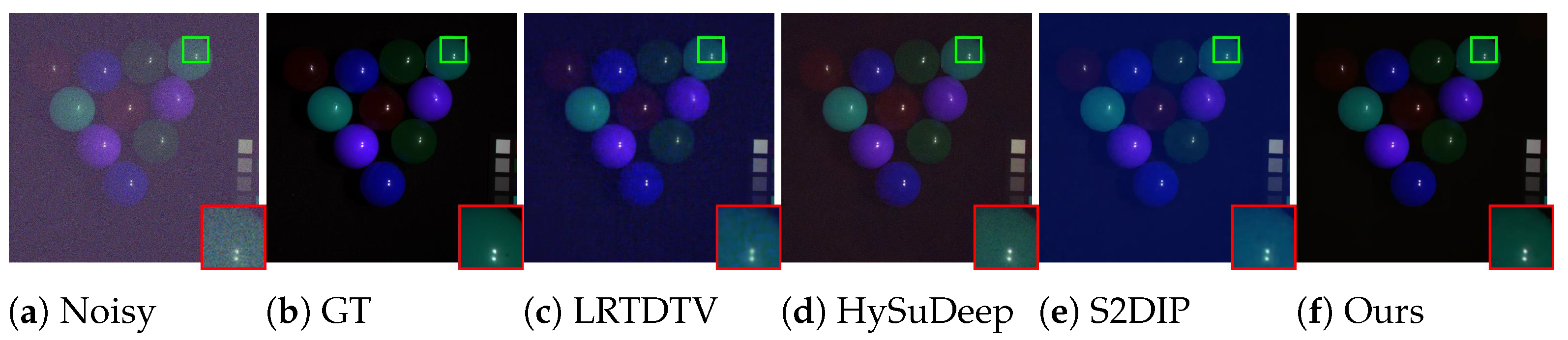
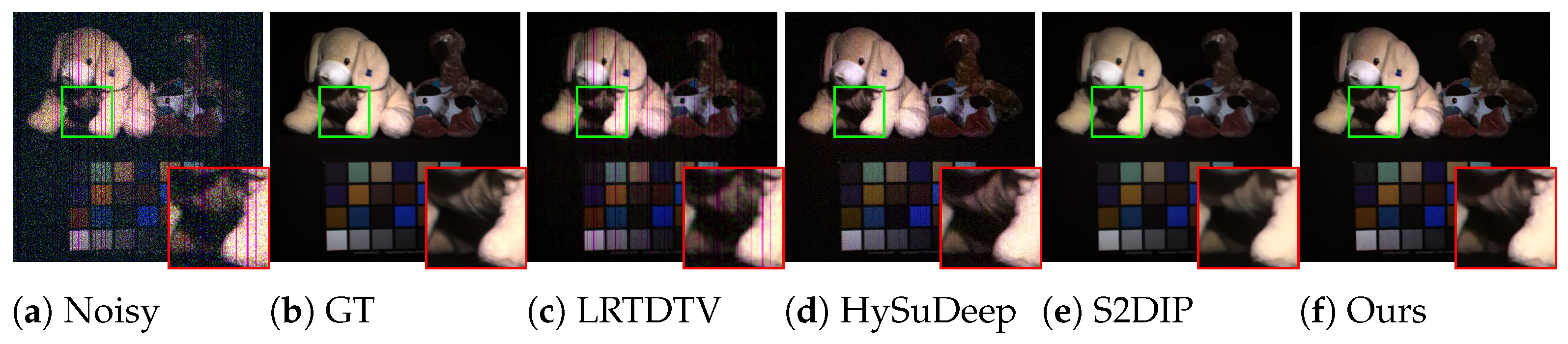
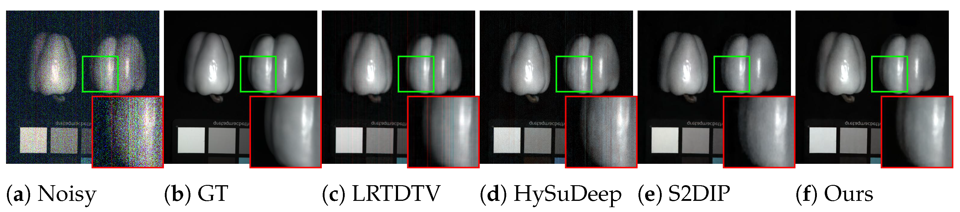
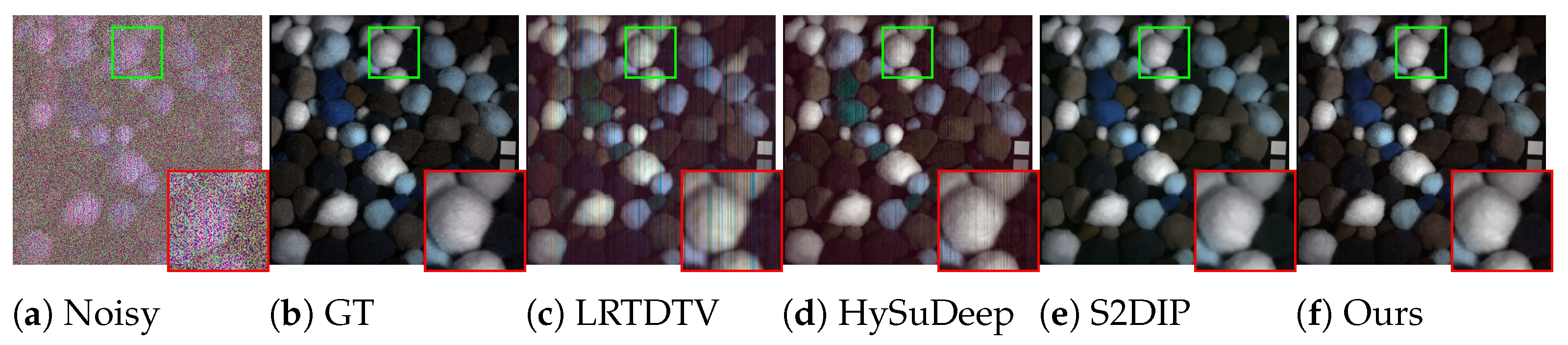
• We demonstrate the applications of the proposed method on various HSI denoising examples, both synthetic and real, under different types of complex noise.

The rest of the paper is organized as follows. Section 2 briefly reviews related work. Section 3 discusses the details of the proposed method, including the probabilistic model and the solving algorithm. Section 4 introduces the experimental results on both synthetic and real noisy HSIs to demonstrate the effectiveness of the proposed method. Then, the paper is concluded in Section 5.

2. Related Work

In this section, we briefly review related studies on the HSI denoising task, which can be roughly categorized into model-driven methods and data-driven ones.

2.1. Model-Driven Methods

Traditionally, HSI denoising methods were mainly developed in a model-driven way, and the key is how to properly specify the fidelity and regularization terms in (2), which correspond to noise assumption and prior knowledge of HSIs, respectively. There are plenty of studies concerning designing the regularization term to impose certain prior knowledge to the clean HSIs. For example, considering the intrinsic correlation between the spectral bands, low-rank models [11,34] have been adopted, and to characterize the correlations between HSI patches, non-local similarity-oriented models [35,36,37] have been developed. In recent studies, TV [38] and its variants have shown their importance in HSI denoising. For example, He et al. [13] introduced TV to characterize the local smoothness in the spatial domain, Wang et al. [14] further took the spectral domain into consideration and proposed the SSTV regularizer, and Peng et al. [27] enhanced the 3D version of TV by deeper investigations on the gradient domain of the HSIs. Recently, motivated by its successful applications in RGB image processing, the DIP [29] was generalized to the HSI version [30] and its potential demonstrated in HSI denoising. Luo et al. [10] went a step further by integrating the TV-type regularizations with the DIP and achieved a remarkable HSI denoising performance. These studies motivate us to consider both the TV and SSTV in our denoising model.

For the noise assumption, a straightforward and most widely used choice is the Gaussian noise, which results in the squared $L_2$-norm as the fidelity term. However, it does not perform well under the sparse noise scenario, such as stripe noise or deadline, that is often encountered in HSIs. Thus, $L_1$-norm is adopted in many previous studies [17,18,19,20], which is often combined with the squared $L_2$-norm for complementarity. Beyond the simple $L_2$-norm and $L_1$-norm, which still do not perfectly fit the real scenarios of noisy HSIs, a noise modeling strategy has been considered. For example, with the simple matrix-based low-rank prior for the clean HSI, Chen et al. [21] modeled the complex noise within real HSIs as a band-wise mixture of Gaussians, and Yue et al. [22] further considered a hierarchical Dirichlet process mixture model for the HSI noise. Then, Ma et al. [23] and Jiang et al. [39] combined the noise modeling strategy with more sophisticated HSI priors, such as self-similarity, tensor-based low-rankness and neural-network-based implicit prior. Those noise modeling methods have demonstrated their ability in precisely characterizing the complex noise structure within real HSIs and thus motivate us to also consider such a methodology.

2.2. Data-Driven Methods

In the last few years, motivated by the success of deep learning (DL) in a wide range of applications, data-driven methods have attracted increasing attention in HSI denoising. The main idea behind this kind of method is to learn a direct mapping from the noisy HSI to its clean counterpart in a data-driven way. In this line of research, the 2D convolutional neural network (CNN) was first considered [6,7] and showed promising performance. Then, for fully exploring both the spatial and spectral information, 3D CNN models were developed [8,40] and have demonstrated their advantages over 2D CNNs. Later, more advanced neural network architectures were introduced to the HSI denoising task, including recurrent neural network [41], U-Net [42], attention mechanism [43] and transformer [44,45]. These data-driven methods generally have a good performance on the HSI denoising task if provided proper training. However, their performance could be limited by the restricted training data, especially when generalizing to real noisy HSIs with unseen types of noise.

In addition to learning a direct noisy-to-clean mapping, the data-driven strategy can also facilitate the HSI denoising in an indirect way. Recently, Rui et al. [25] made a successful attempt in this direction. Specifically, they proposed an approach to efficiently learn a CNN for predicting the weights in the fidelity term of (2). This approach indeed realizes noise modeling for noisy HSI in a data-driven way, which can be simpler and more flexible than the noise modeling techniques discussed before. Thus, we integrate this idea into our denoising model.

3. Proposed Method

In this section, we first propose our probabilistic model for HSI denoising and then present the solving algorithm for the resulted MAP estimation problem.

3.1. Probabilistic Model

Following the observation model (1) for the noisy HSI $\mathcal{Y}$ and placing prior to the clean HSI $\mathcal{X}$, we can simply obtain the probabilistic model in general:

$$p(\mathcal{X},\mathcal{Y})=p(\mathcal{Y}|\mathcal{X})p(\mathcal{X}),$$

(3)

and then realize HSI denoising by estimating the posterior according to Bayesian rule:

$$p(\mathcal{X}|\mathcal{Y})\propto p(\mathcal{Y}|\mathcal{X})p(\mathcal{X}).$$

(4)

Therefore, the key is how to specify the likelihood $p(\mathcal{Y}|\mathcal{X})$, or equivalently the noise distribution $p(\mathcal{E})$, and the prior $p(\mathcal{X})$, which intrinsically correspond to the fidelity term and the regularization term in (2), respectively. In the following, we will discuss our approach for modeling the two terms and the resulting MAP estimation problem.

3.1.1. Noise Modeling

As mentioned in Introduction and Related Work, there are several studies that have specifically considered modeling noise for HSI denoising [21,22,23,24,46], which often use complex distributions. In this work, we use a relatively simpler, while flexible enough, model for the noise, i.e., pixel-wise non-i.i.d. Gaussian. Specifically, denoting $\mathcal{Y}(i,j,k)$ as the $ijk$-th pixel in the noisy HSI cube $\mathcal{Y}$ and, similarly, $\mathcal{X}(i,j,k)$ for $\mathcal{X}$, we propose the following model for the noisy HSI:

$$\begin{array}{c}\hfill \mathcal{Y}(i,j,k)=\mathcal{X}(i,j,k)+\mathcal{E}(i,j,k),\\ \hfill \mathcal{E}(i,j,k)\sim \mathcal{N}(0,1/\mathcal{W}{(i,j,k)}^2),\end{array}$$

(5)

where $\mathcal{N}(\mu ,{\kappa }^{-1})$ denotes the Gaussian distribution with mean $\mu$ and precision $\kappa$, and $\mathcal{W}{(i,j,k)}^2$ is the corresponding precision parameter of the $ijk$-th pixel. Though seemingly simple, this noise model is indeed very flexible, since we can specify different precision parameters for different pixels to approximate very complex noise.

The pixel-wise noise model (5) can then lead to the following likelihood term:

$$p(\mathcal{Y}|\mathcal{X})\propto \exp \left\{-{\displaystyle \frac{1}{2}}{∥\mathcal{W}\odot (\mathcal{Y}-\mathcal{X})∥}_F^2\right\},$$

(6)

where $\mathcal{W}\in {\mathbb{R}}^{h\times w\times b}$ is a weight tensor whose $ijk$-th element is $\mathcal{W}(i,j,k)$. As will be seen later, this form of likelihood results in a weighted least square term in the optimization procedure, which facilitates a simpler solving algorithm.

The final issue in completing the noise model is how to specify the weight tensor $\mathcal{W}$. Here, we follow the strategy by Rui et al. [25], i.e., using a pre-trained neural network to predict $\mathcal{W}$ from the noisy HSI $\mathcal{Y}$ in a data-driven manner, which can make the noise parameters automatically fit the observations.

3.1.2. Prior Modeling

Traditionally, TV [47] and SSTV [17,48] regularizers have shown their effectiveness in HSI denoising, while recently, DIP has also shown its potential for this task [30]. Therefore, following the idea by Luo et al. [10], we incorporate the TV and SSTV with DIP, but in a more concise probabilistic model. Specifically, we define the prior for the clean HSI in the following way:

$$\begin{array}{cc}\hfill \mathcal{X}& =\mathcal{G}(z;\theta ),\hfill \\ \hfill \theta |z& \sim p(\theta |z)\propto \exp \left\{-{\alpha }_1{∥\mathcal{G}(z;\theta )∥}_{\mathrm{TV}}-{\alpha }_2{∥\mathcal{G}(z;\theta )∥}_{\mathrm{SSTV}}\right\},\hfill \\ \hfill z& \sim \mathcal{N}(\mathbf{0};\mathit{I}),\hfill \end{array}$$

(7)

where $\mathcal{G}(·;\theta )$ is a neural network parameterized by $\theta$, $\mathcal{N}(\mathit{\mu };\mathbf{\Sigma })$ denotes the multivariate Gaussian distribution parameterized by $\mathit{\mu }$ and $\mathbf{\Sigma }$, $\mathit{I}$ is the identity matrix, and ${\parallel ·\parallel }_{\mathrm{TV}}$ and ${\parallel ·\parallel }_{\mathrm{TV}}$ are the TV and SSTV, respectively, defined as

$${∥\mathcal{X}∥}_{\mathrm{TV}}={∥{\nabla }_x\mathcal{X}∥}_{{\ell }_1}+{∥{\nabla }_y\mathcal{X}∥}_{{\ell }_1}$$

(8)

and

$${∥\mathcal{X}∥}_{\mathrm{SSTV}}={∥{\nabla }_x({\nabla }_z\mathcal{X})∥}_{{\ell }_1}+{∥{\nabla }_y({\nabla }_z\mathcal{X})∥}_{{\ell }_1},$$

(9)

where ${\parallel ·\parallel }_{{\ell }_1}$ denotes the matrix ${\ell }_1$-norm, i.e., the sum of absolute values of all elements in a matrix, and the derivative tensors ${\nabla }_x\mathcal{X}\in {\mathbb{R}}^{(h-1)\times w\times b}$, ${\nabla }_y\mathcal{X}\in {\mathbb{R}}^{h\times (w-1)\times b}$ and ${\nabla }_z\mathcal{X}\in {\mathbb{R}}^{h\times w\times (b-1)}$ are defined as

$$\left\{\begin{array}{cc}\hfill {\nabla }_x\mathcal{X}(i,j,k)& =\mathcal{X}(i+1,j,k)-\mathcal{X}(i,j,k)\hfill \\ \hfill {\nabla }_y\mathcal{X}(i,j,k)& =\mathcal{X}(i,j+1,k)-\mathcal{X}(i,j,k)\hfill \\ \hfill {\nabla }_z\mathcal{X}(i,j,k)& =\mathcal{X}(i,j,k+1)-\mathcal{X}(i,j,k)\hfill \end{array}\right.$$

(10)

with ${\nabla }_x$, ${\nabla }_y$ and ${\nabla }_z$ being the finite derivative operators on the vertical, horizontal and spectral directions, respectively.

Before proceeding, we briefly explain the nature of the proposed prior model. The first two lines of (7) are indeed a probabilistic reformulation of the parameterization and regularizations adopted by Luo et al. [10]. Specifically, the first line parameterizes the clean HSI $\mathcal{X}$ by a neural network (DIP), and the second line is the probabilistic formulation of the TV and SSTV regularization terms used in [10]. Different from Luo et al. [10], who treat $z$ as a random input, following the standard way of DIP, we consider it as a latent variable and introduce a Gaussian prior (the third line of (7)). As shown in [49], such a strategy can benefit the performance of the DIP-based algorithm. We will further discuss its advantage in the following part and empirically demonstrate it in experiments.

3.1.3. Overall Model and MAP Estimation

Combining (6) and (7), we can obtain the following probabilistic generative model for HSI denoising:

$$\begin{array}{cc}\hfill p(\mathcal{X},\mathcal{Y},z,\theta )=& p(\mathcal{Y}|\mathcal{X})p(\mathcal{X}|z,\theta )p(\theta |z)p(z)\hfill \\ \hfill =& p(\mathcal{Y}|\mathcal{X})\mathbb{I}\left\{\mathcal{X}=\mathcal{G}(z;\theta )\right\}p(\theta |z)p(z)\hfill \\ \hfill =& p(\mathcal{Y}|\mathcal{G}(z;\theta ))p(\theta |z)p(z)\hfill \\ \hfill \propto & \exp \left\{-{\displaystyle \frac{1}{2}}{∥\mathcal{W}\odot (\mathcal{Y}-\mathcal{G}(z;\theta ))∥}_F^2\right\}\hfill \\ \hfill & \exp \left\{-{\alpha }_1{∥\mathcal{G}(z;\theta )∥}_{\mathrm{TV}}-{\alpha }_2{∥\mathcal{G}(z;\theta )∥}_{\mathrm{SSTV}}\right\}\hfill \\ \hfill & \exp \left\{-{\displaystyle \frac{1}{2}}{z}^{T}z\right\}\hfill \end{array}$$

(11)

where $\mathbb{I}\{·\}$ is the indicator function that ensures the event within the curly brackets to be true. Given that $\mathcal{X}$ is indeed represented by $z$ and $\theta$, we can omit the explicit expression of $\mathcal{X}$ in the above joint distribution and write

$$p(\mathcal{X},\mathcal{Y},z,\theta )=p(\mathcal{Y},z,\theta )=p(\mathcal{Y}|\mathcal{G}(z;\theta ))p(\theta |z)p(z).$$

(12)

Then, the posterior of $\theta$ can be obtained by

$$p(\theta |\mathcal{Y})\propto \int p(\mathcal{Y},z,\theta )\mathrm{d}z=\int p(\mathcal{Y}|\mathcal{G}(z;\theta ))p(\theta |z)p(z)\mathrm{d}z,$$

(13)

where we integrate out the latent variable $z$, and $\mathcal{Y}$ is the only observation we have. Then, we can perform MAP estimation to $\theta$:

$$\underset{\theta }{\max }\log \int p(\mathcal{Y}|\mathcal{G}(z;\theta ))p(\theta |z)p(z)\mathrm{d}z.$$

(14)

Once the optimal $\theta$ is obtained, we can recover the estimated clean HSI by

$$\mathcal{X}={\mathbb{E}}_z\left[\mathcal{G}(z;\theta )\right],$$

(15)

where ${\mathbb{E}}_z[·]$ denotes the expectation with respect to the latent variable $z$. Compared with conventional DIP-based methods that only input a single $z$, we can take the expectation to obtain a model-averaged result. This is the key advantage of our proposed probabilistic model, which will be demonstrated in experiments.

3.2. Solving Algorithm for The MAP Estimation

Our goal now is to effectively solve the MAP estimation problem (14). Note that since there exists a complex integral, the analytic form of the objective can not be easily obtained. Therefore, we resort to the MCEM [50] framework to deal with the issue.

3.2.1. Overall EM Process

Following the general EM framework, we iterate between the E-step and M-step to solve the MAP estimation. In the E-step, we construct the surrogate function by taking the expectation with respect to the latent variable $z$:

$$Q(\theta ;\overline{\theta })={\mathbb{E}}_{z|\mathcal{Y},\overline{\theta }}\left[\log p(\mathcal{Y},z,\theta )\right],$$

(16)

where $\overline{\theta }$ denotes the current value of $\theta$. In the M-step, we obtain a new value of $\theta$ by the following optimization:

$$\underset{\theta }{\max }Q(\theta ;\overline{\theta })$$

(17)

Note that the expectation in the E-step cannot be exactly computed due to the analytically intractable posterior $p(z|\mathcal{Y},\overline{\theta })$ and the complex form of $p(\mathcal{Y},z,\theta )$, and thus, we use the Monte Carlo strategy to approximate it. Once the expectation is properly approximated, we apply the ADMM to solve the optimization problem in the M-step. The whole process is summarized in Algorithm 1, and the details of the two alternative steps are discussed in the following parts.

Algorithm 1 HSI denoising by noise modeling and DIP

Input:  Noisy HSI $\mathcal{Y}$, pre-training weighting function $f(·)$, hyper-parameters $T,\delta ,\mu$   1: Randomly initialize $\theta$, $\overline{z}$${\Lambda }_i=0(i=1,2,3,4)$   2: Compute weight tensor $\mathcal{W}=f(\mathcal{Y})$   3: while not converged do   4:     $\overline{\theta }:=\theta$, $z^{(0)}:=\overline{z}$   5:     for $t=0,·,T-1$ do   6:           $z^{(t+1)}=z^{(t)}+{\displaystyle \frac{{\delta }^2}{2}}{\nabla }_z{\left.\log p(\mathcal{Y},z,\overline{\theta })\right|}_{z=z^{(t)}}+\delta {\xi }^{(t)}$   7:     end for   8:     $\overline{z}:=z^{(T)}$   9:    Update ${\mathcal{V}}_i(i=1,2,3,4)$ by (28)   10:   Update $\theta$ by (30)   11:   Update ${\Lambda }_i(i=1,2,3,4)$ by (31)   12: end while Output:  Denoised HSI $\widehat{\mathcal{X}}=\mathcal{G}(\overline{z};\theta )$

3.2.2. Monte Carlo E-Step for Updating Latent Variable

To apply the Monte Carlo approximation to the expectation in (16), we first need to (approximately) sample $z$ from the distribution $p(z|\mathcal{Y},\overline{\theta })$. There are various ways of performing such sampling, and we adopt the Langevin dynamics [32] due to its simplicity. Specifically, the sampling process can be written as

$$z^{(\tau +1)}=z^{(\tau )}+{\displaystyle \frac{{\delta }^2}{2}}{\nabla }_z{\left.\log p(\mathcal{Y},z,\overline{\theta })\right|}_{z=z^{(\tau )}}+\delta {\xi }^{(\tau )},$$

(18)

where $\tau$ denotes the time step for Langevin dynamics, $\delta$ is the step size, and $\xi$ the Gaussian white noise. According to (11), $\log p(\mathcal{Y},z,\overline{\theta })$ can be evaluated as

$$\log p(\mathcal{Y},z,\overline{\theta })=-{\displaystyle \frac{1}{2}}{∥\mathcal{W}\odot (\mathcal{Y}-\mathcal{G}(z;\theta ))∥}_F^2-{\alpha }_1{∥\mathcal{G}(z;\theta )∥}_{\mathrm{TV}}-{\alpha }_2{∥\mathcal{G}(z;\theta )∥}_{\mathrm{SSTV}}-{\displaystyle \frac{1}{2}}{z}^{T}z+C_1,$$

(19)

where $C_1$ is a constant irrelevant to $z$, and thus, its gradient with respect to $z$ can be readily calculated using automatic differentiation provided by modern deep learning packages, such as PyTorch [51].

With a set of sampled $z$s, denoted as $\{z_1,\cdots ,z_L\}$, we can then use the Monte Carlo method to approximate $Q(\theta ;\overline{\theta })$:

$$Q(\theta ;\overline{\theta })\approx {\displaystyle \frac{1}{L}}\sum _{l=1}^L\log p(\mathcal{Y},z_l,\theta ).$$

(20)

Practically, we can even let $L=1$ [52,53] and use the following simplified approximation:

$$Q(\theta ;\overline{\theta })\approx \log p(\mathcal{Y},\overline{z},\theta )\triangleq \widehat{Q}(\theta ;\overline{\theta }),$$

(21)

where $\overline{z}=z^{(T)}$ with T being the total number of Langevin steps.

3.2.3. M-Step for Updating DIP Parameter

With the approximated surrogate function $\widehat{Q}(\theta ;\overline{\theta })$ obtained in the E-step, we then update the DIP parameter in the M-step by the following optimization:

$$\underset{\theta }{\max }\widehat{Q}(\theta ;\overline{\theta }),$$

(22)

where

$$\widehat{Q}(\theta ;\overline{\theta })=-{\displaystyle \frac{1}{2}}{∥\mathcal{W}\odot (\mathcal{Y}-\mathcal{G}(\overline{z};\theta ))∥}_F^2-{\alpha }_1{∥\mathcal{G}(\overline{z};\theta )∥}_{\mathrm{TV}}-{\alpha }_2{∥\mathcal{G}(\overline{z};\theta )∥}_{\mathrm{SSTV}}+C_2,$$

(23)

with $C_2$ being a constant irrelevant to $\theta$. This optimization is indeed equivalent to

$$\underset{\theta }{\min }{\displaystyle \frac{1}{2}}{∥\mathcal{W}\odot (\mathcal{Y}-\mathcal{G}(\overline{z};\theta ))∥}_F^2+{\alpha }_1{∥\mathcal{G}(\overline{z};\theta )∥}_{\mathrm{TV}}+{\alpha }_2{∥\mathcal{G}(\overline{z};\theta )∥}_{\mathrm{SSTV}}.$$

(24)

Optimization (24) can be solved by the ADMM [33]. Specifically, we can first introduce four auxiliary variables to reformulate the optimization model (24) as

$$\begin{array}{cc}\hfill & \underset{\theta }{\min }\parallel \mathcal{W}\odot (\mathcal{Y}-\mathcal{G}(\overline{z};\theta )){\parallel }_F^2+{\alpha }_1(\parallel V_1{\parallel }_{{\ell }_1}+\parallel V_2{\parallel }_{{\ell }_1})+{\alpha }_2(\parallel V_3{\parallel }_{{\ell }_1}+\parallel V_4{\parallel }_{{\ell }_1})\hfill \\ \hfill s.t.& V_1={\nabla }_x(\mathcal{G}(\overline{z};\theta )),V_2={\nabla }_y(\mathcal{G}(\overline{z};\theta )),V_3={\nabla }_x{\nabla }_z(\mathcal{G}(\overline{z};\theta )),V_4={\nabla }_y{\nabla }_z(\mathcal{G}(\overline{z};\theta )).\hfill \end{array}$$

(25)

Then, the augmented Lagrangian function can be written as follows:

$$\begin{array}{cc}\hfill L_{\mu }(\overline{z},\theta ,{\mathcal{V}}_1,{\mathcal{V}}_2,{\mathcal{V}}_3,{\mathcal{V}}_4)=& {∥\mathcal{W}\odot (\mathcal{Y}-\mathcal{G}(\overline{z};\theta ))∥}_F^2+{\alpha }_1(\parallel {\mathcal{V}}_1{\parallel }_{{\ell }_1}+\parallel {\mathcal{V}}_2{\parallel }_{{\ell }_1})\hfill \\ \hfill & +{\alpha }_2(\parallel {\mathcal{V}}_3{\parallel }_{{\ell }_1}+\parallel {\mathcal{V}}_4{\parallel }_{{\ell }_1})+{\alpha }_3{\parallel S\parallel }_{{\ell }_1}\hfill \\ \hfill & +{\displaystyle \frac{\mu }{2}}{\parallel {\nabla }_x(\mathcal{G}(\overline{z};\theta ))-{\mathcal{V}}_1\parallel }_F^2+\langle {\Lambda }_1,{\nabla }_x(\mathcal{G}(\overline{z},\theta ))-{\mathcal{V}}_1\rangle \hfill \\ \hfill & +{\displaystyle \frac{\mu }{2}}{\parallel {\nabla }_y(\mathcal{G}(\overline{z};\theta ))-{\mathcal{V}}_2\parallel }_F^2+\langle {\Lambda }_2,{\nabla }_y(G(\overline{z},\theta ))-{\mathcal{V}}_2\rangle \hfill \\ \hfill & +{\displaystyle \frac{\mu }{2}}{\parallel {\nabla }_x{\nabla }_z(\mathcal{G}(\overline{z};\theta ))-{\mathcal{V}}_3\parallel }_F^2+\langle {\Lambda }_3,{\nabla }_x{\nabla }_z(\mathcal{G}(\overline{z},\theta ))-{\mathcal{V}}_3\rangle \hfill \\ \hfill & +{\displaystyle \frac{\mu }{2}}{\parallel {\nabla }_y{\nabla }_z(\mathcal{G}(\overline{z};\theta ))-{\mathcal{V}}_4\parallel }_F^2+\langle {\Lambda }_4,{\nabla }_y{\nabla }_z(\mathcal{G}(\overline{z},\theta ))-{\mathcal{V}}_4\rangle \hfill \end{array}$$

(26)

where $\mu$ is the penalty parameter, and ${\left\{{\Lambda }_i\right\}}_{i=1}^4$ are the Lagrangian multipliers. By ADMM, the problem is then decomposed into the following subproblems:

$\mathcal{V}$-subproblems: The subproblems for updating ${\left\{{\mathcal{V}}_i\right\}}_{i=1}^4$ are

$$\left\{\begin{array}{cc}\hfill & \underset{{\mathcal{V}}_1}{\min }{\alpha }_1\parallel {\mathcal{V}}_1{\parallel }_{{\ell }_1}+{\displaystyle \frac{\mu }{2}}{\parallel {\nabla }_x(\mathcal{G}(\overline{z};\theta ))+{\displaystyle \frac{{\Lambda }_1}{\mu }}-{\mathcal{V}}_1\parallel }_F^2\hfill \\ \hfill & \underset{{\mathcal{V}}_2}{\min }{\alpha }_1\parallel {\mathcal{V}}_2{\parallel }_{{\ell }_1}+{\displaystyle \frac{\mu }{2}}{\parallel {\nabla }_x(\mathcal{G}(\overline{z};\theta ))+{\displaystyle \frac{{\Lambda }_2}{\mu }}-{\mathcal{V}}_2\parallel }_F^2\hfill \\ \hfill & \underset{{\mathcal{V}}_3}{\min }{\alpha }_2\parallel {\mathcal{V}}_3{\parallel }_{{\ell }_1}+{\displaystyle \frac{\mu }{2}}{\parallel {\nabla }_x{\nabla }_z(\mathcal{G}(\overline{z};\theta ))+{\displaystyle \frac{{\Lambda }_3}{\mu }}-{\mathcal{V}}_3\parallel }_F^2\hfill \\ \hfill & \underset{{\mathcal{V}}_4}{\min }{\alpha }_2\parallel {\mathcal{V}}_4{\parallel }_{{\ell }_1}+{\displaystyle \frac{\mu }{2}}{\parallel {\nabla }_x{\nabla }_z(\mathcal{G}(\overline{z};\theta ))+{\displaystyle \frac{{\Lambda }_4}{\mu }}-{\mathcal{V}}_4\parallel }_F^2\hfill \end{array}\right.$$

(27)

which can be directly solved by

$$\left\{\begin{array}{cc}\hfill & {\mathcal{V}}_1={\mathrm{soft}}_{{\displaystyle \frac{{\alpha }_1}{\mu }}}\left({\nabla }_x(\mathcal{G}(\overline{z};\theta ))+{\displaystyle \frac{{\Lambda }_1}{\mu }}\right)\hfill \\ \hfill & {\mathcal{V}}_2={\mathrm{soft}}_{{\displaystyle \frac{{\alpha }_1}{\mu }}}\left({\nabla }_y(\mathcal{G}(\overline{z};\theta ))+{\displaystyle \frac{{\Lambda }_2}{\mu }}\right)\hfill \\ \hfill & {\mathcal{V}}_3={\mathrm{soft}}_{{\displaystyle \frac{{\alpha }_2}{\mu }}}\left({\nabla }_x{\nabla }_z(\mathcal{G}(\overline{z};\theta ))+{\displaystyle \frac{{\Lambda }_3}{\mu }}\right)\hfill \\ \hfill & {\mathcal{V}}_4={\mathrm{soft}}_{{\displaystyle \frac{{\alpha }_2}{\mu }}}\left({\nabla }_y{\nabla }_z(\mathcal{G}(\overline{z};\theta ))+{\displaystyle \frac{{\Lambda }_4}{\mu }}\right)\hfill \end{array}\right.$$

(28)

in which ${\mathrm{soft}}_{\lambda }(·)$ is the soft-thresholding operator defined as:

$${\mathrm{soft}}_{\lambda }(x)=\mathrm{sign}(x)\max \left\{\right|x|-\lambda ,0\},$$

(29)

and operates element-wise.

$\mathit{\theta }$-subproblem: The subproblem of $\theta$ can be written as follows:

$$\begin{array}{cc}\hfill \underset{\theta }{\min }& \parallel \mathcal{W}\odot (\mathcal{Y}-\mathcal{G}(\overline{z};\theta )){\parallel }_F^2+{\displaystyle \frac{\mu }{2}}(\parallel {\nabla }_x(\mathcal{G}(\overline{z};\theta ))-{\mathcal{V}}_1+{\displaystyle \frac{{\Lambda }_1}{\mu }}{\parallel }_F^2+\parallel {\nabla }_y(\mathcal{G}(\overline{z};\theta ))-{\mathcal{V}}_2\hfill \\ \hfill & +{\displaystyle \frac{{\Lambda }_2}{\mu }}{\parallel }_F^2+\parallel {\nabla }_x{\nabla }_z(\mathcal{G}(\overline{z};\theta ))-{\mathcal{V}}_3+{\displaystyle \frac{{\Lambda }_3}{\mu }}{{\parallel }_F^2+{\nabla }_y{\nabla }_z(\mathcal{G}(\overline{z};\theta ))-{\mathcal{V}}_4+{\displaystyle \frac{{\Lambda }_4}{\mu }}\parallel }_F^2).\hfill \end{array}$$

(30)

Though it cannot be analytically solved, we can update $\theta$ with respect to this optimization by several gradient steps, using solvers like Adam [54], which can be easily implemented by virtue of deep learning packages, such as PyTorch [51].

$\mathbf{\Lambda }$ updating: The Lagrangian multipliers ${\left\{{\Lambda }_i\right\}}_{i=1}^4$ can then be updated by

$$\left\{\begin{array}{cc}\hfill & {\Lambda }_1:={\Lambda }_1+\mu \left({\nabla }_x(\mathcal{G}(\overline{z};\theta ))-{\mathcal{V}}_1\right)\hfill \\ \hfill & {\Lambda }_2:={\Lambda }_2+\mu \left({\nabla }_y(\mathcal{G}(\overline{z};\theta ))-{\mathcal{V}}_2\right)\hfill \\ \hfill & {\Lambda }_3:={\Lambda }_3+\mu \left({\nabla }_x{\nabla }_z(\mathcal{G}(\overline{z};\theta ))-{\mathcal{V}}_3\right)\hfill \\ \hfill & {\Lambda }_3:={\Lambda }_3+\mu \left({\nabla }_x{\nabla }_z(\mathcal{G}(\overline{z};\theta ))-{\mathcal{V}}_4\right)\hfill \end{array}.\right.$$

(31)

4. Experiments

In this section, we conduct both simulation and real case experiments to verify the effectiveness of the proposed method.

4.1. Experimental Settings

4.1.1. Datasets

For a comprehensive comparison, we conduct experiments on clean HSI datasets with simulated noise and noisy HSI datasets from real scenarios.

For the sythetic data, we artificially add noise of different types to different HSI datasets to generate the noisy HSIs. Specifically, we consider two commonly adopted HSI datasets:

• CAVE: The Columbia Imaging and Vision Laboratory (CAVE) dataset [55] contains 31 HSIs with real-world objects in indoor scenarios. Each HSI in this dataset has 31 bands and a spatial size of $512\times 512$.
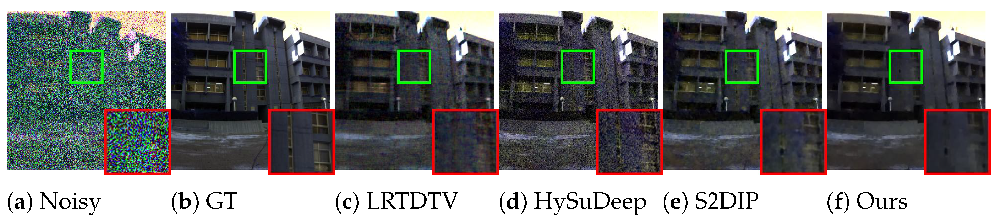
• ICVL: The Ben-Gurion University Interdisiplinary Computational Vision Laboratory (ICVL) dataset [56] is composed of 201 HSIs with a spatial resolution $1392\times 1200$ over 519 spectra. The HSIs in this dataset are captured on natural outdoor scenes with complex background structures. In our experiments, we select 11 HSIs for comparison.

Following the previous study [21], we consider five different types of complex noise:

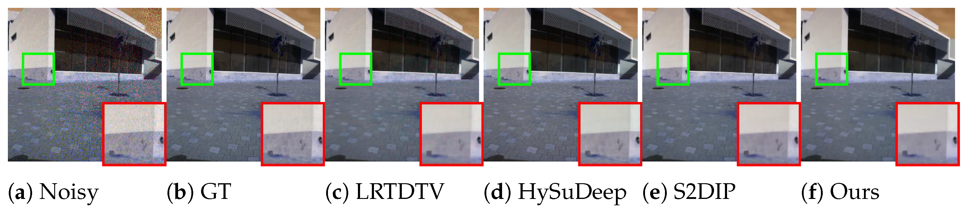
• Case 1 (Non-i.i.d Gaussian): The entire HSI is corrupted by the zero-mean Gaussian noise with variance 10–70 for all bands.
• Case 2 (Gaussian + Impulse): In addition to the Gaussian noise in Case 1, 10 bands of each HSI are randomly selected and added to impulse noise, whose ratio is between $5\%$ and $20\%$.
• Case 3 (Gaussian + Deadline): In addition to the Gaussian noise in Case 1, 10 bands of each HSI are randomly selected and added to deadline noise, whose ratio is between $5\%$ and $20\%$.
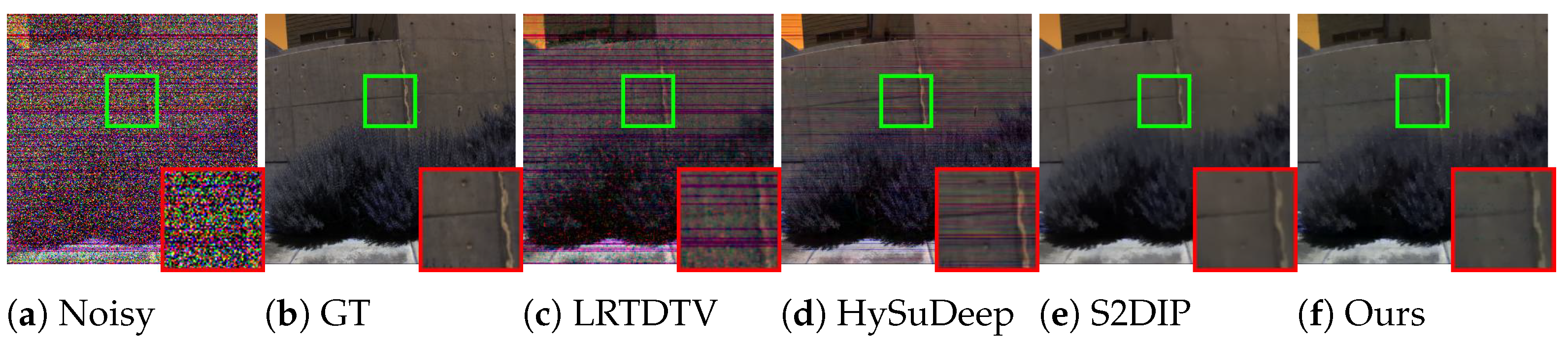
• Case 4 (Gaussian + Stripe): In addition to the Gaussian noise in Case 1, 10 bands of each HSI are randomly selected and added to stripe noise, whose ratio is between $5\%$ and $20\%$.
• Case 5 (Mixture): Each band of HSI is randomly corrupted with at least one type of noise as that in the aforementioned cases.

For the real data, we consider two HSIs of real-earth observations, i.e., Indian Pines (https://purr.purdue.edu/publications/1947/1, accessed on 10 May 2024) with the size of $145\times 145\times 220$ and Urban with the size of $307\times 307\times 221$. Due to the complex environments of the acquisition process, the noise contained in these two HSIs has complex structures, as shown in Section 4.3.

4.1.2. Compared Methods and Evaluation Metrics

In the experiments, we compare our proposed method with three representative methods, including LRTDTV [14], a traditional model-based method using low-rank and TV as regularization; HySuDeep [57], which uses a plug-in CNN prior in the subspace learning-based denoising procedure; and S2DIP [10], which combines the DIP with TV-based prior.

For quantitative evaluation, we consider four metrics: Peak Signal-to-Noise Ratio (PSNR), Feature Similarity Index (FSIM) [58], Erreur Relative Globale Adimensionnelle de Synthèse (ERGAS) [59] and Spectral Angle Mapper (SAM) [60]. Among the four, PSNR and FSIM are metrics for general image quality assessment, while ERGAS and SAM are metrics specifically designed for HSIs.

4.1.3. Implementation Details

There are several implementation details which should be described concerning the proposed algorithm. The first is about the pre-trained network for predicting the weight tensor $\mathcal{W}$. In the experiments, following [25], we use a CNN pre-trained on 10,000 noisy HSI patches extracted and augmented from the CAVE datasets, under the matrix factorization (MF) model. Albeit relatively simpler to train, this pre-trained CNN has been shown to be able to generalize to other HSI denoising models other than MF and also empirically works well in our model.

There are several hyper-parameters in our algorithm which should also be discussed. First, there are two balance parameters ${\alpha }_1$ and ${\alpha }_2$ in our probabilistic model (11), and we simply set both of them to $0.012$. Then, for the hyper-parameters in Algorithm 1, i.e., T, $\delta$ and $\mu$, we set them as 5, $0.1$ and $0.12$, respectively. Note that though they work well in our experiments, those hyper-parameters are not optimized.

For other competing methods, we follow the recommendations by the authors of the corresponding papers.

4.2. Results on the Synthetic Data

The quantitative results on the two datasets with five types of noise are summarized in

Table 1. Quantitive results of all competing methods on the CAVE dataset. The best performance in each noise case is highlighted in bold.

Case	Method	PSNR	FSIM	ERGAS	SAM
Gaussian	LRTDTV	39.8796	0.9779	4.0462	0.0674
	HySuDeep	40.1336	0.9848	4.58236	0.0646
	S2DIP	41.8339	0.9888	2.8531	0.0483
	Ours	41.5929	0.9862	2.7408	0.0469
Impulse	LRTDTV	34.4736	0.9284	7.1868	0.1180
	HySuDeep	30.4910	0.9170	12.5340	0.1761
	S2DIP	37.4550	0.9686	4.5624	0.0788
	Ours	37.2922	0.9707	4.4757	0.0762
Deadline	LRTDTV	32.8379	0.9192	10.2393	0.1427
	HySuDeep	30.5410	0.8218	11.7132	0.1754
	S2DIP	37.0793	0.9668	4.7088	0.0818
	Ours	36.9659	0.9669	4.8187	0.0809
Stripe	LRTDTV	34.6507	0.9284	6.9978	0.1178
	HySuDeep	31.2546	0.9175	10.8651	0.1650
	S2DIP	38.1461	0.9627	4.0421	0.0703
	Ours	37.4689	0.9720	4.3060	0.0720
Mixture	LRTDTV	35.0809	0.9449	9.4196	0.1262
	HySuDeep	35.5482	0.9575	8.0436	0.1053
	S2DIP	39.6789	0.9815	3.5289	0.0611
	Ours	40.2142	0.9822	3.2595	0.0563

and

Table 2. Quantitive results of all competing methods on the ICVL dataset. The best performance in each noise case is highlighted in bold.

Case	Method	PSNR	FSIM	ERGAS	SAM
Gaussian	LRTDTV	27.0421	0.9241	14.0443	0.1300
	HySuDeep	27.2292	0.9478	14.1620	0.1790
	S2DIP	30.2844	0.9613	10.1397	0.0934
	Ours	30.2307	0.9341	8.2538	0.0818
Impulse	LRTDTV	22.0450	0.8469	19.7787	0.2020
	HySuDeep	22.9223	0.8898	17.4486	0.2149
	S2DIP	28.3008	0.9288	8.7353	0.1050
	Ours	28.2520	0.9148	9.8538	0.0937
Deadline	LRTDTV	24.4003	0.8558	15.3513	0.1746
	HySuDeep	23.9010	0.8780	15.0186	0.2036
	S2DIP	26.9224	0.8749	11.2969	0.1058
	Ours	27.9537	0.9089	10.5811	0.0968
Stripe	LRTDTV	23.6814	0.8723	15.7636	0.1757
	HySuDeep	23.1673	0.8885	15.5463	0.2043
	S2DIP	28.1406	0.9309	9.8148	0.1054
	Ours	28.9598	0.9119	9.1531	0.0955
Mixture	LRTDTV	23.5957	0.8631	20.1767	0.1893
	HySuDeep	24.2909	0.9028	17.1100	0.1889
	S2DIP	28.2247	0.9080	10.1001	0.0907
	Ours	27.2590	0.9086	15.0000	0.1263

, respectively. It can be seen that the proposed method consistently performs among the best two in all noise settings on the two datasets, with respect to all the four metrics which demonstrate the effectiveness of it. Regarding the metrics specifically designed for HSIs, i.e., ERGAS and SAM, the effectiveness of the proposed method is more clear. Specifically, it achieves the best performance with respect to SAM in all noise cases on Cave and in four cases on ICVL.

For a more intuitive comparison, we show example visual results on Cave in Figure 1, Figure 2, Figure 3, Figure 4 and Figure 5 and on ICVL in Figure 6, Figure 7, Figure 8, Figure 9 and Figure 10, for all noise cases, where the pseudo color images are constructed by three randomly selected bands from the corresponding HSI. It can be seen from these figures that, in all noise cases, our proposed method can consistently remove noise as much as possible, while retaining more or a comparable amount of details of the HSIs. In comparison, other methods either do not satisfactorily remove the noise, or produce color distortion, especially on the CAVE dataset. For example, we can see from Figure 2 that although S2DIP can remove more noise than LRTDTV and HySuDeep, it produces a severe color distortion compared with the proposed method. It is also observed that the visual results of the proposed method on the ICVL dataset are not as good as on CAVE. This can be attributed to the training of the network for predicting the weight tensor $\mathcal{W}$. Specifically, this network is pre-trained on the patches extracted from the CAVE dataset following [25], and thus, it could be most suited to working on the CAVE dataset and may be less effective in generalizing to ICVL. We believe that this issue could be alleviated by increasing the diversity of the training data to pre-train this network.

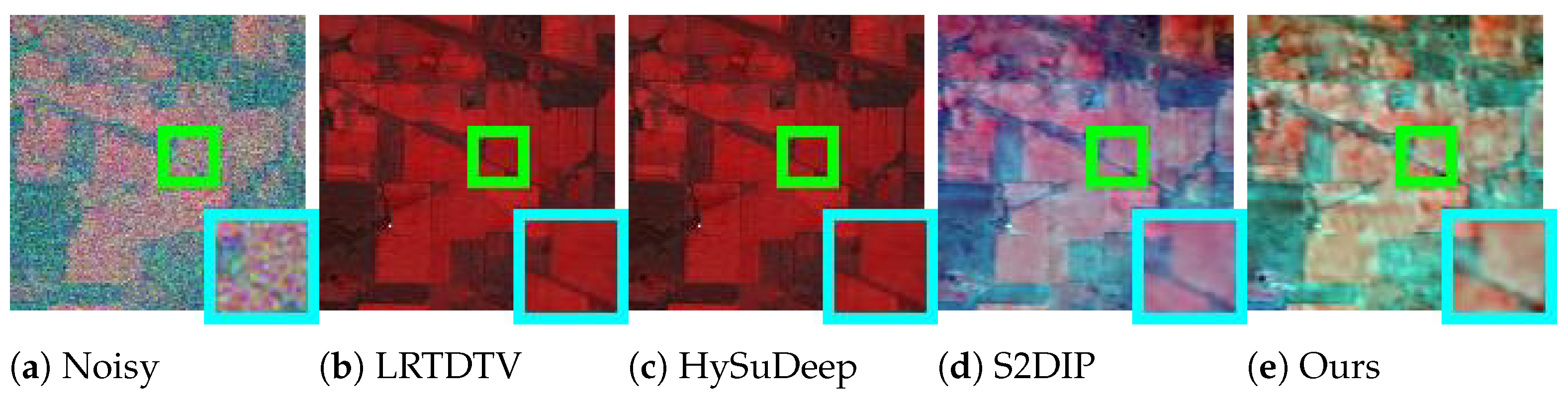
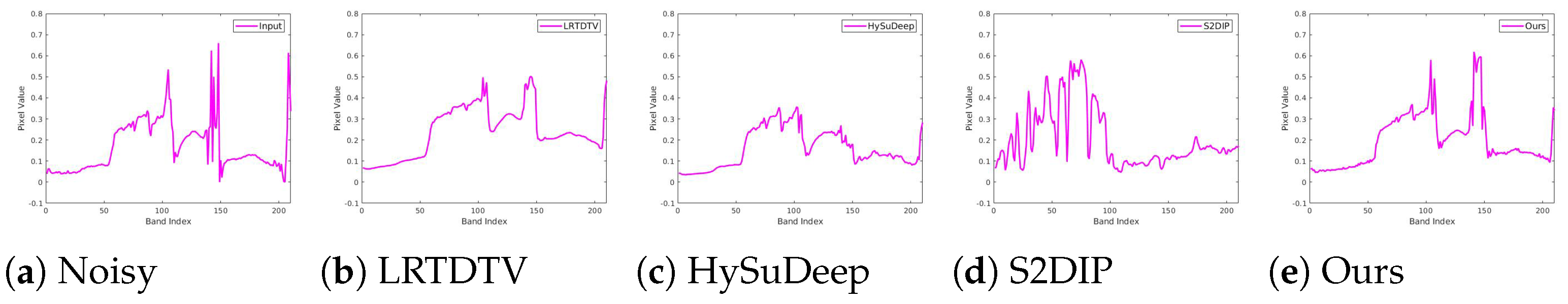
4.3. Experiments on the Real HSIs

Since no groundtruths are available for real noisy HSIs, the quantitative metrics cannot be computed. Therefore, we visualize the results in Figure 11 and Figure 12 for comparison, and the promising performance of the proposed method can be clearly observed. Specifically, for the IndianPines, HSI shown in Figure 11, the results of LRTDTV and HySuDeep have severe color bias, indicating that the two methods fail to recover the spectral information; in comparison, both S2DIP and the proposed method can better recover the HSI. For the Urban HSI shown in Figure 12, we can see that both LRTDTV and HySuDeep fail to remove the stripe noise, while the proposed method can not only completely remove the complex noise but also better keep the spectral information. Compared with S2DIP, the proposed method obtains the result with less color bias. For a more comprehensive comparison, we also show the spectral signatures of pixels from the two HSIs in Figure 13 and Figure 14. We can see that LRTDTV and HySuDeep tend to oversmooth the spectral information, while S2DIP may generate unexpected fluctuations on the Urban HSI. In comparison, the spectral signatures by the proposed method are relatively better on the Urban HSI and comparatively as good as that of S2DIP on the IndianPines HSI.

4.4. More Analyses

In this part, we provide more analyses about the proposed method, including an ablation study on its components, computational complexity and empirical convergence.

4.4.1. Ablation Study

There are mainly three key components in our HSI denoising method, i.e., the pixel-wise noise modeling, the TV-oriented DIP and the EM process, and we thus conduct ablation studies to show their effects. Specifically, we consider two simplified variants of our model, i.e, removing the TV and SSTV regularization and treating the DIP input $z$ as random noise without the E-step update, respectively. Then, we apply these two variants, together with the full model and the S2DIP method, to the CAVE dataset with mixture noise. The results are shown in

Table 3. Results of the ablation study on the CAVE dataset with mixture noise.

Setting	PSNR	FSIM	ERGAS	SAM
w/o TV terms	38.2576	0.9659	4.3830	0.0712
w/o E-step	40.0899	0.9805	3.3132	0.0567
S2DIP	39.6789	0.9815	3.5289	0.0611
Ours	40.2142	0.9822	3.2595	0.0563

. It can be seen that all the components contribute to the final promising performance of the proposed method, specifically ignoring either the TV regularization and the E-step results in a clear performance drop. In addition, considering that the only difference between the setting “w/o E-step” and S2DIP is the fidelity term, the effectiveness of the pixel-wise noise modeling in our method is also evidently substantiated.

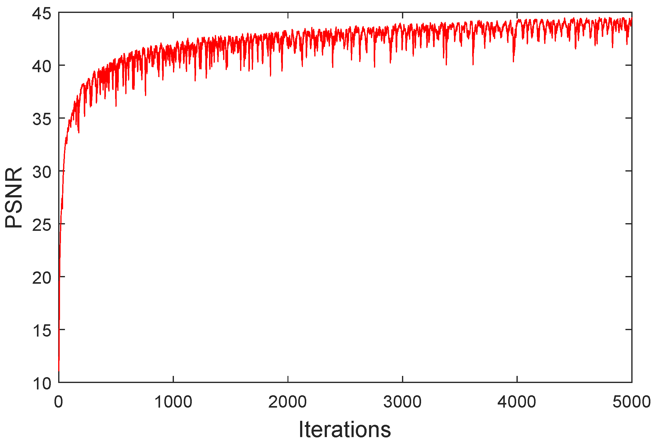
4.4.2. Computational Complexity and Convergence

Since the proposed algorithm adopts the similar DIP and TV regularization terms, its computational complexity is similar to that of S2DIP, despite the SGLD updates in the E-step. Here, we report in

Table 4. Empirical computational complexity comparison between the proposed method and S2DIP. The evaluations were conducted using a NVIDIA RTX 2080 Ti GPU.

Method	Time per HSI (s)	Time per Iteration (s)
S2DIP	692.8	0.23
Ours	987.4	0.33

the empirical running times of the two methods on the CAVE dataset, within which the size of the HSIs is $512\times 512\times 31$ (Since the other two methods were implemented without GPU acceleration, we do not compare with them).

Due to the complex form of the optimization procedure of our method, a theoretical analysis of its convergence is difficult. Therefore, we have empirically shown in Figure 15 the convergence behavior of the proposed algorithm on the Balloon HSI from the CAVE dataset under the mixture noise case. It can be seen that the proposed method can converge to a promising solution with an affordable number of iterations.

5. Conclusions

In this paper, we have proposed a new model-driven HSI denoising method. Specifically, we have presented a unified probabilistic model that integrates both the pixel-wise non-i.i.d Gaussian noise assumption and the TV-oriented DIP for better noise and prior modeling. Then, an MCEM-type algorithm has been designed for solving the resulting MAP estimation problem, in which the SGLD and the ADMM algorithms have been adopted for the E-step and the M-step, respectively. A series of experiments on both synthetic and real noisy HSI datasets have been conducted to verify the effectiveness of the proposed method. Specifically, the proposed method shows promising performance on various complex noise cases, especially on the real noisy HSIs. In the future, we will try to further improve the noise and prior modeling for the HSIs by virtue of the deep generative models, such as GAN [61] and DDPM [62].

References

1. Khan, M.J.; Khan, H.S.; Yousaf, A.; Khurshid, K.; Abbas, A. Modern trends in hyperspectral image analysis: A review. IEEE Access 2018, 6, 14118–14129. [Google Scholar] [CrossRef]
2. Stuart, M.B.; McGonigle, A.J.; Willmott, J.R. Hyperspectral imaging in environmental monitoring: A review of recent developments and technological advances in compact field deployable systems. Sensors 2019, 19, 3071. [Google Scholar] [CrossRef]
3. Shimoni, M.; Haelterman, R.; Perneel, C. Hypersectral imaging for military and security applications: Combining myriad processing and sensing techniques. IEEE Geosci. Remote Sens. Mag. 2019, 7, 101–117. [Google Scholar] [CrossRef]
4. Okada, N.; Maekawa, Y.; Owada, N.; Haga, K.; Shibayama, A.; Kawamura, Y. Automated identification of mineral types and grain size using hyperspectral imaging and deep learning for mineral processing. Minerals 2020, 10, 809. [Google Scholar] [CrossRef]
5. Khan, U.; Paheding, S.; Elkin, C.P.; Devabhaktuni, V.K. Trends in deep learning for medical hyperspectral image analysis. IEEE Access 2021, 9, 79534–79548. [Google Scholar] [CrossRef]
6. Yuan, Q.; Zhang, Q.; Li, J.; Shen, H.; Zhang, L. Hyperspectral image denoising employing a spatial–spectral deep residual convolutional neural network. IEEE Trans. Geosci. Remote Sens. 2018, 57, 1205–1218. [Google Scholar] [CrossRef]
7. Chang, Y.; Yan, L.; Fang, H.; Zhong, S.; Liao, W. HSI-DeNet: Hyperspectral image restoration via convolutional neural network. IEEE Trans. Geosci. Remote Sens. 2018, 57, 667–682. [Google Scholar] [CrossRef]
8. Dong, W.; Wang, H.; Wu, F.; Shi, G.; Li, X. Deep spatial–spectral representation learning for hyperspectral image denoising. IEEE Trans. Comput. Imaging 2019, 5, 635–648. [Google Scholar] [CrossRef]
9. Zhuang, L.; Ng, M.K. FastHyMix: Fast and parameter-free hyperspectral image mixed noise removal. IEEE Trans. Neural Netw. Learn. Syst. 2021, 34, 4702–4716. [Google Scholar] [CrossRef]
10. Luo, Y.S.; Zhao, X.L.; Jiang, T.X.; Zheng, Y.B.; Chang, Y. Hyperspectral mixed noise removal via spatial-spectral constrained unsupervised deep image prior. IEEE J. Sel. Top. Appl. Earth Obs. Remote Sens. 2021, 14, 9435–9449. [Google Scholar] [CrossRef]
11. Zhang, H.; He, W.; Zhang, L.; Shen, H.; Yuan, Q. Hyperspectral image restoration using low-rank matrix recovery. IEEE Trans. Geosci. Remote Sens. 2013, 52, 4729–4743. [Google Scholar] [CrossRef]
12. He, W.; Zhang, H.; Zhang, L.; Shen, H. Hyperspectral image denoising via noise-adjusted iterative low-rank matrix approximation. IEEE J. Sel. Top. Appl. Earth Obs. Remote Sens. 2015, 8, 3050–3061. [Google Scholar] [CrossRef]
13. He, W.; Zhang, H.; Zhang, L.; Shen, H. Total-variation-regularized low-rank matrix factorization for hyperspectral image restoration. IEEE Trans. Geosci. Remote Sens. 2015, 54, 178–188. [Google Scholar] [CrossRef]
14. Wang, Y.; Peng, J.; Zhao, Q.; Leung, Y.; Zhao, X.L.; Meng, D. Hyperspectral image restoration via total variation regularized low-rank tensor decomposition. IEEE J. Sel. Top. Appl. Earth Obs. Remote Sens. 2017, 11, 1227–1243. [Google Scholar] [CrossRef]
15. Xue, J.; Zhao, Y.; Huang, S.; Liao, W.; Chan, J.C.W.; Kong, S.G. Multilayer Sparsity-Based Tensor Decomposition for Low-Rank Tensor Completion. IEEE Trans. Neural Netw. Learn. Syst. 2022, 33, 6916–6930. [Google Scholar] [CrossRef] [PubMed]
16. Xue, J.; Zhao, Y.; Bu, Y.; Chan, J.C.W.; Kong, S.G. When Laplacian Scale Mixture Meets Three-Layer Transform: A Parametric Tensor Sparsity for Tensor Completion. IEEE Trans. Cybern. 2022, 52, 13887–13901. [Google Scholar] [CrossRef] [PubMed]
17. Aggarwal, H.K.; Majumdar, A. Hyperspectral image denoising using spatio-spectral total variation. IEEE Geosci. Remote Sens. Lett. 2016, 13, 442–446. [Google Scholar] [CrossRef]
18. Du, B.; Huang, Z.; Wang, N.; Zhang, Y.; Jia, X. Joint weighted nuclear norm and total variation regularization for hyperspectral image denoising. Int. J. Remote Sens. 2018, 39, 334–355. [Google Scholar] [CrossRef]
19. Xie, T.; Li, S.; Sun, B. Hyperspectral images denoising via nonconvex regularized low-rank and sparse matrix decomposition. IEEE Trans. Image Process. 2019, 29, 44–56. [Google Scholar] [CrossRef] [PubMed]
20. Zhuang, L.; Ng, M.K. Hyperspectral mixed noise removal by 1-norm-based subspace representation. IEEE J. Sel. Top. Appl. Earth Obs. Remote Sens. 2020, 13, 1143–1157. [Google Scholar] [CrossRef]
21. Chen, Y.; Cao, X.; Zhao, Q.; Meng, D.; Xu, Z. Denoising hyperspectral image with non-iid noise structure. IEEE Trans. Cybern. 2017, 48, 1054–1066. [Google Scholar] [CrossRef] [PubMed]
22. Yue, Z.; Meng, D.; Sun, Y.; Zhao, Q. Hyperspectral image restoration under complex multi-band noises. Remote Sens. 2018, 10, 1631. [Google Scholar] [CrossRef]
23. Ma, T.H.; Xu, Z.; Meng, D.; Zhao, X.L. Hyperspectral image restoration combining intrinsic image characterization with robust noise modeling. IEEE J. Sel. Top. Appl. Earth Obs. Remote Sens. 2020, 14, 1628–1644. [Google Scholar] [CrossRef]
24. Peng, J.; Wang, H.; Cao, X.; Liu, X.; Rui, X.; Meng, D. Fast noise removal in hyperspectral images via representative coefficient total variation. IEEE Trans. Geosci. Remote Sens. 2022, 60, 1–17. [Google Scholar] [CrossRef]
25. Rui, X.; Cao, X.; Xie, Q.; Yue, Z.; Zhao, Q.; Meng, D. Learning an explicit weighting scheme for adapting complex HSI noise. In Proceedings of the IEEE/CVF Conference on Computer Vision and Pattern Recognition, Nashville, TN, USA, 20–25 June 2021; pp. 6739–6748. [Google Scholar]
26. He, S.; Zhou, H.; Wang, Y.; Cao, W.; Han, Z. Super-resolution reconstruction of hyperspectral images via low rank tensor modeling and total variation regularization. In Proceedings of the 2016 IEEE International Geoscience and Remote Sensing Symposium (IGARSS), Beijing, China, 10–15 July 2016; pp. 6962–6965. [Google Scholar]
27. Peng, J.; Xie, Q.; Zhao, Q.; Wang, Y.; Yee, L.; Meng, D. Enhanced 3DTV Regularization and Its Applications on HSI Denoising and Compressed Sensing. IEEE Trans. Image Process. 2020, 29, 7889–7903. [Google Scholar] [CrossRef]
28. Huang, X.; Du, B.; Tao, D.; Zhang, L. Spatial-spectral weighted nuclear norm minimization for hyperspectral image denoising. Neurocomputing 2020, 399, 271–284. [Google Scholar] [CrossRef]
29. Ulyanov, D.; Vedaldi, A.; Lempitsky, V. Deep image prior. In Proceedings of the IEEE Conference on Computer Vision and Pattern Recognition, Salt Lake City, UT, USA, 18–23 June 2018; pp. 9446–9454. [Google Scholar]
30. Sidorov, O.; Yngve Hardeberg, J. Deep hyperspectral prior: Single-image denoising, inpainting, super-resolution. In Proceedings of the IEEE/CVF International Conference on Computer Vision Workshops, Seoul, Republic of Korea, 27 October–2 November 2019. [Google Scholar]
31. Niresi, K.F.; Chi, C.Y. Unsupervised hyperspectral denoising based on deep image prior and least favorable distribution. IEEE J. Sel. Top. Appl. Earth Obs. Remote Sens. 2022, 15, 5967–5983. [Google Scholar] [CrossRef]
32. Welling, M.; Teh, Y.W. Bayesian learning via stochastic gradient Langevin dynamics. In Proceedings of the 28th International Conference on Machine Learning (ICML-11), Bellevue, WA, USA, 28 June–2 July 2011; pp. 681–688. [Google Scholar]
33. Boyd, S.; Parikh, N.; Chu, E.; Peleato, B.; Eckstein, J. Distributed optimization and statistical learning via the alternating direction method of multipliers. Found. Trends Mach. Learn. 2011, 3, 1–122. [Google Scholar]
34. Ye, H.; Li, H.; Yang, B.; Cao, F.; Tang, Y. A novel rank approximation method for mixture noise removal of hyperspectral images. IEEE Trans. Geosci. Remote Sens. 2019, 57, 4457–4469. [Google Scholar] [CrossRef]
35. Maggioni, M.; Katkovnik, V.; Egiazarian, K.; Foi, A. Nonlocal transform-domain filter for volumetric data denoising and reconstruction. IEEE Trans. Image Process. 2012, 22, 119–133. [Google Scholar] [CrossRef]
36. Xie, Q.; Zhao, Q.; Meng, D.; Xu, Z.; Gu, S.; Zuo, W.; Zhang, L. Multispectral images denoising by intrinsic tensor sparsity regularization. In Proceedings of the IEEE Conference on Computer Vision and Pattern Recognition, Las Vegas, NV, USA, 27–30 June 2016; pp. 1692–1700. [Google Scholar]
37. Peng, Y.; Meng, D.; Xu, Z.; Gao, C.; Yang, Y.; Zhang, B. Decomposable nonlocal tensor dictionary learning for multispectral image denoising. In Proceedings of the IEEE Conference on Computer Vision and Pattern Recognition, Columbus, OH, USA, 23–28 June 2014; pp. 2949–2956. [Google Scholar]
38. Zhang, H. Hyperspectral image denoising with cubic total variation model. ISPRS Ann. Photogramm. Remote Sens. Spat. Inf. Sci. 2012, 1, 95–98. [Google Scholar] [CrossRef]
39. Jiang, T.X.; Zhuang, L.; Huang, T.Z.; Zhao, X.L.; Bioucas-Dias, J.M. Adaptive Hyperspectral Mixed Noise Removal. IEEE Trans. Geosci. Remote Sens. 2022, 60, 5511413. [Google Scholar] [CrossRef]
40. Liu, W.; Lee, J. A 3-D atrous convolution neural network for hyperspectral image denoising. IEEE Trans. Geosci. Remote Sens. 2019, 57, 5701–5715. [Google Scholar] [CrossRef]
41. Wei, K.; Fu, Y.; Huang, H. 3-D quasi-recurrent neural network for hyperspectral image denoising. IEEE Trans. Neural Netw. Learn. Syst. 2020, 32, 363–375. [Google Scholar] [CrossRef] [PubMed]
42. Cao, X.; Fu, X.; Xu, C.; Meng, D. Deep spatial-spectral global reasoning network for hyperspectral image denoising. IEEE Trans. Geosci. Remote Sens. 2021, 60, 5504714. [Google Scholar] [CrossRef]
43. Shi, Q.; Tang, X.; Yang, T.; Liu, R.; Zhang, L. Hyperspectral image denoising using a 3-D attention denoising network. IEEE Trans. Geosci. Remote Sens. 2021, 59, 10348–10363. [Google Scholar] [CrossRef]
44. Chen, H.; Yang, G.; Zhang, H. Hider: A hyperspectral image denoising transformer with spatial–spectral constraints for hybrid noise removal. IEEE Trans. Neural Netw. Learn. Syst. 2022, 35, 8797–8811. [Google Scholar] [CrossRef] [PubMed]
45. Li, M.; Fu, Y.; Zhang, Y. Spatial-spectral transformer for hyperspectral image denoising. In Proceedings of the AAAI Conference on Artificial Intelligence, Washington, DC, USA, 7–14 February 2023; pp. 1368–1376. [Google Scholar]
46. Cao, X.; Zhao, Q.; Meng, D.; Chen, Y.; Xu, Z. Robust low-rank matrix factorization under general mixture noise distributions. IEEE Trans. Image Process. 2016, 25, 4677–4690. [Google Scholar] [CrossRef]
47. Allard, W.K. Total variation regularization for image denoising, I. Geometric theory. SIAM J. Math. Anal. 2008, 39, 1150–1190. [Google Scholar] [CrossRef]
48. Chang, Y.; Yan, L.; Fang, H.; Luo, C. Anisotropic spectral-spatial total variation model for multispectral remote sensing image destriping. IEEE Trans. Image Process. 2015, 24, 1852–1866. [Google Scholar] [CrossRef]
49. Yue, Z.; Zhao, Q.; Xie, J.; Zhang, L.; Meng, D.; Wong, K.Y.K. Blind image super-resolution with elaborate degradation modeling on noise and kernel. In Proceedings of the IEEE/CVF Conference on Computer Vision and Pattern Recognition, New Orleans, LA, USA, 28–24 June 2022; pp. 2128–2138. [Google Scholar]
50. Caffo, B.S.; Jank, W.; Jones, G.L. Ascent-based Monte Carlo expectation–maximization. J. R. Stat. Soc. Ser. B Stat. Methodol. 2005, 67, 235–251. [Google Scholar] [CrossRef]
51. Paszke, A.; Gross, S.; Massa, F.; Lerer, A.; Bradbury, J.; Chanan, G.; Killeen, T.; Lin, Z.; Gimelshein, N.; Antiga, L.; et al. Pytorch: An imperative style, high-performance deep learning library. In Proceedings of the Annual Conference on Neural Information Processing Systems 2019, NeurIPS 2019, Vancouver, BC, Canada, 8–14 December 2019; Volume 32. [Google Scholar]
52. Wei, G.C.; Tanner, M.A. A Monte Carlo implementation of the EM algorithm and the poor man’s data augmentation algorithms. J. Am. Stat. Assoc. 1990, 85, 699–704. [Google Scholar] [CrossRef]
53. Celeux, G.; Chauveau, D.; Diebolt, J. Stochastic versions of the EM algorithm: An experimental study in the mixture case. J. Stat. Comput. Simul. 1996, 55, 287–314. [Google Scholar] [CrossRef]
54. Kingma, D.P.; Ba, J. Adam: A method for stochastic optimization. arXiv 2014, arXiv:1412.6980. [Google Scholar]
55. Yasuma, F.; Mitsunaga, T.; Iso, D.; Nayar, S.K. Generalized assorted pixel camera: Postcapture control of resolution, dynamic range, and spectrum. IEEE Trans. Image Process. 2010, 19, 2241–2253. [Google Scholar] [CrossRef] [PubMed]
56. Arad, B.; Ben-Shahar, O. Sparse recovery of hyperspectral signal from natural RGB images. In Proceedings of the Computer Vision–ECCV 2016: 14th European Conference, Amsterdam, The Netherlands, 11–14 October 2016; Proceedings, Part VII 14. Springer: Cham, Switzerland, 2016; pp. 19–34. [Google Scholar]
57. Zhuang, L.; Ng, M.K.; Fu, X. Hyperspectral image mixed noise removal using subspace representation and deep CNN image prior. Remote Sens. 2021, 13, 4098. [Google Scholar] [CrossRef]
58. Zhang, L.; Zhang, L.; Mou, X.; Zhang, D. FSIM: A Feature Similarity Index for Image Quality Assessment. IEEE Trans. Image Process. 2011, 20, 2378–2386. [Google Scholar] [CrossRef]
59. Wald, L. Data Fusion: Definitions and Architectures: Fusion of Images of Different Spatial Resolutions; Presses des Mines: Paris, France, 2002. [Google Scholar]
60. Yuhas, R.H.; Goetz, A.F.; Boardman, J.W. Discrimination among semi-arid landscape endmembers using the spectral angle mapper (SAM) algorithm. In Proceedings of the JPL, Summaries of the Third Annual JPL Airborne Geoscience Workshop, Pasadena, CA, USA, 1–5 June 1992; Volume 1. [Google Scholar]
61. Goodfellow, I.; Pouget-Abadie, J.; Mirza, M.; Xu, B.; Warde-Farley, D.; Ozair, S.; Courville, A.; Bengio, Y. Generative Adversarial Nets. In Proceedings of the Twenty-Eighth Annual Conference on Neural Information Processing Systems, Montréal, QC, Canada, 8–13 December 2014; Ghahramani, Z., Welling, M., Cortes, C., Lawrence, N., Weinberger, K., Eds.; Volume 27. [Google Scholar]
62. Ho, J.; Jain, A.; Abbeel, P. Denoising Diffusion Probabilistic Models. In Proceedings of the Thirty-Fourth Annual Conference on Neural Information Processing Systems, Virtual, 6–12 December 2020; Larochelle, H., Ranzato, M., Hadsell, R., Balcan, M., Lin, H., Eds.; Volume 33, pp. 6840–6851. [Google Scholar]
Figure 1. Denoising results of competing methods on the Beads HSI in the CAVE dataset with noise of Case 1.
Remotesensing 16 02694 g001
Figure 2. Denoising results of competing methods on the Superball HSI in the CAVE dataset with noise of Case 2.
Remotesensing 16 02694 g002
Figure 3. Denoising results of competing methods on the Stuffed Toy HSI in the CAVE dataset with noise of Case 3.
Remotesensing 16 02694 g003
Figure 4. Denoising results of competing methods on the Peppers HSI in the CAVE dataset with noise of Case 4.
Remotesensing 16 02694 g004
Figure 5. Denoising results of competing methods on the Pompoms HSI in the CAVE dataset with noise of Case 5.
Remotesensing 16 02694 g005
Figure 6. Example denoising results of competing methods on the ICVL dataset with noise of Case 1.
Remotesensing 16 02694 g006
Figure 7. Example denoising results of competing methods on the ICVL dataset with noise of Case 2.
Remotesensing 16 02694 g007
Figure 8. Example denoising results of competing methods on the ICVL dataset with noise of Case 3.
Remotesensing 16 02694 g008
Figure 9. Example denoising results of competing methods on the ICVL dataset with noise of Case 4.
Remotesensing 16 02694 g009
Figure 10. Example denoising results of competing methods on the ICVL dataset with noise of Case 5.
Remotesensing 16 02694 g010
Figure 11. Denoising results of the IndianPines HSI.
Remotesensing 16 02694 g011
Figure 12. Denoising results of the Urban HSI.
Remotesensing 16 02694 g012
Figure 13. Spectral signatures of competing methods on the IndianPines HSI.
Remotesensing 16 02694 g013
Figure 14. Spectral signatures of competing methods on the Urban HSI.
Remotesensing 16 02694 g014
Figure 15. Empirical convergence behavior, in terms of PSNR, of the proposed method.
Remotesensing 16 02694 g015