Analysis of Spatial and Temporal Variations in Evapotranspiration and Its Driving Factors Based on Multi-Source Remote Sensing Data: A Case Study of the Heihe River Basin

Abstract

The validation of remotely sensed evapotranspiration (ET) products is important for the development of ET estimation models and the accuracy of the scientific application of the products. In this study, different ET products such as HiTLL, MOD16A2, ETMonitor, and SoGAE were compared using multi-source remote sensing data and ground-based data to evaluate their applicability in the Heihe River Basin (HRB) during 2010–2019. The results of the comparison with the site observations show that ETMonitor provides a more stable and reliable estimation of ET than the other three products. The ET exhibited significant variations over the decade, characterized by a general increase in rates across the HRB. These changes were markedly influenced by variations in land use and topographical features. Specifically, the analysis showed that farmland and forested areas had higher ET rates due to greater vegetation cover and moisture availability, while grasslands and water bodies demonstrated lower ET rates, reflecting their respective land cover characteristics. This study further explored the influence of various factors on ET, including land use changes, NDVI, temperature, and precipitation. It was found that changes in land use, such as increases in agricultural areas or reforestation efforts, directly influenced ET rates. Moreover, meteorological conditions such as temperature and precipitation patterns also played crucial roles, with warmer temperatures and higher precipitation correlating with increased ET. This study highlights the significant impact of land use and climatic factors on spatiotemporal variations in ET within the HRB, underscoring its importance for optimizing water resource management and land use planning in arid regions.

1. Introduction

Evapotranspiration (ET) is an important indicator of water consumption by any plant [1]; therefore, the accurate estimation of ET is essential for water resources management. The arid regions of China are facing increasing challenges of water scarcity and ecological degradation. As an important component of the terrestrial water cycle, ET is crucial for water resource management and ecological protection [2]. The Heihe River Basin (HRB), as one of the typical arid basins in Northwest China, is affected by both climate change and human activities. The accurate estimation of actual ET is urgently needed for local water resource management, and water resource management in water-scarce areas has always been one of the major challenges globally [3,4].

There are several methods available for ET estimation. Among them, the eddy covariance method [5] and Bowen’s ratio method [6] are energy balance-based methods that rely on turbulent transport and energy balance principles. Semi-physical methods, such as the Penman–Monteith method [7], are also widely used for ET estimation, especially for reference ET [8]. In addition, methods based on field observations, such as weighing evapotranspiration meter, water balance, and trunk sap flow methods, are used to estimate local ET, but cannot cover the whole watershed [9,10,11]. With the development of remote sensing technology, ET estimation methods based on remotely sensed data have become increasingly popular [12]. The minimum area coverage for remote sensing-based estimation depends on the resolution of the image, e.g., the minimum resolution of moderate resolution imaging spectroradiometer (MODIS) images ranges from 250 m to 1 km [13], while the resolution of Landsat satellite images ranges from 15 m to 30 m [14]. ET estimates based on remote sensing are mainly derived from analytical, empirical, or semi-empirical methods [15]. Analytical methods follow the laws of physics and, based on remote sensing measurements as input, ET is estimated as a residual of the equation, while the common law of physics used to estimate ET is the land energy balance equation, which can be single or dual source [16].

Despite the advantages of remotely sensed ET (RS_ET) estimation methods, there are several challenges. One of the main challenges is the extension of instantaneous ET estimation to longer time scales, especially for methods using images from polar-orbiting satellites [17]. In addition, the heterogeneity of the surface and land cover, as well as the uncertainty in the estimation of surface variables and ground truth measurements in remotely sensed imagery, can pose additional challenges [12]. In addition, different remotely sensed ET estimation methods have their unique difficulties and problems. For example, SEBAL has limitations when addressing runoff, while METRIC solves this problem but is sensitive to “hot” and “cold” pixels, adding to the complexity of the application [18]. Similarly, classical methods such as SEBI, I-SEBI, TSM, etc., suffer from site specificity or dependence on a large number of soil measurements. Empirical and semi-empirical methods also face challenges of their own, such as the need for complex data or overly simple empirical formulae [12].

From the above discussion, it can be seen that the remotely sensed ET estimation process heavily relies on the energy balance equation, but the energy balance-based procedure has a very high complexity in its application. On the contrary, the estimation based on in situ observation has higher accuracy, but it is not able to calculate large areas. With the continuous development of remote sensing technology, ET estimates at different regional scales and over long periods provide a powerful database for research [19]. Concurrently, previous studies have concentrated on the utilization of a singular ET permeability product, frequently disregarding distinctions between products. This has resulted in a deficiency in the comprehension of the spatial and temporal variability of ET across the HRB. For example, the MOD16 product has been shown to have an accuracy of 80–90% in ET estimation for some regions and has been widely used in different scales of ET studies [20]. However, when the ET data from MOD16 are compared with the measured data from three superstations in the upper, middle, and lower parts of the HRB, the result shows that its accuracy is not satisfactory in arid and semi-arid zones, which may be due to the high heterogeneity of the surface of the HRB [21].

Therefore, it is necessary to study the effectiveness of different RS_ET products in the HRB. In this study, we selected MOD16A2, ETMonitor, Synthesis of global actual evapotranspiration (SoGAE), and HiTLL ET V1.0 (HiTLL) improved by Ma et al. (2018) [22] based on the surface energy balance (SEBS) model to find the most suitable ET product for the HRB. At the same time, since past studies on factors affecting ET such as land use and topography have mostly focused on specific areas within the HRB, there is a lack of comprehensive analysis across the entire basin. Therefore, it is necessary to conduct accuracy validation of different products on a basin-wide scale and to carry out comprehensive studies on the spatiotemporal variations in ET in the HRB and its influencing factors. This involves analyzing the patterns of spatiotemporal change, combining analyses of single and interactive effects of multiple influencing factors, and using hydrological models and statistical analysis methods to deeply analyze the drivers of actual ET.

Therefore, the main objectives of this study are (1) to compare the adaptability of different models in the HRB by validating the accuracy of the month-by-month ET of different modeled products of the HRB at the pixel and trend surface scales over many years; (2) to analyze the seasonal spatiotemporal variations in ET in the HRB from 2010 to 2019; (3) to analyze the degree of influence of natural and anthropogenic factors such as meteorology, topography, and human activities on ET, and to determine the correlation between different land use types and ET.

2. Materials and Methods

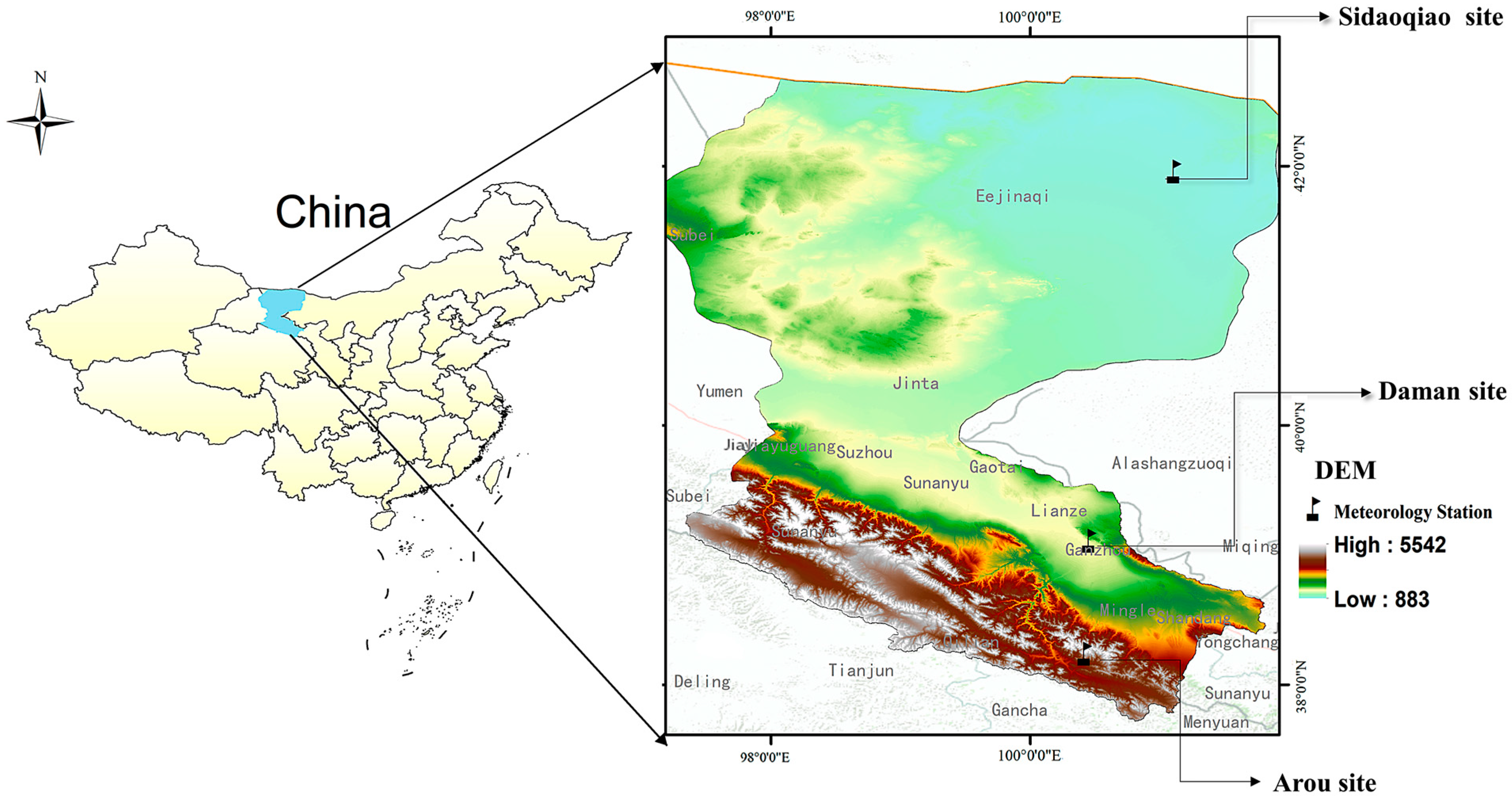
2.1. Study Area

The HRB (97°E–102°E, 38°N–43°N) is located in Northwest China, covering an area of approximately 142,900 km². The climate of the basin is influenced by the mid-to-high latitude westerly circulation and polar cold air masses [23]. From upstream to midstream and downstream, the basin exhibits a diverse natural landscape linked by water, including “ice/snow and permafrost—forests—meadows—artificial/natural oases—deserts—lakes” among other characteristics [24]. This region has characteristics of both cold and arid zones, with significant surface heterogeneity, especially the extreme aridity in the mountain cryosphere and the river delta regions, presenting a stark contrast, making it highly representative of climate research in Northwest China [25,26].

In this complex environment, accurately obtaining ET data within the basin is crucial for deeply understanding the regional water cycle and the energy exchange between land and atmosphere. Notably, another important reason for choosing the HRB as the study area is that previous researchers have conducted a series of long-term ecohydrological experiments here, and they have established a rich comprehensive observation network [27,28,29]. At its peak, the observation network included three superstations and twenty regular stations [30], accumulating a wealth of hydro-meteorological observation data [31], which lays a solid foundation for the research. This paper uses data from three superstations located in the upstream, midstream, and downstream, respectively. The distribution and information of the stations are shown in Figure 1 and

Table 1. Specific information on the three super-observatories upstream, in the middle, and downstream of the HRB.

Site Name	Longitude/°E	Latitude/°N	DEM/m	Site Location	Landscape
Arou	100.46	38.05	3033	Upstream	Subalpine meadow
Daman	100.37	38.86	1556	Midstream	Maize
Sidaoqiao	101.14	42.00	873	Downstream	Tamarix

.

2.2. Data Sources

In this paper, with four multi-source ET data products, including MOD16A2, HiTLL, SoGAE, and ETMonitor, after completing the adaptation study at the image scale and trend surface scale, the spatial and temporal characteristics of ET in the HRB were analyzed for the 10-year period of 2010–2019. Based on HRB subsurface characteristics and previous factor analyses of the effects of ET products [32], we comprehensively selected land use, elevation, slope, slope direction, vegetation index, temperature, and precipitation as the factors affecting ET, and analyzed the contribution value of their influence factors.

2.2.1. RS_ET Data

The site observation ET dataset is available from the National Tibetan Plateau Data Center (https://data.tpdc.ac.cn/, accessed on 11 May 2023) [33]. Based on the Penman–Monteith equation MOD16 data (MOD16A2) from the Internet (https://search.earthdata.nasa.gov/, accessed on 11 May 2023). It is based on the fusion of moderate resolution imaging spectroradiometer (MODIS) data with surface parameters used after analysis of Landsat Enhanced Thematic Mapping Plus (ETM+) data to drive the revised Surface Energy Balance System (SEBS) model. The High-Temporal and Landsat-Like surface ET in the HRB (2010–2016) (HiTLL) dataset and Multi-process parameterized ensemble model using biophysical and hydrological parameters/variables retrieved from satellite observations the ETMonitor dataset are available from the National Tibetan Plateau Data Center (https://data.tpdc.ac.cn/, accessed on 11 May 2023). The synthesis of actual ET global products is from the GEE platform based on in situ pixel evaluations of 12 global evapotranspiration products for different time periods, surface types, and conditions using high-quality flux eddy covariance (EC) to select high-performance products with global coverage (https://elnashar.users.earthengine.app/view/synthesizedet, accessed on 11 May 2023). See

Table 2. Specific characteristics of the coarse RS_ET products used in this study.

Product Category	ET Products	Temporal Extent	Spatial Coverage	Spatial Resolution	Temporal Resolution
Based on surface energy balance modeling	HiTLL ET V1.0 [22]	2010–2016	HRB	100 m	Daily
Based on Penman– Monteith model	MOD16A2 [34]	2000–2021	Global scale	1 km	8 days
Combinatorial models based on multi-process parameterization	ETMonitor [35]	2000–2019	Global scale	1 km	Daily
Synthetic evaporation products based on different data sources	Synthesis of global actual evapotranspiration [36]	1982–2019	Global scale	1 km	Monthly

for specific information on adopted products.

2.2.2. Satellite Data

This study utilizes the China Land Cover Dataset (CLCD) for reference land use data, which is derived from 300,000 Landsat images and validated with 5463 independent reference samples, achieving an overall product accuracy of 79.31% [37]. The CLCD dataset, with a spatial resolution of 30 m, captures the rapid urbanization and ecological projects in China, highlighting the impact of human activities on regional land cover under climate change. For this study, we selected the time series data from 2010 to 2019, including nine types of land use data. In this study, these nine types of land use data were reclassified into six categories: cropland, forest land, grassland, watersheds, unused land, and impervious surfaces, and land use dynamics and transfer analyses were conducted.

2.2.3. Terrain Data

The terrain data in this paper were obtained from the Digital elevation model of China (1 km) dataset from the spatiotemporal tripolar environmental big data platform (https://poles.tpdc.ac.cn/zh-hans/, accessed on 11 May 2023) [38]. To study the influence of terrain factors on ET in the HRB, according to the topographic characteristics of the watershed, we conducted a study of HRB elevation, slope, and slope direction data. We reclassified the elevation, slope, and direction data according to the topographic characteristics of the catchment.

2.2.4. Other Data

Precipitation data were obtained from the CHIRPS Daily: Climate Hazards Group InfraRed Precipitation With Station Data (Version 2.0 Final) dataset (https://developers.google.com/earth-engine/datasets, accessed on 11 May 2023), which combines 0.05° resolution satellite imagery with in situ station data to produce gridded precipitation time series for trend analysis and seasonal drought monitoring, and the data come together in a quasi-global precipitation dataset of more than 30 years [39]. The temperature dataset was obtained from the National Tibetan Plateau Data Center (https://data.tpdc.ac.cn/, accessed on 11 May 2023), and the resolution of the dataset is 1 km monthly (1901–2022) [40]. The normalized difference vegetation index (NDVI) dataset was obtained from the National Tibetan Plateau Data Center (https://cstr.cn/18406.11.Terre.tpdc.300330, accessed on 11 May 2023), and the resolution is 250 m monthly (2000–2022) [41].

2.3. Methods

2.3.1. Trend Analysis Methods

The Sen + Mann–Kendall method is a new approach to studying long-term trends in vegetation. Its advantage is that it does not require the samples to follow a specific distribution and is not disturbed by outliers [42,43].

$$\beta =M\mathrm{edian}\left({\displaystyle \frac{x_j-x_i}{j-i}}\right),\forall j>i$$

(1)

where $\beta$ is the trend of vegetation change, and $i$ and $j$ are the time sequence numbers representing the ET values at time $i$ and $j$, respectively. $\beta >0$ indicates an upward trend in vegetation cover, and $\beta <0$ indicates a downward trend in vegetation cover.

$$U_{MK}={\displaystyle \frac{\tau }{\left[Var{\left(\tau \right)}^{\frac{1}{2}}\right]}}$$

(2)

$$\mathrm{where}:\tau ={\sum }_{\begin{array}{c}i=1\end{array}}^{n-1}{\sum }_{\begin{array}{c}j=i+1\end{array}}\mathrm{sgn}\left(x_j-x_i\right);\mathrm{sgn}\left(\theta \right)=\left\{\begin{array}{c}1,if\theta >0\\ 0,if\theta =0\\ -1,if\theta <0\end{array}\right.$$

(3)

$$Var(\tau )={\displaystyle \frac{n(n-1)(2n+5)-\sum _{\begin{array}{c}t-1\end{array}}^m{t}_i(t_i-1)(2t_i-5)}{18}}$$

(4)

where $n$ is the number of series data, m is the number of concurrent (repeated dataset) values, and $t_i$ the number of ties for the $i^{th}$. The $U_{MK}$ converges to the standard normal distribution when $n>10$. The original assumption is that the series has no trend, and the bilateral trend test is used at a given level of significance α, to find the critical value $U_{\alpha /2}$ in the normal distribution table. When $\left|U_{MK}\right|<U_{\alpha /2}$, the original hypothesis is accepted, meaning that the trend is not significant; if $\left|U_{MK}\right|>U_{\alpha /2}$, the original assumption is rejected, that is, the trend is significant.

According to Wang et al.’s study [44,45], the ET trend level criterion was defined as 4 levels, namely significant increase ($\beta >0$, passes the 0.05 test); slight increase ($\beta >0$, fails the 0.05 test); significant decrease ($\beta <0$, passes the 0.05 test); slight decrease ($\beta <0$, fails the 0.05 test).

2.3.2. Calculation of Mean ET Values

We used the Mean Centre tool of ArcGIS 10.8 to create a new class of point elements, where each element represents a mean center that is determined element by element based on the average of the input values. The main formula for this is shown in Equation (5):

$$\overline{X}={\displaystyle \frac{1}{n}}{\sum }_{i=1}^n{x}_i,\overline{y}={\displaystyle \frac{1}{n}}{\sum }_{i=1}^n{y}_i$$

(5)

where $x_i$ denotes X-axis coordinates and $y_i$ denotes Y-axis coordinates, $i$ = 1, 2, ..., n. We used this method to calculate the 10-year average ET and seasonal average ET in the study area.

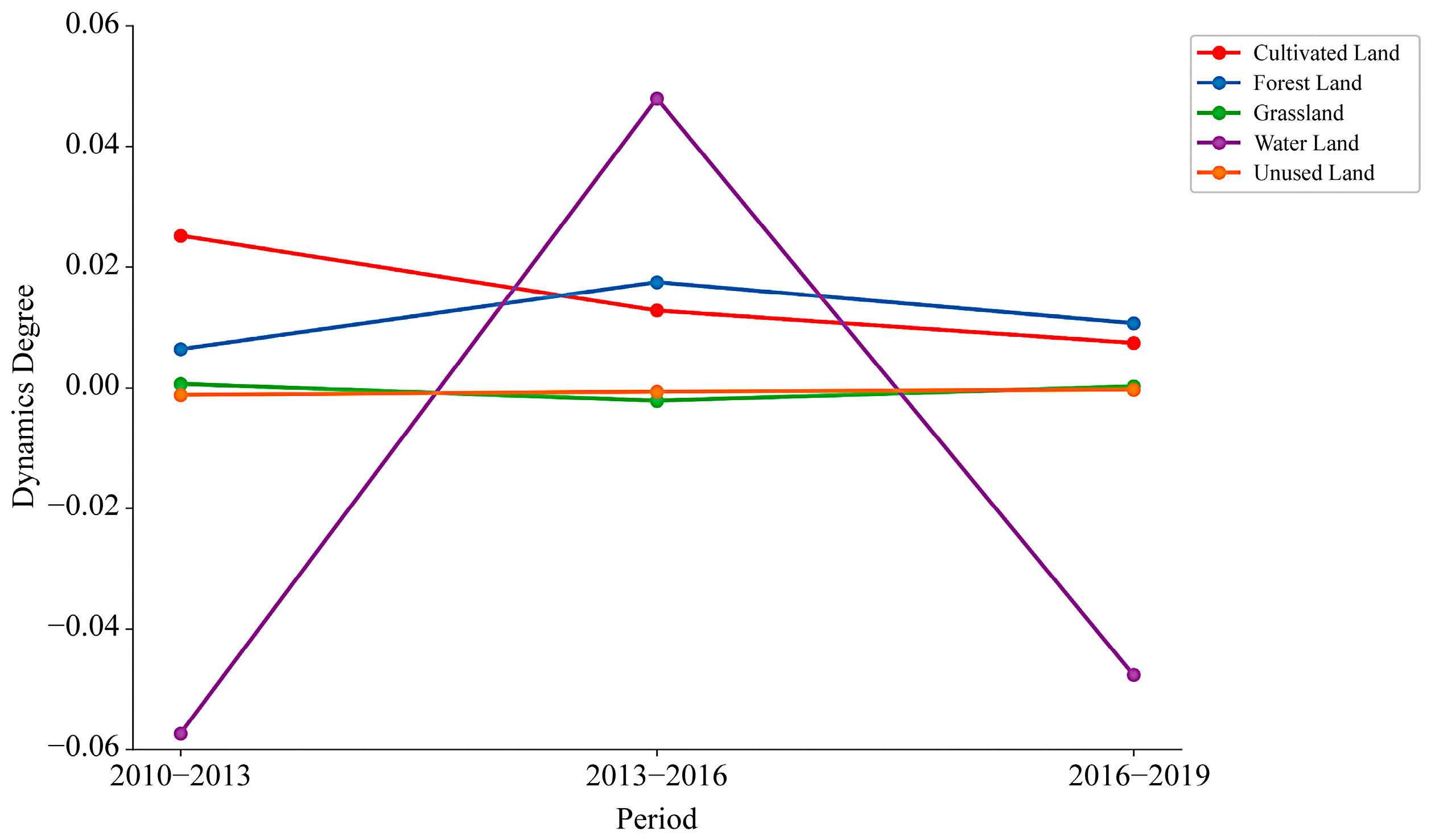
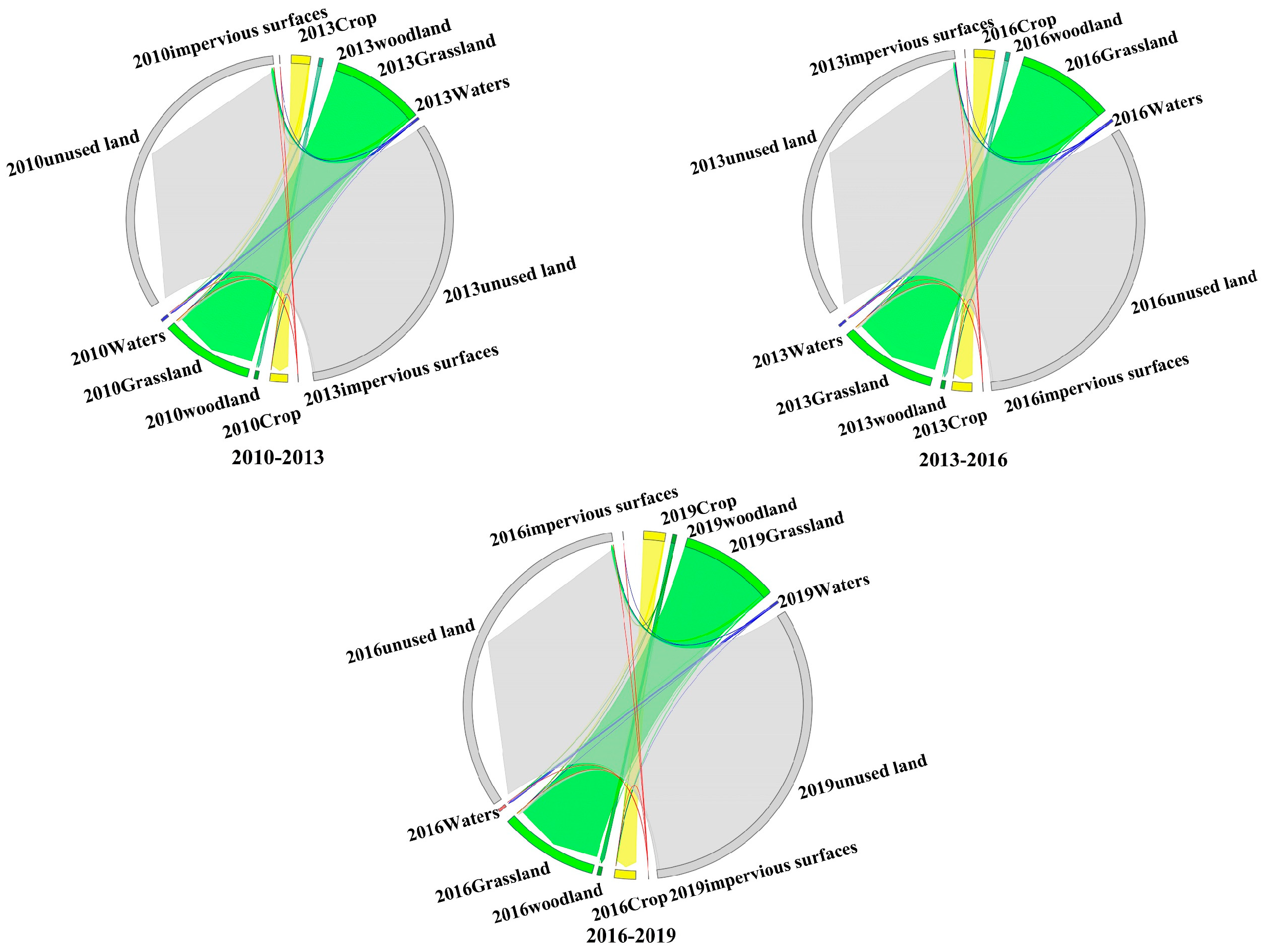
2.3.3. Analysis of Land Use Dynamic

Land use dynamic is a visual reflection of the speed of change in land use types, divided into single dynamic degree R and comprehensive dynamic degree LC. The land use single dynamic degree can quantitatively describe the speed of regional land use change, and it plays an important role in comparing the regional differences in land use change and predicting future land use trends [46]. The comprehensive dynamic degree refers to the overall indicator derived after considering the change situation of many different types of land use, which is used to describe the overall change of land use structure in a region or country in a certain period. The change situation is an overall indicator derived from the comprehensive consideration of many different types of land use, which is used to describe the overall change in land use structure of a region or a country in a certain period [47,48]. It can reflect the development and utilization of land resources, changes in the ecological environment, and the trend of sustainable development [49]. The calculation formulas are shown as follows:

(1)

Relative rate of change for a single land use type:

$$R={\displaystyle \frac{\left|K_b-K_a\right|C_a}{K_a\left|C_b-C_a\right|}}$$

(6)

where $K_a$ and $K_b$ denote the area of a particular land use type within the HRB at the beginning and end of the study period, respectively; $C_a$ and $C_b$ denote the area of the study area at the beginning and end of the study period, respectively. By calculating this index, it is possible to describe the changes in that particular land-use type over the study period and thus assess the dynamics of land resource use.

(2)

Integration of land use dynamics:

The equation for quantitative changes in land use types:

$$K={\displaystyle \frac{U_b-U_a}{U_a}}\cdot {\displaystyle \frac{1}{T}}\cdot 100\mathrm{\%}$$

(7)

where $U_a$ is the amount of a land use type at the start of the study, $U_b$ is the amount of that land use type at the end of the study period, and $T$ is the length of the study. If $T$ is set to years, the value of $K$ is the annual rate of change of that land use type during the study period.

$$L_C={\displaystyle \frac{\sum _{i=1}^n\mathsf{\Delta }{L}_{U_{i-j}}}{2\sum _{i=1}^n{L}_{Ui}}}{\displaystyle \frac{1}{T}}\times 100\mathrm{\%}$$

(8)

where $L_{U_i}$ is the area of land use type $i$ at the start time of monitoring, $\mathsf{\Delta }{L}_{U_{i-i}}$ is the absolute value of the area of land use type $i$ converted to non- $i$ land use type during the monitoring period, and $T$ is the length of the monitoring period. When $T$ is set to years, the value of $L_C$ represents the annual rate of change in land use in the study area. This index can be used to describe the rate of change in regional land use and help assess the utilization of land resources and trends in the HRB.

2.3.4. Land Use Transfer Matrix Analysis

By using the land use transfer matrix to describe the conversion relationship between land use types in different periods in the study area, it is possible to depict the changing characteristics of the land use structure and the direction of mutual transfer, thus reflecting the trend of the transfer of land use types [50,51]. In this study, the land use matrices for 2010–2013, 2013–2016, and 2016–2019 were obtained using superposition analysis and statistical tools to analyze the spatial and temporal changes in land use in the HRB over the last 10 years. The formulas are as follows:

$$S_{ij}=\left[\begin{array}{ccc}{S}_{11}& S_{12}& \cdots S_{1g}\\ S_{21}& S_{22}& \cdots S_{2g}\\ ⋮& ⋮& ⋮\\ S_{k1}& S_{k2}& \cdots S_{ka}\end{array}\right]$$

(9)

where $S_{ij}$ represents the land use status, and $k$ and $g$ are different land use types.

2.3.5. Optimal Parameter-Based Geoprobe Model

The Optimal Parameters-based Geographical Detector model (OPGD) is a tool for detecting and revealing spatial differences between data [52]. In this model, the discrepancy factor is measured by $Q$. The Q value of the number of each type X (dependent variable) in the probes represents the significance of the factor. q takes the value in the range [0, 1], where a larger Q value indicates that the influencing factor is stronger in explaining the target variable (e.g., ET), and a smaller Q value indicates that the influencing factor is weaker in explaining the target variable [53]. The Q value is calculated by the following formula:

$$Q=1-{\displaystyle \frac{\sum _{j=1}^i{H}_j{\sigma }_j^2}{H{\sigma }^2}}$$

(10)

where $Q$ denotes the differentiation factor; $i$ denotes the number of categories of the variable; $j$ denotes the specific type; $H_j$ denotes the number of units; and ${\sigma }_j$ denotes the variance.

In this paper, we use the interaction detection function of OPGD to analyze the interaction between different image factors, which is realized by Geodetector software (http://geodetector.cn/index.html). To ensure the consistency of the Geodetector input data, we used the natural breakpoint method in the reclassification tool to classify the different influencing factors of ET in the HRB. These factors were classified into six categories, namely temperature, DEM, NDVI, precipitation, slope, land use, and slope direction based on the main criteria of each factor, and were analyzed in the OPGD model [54]. By analyzing and calculating the data, it is possible to determine which factors have a greater influence on ET in the HRB, thus helping to reveal the spatial differences between different influencing factors. Using the OPGD model, the relationship between ET and different influencing factors can be better understood and the degree of influence of the influencing factors can be found [55], which can provide an important reference for further research and decision-making on, for example, water resource utilization in the HRB.

3. Results

3.1. Multiple Products Adaptability Analysis in the HRB

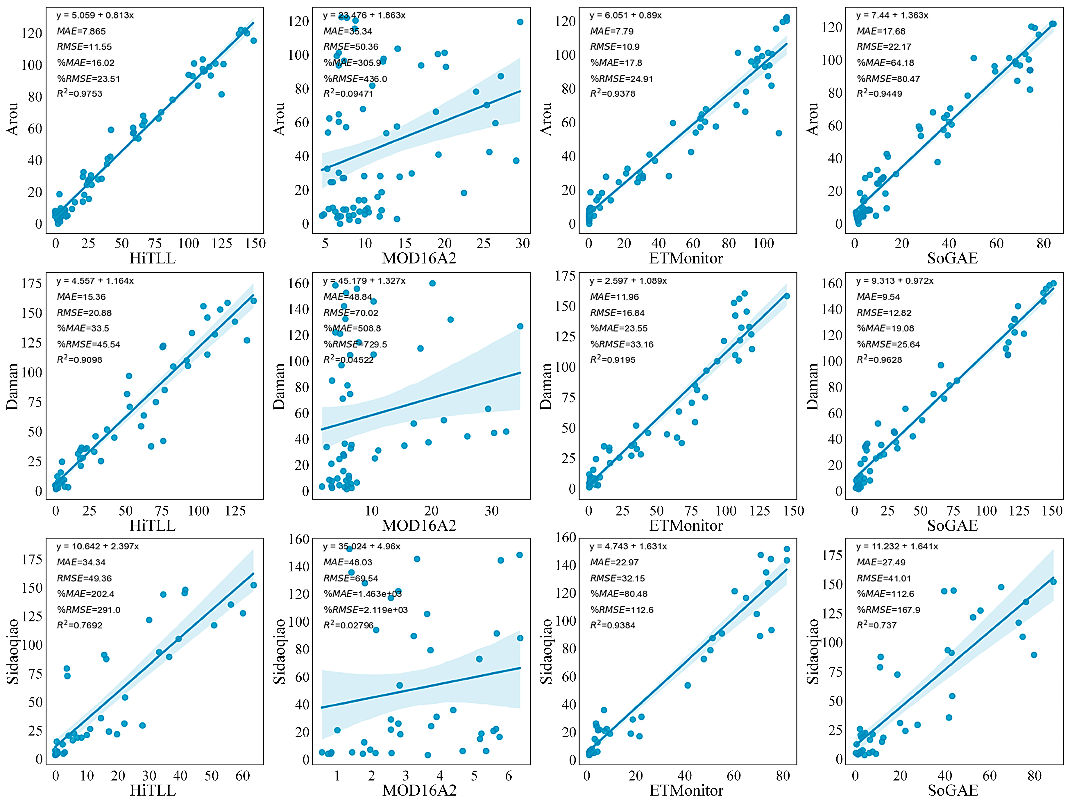
3.1.1. Study of Applicability Based on Site Scale

At the site scale, we conducted a linear regression analysis of four RS_ET products—HiTLL, MOD16A2, ETMonitor, and SoGAE—at the site scale in three superstation sites in the upstream, midstream, and downstream in the HRB.

It is evident from Figure 2 that there is a positive linear relationship between product ET estimates and ground truth measurements for all variables. In the HRB, HiTLL demonstrated optimal performance at the Arou superstation site with an R² (RMSE) of 0.9753 (11.55), but it showed a significant decline at the Sidaoqiao superstation with an R² (RMSE) of 0.7692 (49.36), indicating its sensitivity to different environmental conditions. Although it performed excellently at certain sites, this variability could affect its consistency and credibility as a basin-scale research tool. The MOD16A2 product showed a noticeable decline in performance compared to other products at all sites, suggesting some deficiencies in underlying surface data processing in the HRB, and significant data gaps in the midstream and downstream regions; thus, for HRB, the MOD16A2 product is not highly applicable. The SoGAE product had the highest R² (0.9628) and the lower RMSE (12.82) at the Daman superstation site, indicating high concurrence between the synthesis estimates and actual data at this site. However, its R² (RMSE) value is 0.7337 (41.01) at the Sidaoqiao site, showing some instability. In contrast, ETMonitoor showed significant advantages, with R² (RMSE) values of 0.9378 (10.9) and 0.9384 (16.84) at the Arou superstation and Daman superstation, respectively, and a high (low) R² (RMSE) value of 0.9195 (32.15) at the Sidaoqiao superstation, indicating that ETMonitor provides relatively stable and reliable ET estimates at all sites in the HRB, essential for basin-scale research. Although the R² value at the Sidaoqiao site was slightly lower than at other sites, ETMonitor’s overall performance demonstrated its suitability as a comprehensive monitoring tool.

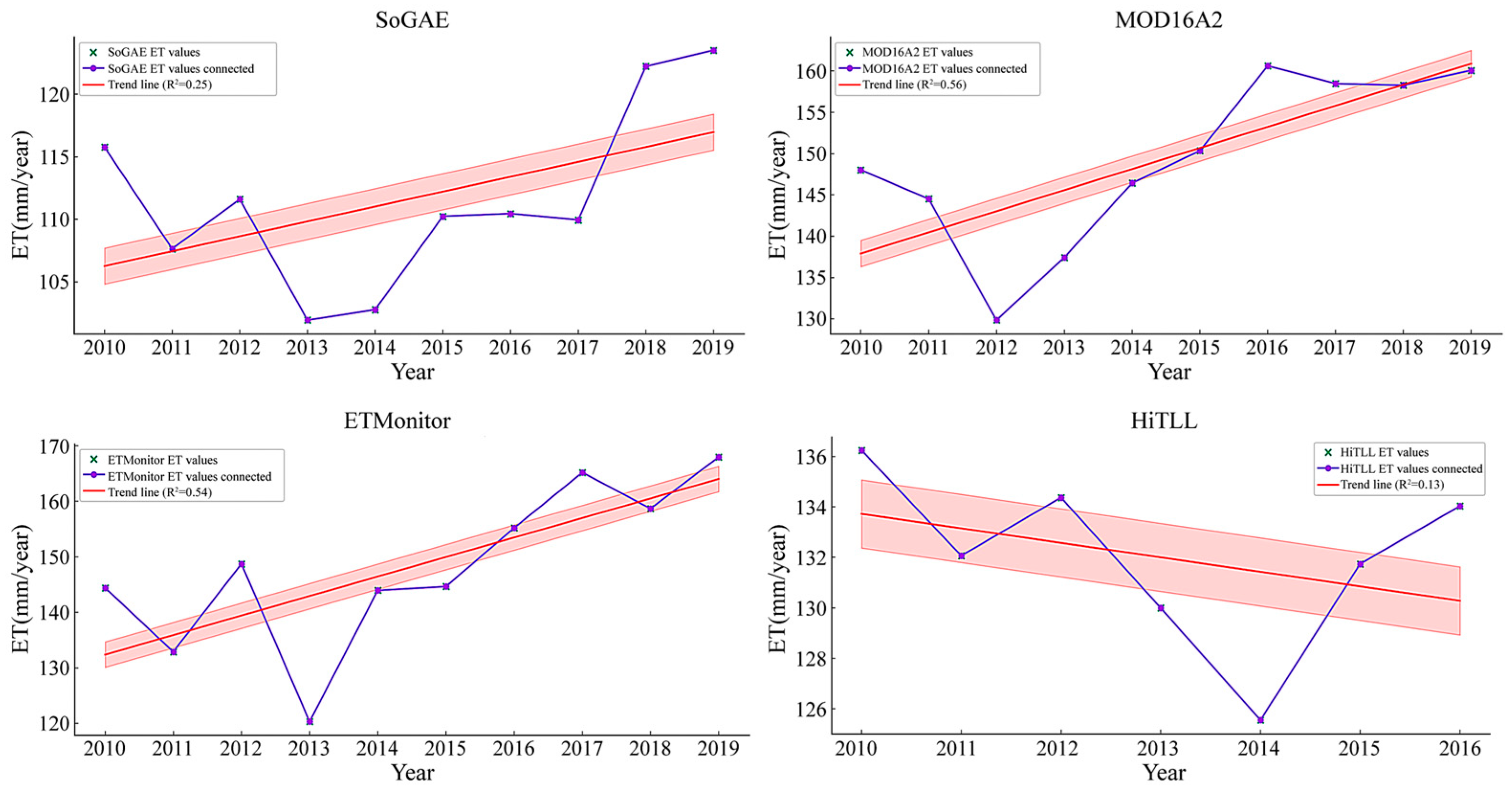
3.1.2. Trend Study of RS_ET Products

According to Figure 3, the R² of the trend line for SoGAE over multiple years is 0.25, indicating a weak correlation between ET values and time. The overall trend seems to be slightly increasing. The R² of the trend line for MOD16A2 is 0.56, indicating a moderate fit. The ET values show an overall increasing trend over time. The ETMonitor trend line has an R² value of 0.54, similar to MOD16A2, indicating a moderate fit. The ET values also showed a general upward trend over the years. The trendline R² value of 0.13 for HiTLL, on the other hand, is relatively low, which may be due to its shorter time series and the poor fit of its ET values to the trendline. The data show a high degree of variability, and the explanation of trend changes is not clear. In conclusion, the ETMonitor and MOD16A2 products seem to provide more consistent and better-fitting trends compared to other products.

This rising trend in ET may have significant implications for water resource management and agricultural planning in the basin, especially given the arid climate of the basin and the importance of water in sustaining agriculture and ecosystems in the region [56]. At the same time, ET emphasizes the need for continuous monitoring and adaptive water management strategies to ensure the sustainability of HRB water resources under changing environmental conditions.

To further select a product that is more suitable for the basin-wide scale of HRB, we analyzed the trends of the different products over the years, and the results are shown in Figure 4. In comparing the four products, we found that each of them has its characteristics in terms of spatial distribution, which may be related to their algorithms, resolution, accuracy of input data, and the degree of calibration in a particular area. The SoGAE shows significant degradation over large areas, which may make it more sensitive to specific applications such as degraded area studies, but less capable of basin-wide interpretation. The HiTLL shows moderate improvement and degradation but overall has fewer improved contours than the ETMonitor. The MOD16A2 shows significant degradation over large areas, which may indicate that it is less applicable in the HRB, has a serious lack of numerical power, and has substantial data missing in the middle and lower reaches. On the other hand, the ETMonitor seems to provide a relatively balanced assessment with both improved and degraded areas, suggesting that its estimates are less variable and may be more suitable for watershed-scale studies. Considering the performance of ETMonitor in terms of spatial distribution and its relatively balanced areas of improvement and degradation, it may be a more appropriate choice for evaluating ET across the HRB watershed.

Overall, the results from the different products show different ET trends, which may be due to the different algorithms, input data, and calibration methods used for each ET estimation product. However, ETMonitor appears to be suitable for a basin-wide study at the HRB in terms of several considerations, including trend interpretation capabilities and data completeness. The upward trend in ET could have significant implications for water management and agricultural planning in the basin, especially given the arid climate of the region and the importance of water resources in sustaining the region’s agriculture and ecosystems. There is a need to emphasize continuous monitoring and adaptive water management strategies to ensure the sustainability of water resources in the HRB under changing environmental conditions.

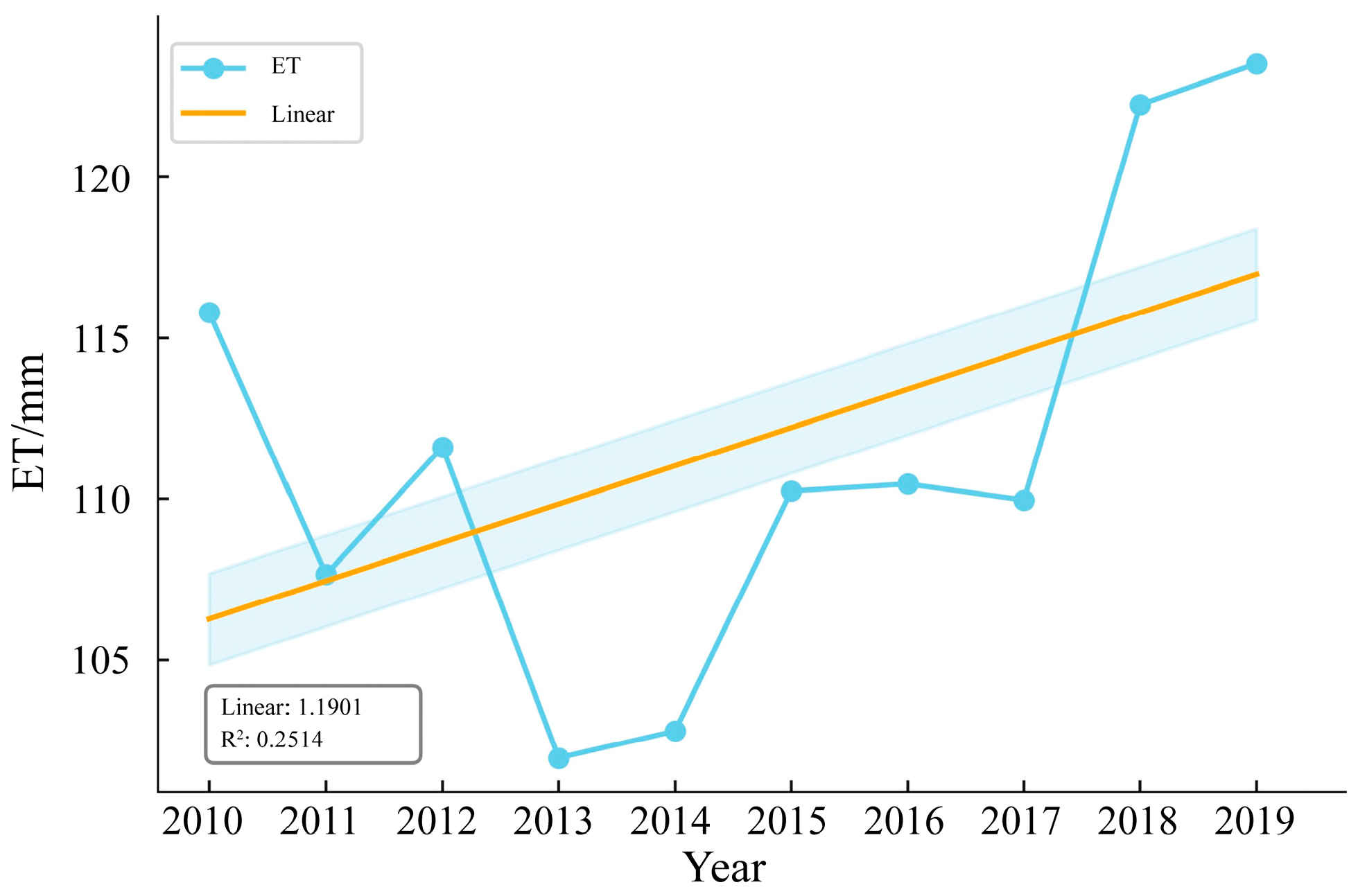
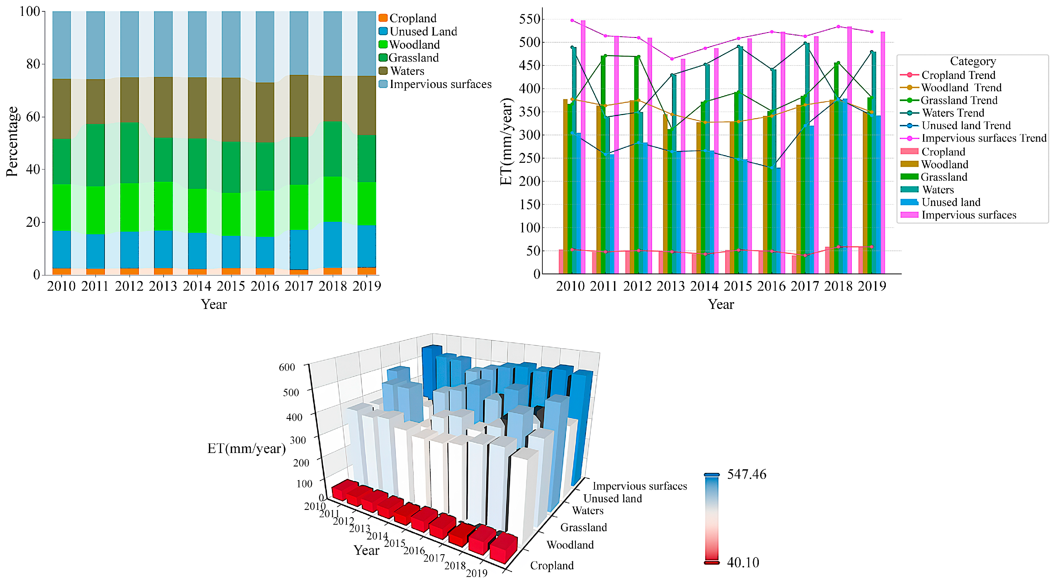
3.2. Characteristics of ET Changes

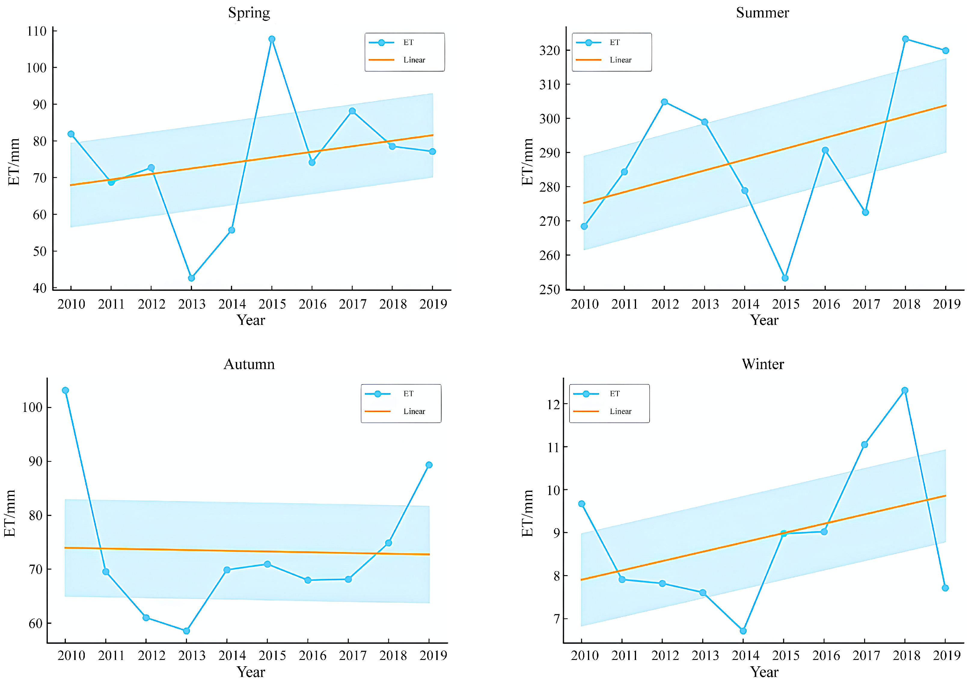
3.2.1. Seasonal and Interannual Variability in ET

From 2010 to 2019, the annual average ET in the HRB, as shown in Figure 5, shows that, over the past 20 years, the overall trend of increasing ET in the entire basin is fluctuating. The ET in the HRB showed an increasing trend year by year from 2010 to 2019. The slope of the linear trend line is approximately 1.1901, indicating an average annual increase of 1.1901 mm in ET. The yearly changes in ET in the HRB are as follows: 2011 decreased by 8.14 mm compared to 2010; 2012 increased by 3.96 mm compared to 2011; 2013 decreased by 9.66 mm compared to 2012; 2014 increased by 0.84 mm compared to 2013; 2015 increased by 7.45 mm compared to 2014; 2016 increased by 0.22 mm compared to 2015; 2017 decreased by 0.50 mm compared to 2016; 2018 increased by 12.28 mm compared to 2017; 2019 increased by 1.27 mm compared to 2018.

We can observe that the annual variations in ET are not unidirectional; they exhibit a pattern of increases and decreases. These variations may be influenced by multiple factors, including climate change, interannual fluctuations in precipitation patterns, and changes in surface vegetation cover. This variability further emphasizes the importance of considering multiple variables when predicting ET.

To better understand the intra-annual variability in ET in the HRB, the mean value method was used to determine the ET values for different seasons, as shown in Figure 6. Our analysis reveals that the ET exhibits distinct seasonal variations in the HRB. The highest ET occurs in summer, which aligns with the higher temperatures and possibly abundant sunlight during this season, factors that increase water evaporation and plant transpiration. Winter has the lowest ET values, likely due to lower temperatures, slow vegetation growth, and shorter daylight hours reducing water evaporation.

Spring and autumn ET values are in the medium range, with relatively less variability. However, spring shows slightly more variability than autumn, possibly influenced by spring precipitation and the activity of vegetation growth. The trend line shows that, despite obvious seasonal fluctuations, the long-term trend indicates that the ET in summer and winter is increasing, while spring shows a slight downward trend and autumn remains relatively stable. These seasonal changes are likely related to long-term climate patterns, changes in land use, and regional water management policies.

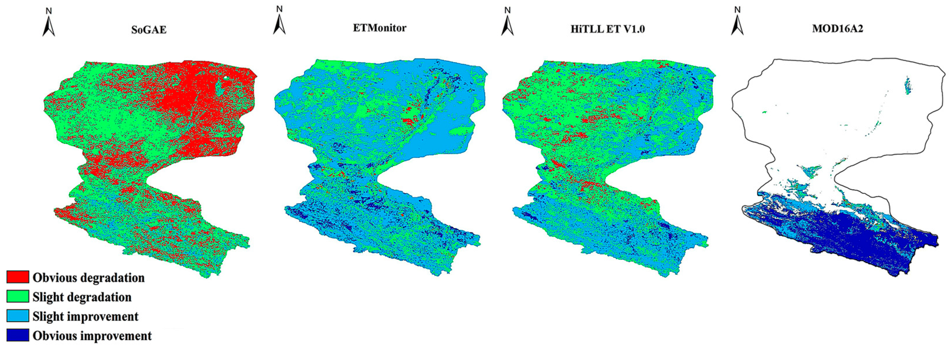
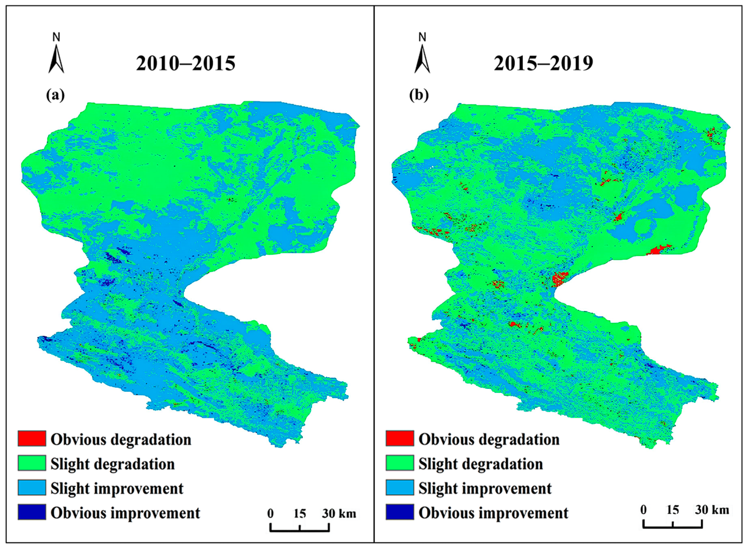
3.2.2. Analysis of Spatial and Temporal Variations of ET

The spatial distribution of the annual average ET over the past 10 years in the HRB is shown in Figure 7a. The multi-year average ET in HRB ranges between 1811.91 and 23.46 mm/year. According to Figure 7a, the upstream areas of the HRB generally have higher ET values, while downstream values are lower. It can be seen from the figure that the ET in the upstream areas of the HRB is significantly higher than that in the downstream areas (as seen in the upper part of the image). The blue areas upstream may represent rivers, lakes, or irrigated areas, while the high values in the upstream areas may be related to sparse vegetation or arid climatic conditions. This distribution pattern is significant for understanding the cycle and management of water resources within the basin.

To further observe the spatial trends of ET changes from 2000 to 2019, we used the Sen + Mann–Kendall trend test method, dividing the ET change interval by the natural break method, obtaining the spatial distribution of the interannual linear trends in HRB over the past 10 years, as shown in Figure 7b. Figure 7b displays the trend map of ET changes in the HRB from 2010 to 2019. With different color markings, we can see that, during this period, the basin shows clear areas of significant land degradation (red areas) and minor degradation (orange areas), which may have suffered from drought, overuse, or other environmental stresses, leading to reduced vegetation and thereby increased ET. The areas shown in light and dark blue indicate improvements in land conditions, possibly due to vegetation recovery or effective water resource management, reflecting a reduction in ET, suggesting more effective water conservation in these areas. The midstream areas show significant signs of degradation, appearing as red spots, indicating a significant increase in ET values over the decade, likely due to reduced vegetation or overuse of water resources.

Meanwhile, the extensive blue and light blue areas indicate that, in other parts of the basin, the ET values have decreased over these ten years, which may imply good conditions for water retention or vegetation recovery, reflecting an overall improvement in ecological conditions. These trends provide important geographical information for assessing environmental management and planning in the HRB. To further study the spatial changes in ET in the HRB over the past 10 years, ET data from 2010 to 2019 were superimposed, and the Sen + Mann–Kendall method was used to calculate the spatial distribution pattern and its evolutionary characteristics, as shown in Figure 8. From 2010 to 2014, the ET in the upstream and downstream of the HRB showed a slight increasing trend, accounting for about 58.41% of the total basin area, while the main trend in the midstream was a gradual weakening, accounting for about 37.21% of the total basin area. In addition, some points showed significant increases and decreases, accounting for 1.35% and 3.03%, respectively.

During 2015–2019, the downstream part of the HRB generally showed a slight increase in ET, accounting for about 51.09% of the total basin area, while the upstream and midstream parts mainly showed a gradual weakening, accounting for about 44.56% of the total basin area. In addition, between 2015 and 2019, only a very small part of ET in the HRB showed a significant increase, accounting for about 0.20% of the total area, while the significantly decreasing parts accounted for about 4.15%.

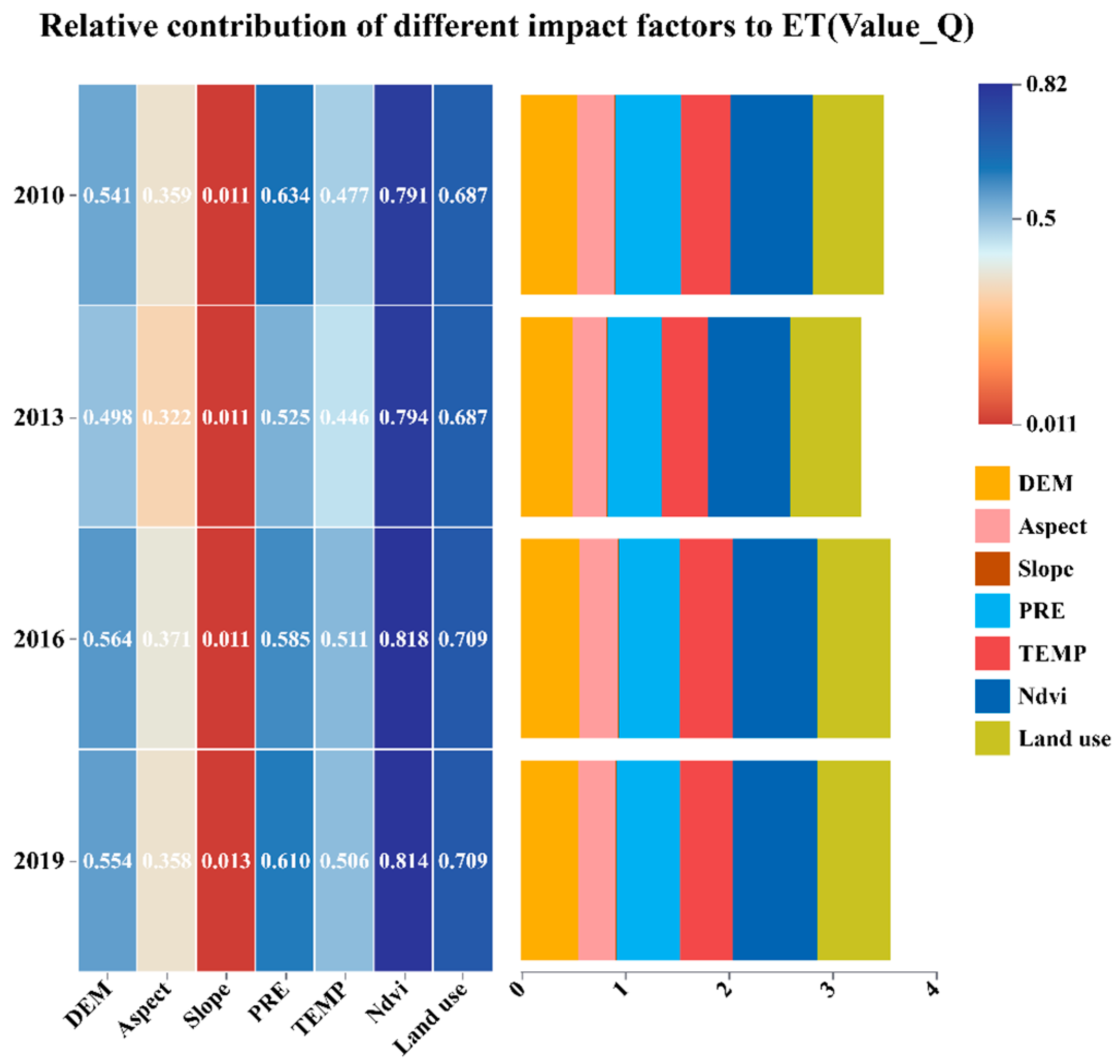
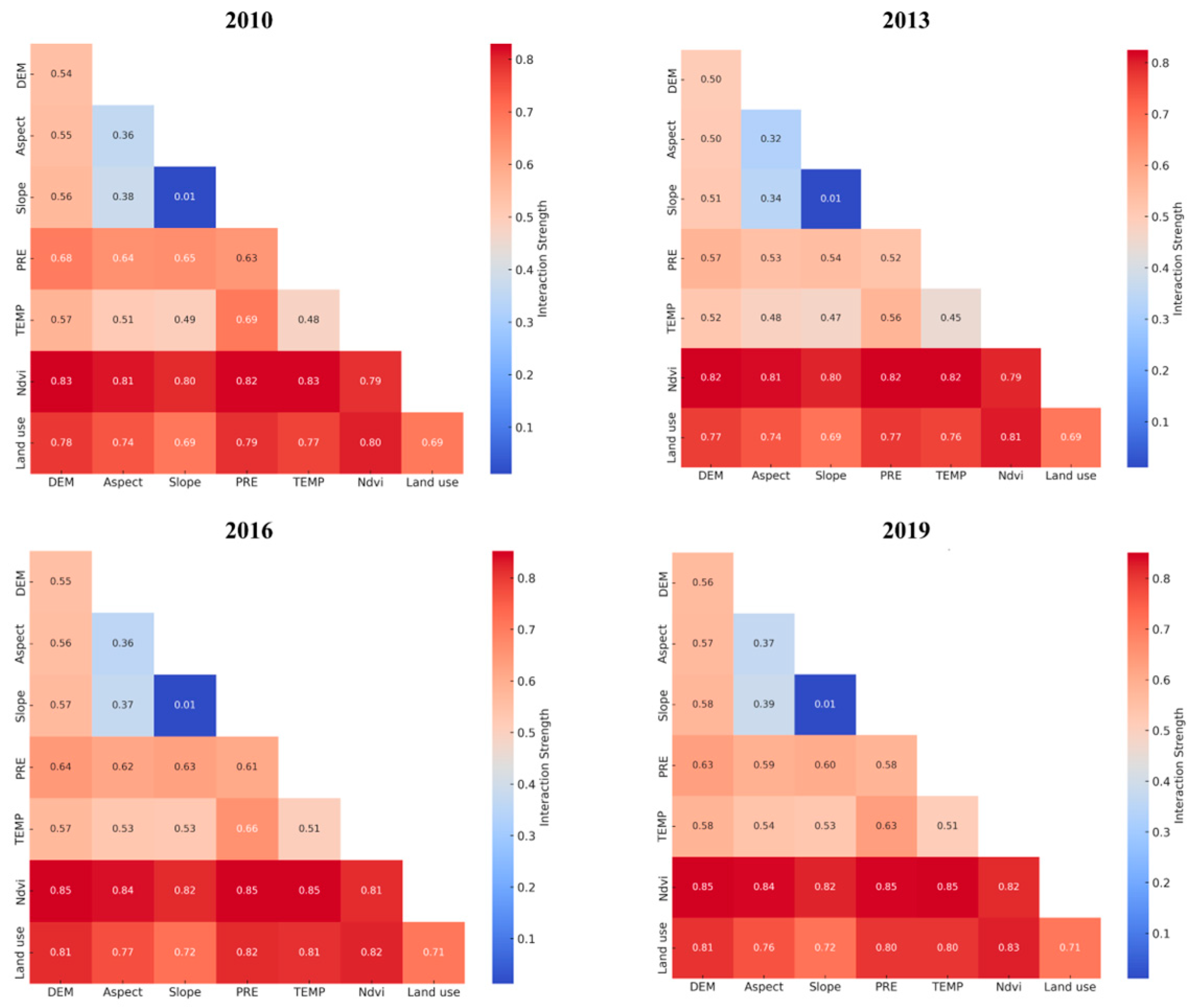
3.3. Analysis of ET Impact Factors

3.3.1. Analysis of Land Use Impact Factors

As shown in Figure 9 and

Table 3. Trend map of land use dynamics in the HRB (2010–2019).

		2010–2013	2013–2016	2016–2019
	Cropland	2.52%	1.28%	0.74%
	Woodland	0.64%	1.75%	1.07%
Single dynamics	Grassland	0.06%	−0.22%	0.02%
	Water	−5.74%	4.80%	−4.76%
	Unutilized land	4.08%	2.79%	7.48%
	Impervious surface	4.08%	2.79%	7.48%
Comprehensive dynamics		0.12%	0.10%	0.05%

, we calculated the single dynamic degree for each type of land use in the HRB and the comprehensive dynamic degree for the entire basin. We identified the complexity of land use changes within the HRB and their temporal characteristics.

During the observation period, the single dynamic degree of cropland showed a decreasing trend, from 2.52% in 2010–2013 to 0.74 in 2016–2019, indicating a slowdown in the rate of cropland conversion throughout the observation period, but still showing some changes. The single dynamic degree of forest land showed a fluctuating increase throughout the study period, from 0.64% in 2010–2013 to 1.07% in 2016–2019, reflecting active changes in the increase or decrease in forest area, and also indicating an increase in ecological conservation activities in the HRB. The single dynamic degree of grassland changed little, with a small range of fluctuation throughout the study period, but there was a slight negative growth from 2013 to 2016, indicating a slight reduction in grassland area during these periods.

The comprehensive dynamic degree indicates that the overall speed of land use change in the HRB is relatively slow, but there are still subtle changes. This result suggests that, although changes in individual land use types may be significant, the overall stability of land use is high, with limited variability.

The dynamic changes in land use data of the study area in different years are shown in Figure 10 and Figure 11. Between 2010 and 2013, we observed significant land cover changes mainly characterized by a slight decrease in cropland, which decreased by approximately 56,975 ha, primarily converting to grassland (10,469 ha) and forest land (35 ha); concurrently, the areas of forest and grassland showed an increasing trend, with forest land increasing by 12,126 ha and grassland increasing by 28,947 ha. The area of water bodies also decreased during this period, decreasing by approximately 6427 ha, mainly converting to other categories such as cropland (532 ha) and unused land (19,334 ha). Finally, the area of unused land showed significant growth, increasing by approximately 10,433 ha. From 2013 to 2016, the total area of cropland increased by approximately 61,086 ha, mainly due to the conversion of grassland (24,515 ha) and unused land (12,533 ha) into cropland. The total area of forest land also expanded by approximately 12,441 ha, mainly due to the conversion of cropland (48 ha) into forest land. The total area of grassland steadily increased by approximately 28,962 ha, primarily from converted cropland. The total area of water bodies slightly decreased by approximately 6602 ha, with their areas mainly converting to cropland (331 ha) and unused land (2804 ha). Additionally, the area of unused land continued to expand by approximately 10,411 ha during this period. Between 2016 and 2019, the area of cropland continued to increase by approximately 63,056 ha, mainly due to the trend of converting grassland (31,787 ha) and unused land (7563 ha) into cropland; the area of forest land significantly increased by approximately 13,047 ha, mainly due to the conversion of grassland (5630 ha) into forest land; meanwhile, the area of grassland decreased by approximately 10,362 ha, mainly converting to cropland (31,787 ha) and unused land (68,338 ha); the area of water bodies significantly decreased by approximately 6322 ha, mainly converting to unused land (15,791 ha); nevertheless, the area of unused land still increased by approximately 10,389 ha during this period.

To further study the changes in ET characteristics of different land cover types in the HRB, we analyzed and statistically examined the interannual trends of ET for different land cover types from 2010 to 2019, as shown in Figure 12. The results reveal that data from 2010 to 2019 in the HRB showed different patterns of ET for different land cover types. Over this decade, the ET values for cropland fluctuated slightly but showed a slight upward trend, indicating a stable demand for water in agricultural production, possibly due to consistent farming techniques or crop types. The changes in forest and grassland were more pronounced, possibly due to natural factors affecting vegetation such as precipitation patterns, temperature, and human activities such as deforestation or reforestation. Notably, the peaks and troughs in grassland were most pronounced, suggesting that this land cover type may be most sensitive to annual climate variations.

The category of water bodies, which may include lakes and rivers, had the highest overall ET values, reflecting continuous evaporation associated with open water surfaces. These values peaked in the middle of the decade, suggesting increased temperatures or reduced precipitation during this period. Compared to vegetated areas, the interannual changes in unused land and impervious surfaces were less apparent. The trends across all land cover types in high-latitude areas highlighted the complex interactions between climate factors, land management measures, and the intrinsic characteristics of each land cover type affecting the dynamics of ET. The detailed trends in the charts show how each land cover type uniquely responds to environmental and anthropogenic factors over the years. Overall, this study provides important scientific evidence for understanding land use changes in the area and offers references for related land resource management and policy-making.

3.3.2. Correlation Analysis of Terrain Influence Factors

Elevation is a fundamental topographic feature that affects factors such as soil moisture and surface runoff in a watershed, thereby influencing changes in ET [57,58]. Based on this, after overlaying land use data with ET, we further analyzed the spatial overlay of land cover types within the HRB with elevation, slope, and aspect data, and calculated the average ET for each land cover type at different elevations, as shown in Figure 13.

When analyzing DEM-related charts, we found that the average ET of different land cover types showed different trends with increasing elevation. Generally, as elevation increases, temperature and vegetation decrease, leading to a decrease in ET values. In the charts, cropland and forest land show a decrease in ET with increasing elevation, indicating the potential effects of climate change and vegetation distribution. The ET of water bodies changes little, suggesting that their evaporation is mainly controlled by the characteristics of the water bodies themselves, rather than elevation.

In summary, by integrating the analysis results of the three aspects of topographic data, we can conclude that the ET of different land cover types is influenced by a combination of topographic factors such as elevation, slope, and aspect. Elevation mainly affects ET by influencing temperature and vegetation distribution, slope affects ET by changing the way water moves, and aspect changes ET by altering the amount of sunlight and wind the land receives. These analyses help us understand the hydrological processes of different land cover types within the watershed and provide a scientific basis for water resource management and land use planning.

3.3.3. Analysis of the Relative Contribution of Different Influencing Factors to ET

To gain a more specific understanding of the impact of different influencing factors on ET in the HRB, we conducted a geographical detector analysis of multiple influencing factors on ET in the HRB, as shown in Figure 14 and Figure 15. We noticed that, from 2010 to 2019, there were significant differences in the contributions of factors such as temperature (TEMP), vegetation index (NDVI), precipitation (PRE), and land use to ET. It is also noteworthy that, although some factor detectors had Q values of less than 0.5, indicating a lower explanatory power for ET, the interaction of different influencing factors achieved a synergistic effect; therefore, these influencing factors should not be overlooked.

In the analysis of the geographical detector results for ET in the HRB from 2010 to 2019 seen in Figure 14, at the same time, we added a standard scale to indicate the share of different ET impact factors. The vegetation index (NDVI) was consistently the most significant factor affecting ET, with its influence peaking in 2016 with a Q value of 0.818 and remaining above 0.7 in other years. Precipitation (PRE) and temperature (TEMP) were also significant influencing factors, with their relationship to ET showing some variability across different years, with temperature’s influence increasing in 2019 with a Q value of 0.506. Elevation (DEM), although varying slightly each year, maintained a relatively high overall contribution to ET, while the influence of slope was relatively minor, possibly reflecting the relatively stable impact of topography on the hydrological cycle.

The relative contribution of land use was higher in 2016 and 2019, with Q values of 0.709, indicating that land cover changes, especially those related to urbanization and agricultural activities, had an increasing impact on ET in those years. Over time, changes in land use methods may have an increasingly significant impact on ET, highlighting the importance of considering land planning and management policies in watershed resource management. These analysis results not only reveal the diversity of changes in ET but also emphasize the necessity of considering multiple factors, including vegetation and land use, in water resource management and ecological conservation strategies.

Through the analysis of Figure 15, we observed the dynamic changes in interactive factors for actual ET in the HRB from 2010 to 2019. Throughout this period, the interaction between the vegetation index (NDVI) and topography (DEM) consistently dominated. Specifically, in 2010 the interaction between NDVI and DEM had a Q value of 0.83, and in 2013 it was similarly high at 0.82, indicating that ET during those years was significantly influenced by the interplay of vegetation cover and elevation. By 2016, this interaction’s Q value even rose to 0.85, and the trend continued in 2019, demonstrating a strong synergistic effect between vegetation and topography on ET. Regarding land use, over time, this factor’s contribution to ET has significantly increased, with Q values of 0.83 in 2016 and 0.81 in 2019, reflecting that changes in land cover, especially changes caused by human activities, have an increasingly important impact on regional ET.

In integrating the heatmap data for these years, it is evident that NDVI’s consistently high values and its strong interactions with other environmental variables underscore the crucial role of vegetation health in water cycling and climate regulation. These patterns suggest that, in formulating water resource management and ecological conservation strategies, the interactions between vegetation cover and topographic variables must be fully considered. Moreover, it also highlights how land use decisions, including agricultural development and urban expansion, impact surface water evaporation and plant transpiration, thereby affecting the overall water balance of the watershed. These detailed insights provide significant scientific support for devising more effective watershed management strategies and measures to adapt to climate change.

4. Discussion

4.1. Adaptation of RS_ET Products

In the adaptability study of multi-source RS_ET products in the HRB, we comprehensively assessed the performance of ETMonitor, MOD16A2, HiTLL, and SoGAE on both site scale and trend surface scale. Using linear regression analysis, error metrics, and the slope of trend lines along with the Sen + Mann–Kendall method among other multivariate testing methods, we explored the adaptability and accuracy of each model across different scales in the HRB. We found that ETMonitor showed more stable and consistent performance across the entire basin.

On the site scale, ETMonitor showed high consistency and stability, particularly at the Arou and Daman superstations, where R² values exceeded 0.93. This indicates that ETMonitor can provide reliable ET estimates in different underlying surface environments in the upper, middle, and lower reaches of HRB. In contrast, HiTLL, although performing best at the Arou site (R² = 0.9753, RMSE = 11.55), showed a significant performance decline at the Sidaoqiao site (R² = 0.7692, RMSE = 49.36), indicating large fluctuations in numerical estimation performance under different underlying surface conditions. The MOD16A2 product did not perform well across the HRB, suggesting possible flaws in processing data for some underlying surfaces in arid regions of the basin. The SoGAE, while performing excellently at the Daman site, showed less stability at the Sidaoqiao site, indicating some instability.

At the regional scale, although MOD16A2 and ETMonitor have similar explanatory power, the ability of the MOD16A2 product to accurately reflect the trend changes at the whole basin scale is compromised due to the relatively large data gaps in the middle and lower reaches of the HRB. ETMonitor also shows a significant positive correlation trend, although slightly lower than MOD16A2, which is sufficient to demonstrate its ability to capture the long-time series changes in the HRB. In contrast, the trend line values of HiTLL and SoGAE are lower, indicating that they may have limitations in trend capturing, especially under more complex or variable underlying surface conditions.

In summary, the ETMonitor was found to be suitable for watershed-scale studies in the HRB due to its high degree of consistency at the site scale and reliable performance at the trend scale. The HiTLL and SoGAE, while excelling in some aspects, need to be improved in terms of their adaptability to long-term and complex environmental conditions. MOD16A2, although it has good interpretation ability in some areas, is not a good choice for HRB basin-wide scale ET studies. Future studies should consider how to combine the trend analysis advantages of different products with the comprehensive adaptability of ETMonitor and the excellent accuracy performance of other models in certain areas within the watershed. It is crucial to develop more accurate and reliable ET estimation models to meet the challenges posed by environmental changes.

4.2. Spatiotemporal Analysis of ET

After a detailed study of the adaptation of different products across the basin, we used the ET data from the ETMonitor model to analyze in depth the spatial and temporal variations in the actual ET in the HRB, which allows us to provide a more detailed overview of the ET characteristics and their trends in this region.

The ET of the HRB shows a complex spatial distribution and dynamic trends between 2010 and 2019. According to the multi-year average ET data, the ET in the upstream area is significantly higher than that in the downstream area, where the upstream average is as high as 1811.91 mm/year, while the downstream area is as low as 23.46 mm/year. This distribution pattern reveals the differences in water resource cycling and use in different areas of the basin, with the upstream area having active ET due to the concentration of rivers, lakes, and artificial irrigation, and the downstream area having relatively low ET due to sparse vegetation and arid climatic conditions.

By integrating methods such as the Sen + Mann–Kendall method, we observed significant regional changes for ET in the HRB from 2010 to 2019. Imagery data showed a clear increasing trend in the middle reaches, suggesting possible land degradation due to the overuse of water resources or reduction in vegetation in the area. Conversely, some areas such as the upper and parts of the lower reaches exhibited a decreasing trend, which may be attributed to effective water resource management and vegetation restoration measures. To further understand the dynamics of ET in the HRB, trend changes were classified according to the natural break method. From 2010 to 2015, the ET in the upper and lower reaches showed a slight increasing trend, possibly related to local climate warming and increased intermittent precipitation. The middle reaches exhibited a gradually weakening trend, possibly related to regional vegetation protection measures and improved water resource management strategies. From 2015 to 2019, the increasing trend of ET in the lower reaches was more pronounced, potentially reflecting adjustments in water resource management strategies and changes in climatic conditions in the area, similar to the findings of Zhou et al., 2018, and Jiao et al., 2021 [59,60].

In summary, the results of these analyses provide an important scientific basis for water resource management and environmental protection in the HRB. The spatial and temporal variations in ET reveal the efficiency of regional water resource utilization and the impact of environmental changes on the water cycle. In particular, the increase in ET in the mid-river area needs to draw the attention of managers to prevent the possible over-exploitation of water resources and environmental degradation in the HRB, as well as to provide some references for the planning of urban complexes. Meanwhile, in order to ensure the sustainable utilization of water resources in the HRB, measures such as total water resources control and allocation system, promotion of water resources saving and efficient utilization technologies, protection and restoration of ecosystems, and strengthening of water pollution prevention and monitoring should be taken to ensure the rational allocation and sustainable utilization of water resources. In-depth analyses of ET changes in the HRB can support the development of more precise water management policies and ecological restoration plans to ensure water security and ecological balance in the basin.

4.3. Analysis of ET Influencing Factors

OPGD not only tests the spatial variability of single variables but also detects the coupling between two variables, thus identifying possible causal relationships between them [54]. Therefore, using OPGD, we can explore the roles of different driving factors in spatial, numerical, and other multidimensional aspects, thereby analyzing the impact of multiple source-influencing factors on ET evolution. Additionally, when analyzing the influencing factors of ET, it is necessary not only to consider the impact of single factors but also the interactions among different influencing factors to obtain more scientifically valid data results. Taking 2016 as an example, among single influencing factors, the vegetation index (NDVI) with a Q value of 0.818 contributed most significantly to ET, indicating that the health of vegetation is a key factor in ET changes. This is particularly important in areas with lush vegetation, as dense vegetation can release a large amount of water into the atmosphere through transpiration. Additionally, land use, with a single Q value of 0.709, shows the strong impact of changes in land cover type on ET. As human activities increase, such as agricultural irrigation and urban expansion, changes in land use directly alter the utilization and distribution of surface water.

In the interaction effects, the combination of NDVI and DEM has the highest interactive Q value at 0.85, indicating that the interplay between vegetation and topography plays a decisive role in ET. High-altitude areas usually have different climate conditions and types of vegetation, which affect ET. For example, in high-altitude areas, due to lower temperatures and higher precipitation, the types and coverage of vegetation differ from those in lower-altitude areas, leading to regional differences in ET. Another significant interaction is between NDVI and land use, with an interactive Q value of 0.83, which may reflect the complex effects of changes in vegetation cover and land use methods (such as from natural cover to agricultural land) on ET. In agricultural areas, management practices such as irrigation may increase the moisture in the surface and soil, thereby increasing ET.

Previous studies have shown that temperature and NDVI are major factors influencing ET [61,62]. However, our study indicates that, in addition to temperature and NDVI, DEM and land use also have a strong impact on ET in the HRB, which can be attributed to the distinct east–west and north–south differences in the HRB. These results suggest that, when formulating water resource management and land planning strategies for the HRB, one cannot focus solely on a single factor. It is necessary to consider multiple interacting factors such as the vegetation index and topography, as they collectively determine the water cycle process in the basin. The spatial distribution of actual ET is controlled by these interacting factors, which intertwine with each other, forming a complex environmental system. Understanding these interrelationships helps to predict future trends and provides a scientific basis for formulating adaptive management measures.

5. Conclusions

Based on the analysis of multi-source RS_ET product data and using long-time ET series data in the HRB, we calculated and analyzed the characteristics of spatial and temporal distribution, trends, and differences of ET for different land use types in the watershed, and we explored the influence of ET driving factors on the watershed. The main conclusions are as follows.

First, through comparative analysis of the four products (HiTLL, MOD16, ETMonitor, and SoGAE) with ground site observation data, the results show that ETMonitor has demonstrated high applicability and consistency at the basin-wide scale of the HRB. This is especially evident in the linear regression analyses at each site, and the comprehensive performance of ETMonitor was found to be superior to other products. These findings suggest that ETMonitor can provide relatively accurate and stable estimates of ET for the HRB, making it suitable for the study of water resources management and ecological changes in the HRB.

Second, the trend of temporal and spatial changes in ET in the HRB shows that ET in the HRB exhibits significant seasonal changes, with the highest rates occurring in summer and the lowest in winter. Over the past decade, there has been an overall increase in ET, which can be attributed to regional climate warming and changes in land use. The analysis of the spatial and temporal distribution and trend of ET indicates that the ET in the upstream area was generally higher than that in the downstream area. This reflects the influence of topography and moisture conditions on the ET process.

Third, land use type has a significant impact on ET in the HRB. There are obvious differences in ET among different land use types, and cultivated land, forest land, grassland, and water bodies contribute differently to ET. This study emphasizes the importance of reasonable land management for improving water resource utilization efficiency and ecological protection by analyzing the correlation between land use type and ET. The analysis result of multi-source influencing factors on ET shows that, according to the detection of multi-source influencing factors by Geoprobe, we found that temperature, vegetation index (NDVI), precipitation, and land use are the main factors affecting ET. These factors affect the ET process through different mechanisms. In general, temperature and NDVI have the most significant impact on ET, but land use also has a significant impact. The results of the geographic detector analysis show that these influencing factors and their interactions have a high explanatory power for the variation in ET, highlighting the application value of multi-source data in analyzing the influencing factors of ET.

Based on multi-source remote sensing data, this study validates the accuracy of ET in the HRB, comprehensively analyzes the spatio-temporal variation and influencing factors, and reveals the application potential and limitations of evapotranspiration data in regional water resources assessment. However, there are some shortcomings, especially the long-term effects of climate change on the water cycle, which require longer time series ET data. While various factors affecting ET such as climate and terrain are considered, other potential factors affecting ET such as soil characteristics and groundwater level change are not fully considered. In future studies, we will continue to expand the comparison of more RS_ET products, increase the diversity of validation data sources, and develop more appropriate analytical methods to improve the universality of the validation.

References

1. Blaney, H.F.; Criddle, W.D. Determining Consumptive Use and Irrigation Water Requirements; U.S. Department of Agriculture: Bozeman, MT, USA, 1962.
2. Cheng, M.; Jiao, X.; Li, B.; Yu, X.; Shao, M.; Jin, X. Long time series of daily evapotranspiration in China based on the SEBAL model and multisource images and validation. Earth Syst. Sci. Data 2021, 13, 3995–4017. [Google Scholar] [CrossRef]
3. Wanniarachchi, S.; Sarukkalige, R. A Review on Evapotranspiration Estimation in Agricultural Water Management: Past, Present, and Future. Hydrology 2022, 9, 123. [Google Scholar] [CrossRef]
4. Singh, P.; Sehgal, V.K.; Dhakar, R.; Neale, C.M.U.; Goncalves, I.Z.; Rani, A.; Jha, P.K.; Das, D.K.; Mukherjee, J.; Khanna, M.; et al. Estimation of ET and Crop Water Productivity in a Semi-Arid Region Using a Large Aperture Scintillometer and Remote Sensing-Based SETMI Model. Water 2024, 16, 422. [Google Scholar] [CrossRef]
5. Swinbank, W.C. The Measurement of Vertical Transfer of Heat and Water Vapor by Eddies in the Lower Atmosphere. J. Atmos. Sci. 1951, 8, 135–145. [Google Scholar] [CrossRef]
6. Bowen, I.S. The Ratio of Heat Losses by Conduction and by Evaporation from Any Water Surface. Phys. Rev. 1926, 27, 779–787. [Google Scholar] [CrossRef]
7. Monteith, J.L. Evaporation and Environment. Symp. Soc. Exp. Biol. 1965, 19, 205–234. [Google Scholar] [PubMed]
8. Penman, H.L. Evaporation: An Introductory Survey. Neth. J. Agric. Sci. 1956, 4, 9–29. [Google Scholar] [CrossRef]
9. Allen, R.G.; Pereira, L.S.; Smith, M.; Raes, D.; Wright, J.L. FAO-56 Dual Crop Coefficient Method for Estimating Evaporation from Soil and Application Extensions. J. Irrig. Drain. Eng. 2005, 131, 2–13. [Google Scholar] [CrossRef]
10. Allen, R.G.; Pruitt, W.O.; Businger, J.A.; Fritschen, F.J.; Jensen, M.E.; Quinn, F.H. Chapter 4, Evaporation and Transpiration. In Hydrology Handbook; Heggen, R.J., Ed.; American Society of Civil Engineers: Reston, VA, USA, 1996. [Google Scholar]
11. Rana, G.; Katerji, N. Measurement and Estimation of Actual Evapotranspiration in the Field under Mediterranean Climate: A Review. Eur. J. Agron. 2000, 13, 125–153. [Google Scholar] [CrossRef]
12. Li, Z.-L.; Tang, R.; Wan, Z.; Bi, Y.; Zhou, C.; Tang, B.; Yan, G.; Zhang, X. A Review of Current Methodologies for Regional Evapotranspiration Estimation from Remotely Sensed Data. Sensors 2009, 9, 3801–3853. [Google Scholar] [CrossRef]
13. Yang, Q.; Wang, J.; Yang, D.; Yan, D.; Dong, Y.; Yang, Z.; Yang, M.; Zhang, P.; Hu, P. Spatial–Temporal Variations of Reference Evapotranspiration and Its Driving Factors in Cold Regions, Northeast China. Environ. Sci. Pollut. Res. 2022, 29, 36951–36966. [Google Scholar] [CrossRef]
14. Justice, C.O.; Townshend, J.R.G.; Vermote, E.F.; Masuoka, E.; Wolfe, R.E.; Saleous, N.; Roy, D.P.; Morisette, J.T. An Overview of MODIS Land Data Processing and Product Status. Remote Sens. Environ. 2002, 83, 3–15. [Google Scholar] [CrossRef]
15. Bannari, A.; Staenz, K.; Champagne, C.; Khurshid, K.S. Spatial Variability Mapping of Crop Residue Using Hyperion (EO-1) Hyper-spectral Data. Remote Sens. 2015, 7, 8107–8127. [Google Scholar] [CrossRef]
16. Acharya, T.D.; Yang, I. Exploring Landsat 8. Int. J. IT Eng. Appl. Sci. Res. 2015, 4, 4–10. [Google Scholar]
17. Wang, J.; Sammis, T.W.; Gutschick, V.P.; Gebremichael, M.; Miller, D.R. Sensitivity Analysis of the Surface Energy Balance Algorithm for Land (SEBAL). Trans. ASABE 2009, 52, 801–811. [Google Scholar] [CrossRef]
18. Long, D.; Singh, V.P.; Li, Z.-L. How Sensitive Is SEBAL to Changes in Input Variables, Domain Size, and Satellite Sensor? J. Geophys. Res. 2011, 116, D21107. [Google Scholar] [CrossRef]
19. Bai, P.; Liu, X.; Zhang, Y.; Liu, C. Assessing the Impacts of Vegetation Greenness Change on Evapotranspiration and Water Yield in China. Water Resour. Res. 2020, 56, e2019WR027019. [Google Scholar] [CrossRef]
20. Xu, Z.; Liu, S.; Che, T.; Zhang, Y.; Ren, Z.; Wu, A.; Tan, J.; Zhu, Z.; Xu, T.; Ma, T. Operation and Maintenance and Data Quality Control of the Heihe Integrated Observatory Network. Resour. Sci. 2020, 42, 1975–1986. [Google Scholar] [CrossRef]
21. Li, Y.; Huang, C.; Hou, J.; Gu, J.; Zhu, G.; Li, X. Mapping Daily Evapotranspiration Based on Spatiotemporal Fusion of ASTER and MODIS Images over Irrigated Agricultural Areas in the Heihe River Basin, Northwest China. Agric. For. Meteorol. 2017, 244–245, 82–97. [Google Scholar] [CrossRef]
22. Ma, Y.; Liu, S.; Song, L.; Xu, Z.; Liu, Y.; Xu, T.; Zhu, Z. Estimation of Daily Evapotranspiration and Irrigation Water Efficiency at a Landsat-Like Scale for an Arid Irrigation Area Using Multi-Source Remote Sensing Data. Remote Sens. Environ. 2018, 216, 715–734. [Google Scholar] [CrossRef]
23. Fu, L.; Zhang, L.; He, C. Analysis of Agricultural Land Use Change in the Middle Reach of the Heihe River Basin, Northwest China. Int. J. Environ. Res. Public Health 2014, 11, 2698–2712. [Google Scholar] [CrossRef] [PubMed]
24. Liu, S.; Li, X.; Xu, Z.; Che, T.; Xiao, Q.; Ma, M.; Liu, Q.; Jin, R.; Guo, J.; Wang, L.; et al. The Heihe Integrated Observatory Network: A Basin-Scale Land Surface Processes Observatory in China. Vadose Zone J. 2018, 17, 1–21. [Google Scholar] [CrossRef]
25. Wang, S.; Wei, Y. Water resource system risk and adaptive management of the Chinese Heihe River Basin in Asian arid areas. Mitig. Adapt. Strateg. Glob. Change 2019, 24, 1271–1292. [Google Scholar] [CrossRef]
26. Zhang, L.; Nan, Z.; Xu, Y.; Li, S. Hydrological Impacts of Land Use Change and Climate Variability in the Headwater Region of the Heihe River Basin, Northwest China. PLoS ONE 2016, 11, e0158394. [Google Scholar] [CrossRef] [PubMed]
27. Song, L.; Liu, S.; Kustas, W.P.; Nieto, H.; Sun, L.; Xu, Z.; Skaggs, T.H.; Yang, Y.; Ma, M.; Xu, T.; et al. Monitoring and validating spatially and temporally continuous daily evaporation and transpiration at river basin scale. Remote Sens. Environ. 2018, 219, 72–88. [Google Scholar] [CrossRef]
28. Xu, Z.; Liu, S.; Zhu, Z.; Zhou, J.; Shi, W.; Xu, T.; Yang, X.; Zhang, Y.; He, X. Exploring evapotranspiration changes in a typical endorheic basin through the integrated ob-servatory network. Agric. For. Meteorol. 2020, 290, 108010. [Google Scholar] [CrossRef]
29. Xu, T.; Guo, Z.; Liu, S.; He, X.; Meng, Y.; Xu, Z.; Xia, Y.; Xiao, J.; Zhang, Y.; Ma, Y.; et al. Evaluating different machine learning methods for upscaling evapo-transpiration from flux towers to the regional scale. J. Geophys. Res. Atmos. 2018, 123, 8674–8690. [Google Scholar] [CrossRef]
30. Li, X.; Cheng, G.; Liu, S.; Xiao, Q.; Ma, M.; Jin, R.; Che, T.; Liu, Q.; Wang, W.; Qi, Y.; et al. Heihe Watershed Allied Telemetry Experimental Research (HiWATER): Scientific Objectives and Experimental Design. Bull. Amer. Meteor. Soc. 2013, 94, 1145–1160. [Google Scholar] [CrossRef]
31. Mokhtari, M.; Ahmad, B.; Hoveidi, H.; Busu, I. Sensitivity Analysis of METRIC-Based Evapotranspiration Algorithm. Int. J. Environ. Res. 2013, 7, 407–422. [Google Scholar]
32. Gan, G.; Wu, J.; Hori, M.; Fan, X.; Liu, Y. Attribution of Decadal Runoff Changes by Considering Remotely Sensed Snow/Ice Melt and Actual Evapotranspiration in Two Contrasting Watersheds in the Tienshan Mountains. J. Hydrol. 2022, 610, 127810. [Google Scholar] [CrossRef]
33. Liu, S.; Xu, Z.; Che, T.; Li, X.; Xu, T.; Ren, Z.; Zhang, Y.; Tan, J.; Song, L.; Zhou, J.; et al. A dataset of energy, water vapor, and carbon exchange observations in oasis–desert areas from 2012 to 2021 in a typical endorheic basin. Earth Syst. Sci. Data 2023, 15, 4959–4981. [Google Scholar] [CrossRef]
34. Mu, Q.; Zhao, M.; Running, S.W. Improvements to a MODIS Global Terrestrial Evapotranspiration Algorithm. Remote Sens. Environ. 2011, 115, 1781–1800. [Google Scholar] [CrossRef]
35. Zheng, C.; Jia, L.; Hu, G. Global Land Surface Evapotranspiration Monitoring by ETMonitor Model Driven by Multi-Source Satellite Earth Observations. J. Hydrol. 2022, 613, 128444. [Google Scholar] [CrossRef]
36. Elnashar, A.; Wang, L.; Wu, B.; Zhu, W.; Zeng, H. Synthesis of Global Actual Evapotranspiration from 1982 to 2019. Earth Syst. Sci. Data 2021, 13, 447–480. [Google Scholar] [CrossRef]
37. Yang, J.; Huang, X. The 30 m Annual Land Cover Dataset and Its Dynamics in China from 1990 to 2019. Earth Syst. Sci. Data 2021, 13, 3907–3925. [Google Scholar] [CrossRef]
38. Liu, K.; Ding, H.; Tang, G.; Zhu, A.-X.; Yang, X.; Jiang, S.; Cao, J. An object-based approach for two-level gully feature mapping using high-resolution DEM and imagery: A case study on hilly loess plateau region, China. Chin. Geogr. Sci. 2017, 27, 415–430. [Google Scholar] [CrossRef]
39. Funk, C.; Peterson, P.; Landsfeld, M.; Pedreros, D.; Verdin, J.; Shukla, S.; Husak, G.; Rowland, J.; Harrison, L.; Hoell, A.; et al. The Climate Hazards Infrared Precipitation with Stations—A New Environmental Record for Monitoring Extremes. Sci. Data 2015, 2, 150066. [Google Scholar] [CrossRef] [PubMed]
40. Peng, S.Z.; Ding, Y.X.; Wen, Z.M.; Chen, Y.M.; Cao, Y.; Ren, J.Y. Spatiotemporal Change and Trend Analysis of Potential Evapotranspiration over the Loess Plateau of China during 2011–2100. Agric. For. Meteorol. 2017, 233, 183–194. [Google Scholar] [CrossRef]
41. Gao, J.; Shi, Y.; Zhang, H.; Chen, X.; Zhang, W.; Shen, W.; Xiao, T.; Zhang, Y. China Regional 250m Fractional Vegetation Cover Data Set (2000–2022); National Tibetan Plateau/Third Pole Environment Data Center, Chinese Academy of Sciences: Beijing, China, 2022. [Google Scholar]
42. Li, P.; Wang, J.; Liu, M.; Xue, Z.; Bagherzadeh, A.; Liu, M. Spatio-temporal Variation Characteristics of NDVI and Its Response to Climate on the Loess Plateau from 1985 to 2015. Catena 2021, 203, 105331. [Google Scholar] [CrossRef]
43. Chen, Y.; Lu, H.; Li, J.; Xia, J. Effects of Land Use Cover Change on Carbon Emissions and Ecosystem Services in Chengyu Urban Agglomeration, China. Stoch. Environ. Res. Risk Assess. 2020, 34, 1197–1215. [Google Scholar] [CrossRef]
44. Ali, R.; Kuriqi, A.; Abubaker, S.; Kisi, O. Long-Term Trends and Seasonality Detection of the Observed Flow in Yangtze River Using Mann-Kendall and Sen’s Innovative Trend Method. Water 2019, 11, 1855. [Google Scholar] [CrossRef]
45. Wang, D.; Liu, W.; Huang, X. Trend Analysis in Vegetation Cover in Beijing Based on Sen+ Mann-Kendall Method. Jisuanji Gongcheng Yu Yingyong (Comput. Eng. Appl.) 2013, 49, 13–17. [Google Scholar]
46. Ning, J.; Liu, J.; Kuang, W.; Xu, X.; Zhang, S.; Yan, C.; Li, R.; Wu, S.; Hu, Y.; Du, G.; et al. Spatiotemporal patterns and characteristics of land-use change in China during 2010–2015. J. Geogr. Sci. 2018, 28, 547–562. [Google Scholar] [CrossRef]
47. Zhang, H.; Li, H.; Chen, Z. Analysis of Land Use Dynamic Change and Its Impact on the Water Environment in Yunnan Plateau Lake Area—A Case Study of the Dianchi Lake Drainage Area. Procedia Environ. Sci. 2011, 10, 2709–2717. [Google Scholar]
48. Zheng, H.; Zheng, H. Assessment and Prediction of Carbon Storage Based on Land Use/Land Cover Dynamics in the Coastal Area of Shandong Province. Ecol. Indic. 2023, 153, 110474. [Google Scholar] [CrossRef]
49. Liping, C.; Yujun, S.; Saeed, S. Monitoring and predicting land use and land cover changes using remote sensing and GIS techniques—A case study of a hilly area, Jiangle, China. PLoS ONE 2018, 13, e0200493. [Google Scholar] [CrossRef] [PubMed]
50. Yang, Y.; Yang, X.; Li, E.; Huang, W. Transitions in land use and cover and their dynamic mechanisms in the Haihe River Basin, China. Environ. Earth Sci. 2021, 80, 50. [Google Scholar] [CrossRef]
51. Lü, D.; Gao, G.; Lü, Y.; Xiao, F.; Fu, B. Detailed land use transition quantification matters for smart land management in drylands: An in-depth analysis in Northwest China. Land Use Policy 2020, 90, 104356. [Google Scholar] [CrossRef]
52. Wang, S.; Yang, R.; Shi, S.; Wang, A.; Liu, T.; Yang, J. Characteristics and Influencing Factors of the Spatial and Temporal Variability of the Coupled Water–Energy–Food Nexus in the Yellow River Basin in Henan Province. Sustainability 2023, 15, 13977. [Google Scholar] [CrossRef]
53. Wang, J.-F.; Li, X.-H.; Christakos, G.; Liao, Y.-L.; Zhang, T.; Gu, X.; Zheng, X.-Y. Geographical Detectors-Based Health Risk Assessment and Its Application in the Neural Tube Defects Study of the Heshun Region, China. Int. J. Geogr. Inf. Sci. 2010, 24, 107–127. [Google Scholar] [CrossRef]
54. Song, Y.; Wang, J.; Ge, Y.; Xu, C. An optimal parameters-based geographical detector model enhances geographic charac-teristics of explanatory variables for spatial heterogeneity analysis: Cases with different types of spatial data. GIScience Remote Sens. 2020, 57, 593–610. [Google Scholar] [CrossRef]
55. Su, Y.; Li, T.; Cheng, S.; Wang, X. Spatial Distribution Exploration and Driving Factor Identification for Soil Salinisation Based on Geodetector Models in Coastal Area. Ecol. Eng. 2020, 156, 105961. [Google Scholar] [CrossRef]
56. Huo, Z.; Dai, X.; Feng, S.; Kang, S.; Huang, G. Effect of climate change on reference evapotranspiration and aridity index in arid region of China. J. Hydrol. 2013, 492, 24–34. [Google Scholar] [CrossRef]
57. Eltarabily, M.G.; Abd-Elaty, I.; Elbeltagi, A.; Zeleňáková, M.; Fathy, I. Investigating Climate Change Effects on Evapotran-spiration and Groundwater Recharge of the Nile Delta Aquifer, Egypt. Water 2023, 15, 572. [Google Scholar] [CrossRef]
58. Liu, W.; Yang, L.; Zhu, M.; Adamowski, J.F.; Barzegar, R.; Wen, X.; Yin, Z. Effect of Elevation on Variation in Reference Evapotranspiration under Climate Change in Northwest China. Sustainability 2021, 13, 10151. [Google Scholar] [CrossRef]
59. Zhou, Y.; Li, X.; Yang, K.; Zhou, J. Assessing the impacts of an ecological water diversion project on water consumption through high-resolution estimations of actual evapotranspiration in the downstream regions of the Heihe River Basin, China. Agric. For. Meteorol. 2018, 249, 210–227. [Google Scholar] [CrossRef]
60. Jiao, D.; Ji, X.; Liu, J.; Zhao, L.; Jin, B.; Zhang, J.; Guo, F. Quantifying spatio-temporal variations of evapotranspiration over a heterogeneous terrain in the Arid regions of Northwestern China. Int. J. Remote Sens. 2021, 42, 3231–3254. [Google Scholar] [CrossRef]
61. Zhuang, Y.; Zhao, W.; Luo, L.; Wang, L. Dew Formation Characteristics in the Gravel Desert Ecosystem and Its Ecological Roles on Reaumuria soongorica. J. Hydrol. 2021, 603, 126932. [Google Scholar] [CrossRef]
62. Li, H.; Chen, R.; Han, C.; Yang, Y. Evaluation of the Spatial and Temporal Variations of Condensation and Desublimation over the Qinghai–Tibet Plateau Based on Penman Model Using Hourly ERA5-Land and ERA5 Reanalysis Datasets. Remote Sens. 2022, 14, 5815. [Google Scholar] [CrossRef]
Figure 1. Overview of the study area and location information on stations in the HRB.
Remotesensing 16 02696 g001
Figure 2. Scatterplot of regressions of different ET products at upstream, midstream, and downstream sites, with 95% confidence intervals in light blue.
Remotesensing 16 02696 g002
Figure 3. Annual trends for the four RS_ET products, with 95% confidence intervals in red.
Remotesensing 16 02696 g003
Figure 4. Analysis of dynamics for four RS_ET products from 2010 to 2019 (HiTLL from 2010 to 2016).
Remotesensing 16 02696 g004
Figure 5. The annual variation in ET in the HRB, with 95% confidence intervals in light blue.
Remotesensing 16 02696 g005
Figure 6. The seasonal variation in ET in the HRB from 2010 to 2019, with 95% confidence intervals in light blue.
Remotesensing 16 02696 g006
Figure 7. Spatial distribution of the (a) multi-year average ET and (b) the ET trends in the HRB from 2010 to 2019.
Remotesensing 16 02696 g007
Figure 8. Analysis of the dynamics of ET in the HRB from (a) 2010 to 2015 and (b) from 2015 to 2019.
Remotesensing 16 02696 g008
Figure 9. Analysis of the trend map of land use dynamics in the HRB (2010–2019).
Remotesensing 16 02696 g009
Figure 10. The land use transfer matrix in the HRB from 2010 to 2019.
Remotesensing 16 02696 g010
Figure 11. The land use transfer chord chart in the HRB from 2010 to 2019.
Remotesensing 16 02696 g011
Figure 12. Interannual changes in ET for different land cover types from 2010 to 2019.
Remotesensing 16 02696 g012
Figure 13. The effects of different topography factors: (a) elevation, (b) slope, (c) aspect on ET.
Remotesensing 16 02696 g013
Figure 14. The relative contribution of different impact factors to ET.
Remotesensing 16 02696 g014
Figure 15. The interactive heat map of ET impact factors in the HRB from 2010 to 2019.
Remotesensing 16 02696 g015