Abstract
Spaceborne spectroscopic imaging offers the potential to improve our understanding of biodiversity and ecosystem services, particularly for challenging and rich environments like mangroves. Understanding the signals present in large volumes of high-dimensional spectroscopic observations of vegetation communities requires the characterization of seasonal phenology and response to environmental conditions. This analysis leverages both spectroscopic and phenological information to characterize vegetation communities in the Sundarban riverine mangrove forest of the Ganges–Brahmaputra delta. Parallel analyses of surface reflectance spectra from NASA’s EMIT imaging spectrometer and MODIS vegetation abundance time series (2000–2022) reveal the spectroscopic and phenological diversity of the Sundarban mangrove communities. A comparison of spectral and temporal feature spaces rendered with low-order principal components and 3D embeddings from Uniform Manifold Approximation and Projection (UMAP) reveals similar structures with multiple spectral and temporal endmembers and multiple internal amplitude continua for both EMIT reflectance and MODIS Enhanced Vegetation Index (EVI) phenology. The spectral and temporal feature spaces of the Sundarban represent independent observations sharing a common structure that is driven by the physical processes controlling tree canopy spectral properties and their temporal evolution. Spectral and phenological endmembers reside at the peripheries of the mangrove forest with multiple outward gradients in amplitude of reflectance and phenology within the forest. Longitudinal gradients of both phenology and reflectance amplitude coincide with LiDAR-derived gradients in tree canopy height and sub-canopy ground elevation, suggesting the influence of surface hydrology and sediment deposition. RGB composite maps of both linear (PC) and nonlinear (UMAP) 3D feature spaces reveal a strong contrast between the phenological and spectroscopic diversity of the eastern Sundarban and the less diverse western Sundarban.
1. Introduction
Mangrove ecosystems are important for both their biodiversity and the variety of ecosystem services they provide (e.g., [1,2,3,4]). However, due to their relatively high stand density and pervasive deep mud substrate, mangroves are particularly difficult environments for ground-based observation. While channel networks provide scientists with access for boat-based observations of mangroves, species and environmental conditions found near channels are not necessarily representative of mangrove communities on the platforms interior to the channel network. For these reasons, both active and passive source remote sensing are particularly valuable tools for monitoring mangroves worldwide. In recent decades, global mangrove inventories have taken advantage of the consistent synoptic perspective offered by spaceborne sensors (e.g., [5,6,7,8]).
The Sundarban of the lower Ganges–Brahmaputra delta forms the largest tidal mangrove forest on Earth. The 10,000 km2 riverine forest and its interlaced tidal channel systems provide habitat for an estimated 270 species of birds, 150 species of fish, 42 species of mammals, 35 species of reptiles, and 8 species of amphibians. Charismatic megafauna dwelling in the Sundarbans include the Gangetic dolphin, saltwater crocodile, monitor lizard, king cobra, pangolin, Pteropus, junglefowl, chital deer, rhesus macaque, jungle cat, Indian leopard, and the Bengal tiger. Charismatic megaflora of the Sundarbans include sundari (Heritiera fomes), gewa (Excoecaria agallocha), goran (Ceriops decandra), keora (Sonneratia apetala), and golpata (Nypa fruticans). The protected Sundarban forest is surrounded to the west, north, and east by densely populated agricultural communities in both Bangladesh and India (Figure 1). Most of these communities are located on embanked islands called polders. As a result of sediment starvation and the ongoing subsidence of the delta, most of these polders have elevations near or below mean sea level, as does much of the mangrove forest. While several studies have used remote sensing to map shoreline and riverbank changes in the Sundarban (e.g., [9]), and some studies have attempted to classify parts of the Sundarban using multispectral imagery (e.g., [10]), the most comprehensive tree species map we are aware of is based on a visual interpretation of aerial photos circa 1995 (updated in 2002) and is limited to the Bangladesh Sundarban [11]. However, since December of 2023, NASA’s EMIT imaging spectrometer has now imaged the entire Sundarban at a 60 m spatial resolution, providing an opportunity to characterize the spectroscopic reflectance of its diversity of mangrove communities.

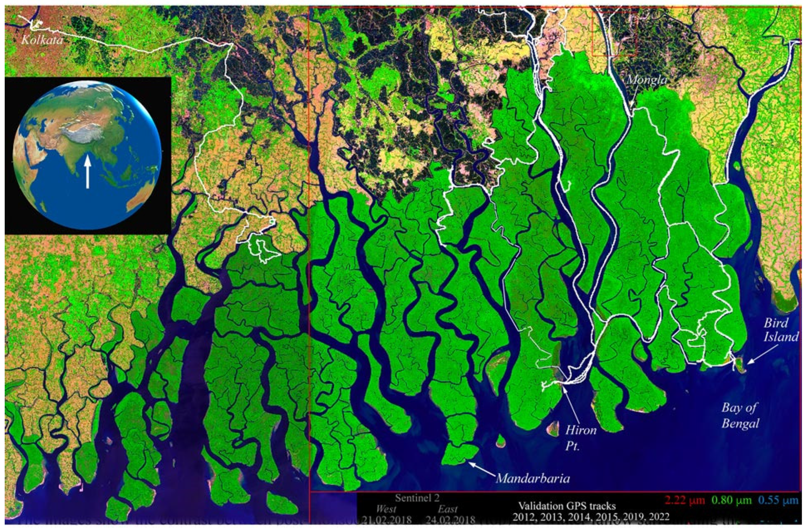
Figure 1.
Index map of the Sundarban mangrove forest at the mouths of the Ganges–Brahmaputra delta. The Sentinel 2 false color composite from 2018 shows river channel network and forest canopy cover variations. Note the contrast of the mangrove canopy with the dry season agriculture (bright green), fallow fields (tan), and aquaculture ponds (black) on embanked islands surrounding the forest. The contrast in mangrove reflectance between the eastern and western tiles is a BRDF effect due to the contrasting view geometries at the opposite edges of adjacent Sentinel 2 swaths. GPS tracks (white) show the extents of boat-based field surveys. The east–west scale is 185 km.
The objectives of this study are threefold: (1) spectroscopic characterization of mangrove reflectance across geography and season to quantify the diversity of spectral features that may be indicative of the physical properties of the canopy, (2) spatiotemporal characterization of mangrove phenology and decadal change over the entire Sundarban spanning India and Bangladesh, and (3) comparison of the spatial and temporal intersections of spectroscopic properties and the spatiotemporal phenology with geographic variations in physical properties expected to influence the variety of mangrove communities occurring across the entire Sundarban. These characterizations are intended to provide a context for understanding mangrove ecosystem form and function more generally. Both characterizations use two complementary forms of dimensionality reduction, applied in parallel with the EMIT reflectance and MODIS Enhanced Vegetation Index (EVI) time series.
2. Materials and Methods
2.1. Data
2.1.1. EMIT Reflectance
The Earth Mineral Dust Source Investigation (EMIT) is a NASA mission with the primary purpose of studying the mineralogy of dust and dust source regions using spaceborne imaging spectroscopy [12]. The EMIT imaging spectrometer has a Dyson architecture with an 11° cross-track field of view and a wide-swath (1240 samples) F/1.8 optical system. The EMIT instrument samples across a 380–2500 nm spectral range at roughly 7.4 nm and a high signal-to-noise (SNR) ratio [13]. EMIT was launched on 14 July 2022 using a SpaceX Dragon vehicle and autonomously docked to the forward-facing port of the International Space Station (ISS) [14]. EMIT data and algorithms are freely available for public use.
EMIT imaged parts of the Sundarban mangrove forest twice in December 2023 and once in April 2024 (Figure 2). The December acquisitions of the western and central Sundarban occurred 4 days apart under similar view and illumination geometries but differing atmospheric conditions. In contrast, the April acquisition of the central and eastern Sundarban occurred under significantly higher solar elevation than the December acquisitions. The substantial overlap between the 12/27 and 4/24 acquisitions allows for a comparison of the same subset of forest at near-opposite stages of the phenological cycle, which is modulated by post-monsoon greening and dry season senescence.
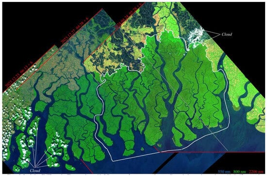
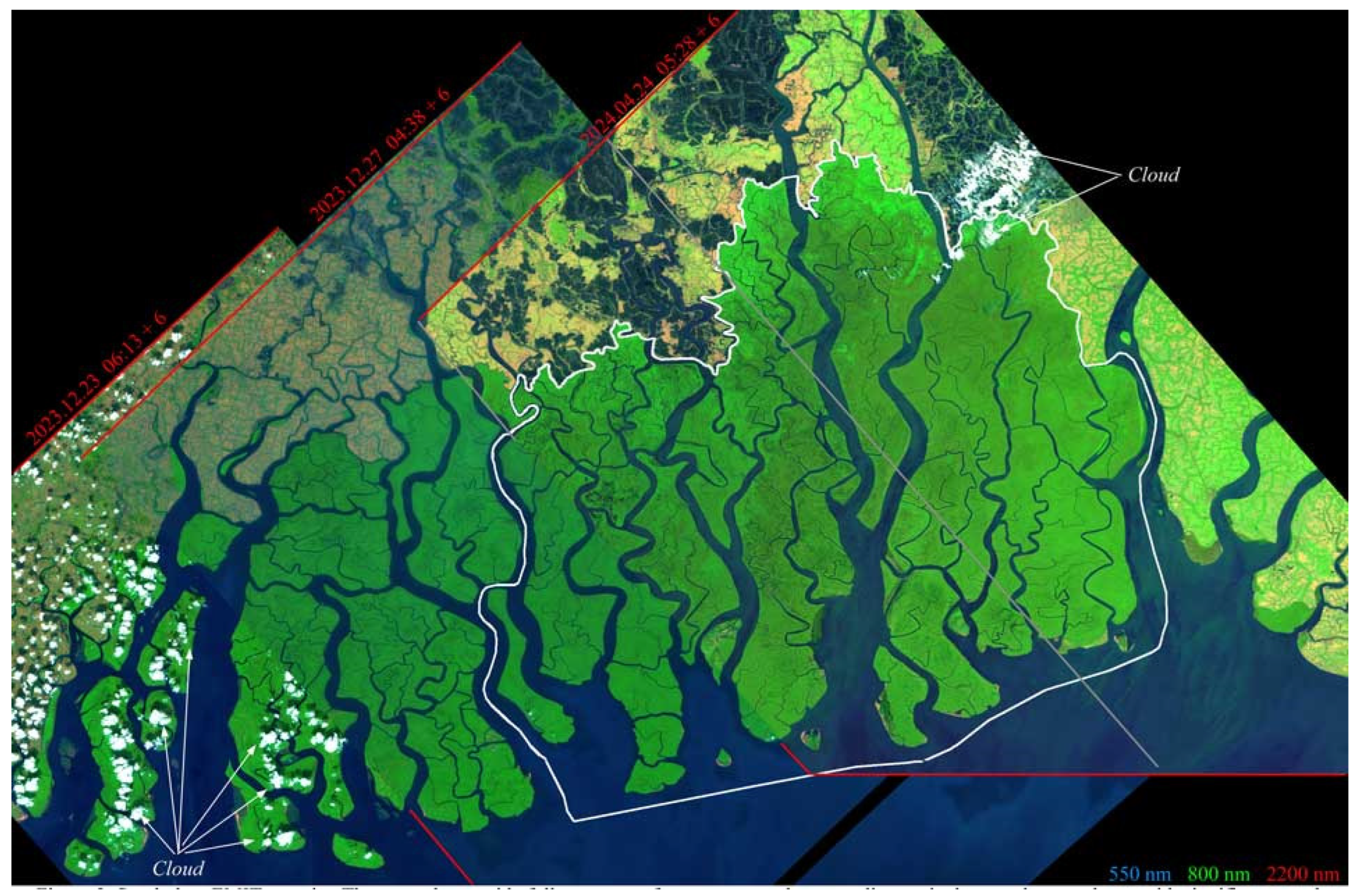
Figure 2.
Sundarban EMIT mosaic. Three swaths provide a full coverage of mangroves and surrounding agriculture and aquaculture, with significant swath overlap. Acquisition dates span nearly the full annual phenological cycle from post-monsoon in December to pre-monsoon in April. Solar zenith angles at times of acquisition range from 11.5° (04.24) to 50.5° (12.27). The white vector boundary shows the extent of the Bangladesh Sundarban, for which tree species maps are available. Acquisition times are UTC + 6 h offset.
EMIT data were downloaded free of charge from http://search.earthdata.nasa.gov/, accessed on 22 July 2024. Images were downloaded in netCDF format as Level 2A ISOFIT-corrected reflectance [15]. The ISOFIT atmospheric correction uses Bayesian Optimal Estimation [16] to produce surface reflectance spectra and Aerosol Optical Depth and column water vapor estimates at the pixel scale. Level 2 reflectance and mask files were acquired, as well as Level 1B at-sensor radiance for visual inspection.
2.1.2. MODIS EVI
MODIS data were downloaded free of charge from the International Research Institute for Climate and Society Data Library (IRIDL) at http://iridl.ldeo.columbia.edu/SOURCES/.USGS/.LandDAAC/.MODIS/.version_006/, accessed on 23 July 2024. The Enhanced Vegetation Index (EVI) layer of Version 6 of the MOD13Q1 product (MODIS/Terra Vegetation Indices 16-Day L3 Global 250 m, Sinusoidal Grid) was used. The MOD13Q1 algorithm, described in [17], builds composite images from the maximum value of the relevant spectral index for each pixel from all quality-filtered observations within a rolling 16-day window. EVI is a normalized measure of red edge amplitude that is sensitive to variations in both canopy structure and volume scattering [18]. Unlike NDVI, EVI is more robust against atmospheric effects and scales linearly with areal vegetation abundance estimates derived from spectral mixture models [19,20,21].
2.2. Methods
We use both linear and nonlinear dimensionality reduction to characterize the spectral feature space of the EMIT reflectance product and the temporal feature space of the MODIS EVI time series. The principal components of the EMIT reflectance mosaic maximize the variance partition of orthogonal dimensions of the feature space, so they are most sensitive to “global” variations in the amplitude and shape of the spectral continuum and less sensitive to more subtle variations in narrow band absorptions and continuum curvature. In contrast, the nonlinear Uniform Manifold Approximation and Projection (UMAP) algorithm preserves “local” manifold structure by maintaining the proximity of the embedding within neighborhoods of varying scales determined by the setting of an n_neighbor (nn) hyperparameter [22]. For quantitative comparisons of individual reflectance spectra, we use the Enhanced Vegetation Index (EVI) for vegetation abundance and the Normalized Difference Water Index (NDWI) for leaf water content [23].
In order to suppress the confounding effects of highly variable water reflectance in the tidal channels within the mangrove and substrate reflectance in the agricultural areas surrounding the mangrove, we mask all EMIT pixels having vegetation fractions of less than 0.18—based on the multimodal vegetation and substrate fraction distributions of the entire mosaic. Vegetation and substrate fractions are generated using linear spectral mixture analysis [24,25,26] with a single set of generalized spectral endmembers as described in [27].
Because the MODIS compositing process and pervasive cloud cover during the summer monsoon both introduce considerable noise to the EVI time series, we use a Robust Principal Component transformation [28] to separate the low-rank and sparse components of the EVI image time series. The sparse component segregates spatiotemporal transients related to nonstationary processes like monsoon cloud cover, while the low-rank component retains the spatiotemporal structure related to the annual phenological cycles of the mangrove communities [29]. The spatiotemporal feature space is characterized using the standard L2 principal components of the low-rank component image time series following the procedure described in [30] and as a 3D UMAP embedding as described above. The structure of the PC and UMAP feature spaces reveals the most distinct phenologies present in the EVI time series as temporal endmembers bounding the feature space, as well as the presence of continua between and among the bounding endmembers [31]. Both the linear (PC) and nonlinear (UMAP) embeddings provide an empirical basis for identifying the most distinct phenologies present in the data and the relationships among them.
3. Results
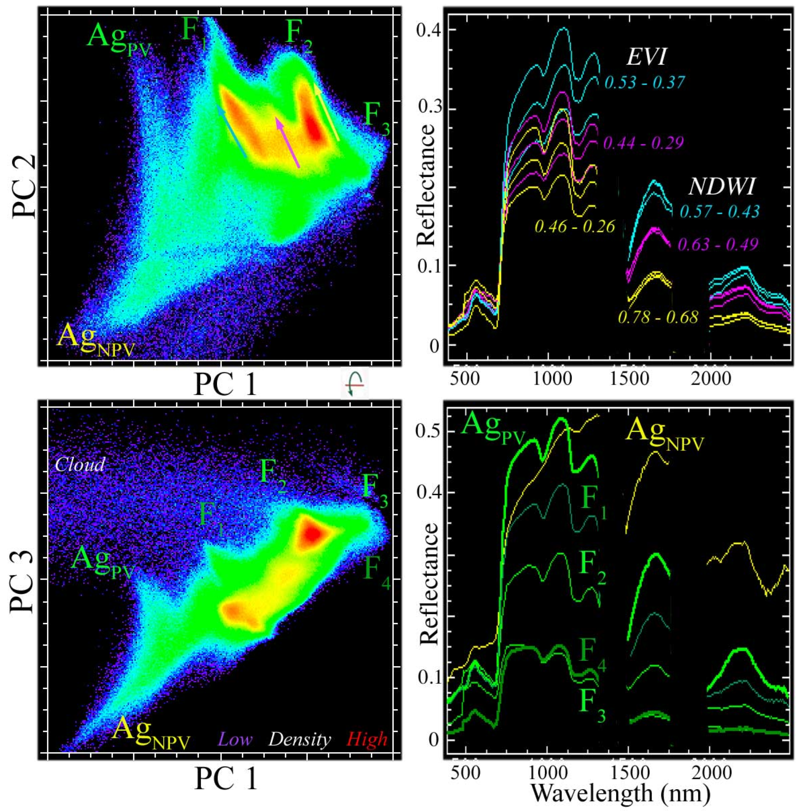
As characterized by global variance, the spectral feature space of the vegetation-masked EMIT reflectance is effectively three dimensional, with three low-order PC dimensions accounting for 95% of the total variance with all higher-order dimensions accounting for <2% each. The feature space contains distinct continua for the mangrove forest (F1–4) and for the agricultural areas (AgPV and AgNPV) on the surrounding polders (Figure 3). The forest continuum contains four distinct spectral endmembers bounding three elongate clusters representing distinct amplitude continua within the eastern, central, and western regions of the Sundarban. Each of these amplitude continua ranges from low-amplitude reflectance in the interior of the mangrove to higher-amplitude reflectance at the peripheries. Despite the fact that the western Sundarban was imaged shortly after the monsoon while the eastern Sundarban was imaged near the end of the dry season, all three distinct amplitude continua show the same progression of increasing reflectance from the interior to the peripheries of the forest.
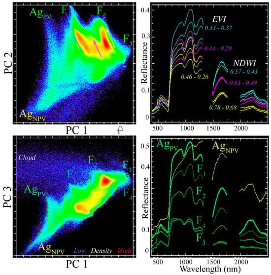
Figure 3.
Spectral feature space of the vegetation-masked Sundarban EMIT mosaic. Orthogonal projections of three low-order principal components (PCs) reveal spectral endmembers (labeled) and distinct amplitude gradients (vectors) within three clusters. Varying amplitude reflectance spectra (right) correspond to vector continua of the same color (left). While the reflectance spectra of the clusters overlap at VNIR wavelengths, each is distinct in the SWIR. The feature space spans amplitude continua with both agricultural (Ag) and forest (F) components. The agricultural continuum arises from the varying abundance of photosynthetic (PV) and non-photosynthetic (NPV) vegetation, but the amplitude of mangrove reflectance is modulated primarily by the canopy structure and varying amounts of crown shadow. There is a considerable overlap in EVI range between adjacent gradients, but a negligible overlap in NDWI range.
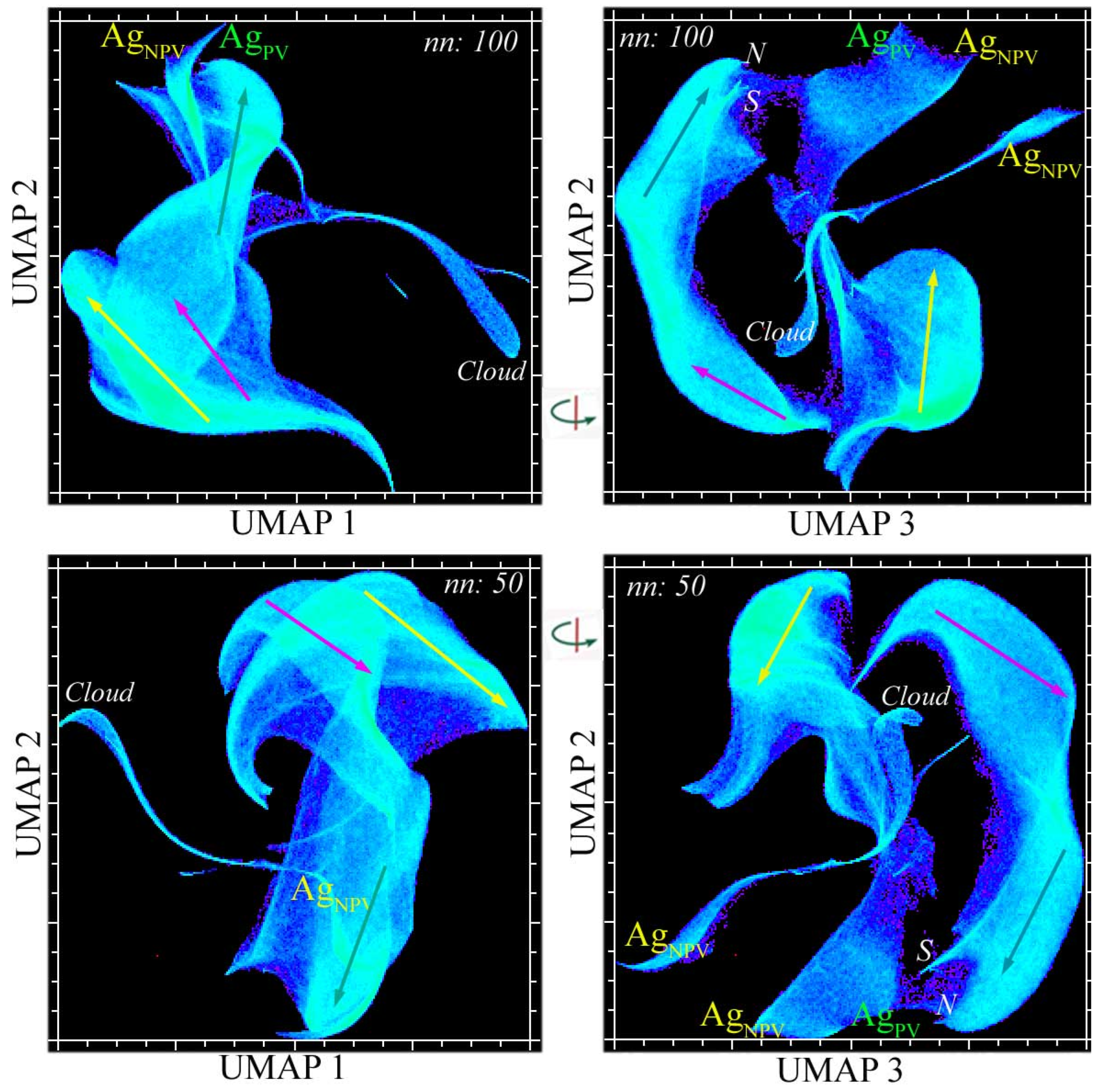
The UMAP-derived spectral feature space preserves the global structure of the PC space, despite having a more complex topology (Figure 4). Three-dimensional UMAP embeddings using different n_neighbor hyperparameter scalings (50 and 100) produce a very similar topology, with four distinct continua corresponding to those found in the PC space. However, both UMAP feature spaces reveal that the central and eastern continua in the April acquisition are isolated from the western continuum from the December acquisitions—in contrast with the PC space, which shows all four together within a single complex.
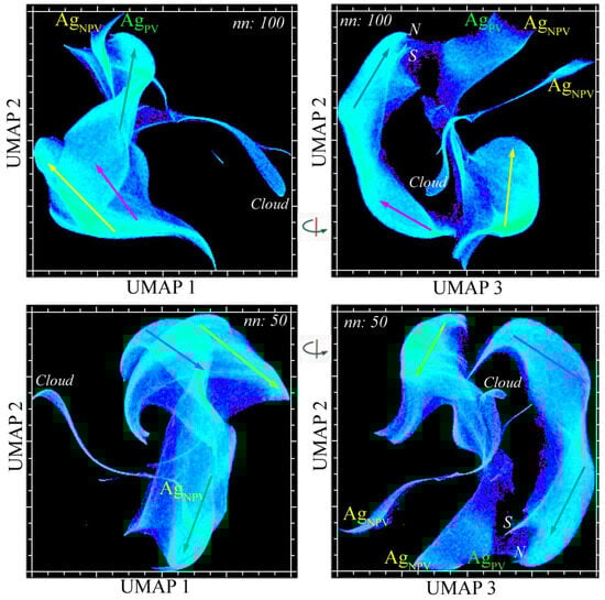
Figure 4.
Complementary spectral feature spaces of the vegetation-masked Sundarban EMIT mosaic. Orthogonal projections of two 3D UMAP embeddings (nn: 50 and 100) reveal consistent spectral endmembers (labeled) and distinct reflectance amplitude gradients (vectors) within three clusters corresponding to those in Figure 3. In both UMAP 3/2 projections (right), the western continuum (yellow) is distinct from the connected eastern and central continua (cyan and magenta). Note the bifurcation of the high-amplitude end of the eastern continuum into the northern (N) and southern (S) peripheries of the mangroves. As in the PC feature space, the surrounding agriculture forms a separate 2D continuum spanning photosynthetic and non-photosynthetic vegetation.
The reflectance spectra of the three forest continua overlap in VNIR amplitude, but are distinct in SWIR amplitude (Figure 3). The variation in VNIR amplitude is a result of differing NIR mesophyll reflectance, with little difference at visible wavelengths, which are controlled by chlorophyll absorptions. These distinctions are quantified using the Enhanced Vegetation Index (EVI) and Normalized Difference Water Index (NDWI) in Figure 3.
Spectral feature space RGB composites of the 3D PC and UMAP embeddings show a nearly identical geographic structure, despite the arbitrary orientations of their projection axes relative to the RGB coordinates. In both composites, the three reflectance amplitude continua are easily distinguished on the basis of their color gradients (Figure 5). The geographic contiguity of each of the continua in both PC and UMAP feature space composites suggests that these large-scale gradients may be a result of longitudinal variations in environmental conditions within the Sundarban. In contrast with the forest continua, the agricultural continuum spans mixtures of photosynthetic and non-photosynthetic vegetation between the post-monsoon fallow in December and the dry season crops in April.
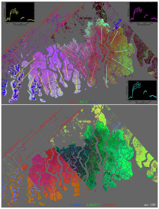
Figure 5.
PC and UMAP feature space composites. Reflectance amplitude gradients and inset spectra correspond to those in Figure 3 and Figure 4. Gradient vectors indicate a direction of increasing NIR reflectance. Composite colors are determined by 3D feature space topology in PC and UMAP spaces. The swath edge discontinuity in the center contrasts post-monsoon (west) from dry season (east) reflectance and longitudinal gradients in species composition and environmental conditions.
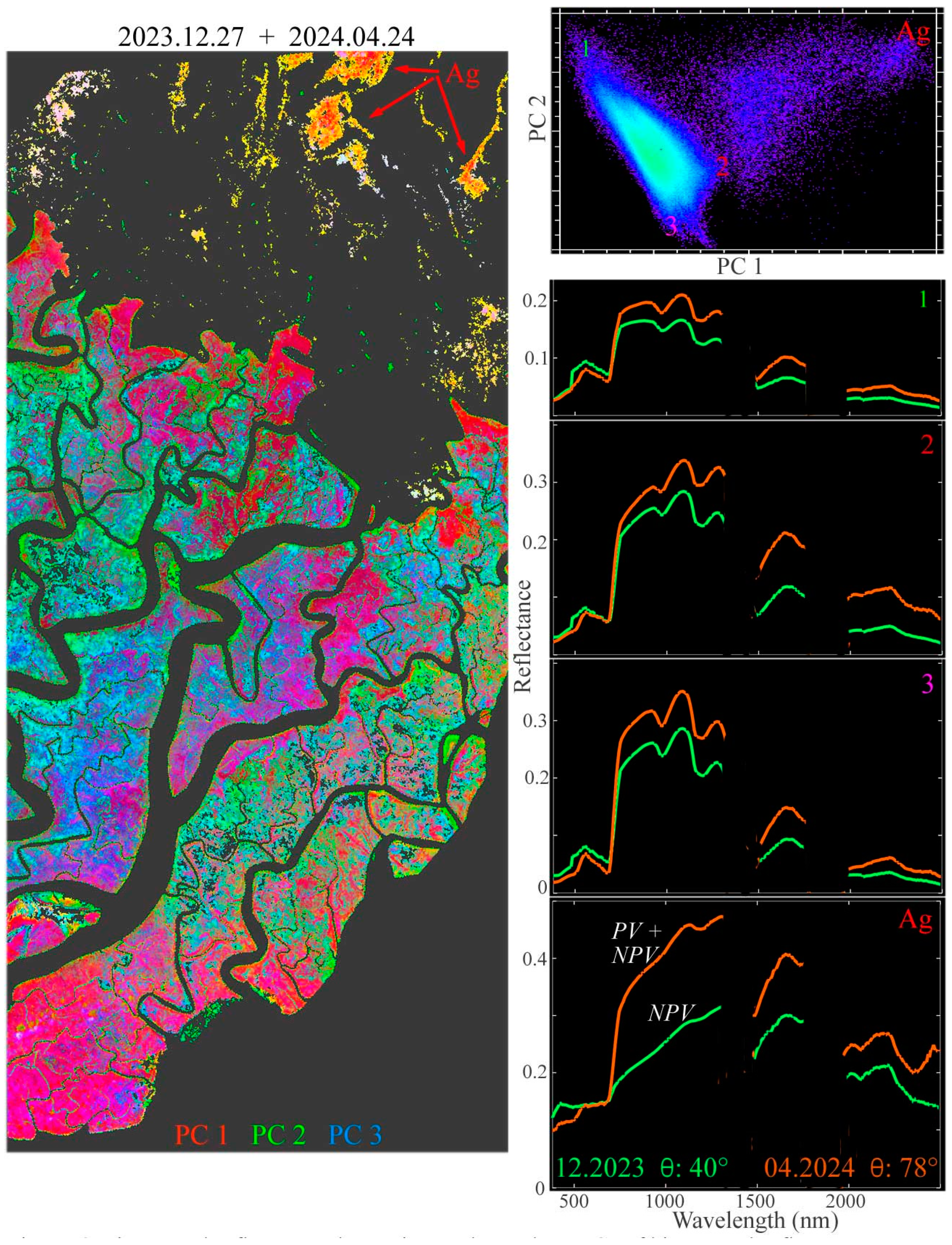
The overlap of the December 2023 swath to the west and the April 2024 swath to the east allows us for characterizing wet and dry season changes in the central Sundarban. The PC-based spectral feature space of the bitemporal stack of overlapping pixel reflectance spectra reveals three forest and one agricultural reflectance change endmembers (Figure 6). The three forest reflectance change endmembers are distinct in terms of amplitude and continuum shape, particularly in the shape of the red edge and NIR shoulder. As expected, all three change endmembers are more absorptive in the SWIR in the post-monsoon acquisition than in the dry season acquisition, as decreasing leaf water content throughout the dry season should reduce the liquid water absorptions. However, the NIR reflectance amplitude of all three change endmembers also increases from post-monsoon to dry season—in contrast with the decreasing EVI observed by (Small and Sousa 2019) using Harmonized Landsat + Sentinel time series. A comparison of the overlap between the two December acquisitions in the west with the overlap between the December and April acquisitions reveals a significantly higher Aerosol Optical Depth (AOD) for the 27 December acquisition compared with the other two. The wavelength-dependent effect of the anomalous AOD, apparently not fully corrected by the radiative transfer model, effectively increases the visible and decreases the NIR reflectance of the 12/23 acquisition, reducing its EVI accordingly. The details of this analysis are given in Appendix C.

Figure 6.
Bitemporal reflectance change in swath overlap. PCs of the bitemporal reflectance space show a continuum bounded by three endmember reflectance changes for mangrove forest and one for dry season agriculture (Ag). For each forest change endmember, SWIR liquid water absorptions are deeper in December, following the monsoon, but significantly reduced by the April dry season. In contrast, the chlorophyll absorptions in the visible change little. Coherent spatial patterns in bitemporal PC composite suggest aggregate responses to solar illumination (θ) and SWIR water absorption.
Despite the conflated phenological and atmospheric effects in the central Sundarban overlap, the bitemporal reflectance change composite of the three low-order PCs shows spatially coherent variations among the three forest change endmembers (Figure 6). This suggests that the factors driving the expected differences in leaf water content may be controlled either by local environmental conditions (e.g., surface hydrology) or by coherent variations in tree species distributions. Such conditions might also be expected to influence canopy senescence rates between the wet and dry seasons.
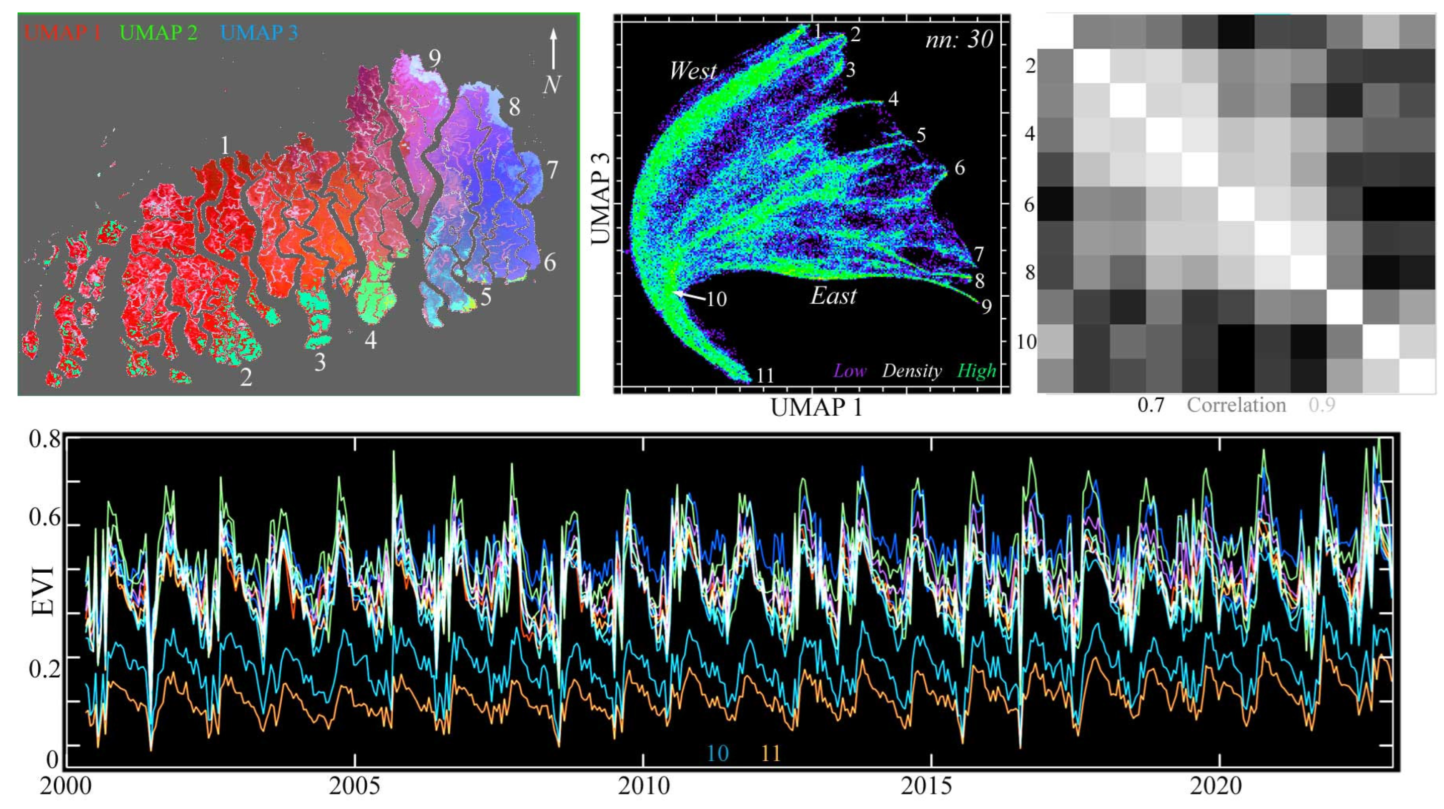
The PC-based temporal feature space of the Sundarban MODIS EVI time series is amorphous with no clear endmembers, but the UMAP-based temporal feature space shows a clear branching structure (Figure 7). The latter feature space reveals nine distinct temporal endmembers, spanning the periphery of the Sundarban longitudinally, tapering to a common branch point (10) and a single root (11). As with the single-date reflectance-based spectral feature spaces, the continua in the UMAP temporal feature space correspond to geographic continua extending from the high-amplitude EVI phenologies at the peripheries of the Sundarban to the lower-amplitude phenologies in the interior of the forest. The low-amplitude phenologies at the branch and root of the space are associated with MODIS pixels spanning shorelines and channels representing spectral mixtures of illuminated forest canopy, shadow, and water.

Figure 7.
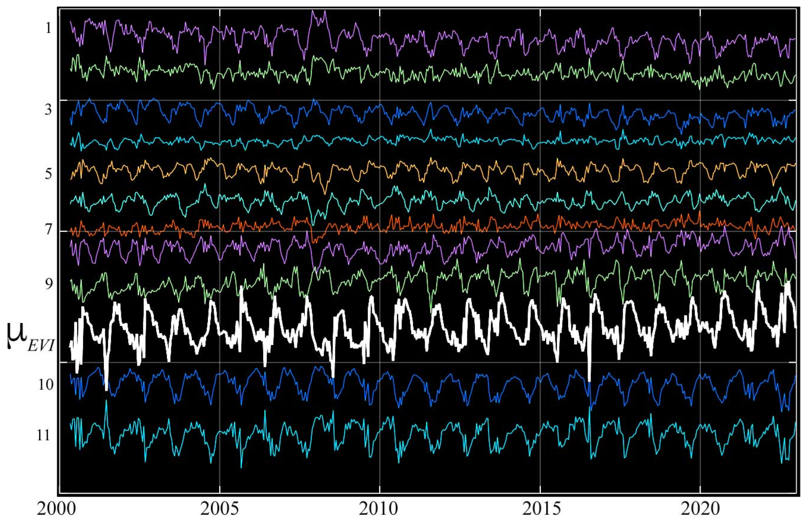
Temporal feature space of MODIS EVI time series for the entire Sundarban mangrove forest, 2000–2022. The UMAP composite (upper left) shows both N–S and E–W gradients in seasonal phenology, as well as several abrupt transitions. The 1/3 projection of the 3D UMAP feature space (upper center) has a single root (11) corresponding to lower EVI mixtures of canopy, water, and shadow at riverbanks and narrow channels within the mangrove. As EVI increases with canopy closure, the root diverges (10) into mixing trends, terminating at 9 distinct temporal endmembers. EVI time series (bottom) increase abruptly during the summer monsoon, and then decrease gradually over the rest of the year. The 9 endmembers correspond to peripheral regions of the Sundarban (upper left) with the highest post-monsoon EVI. The correlation matrix (upper right) of all 11 endmembers shows the highest correlations between geographically adjacent endmembers. The 2 lowest- (10, 11) and 2 highest (1, 9)-amplitude endmembers are less intercorrelated than those at the southern and eastern peripheries (2–8). Also apparent in the UMAP composite is the distinction between the phenological diversity of the eastern Sundarban and the more homogeneous center in the west.
As with the reflectance feature spaces, the 3D UMAP composite of the temporal feature space shows a strong contrast between the more diverse eastern and the more continuous central and western Sundarban phenology. All 11 temporal endmembers are phase-aligned with a similar asymmetric monsoon-driven phenology—yet each is distinct in the amplitude and shape of its phenological cycle (Figure 8). Among the 9 higher-amplitude temporal endmembers, 2 at the northern periphery of the Sundarban (8 and 9) are distinct from the 7 (1–7) at the southern and eastern peripheries—which have conspicuously higher correlations than the 2 at the northern periphery.
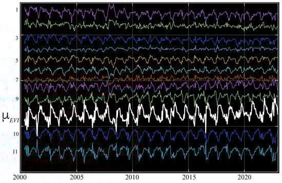
Figure 8.
Sundarban temporal endmember phenologies from the temporal feature space in Figure 7. The mean EVI (white) shows the rapid post-monsoon greening and gradual dry season senescence, while mean-removed residuals (color) of individual endmembers (offset for clarity) show a diversity of periodic excursions from the mean. As seen in Figure 7, all endmembers are phase-aligned and differ primarily in the rate and amplitude of dry season EVI decrease. Despite the considerable noise, distinct annual periodicity is apparent in all but the lowest-amplitude (e.g., 2, 4, 7) residuals—which are most similar to the mean. The largest-amplitude residuals are those from the root and branch (10, 11) of the feature space, corresponding to lower EVI associated with partial canopy cover on shorelines and small channels. Note the slight decadal increase in minimum EVI of the mean.
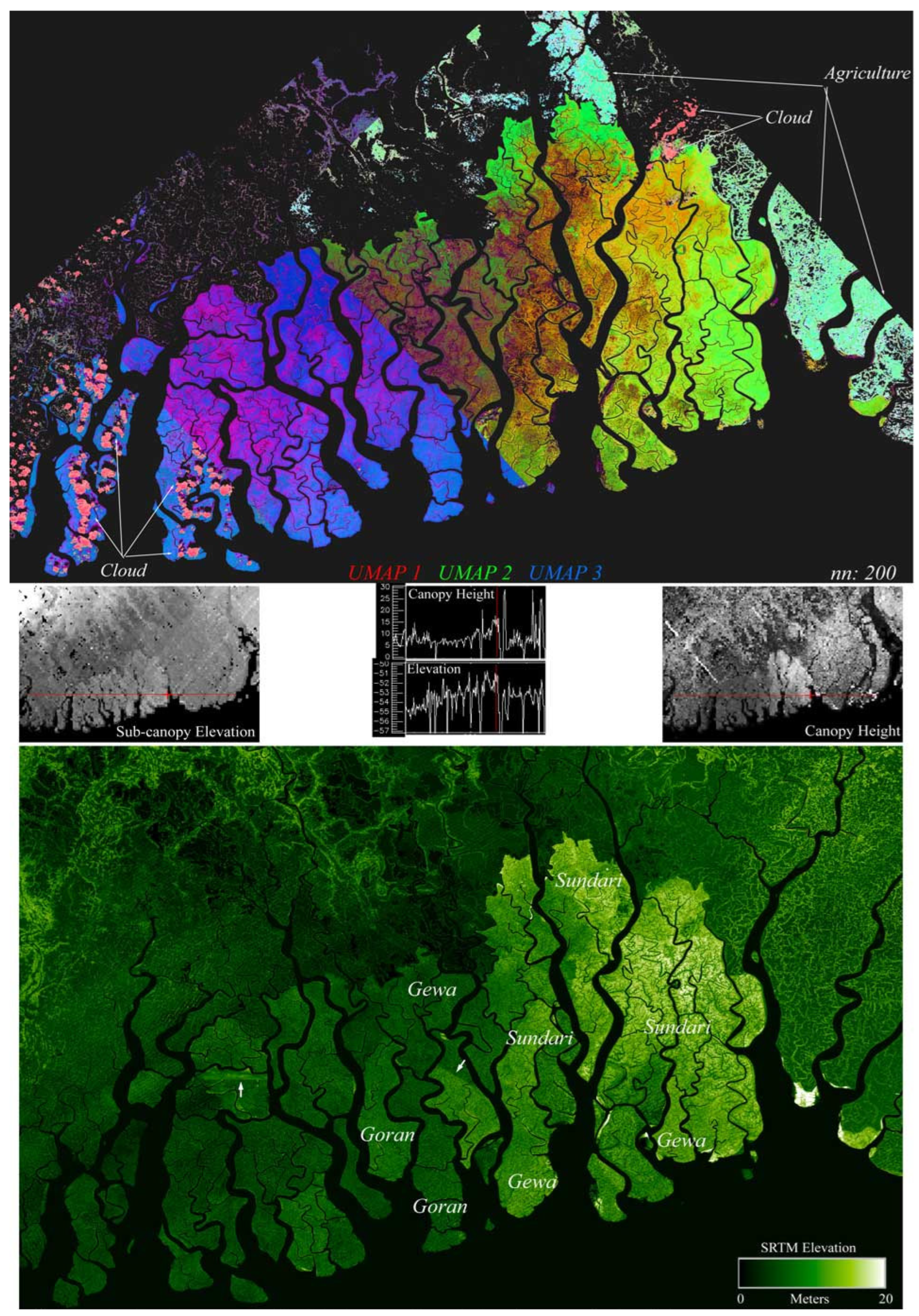
The eastern versus center + western difference in both reflectance and phenology corresponds to longitudinal gradients in both canopy height and ground elevation within the Sundarban. Kilometer resolution aggregations of GEDI LiDAR observations (https://doi.org/10.3334/ORNLDAAC/1952, accessed on 23 July 2024) reveal that the eastern Sundarban has 1–2 m higher ground elevation compared with the surrounding embanked islands (Figure 9). Canopy height estimates derived from the same GEDI LiDAR product also show a longitudinal gradient in maximum canopy height from almost 20 m in the east to less than 10 m in the west. Hence, the observed longitudinal height gradient observed in 30 m SRTM DEM elevations is a result of gradients in both sub-canopy ground elevation and canopy height.

Figure 9.
EMIT reflectance mosaic UMAP composite and elevation maps for the Sundarban and surrounding delta. GEDI LiDAR maps (center) reveal that an ongoing sediment deposition in the mangrove forest results in 1–2 m higher ground elevation in the eastern Sundarban relative to the surrounding embanked islands, which have been sediment-starved for decades. The higher SRTM elevation of the eastern Sundarban is a result of both the higher ground elevation and the greater canopy height of the tree species. Mono-species epicenters, from a Bangladesh Forest Department species map (2002), are labeled by common (local) names of tree species. Bi-species gradients compose most of the eastern Sundarban. Arrows show two SRTM swath discontinuity artifacts, which are distinct from the numerous height discontinuities occurring across channels.
4. Discussion
4.1. Spectroscopic Phenology
The primary result of this analysis is the strong geographic correspondence between the spectral and phenological endmembers and gradients within the Sundarban mangrove forest. Both EMIT reflectance and MODIS EVI have multiple distinct high amplitude endmembers occupying the peripheries of the Sundarban with amplitude gradients extending to the interior. The EMIT spectral feature spaces reveal three distinct amplitude gradients corresponding to the eastern, central, and western Sundarban. While the western Sundarban was imaged much later in the phenological cycle, it shows the same outward progression of reflectance amplitude seen in the eastern and central Sundarban. The UMAP temporal feature space reveals a similar longitudinal structure with a continuum spanning distinct eastern and western limbs, all converging to a common branch point and lower amplitude root. A multiscale UMAP analysis using multiple n_neighbor hyperparameter settings reveals an even more strongly ternary structure (see Appendix A for details).
While the temporal feature space does not distinguish the central Sundarban as clearly as the spectral feature spaces do, the longitudinal and lesser latitudinal gradients are conspicuous in their similarity. This suggests that the physical factors controlling reflectance amplitude at either phase of the phenological cycle may also control geographic variations of the amplitude of the cycle itself. However, the primary limitation of this study is the contrasting timing of the eastern and western EMIT acquisitions. Verifying these inferences will require simultaneous spectroscopic imaging of the entire Sundarban at multiple points in its phenological cycle. In comparison to traditional phenology analysis using individual vegetation indices derived from broadband multispectral sensors, repeat spectroscopic imaging of ecosystems like mangroves offers the opportunity to resolve multiple absorption-specific effects on canopy reflectance (e.g., chlorophyll and water) that may respond to different environmental factors simultaneously.
4.2. Mangrove Community Composition
Tree species composition, canopy height, and subcanopy ground elevation show similar geographic gradients to those observed in the reflectance amplitude and phenology. This suggests that geographic variations in surface hydrology, sediment supply, tidal flushing, and nutrient input may all impact both the reflectance amplitude and phenological gradients observed within the Sundarban. In terms of physical properties, we expect the distinct gradients in NIR reflectance amplitude to be controlled primarily by canopy closure, crown density, and foliar volume scattering, while the corresponding differences in SWIR reflectance amplitude driving the distinction between the eastern, central, and western gradients should be more sensitive to the aggregate leaf water content of the canopy. Both of these physical properties could be strongly influenced by both tree species composition and the environmental factors mentioned above.
The most conspicuous and unexpected revelation of this combined analysis is the distinct radial amplitude gradients of both spectroscopic surface reflectance and EVI phenology in the eastern, central, and western Sundarban. Based on our experience of over a decade of in situ field observations within the Bangladesh Sundarban, we conjecture that the greater reflectance and phenological amplitude of the peripheral regions of the eastern Sundarban may be, in part, a fertilization effect from the agricultural and aquacultural effluent of the surrounding polders. Both the agriculture and aquaculture cycles, occurring for far longer than the duration of either the MODIS or EMIT satellite observation record [32], yield nutrients that may be present in significantly higher concentrations in the river water flowing into the Sundarban at its northern and eastern peripheries than in the tidally driven inflow from the Bay of Bengal to the south. However, this conjecture begs the question of why the phenological feature space also reveals the southernmost islands on the Bay of Bengal as having distinct phenologies from the northern and eastern peripheries. We further conjecture that the substrate composition of the southernmost islands may influence both the tree species composition and the surface hydrology in ways that may be manifest in the aggregate phenology. Specifically, the much greater abundance of sand and coarse silt delivered by the high energy sedimentary environments (e.g., beaches) on the Bay of Bengal may impact the rooting structure and nutrient availability in those environments. The effects of high energy wave action on sediment deposition and reorganization are further exacerbated by the impact of cyclones, which are a regular occurrence on the Bay of Bengal. These southernmost islands are distinct from the interior platforms farther north in both elevation and tree species composition. The latter is confirmed by the species map and our own field observations. The tidal currents that extend throughout the interior Sundarban generally lack the energy to deposit significant amounts of sand and coarse silt on the platform interiors, thereby giving rise to the deep mud substrates that characterize most of the subaerial Sundarban. These conjectures are consistent with our own field observations (Figure 10), and those of our colleagues, but could easily be tested by sediment coring and aqueous geochemical sampling within the channels and platforms of the Sundarban.
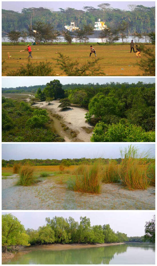
Figure 10.
Field photos illustrate the forest diversity of the Bangladesh Sundarban. The northeast Sundarban (top) reaches canopy heights of 25 m, in contrast with the surrounding embanked islands, which are often below sea level. The sand-dominant islands of the southeast (upper center) are intertidal only around their peripheries and contain different tree species from the rest of the Sundarban. The vegetation gradient of Bird Island on the Bay of Bengal (lower center) illustrates the succession of grasses, shrubs, and trees that colonize sand-dominant islands. River channel networks (bottom) continually deliver silt and mud to intertidal islands throughout the Sundarban. Photos © C. Small 2012–2022.
While the accuracy of the tree species map of the interior Bangladesh Sundarban is unknown (to us), species identifications made from the extensive channel network (e.g., Figure 10) do lend credence to the visual interpretation of the aerial imagery on which the map is based. We are aware of no comparable tree species mapping available for the western Sundarban in India, so we have no basis for speculation on its diversity or effect on reflectance amplitude or phenology. The diversity of reflectance and phenology patterns revealed by the maps in Figure 5, Figure 6, Figure 7 and Figure 9 could be used to guide a focused sampling of mangrove community composition within platform interiors, particularly in areas where steep gradients or even discrete transitions are revealed.
4.3. Limitations
The bitemporal overlap in the central Sundarban conflates temporal variations in phenological phase, illumination geometry, and atmospheric effects. This sharply limits the inference we can draw from this comparison. However, the spatial contiguity of the bitemporal changes in reflectance within the overlap suggests potential sub-kilometer scale variations in phenology consistent with those observed in the central Sundarban (Small and Sousa 2019).
4.4. Future Considerations
As mentioned above, the PC and UMAP feature space composites of this study could be used to guide field observations of both tree species and substrate properties. We are currently analyzing river discharge time series for the rivers feeding the northern and eastern Sundarban to determine if there is any consistency in interannual variations in discharge and phenology. Of at least equal importance will be a comparative analyses of a full Sundarban coverage of spectroscopic imagery at different phases of the phenological cycle. Despite the EMIT mission’s focus on arid environments and dust-related processes, we are hopeful that additional acquisitions of the Sundarban, and other mangroves, may facilitate an extension of the combined spectral + phenological characterization presented here. To our knowledge, this analysis approach has not yet been performed in any other mangrove systems, largely due to the novelty of EMIT data and the spatial extent of the EMIT coverage mask. Further EMIT acquisitions could serve to replicate this analysis approach in other mangroves worldwide, eventually serving as a basis for a global comparative analysis of joint spectroscopic and phenological diversity.
5. Conclusions
Spatial gradients in EMIT reflectance amplitude coincide closely with spatial gradients in MODIS EVI phenology throughout the Sundarban mangrove forest. The reflectance amplitude gradients arise from a combination of canopy structure (NIR) and leaf water content (SWIR). Phenological amplitude gradients reflect geographic variations in the rate of post-monsoon greening and dry season senescence. Both reflectance and phenology gradients extend radially outward from the interior of the mangrove forest to its peripheries and vary longitudinally from east to west with a difference in sub-canopy ground elevation and canopy height. While three distinct reflectance gradients are observed for the eastern, central, and western Sundarban, the bitemporal coverage of the EMIT acquisitions introduces a temporal discontinuity between the post-monsoon coverage in the west and the dry season coverage in the east. Hence, the western gradient may be partially a result of the difference in phenological phase, while the eastern and central gradients are distinct within a single acquisition. A simultaneous imaging of the entire Sundarban may reveal that the central gradient could extend farther west, as is observed in the phenological gradients that bifurcate into a continuum of longitudinal gradients from interior to periphery. Four distinct spectral endmembers are observed in the EMIT spectral feature space, whereas 10 distinct temporal endmembers are observed in the MODIS EVI temporal feature space. All of the temporal endmembers are phase-aligned but differ in the rate and extent of senescence during the dry season. We conjecture that these distinct phenologies may result from the geographic variations in platform height, surface hydrology, salinity, and species composition of the diversity of mangrove communities present in the Sundarban. Simultaneous spectroscopic imaging of the entire Sundarban over the course of the phenological cycle may allow for competing effects of canopy closure and leaf water content to be distinguished independently.
Author Contributions
Conceptualization, C.S.; methodology, C.S. and D.S.; validation, C.S. and D.S.; formal analysis, C.S. and D.S.; investigation, C.S. and D.S.; resources, C.S. and D.S.; data curation, C.S. and D.S.; writing—original draft preparation, C.S.; writing—review and editing, C.S. and D.S.; visualization, C.S. and D.S.; funding acquisition, D.S. and C.S. All authors have read and agreed to the published version of the manuscript.
Funding
The authors gratefully acknowledge funding from the NASA EMIT Science and Applications Team Program (Grant # 80NSSC24K0861). D.S. additionally acknowledges funding from the USDA NIFA Sustainable Agroecosystems program (Grant #2022-67019-36397), the USDA AFRI Rapid Response to Extreme Weather Events Across Food and Agricultural Systems program (Grant #2023-68016-40683), the NASA Land-Cover/Land Use Change program (Grant #NNH21ZDA001N-LCLUC), the NASA Remote Sensing of Water Quality program (Grant #80NSSC22K0907), the NASA Applications-Oriented Augmentations for Research and Analysis Program (Grant #80NSSC23K1460), the NASA Commercial Smallsat Data Analysis Program (Grant #80NSSC24K0052), the NASA FireSense airborne science program (Grant # 80NSSC24K0145), the California Climate Action Seed Award Program, and the NSF Signals in the Soil program (Award #2226649).
Data Availability Statement
All data used in the manuscript are publicly available at the links given above.
Acknowledgments
C.S. gratefully acknowledges the support of the Lamont–Doherty Earth Observatory of Columbia University. The authors thank Phil Brodrick for useful comments about the EMIT L2 retrieval.
Conflicts of Interest
The authors declare no conflicts of interest.
Appendix A. Multiscale UMAP Characterization
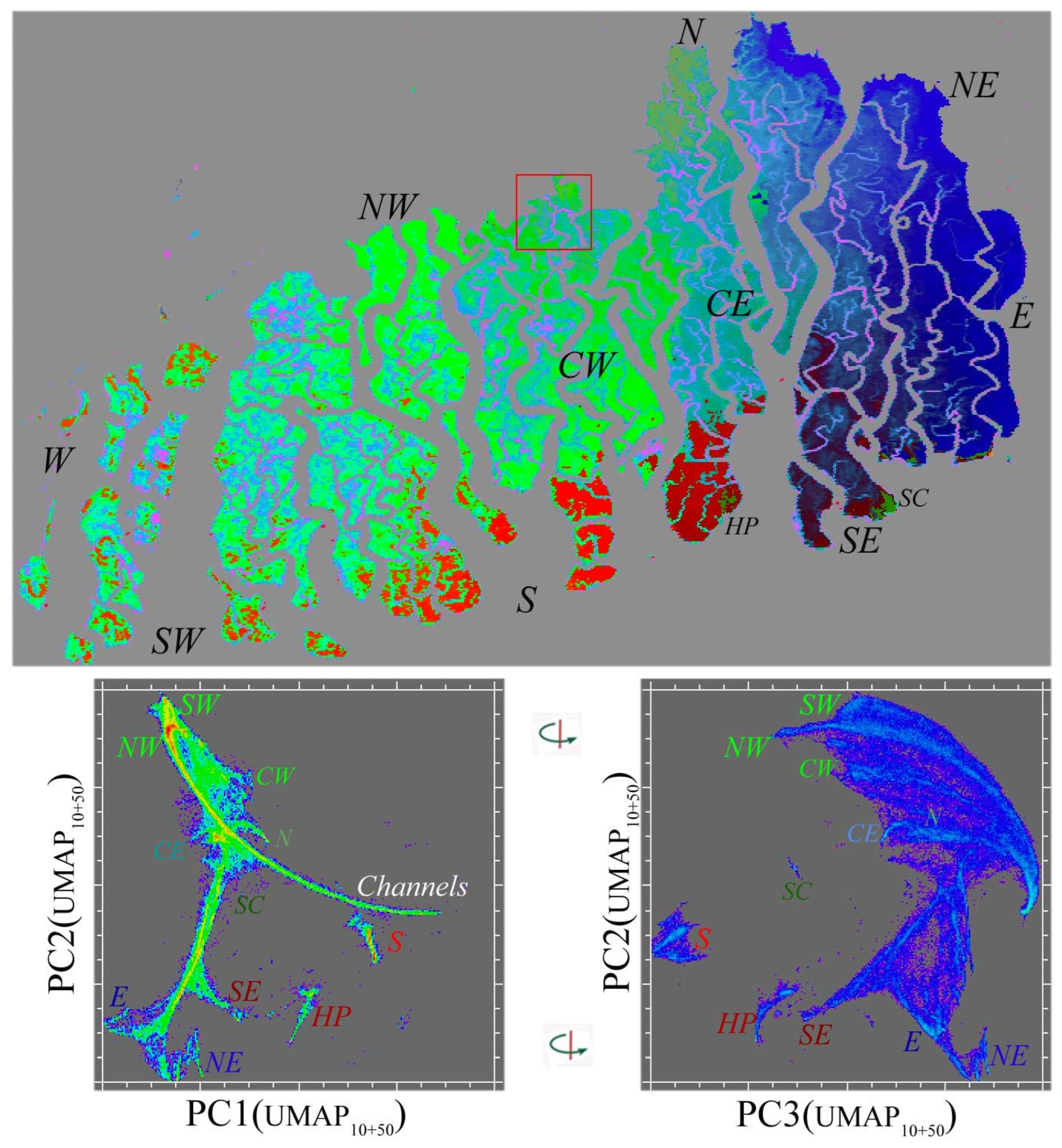
The degree to which a local and global feature space structure is preserved by the UMAP projection is most strongly influenced by the n neighbor (nn) hyperparameter. For the EMIT spectral feature space, this is illustrated in Figure 4 with clear topological similarities preserved for different nn values producing distinct embeddings. The MODIS EVI temporal feature space is more sensitive to the nn scaling. The intermediate nn value of 30 used for the feature space rendering in Figure 7 yields an easily interpreted fan structure with 10 distinct temporal endmembers clearly resolved. An alternative approach to preserving a multiscale structure is to combine 3D UMAP renderings for different nn settings in a higher dimensional sequence of UMAP embedding dimensions. Figure A1 shows orthogonal projections of the two low-order principal components of 3D projections using nn 10 and 50. The ternary structure in the 1–2 projection clearly reveals the northern and southern periphery limbs with several distinct endmembers for each, as well as the common root corresponding to lower EVI channels and shorelines within the mangrove. The southernmost islands on the Bay of Bengal (e.g., SC and HP) have phenologies completely distinct from this continuum, which is consistent with the different tree species assemblages and surface hydrology of the sand-rich substrates, in contrast with the interior of the forest, which comprises intertidal mud and silt dominant substrates.

Figure A1.
Multiscale UMAP temporal feature space with 3D PC(UMAP10+50) composite for MODIS EVI phenology. The low-order PCs of two 3D UMAP embeddings with contrasting n neighbor scales (nn: 10 and 50) preserve both the global scale limb structure and the finer scale clusters that are both phenologically and geographically distinct—including anomalous tree species assemblages at Hiron Point (HP) and Shelar Char (SC) on the Bay of Bengal shorelines. Compare the map structure with the maps in Figure 5 and Figure 7. Manifold density and UMAP color scale equivalent to those in Figure 7.
Appendix B. Robust Principal Component Analysis of MODIS EVI
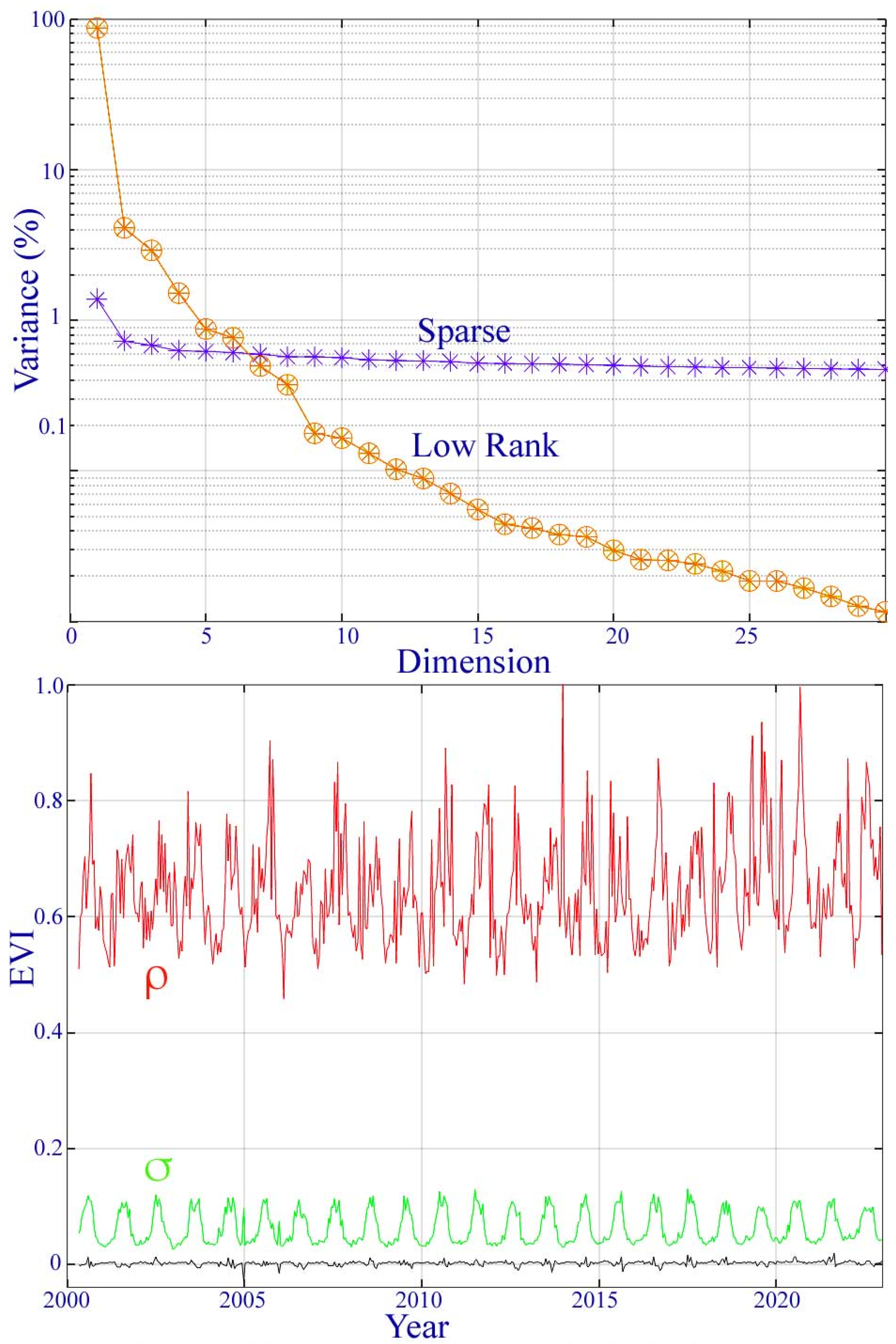
A singular value decomposition of the low-rank and sparse components of the MODIS EVI time series yields the variance partition of each from their singular values. The low-rank component can be represented with fewer than four dimensions, while the variance of the sparse component is nearly equally distributed over all dimensions—consistent with zero mean uncorrelated noise.
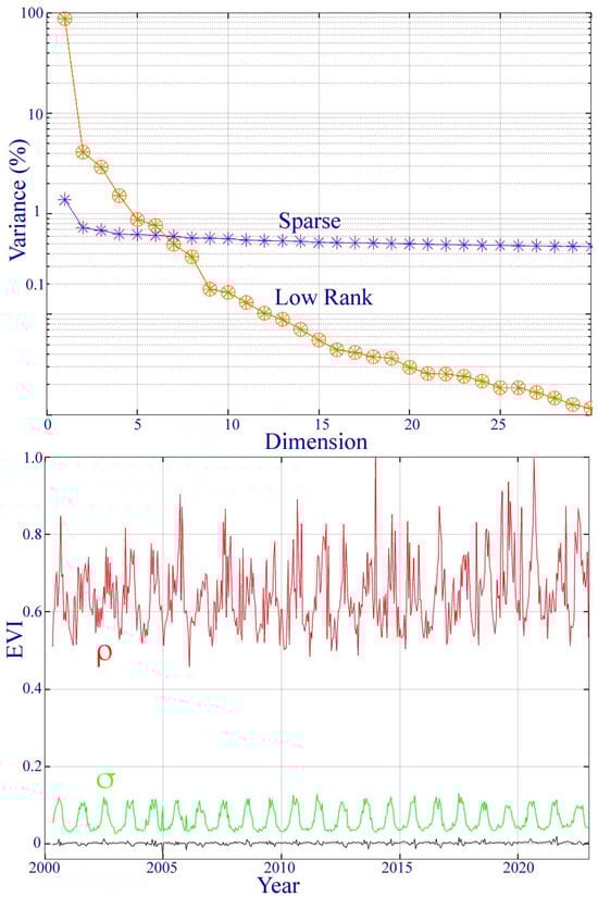
Figure A2.
Variance partition and sparse component distribution for the MODIS EVI phenology of the Ganges–Brahmaputra delta. The singular values (top) of the low-rank component suggest that the temporal feature space is effectively 4D (>1%) with 96% of the total variance, while the sparse component has a nearly uniform noise floor over all dimensions. The spatial standard deviation (σ) and range (ρ) of the sparse component peak during the monsoon as a result of a transient cloud cover.
Appendix C. Atmospheric Effects
Comparing visible composites for the overlap regions of the three EMIT acquisitions illustrates the more pervasive atmospheric scattering on the 12/27 acquisition. The mean and standard deviation of the difference spectra illustrate the wavelength dependence of this uncorrected atmospheric effect. The net result of the scattering is an increase in visible reflectance and decrease in NIR reflectance, effectively reducing the EVI for 12/27 while not affecting the SWIR absorptions.
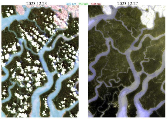
Figure A3.
Coregistered overlap between 12.23 and 12.27 EMIT acquisitions. Natural color composites illustrate the difference in aerosol optical depth with a reduced dynamic range and a greater adjacency effect on 12.27.
Figure A3.
Coregistered overlap between 12.23 and 12.27 EMIT acquisitions. Natural color composites illustrate the difference in aerosol optical depth with a reduced dynamic range and a greater adjacency effect on 12.27.
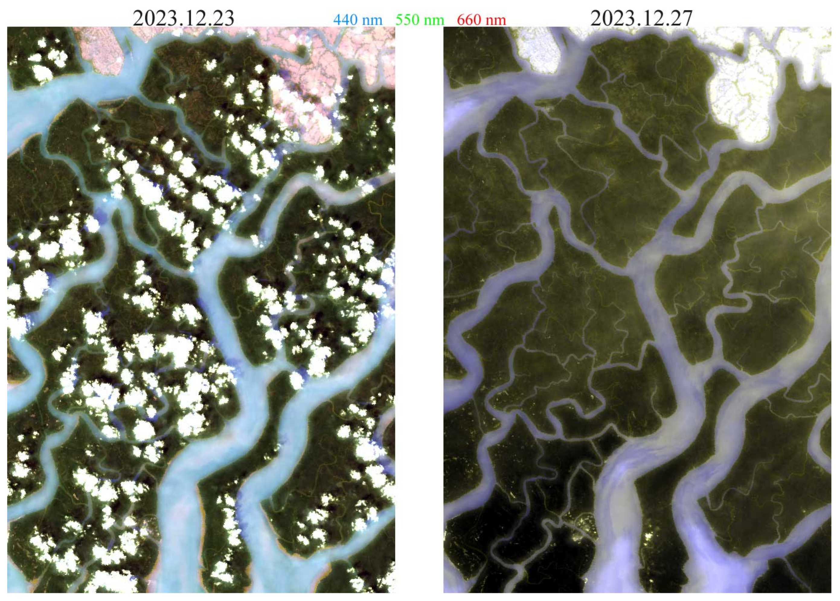
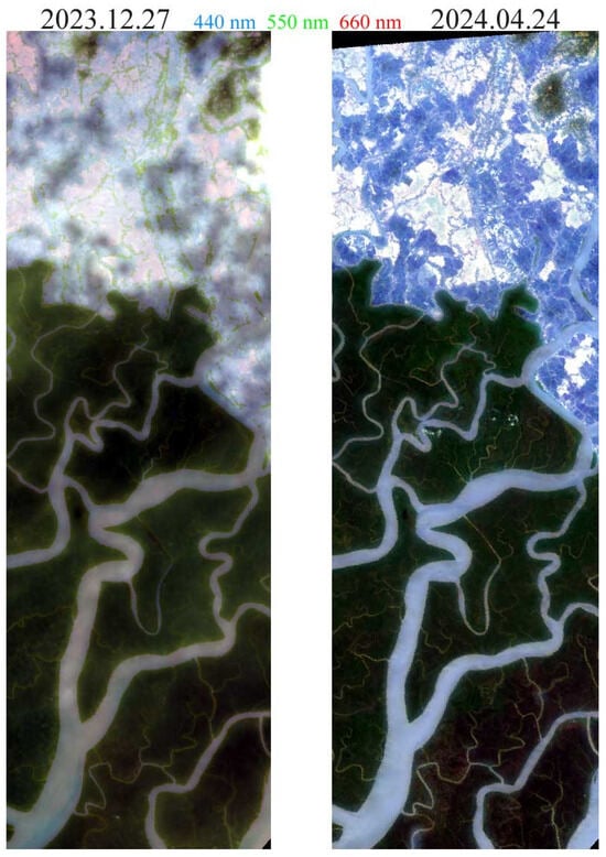
Figure A4.
Coregistered overlap between 12.27 and 04.24 acquisitions. Natural color composites show the difference in aerosol optical depth with reduced dynamic range and greater adjacency effect on 12.27.
Figure A4.
Coregistered overlap between 12.27 and 04.24 acquisitions. Natural color composites show the difference in aerosol optical depth with reduced dynamic range and greater adjacency effect on 12.27.

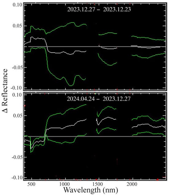
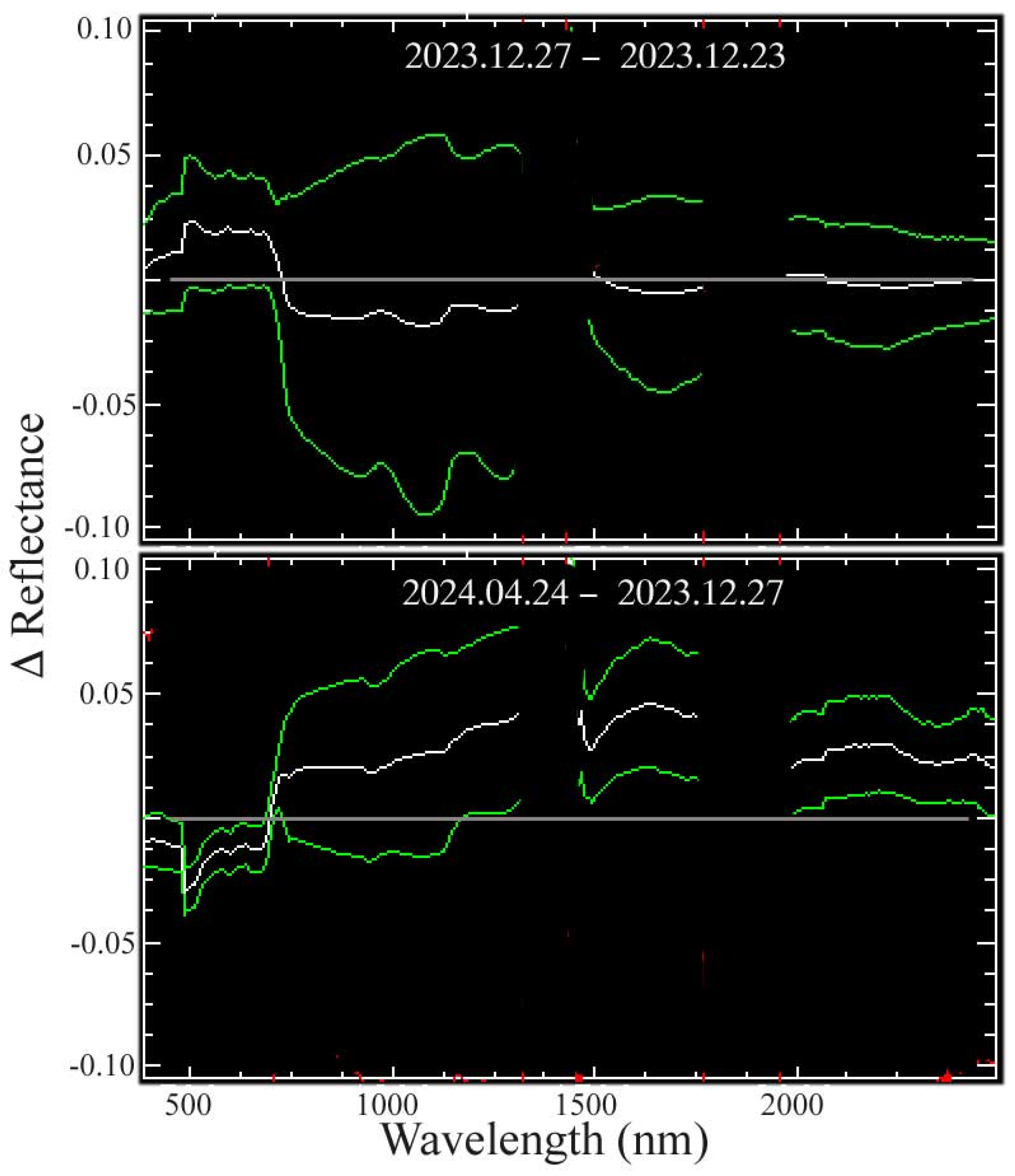
Figure A5.
Apparent change in reflectance for overlaps on 12.23, 12.27, and 04.24. The mean (white) ± 1 standard deviation (green) of all vegetation spectra in each swath overlap show the effects of residual atmospheric scattering on 12.27 and actual changes in illumination and leaf water content on 04.24. The December 23 and 27 difference suggests short wavelength-dependent scattering on 12.27 with increased visible and reduced NIR but negligible change in SWIR wavelengths. In contrast, a greater VNIR scatter on 12.27 is manifested as a reduced visible and increased NIR scatter relative to 04.24. The reduced leaf water content on 04.24 results in greater SWIR residual from reduced H2O absorption after the 4-month dry season. A higher solar elevation in April also contributes to higher NIR and SWIR reflectance.
References
- Menéndez, P.; Losada, I.J.; Torres-Ortega, S.; Narayan, S.; Beck, M.W. The Global Flood Protection Benefits of Mangroves. Sci. Rep. 2020, 10, 1–11. [Google Scholar] [CrossRef] [PubMed]
- Sandilyan, S.; Kathiresan, K. Mangrove Conservation: A Global Perspective. Biodivers. Conserv. 2012, 21, 3523–3542. [Google Scholar] [CrossRef]
- Worthington, T.A.; Zu Ermgassen, P.S.; Friess, D.A.; Krauss, K.W.; Lovelock, C.E.; Thorley, J.; Tingey, R.; Woodroffe, C.D.; Bunting, P.; Cormier, N. A Global Biophysical Typology of Mangroves and Its Relevance for Ecosystem Structure and Deforestation. Sci. Rep. 2020, 10, 14652. [Google Scholar] [CrossRef]
- Donato, D.C.; Kauffman, J.B.; Murdiyarso, D.; Kurnianto, S.; Stidham, M.; Kanninen, M. Mangroves among the Most Carbon-Rich Forests in the Tropics. Nat. Geosci. 2011, 4, 293–297. [Google Scholar] [CrossRef]
- Wang, L.; Jia, M.; Yin, D.; Tian, J. A Review of Remote Sensing for Mangrove Forests: 1956–2018. Remote Sens. Environ. 2019, 231, 111223. [Google Scholar] [CrossRef]
- Giri, C. Observation and Monitoring of Mangrove Forests Using Remote Sensing: Opportunities and Challenges. Remote Sens. 2016, 8, 783. [Google Scholar] [CrossRef]
- Giri, C.; Ochieng, E.; Tieszen, L.L.; Zhu, Z.; Singh, A.; Loveland, T.; Masek, J.; Duke, N. Status and Distribution of Mangrove Forests of the World Using Earth Observation Satellite Data. Glob. Ecol. Biogeogr. 2011, 20, 154–159. [Google Scholar] [CrossRef]
- Simard, M.; Fatoyinbo, L.E.; Pinto, N. Mangrove Canopy 3D Structure and Ecosystem Productivity Using Active Remote Sensing. Remote Sens. Coast. Environ. 2010, 61–78. [Google Scholar]
- Giri, C.; Pengra, B.; Zhu, Z.; Singh, A.; Tieszen, L.L. Monitoring Mangrove Forest Dynamics of the Sundarbans in Bangladesh and India Using Multi-Temporal Satellite Data from 1973 to 2000. Estuar. Coast. Shelf Sci. 2007, 73, 91–100. [Google Scholar] [CrossRef]
- Chowdhury, M.S.; Hafsa, B. Multi-Decadal Land Cover Change Analysis over Sundarbans Mangrove Forest of Bangladesh: A GIS and Remote Sensing Based Approach. Glob. Ecol. Conserv. 2022, 37, e02151. [Google Scholar] [CrossRef]
- Opena, F.T.; Versoza, C.G.; Mohaiman, R.; Akhter, M. Sundarban Reserved Forest; Bangladesh Forest Department: Dhaka, Bangladesh, 2002.
- Green, R.O.; Thompson, D.R.; EMIT Team. NASA’s Earth Surface Mineral Dust Source Investigation: An Earth Venture Imaging Spectrometer Science Mission. In Proceedings of the 2021 IEEE International Geoscience and Remote Sensing Symposium IGARSS, Brussels, Belgium, 11–16 July 2021; pp. 119–122. [Google Scholar]
- Bradley, C.L.; Thingvold, E.; Moore, L.B.; Haag, J.M.; Raouf, N.A.; Mouroulis, P.; Green, R.O. Optical Design of the Earth Surface Mineral Dust Source Investigation (EMIT) Imaging Spectrometer. In Proceedings of the Imaging Spectrometry XXIV: Applications, Sensors, and Processing, Online, 22 August 2020; Volume 11504, p. 1150402. [Google Scholar]
- LPDAAC EMIT Data Resources 2023. Available online: https://lpdaac.usgs.gov/resources/e-learning/emit-data-resources/ (accessed on 23 July 2024).
- Green, R. EMIT L2A Estimated Surface Reflectance and Uncertainty and Masks 60 m V001 2022. Available online: https://data.nasa.gov/dataset/EMIT-L2A-Estimated-Surface-Reflectance-and-Uncerta/hxkv-n8p3/about_data (accessed on 23 July 2024).
- Thompson, D.R.; Natraj, V.; Green, R.O.; Helmlinger, M.C.; Gao, B.-C.; Eastwood, M.L. Optimal Estimation for Imaging Spectrometer Atmospheric Correction. Remote Sens. Environ. 2018, 216, 355–373. [Google Scholar] [CrossRef]
- Huete, A.; Justice, C.; Van Leeuwen, W. MODIS Vegetation Index (MOD13). Algorithm Theor. Basis Doc. 1999, 3, 295–309. [Google Scholar]
- Huete, A.; Didan, K.; Miura, T.; Rodriguez, E.P.; Gao, X.; Ferreira, L.G. Overview of the Radiometric and Biophysical Performance of the MODIS Vegetation Indices. Remote Sens. Environ. 2002, 83, 195–213. [Google Scholar] [CrossRef]
- Small, C.; Milesi, C. Multi-Scale Standardized Spectral Mixture Models. Remote Sens. Environ. 2013, 136, 442–454. [Google Scholar] [CrossRef]
- Sousa, D.; Small, C. Global Cross-Calibration of Landsat Spectral Mixture Models. Remote Sens. Environ. 2017, 192, 139–149. [Google Scholar] [CrossRef]
- Sousa, D.; Small, C. Which Vegetation Index? Benchmarking Multispectral Metrics to Hyperspectral Mixture Models in Diverse Cropland. Remote Sens. 2023, 15, 971. [Google Scholar] [CrossRef]
- McInnes, L.; Healy, J.; Melville, J. Umap: Uniform Manifold Approximation and Projection for Dimension Reduction. arXiv 2018, arXiv:1802.03426. [Google Scholar]
- Gao, B.-C. NDWI—A Normalized Difference Water Index for Remote Sensing of Vegetation Liquid Water from Space. Remote Sens. Environ. 1996, 58, 257–266. [Google Scholar] [CrossRef]
- Adams, J.B.; Smith, M.O.; Johnson, P.E. Spectral Mixture Modeling: A New Analysis of Rock and Soil Types at the Viking Lander 1 Site. J. Geophys. Res. Solid Earth 1986, 91, 8098–8112. [Google Scholar] [CrossRef]
- Smith, M.O.; Ustin, S.L.; Adams, J.B.; Gillespie, A.R. Vegetation in Deserts: I. A Regional Measure of Abundance from Multispectral Images. Remote Sens. Environ. 1990, 31, 1–26. [Google Scholar] [CrossRef]
- Gillespie, A.; Smith, M.; Adams, J.; Willis, S.; Fischer, A.; Sabol, D. Interpretation of Residual Images: Spectral Mixture Analysis of AVIRIS Images, Owens Valley, California. In Proc. Second Airborne Visible/Infrared Imaging Spectrometer (AVIRIS) Workshop; NASA: Pasadena, CA, USA, 1990; pp. 243–270. [Google Scholar]
- Sousa, D.; Small, C. Topological Generality and Spectral Dimensionality in the Earth Mineral Dust Source Investigation (EMIT) Using Joint Characterization and the Spectral Mixture Residual. Remote Sens. 2023, 15, 2295. [Google Scholar] [CrossRef]
- Candès, E.J.; Li, X.; Ma, Y.; Wright, J. Robust Principal Component Analysis? J. ACM 2011, 58, 1–37. [Google Scholar] [CrossRef]
- Small, C.; Sousa, D. Spatiotemporal Characterization of Mangrove Phenology and Disturbance Response: The Bangladesh Sundarban. Remote Sens. 2019, 11, 2063. [Google Scholar] [CrossRef]
- Small, C. Spatiotemporal Dimensionality and Time-Space Characterization of Multitemporal Imagery. Remote Sens. Environ. 2012, 124, 793–809. [Google Scholar] [CrossRef]
- Sousa, D.; Small, C. Joint Characterization of Spatiotemporal Data Manifolds. Front. Remote Sens. 2022, 3, 760650. [Google Scholar] [CrossRef]
- Sousa, D.; Small, C. Agriculture-Aquaculture Transitions on the Lower Ganges-Brahmaputra Delta, 1972–2017. 2019. Available online: https://www.researchgate.net/publication/346700259_Agriculture-aquaculture_transitions_on_the_lower_Ganges-Brahmaputra_Delta_1972-2017 (accessed on 23 July 2024).


Disclaimer/Publisher’s Note: The statements, opinions and data contained in all publications are solely those of the individual author(s) and contributor(s) and not of MDPI and/or the editor(s). MDPI and/or the editor(s) disclaim responsibility for any injury to people or property resulting from any ideas, methods, instructions or products referred to in the content. |
© 2024 by the authors. Licensee MDPI, Basel, Switzerland. This article is an open access article distributed under the terms and conditions of the Creative Commons Attribution (CC BY) license (https://creativecommons.org/licenses/by/4.0/).