
Weed Species Identification: Acquisition, Feature Analysis, and Evaluation of a Hyperspectral and RGB Dataset with Labeled Data


Abstract
:1. Introduction
2. Materials and Methods
2.1. Dataset
2.1.1. Scene Construction and Data Acquisition
2.1.2. Image Calibration
2.1.3. Data Labeling
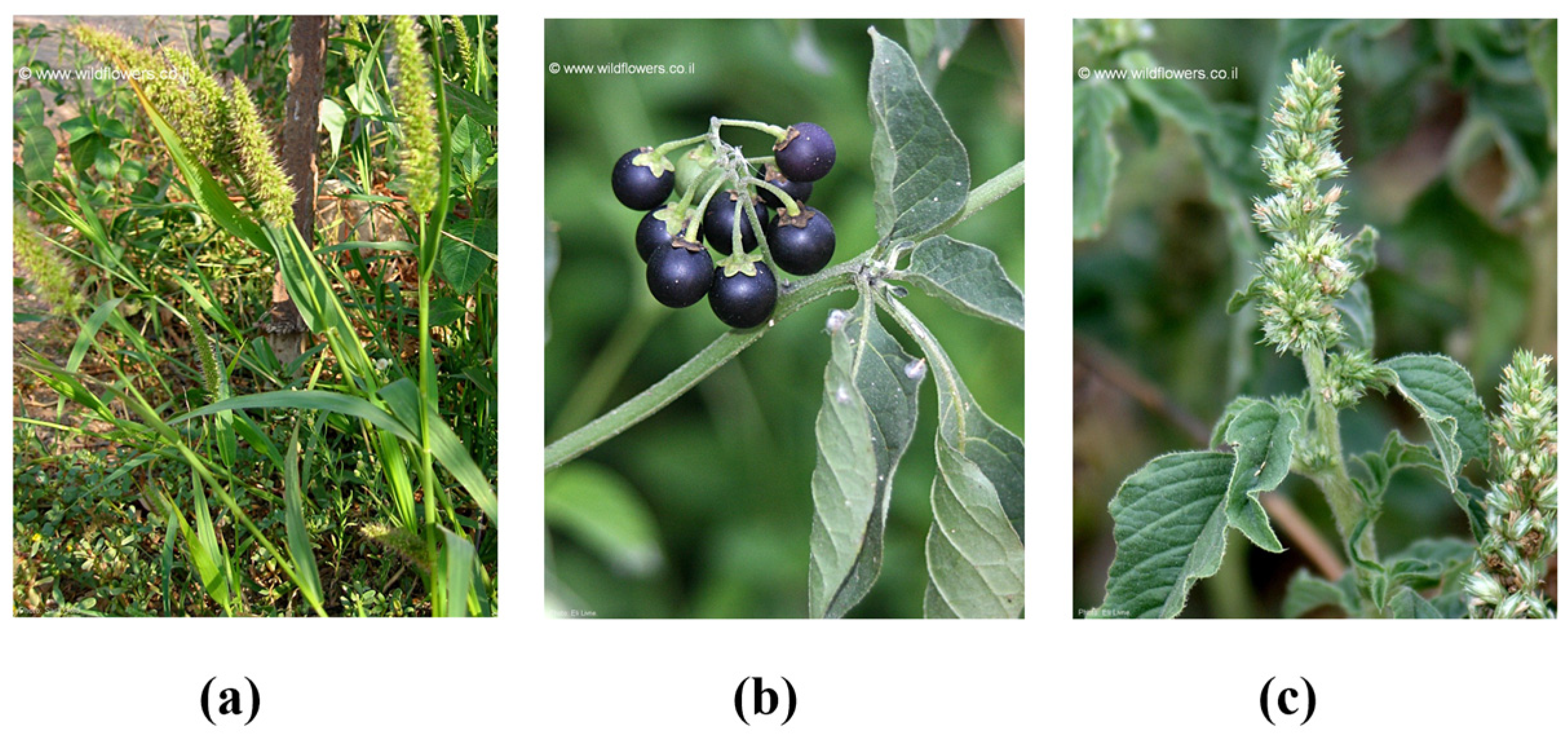
- Species labels: featuring designations for Ar, Sn, Sa, and soil.
- Botanical group labels: including categorizations for monocotyledons (Sa), dicotyledons (Ar, Sn), and soil.
- Photosynthesis mechanisms labels: distinguishing between C3 weeds (Sn) and C4 weeds (Ar, Sa) and soil.
2.2. Experimental Analysis and Evaluation
2.2.1. Feature Selection
Random Forest
Principle Component Analysis (PCA)
2.2.2. Supervised Classification
Support Vector Machine (SVM)
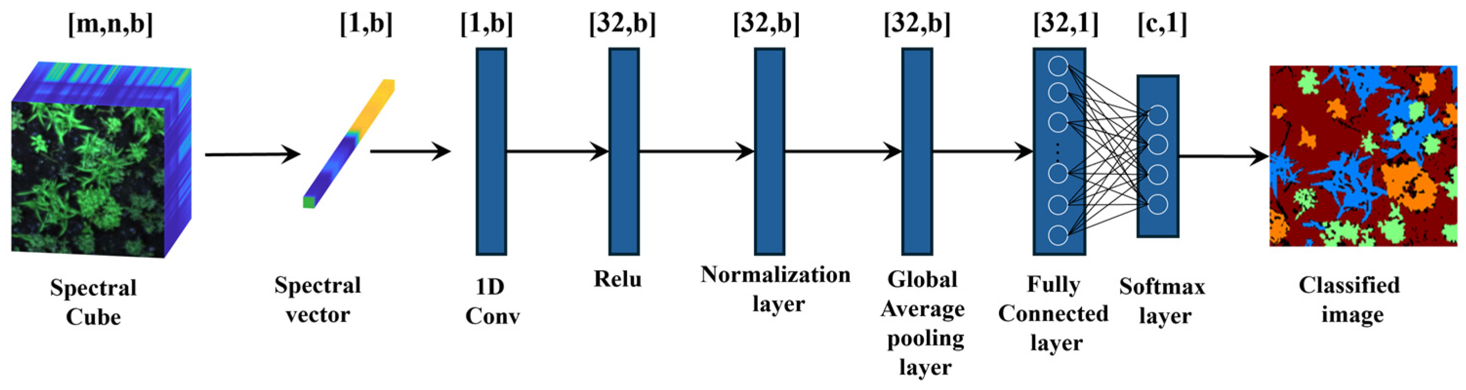
One-Dimensional Convolutional Neural Network
2.2.3. Spectral Unmixing
3. Results
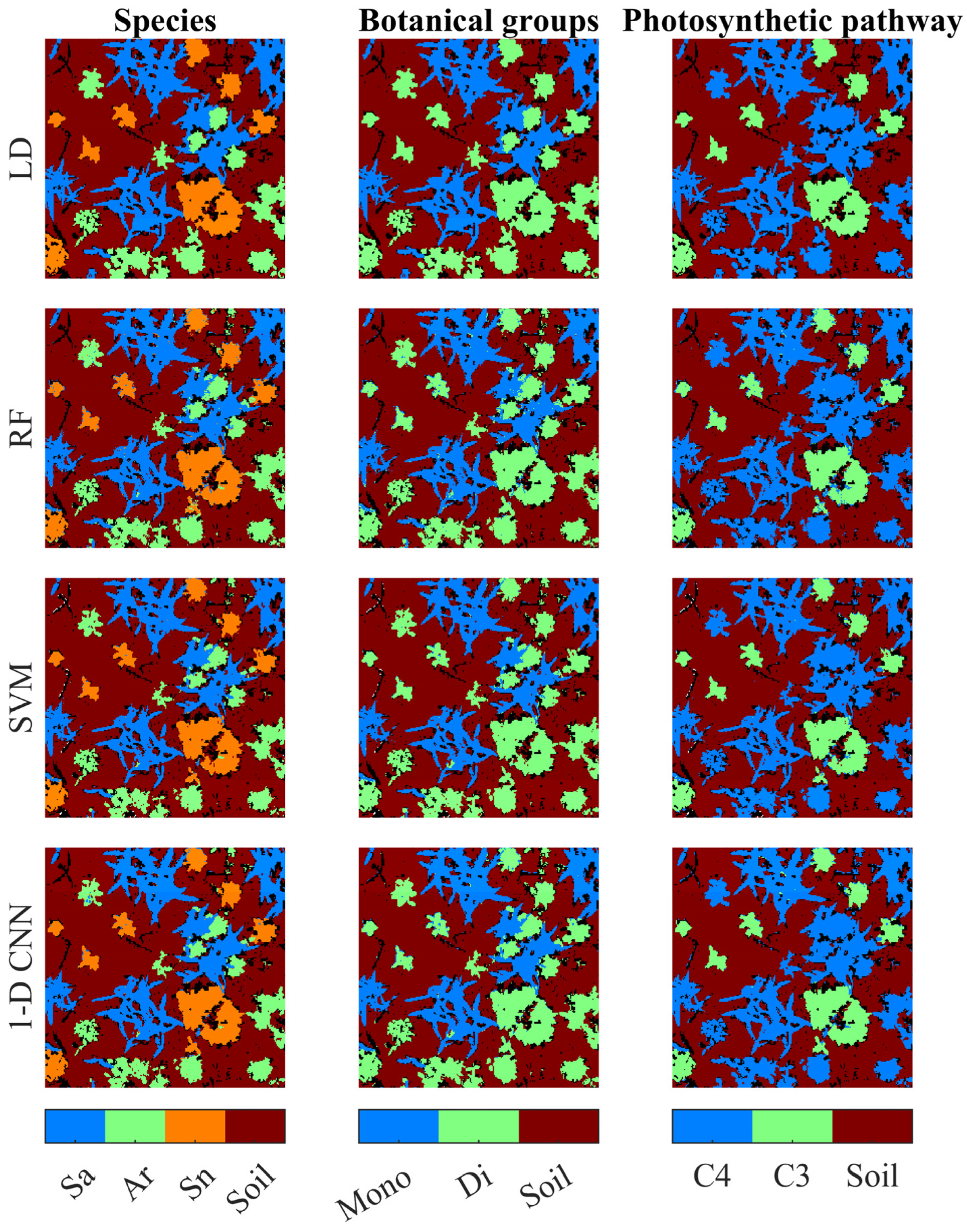
3.1. Classification Based on Full Spectra
3.2. Features Selection and Reduction
3.3. Classification Based on Selected Features
3.4. Spectral Mixture Analysis
4. Discussion
5. Conclusions
6. Data Construction
- A PNG file with an RGB composite image derived from the visible bands in the spectral image.
- A PNG file with the image acquired by the RGB sensor.
- The Capture folder contains the raw data, dark frame, and white reference data cubes.
- The Results folder contains the “.dat” and “.hdr” files of the scene’s reflectance data cube.
- The Label folder contains two sub-folders: the “RGB” folder contains the original labels sampled on the RGB image and the “Hyperspectral” folder contains the transformed labels for the hyperspectral images. Both folders include three image files, with a label assigned for each pixel according to its species, botanical group, and photosynthetic mechanism.
- The root folder includes a README file providing information about the numerical label for each class in the Label files.
Author Contributions
Funding
Data Availability Statement
Conflicts of Interest
References
- Pimentel, D.; Zuniga, R.; Morrison, D. Update on the Environmental and Economic Costs Associated with Alien-Invasive Species in the United States. Ecol. Econ. 2005, 52, 273–288. [Google Scholar] [CrossRef]
- Lati, R.N.; Rasmussen, J.; Andujar, D.; Dorado, J.; Berge, T.W.; Wellhausen, C.; Pflanz, M.; Nordmeyer, H.; Schirrmann, M.; Eizenberg, H.; et al. Site-specific Weed Management—Constraints and Opportunities for the Weed Research Community: Insights from a Workshop. Weed Res. 2021, 61, 147–153. [Google Scholar] [CrossRef]
- Li, Y.; Al-Sarayreh, M.; Irie, K.; Hackell, D.; Bourdot, G.; Reis, M.M.; Ghamkhar, K. Identification of Weeds Based on Hyperspectral Imaging and Machine Learning. Front. Plant Sci. 2021, 11, 611622. [Google Scholar] [CrossRef] [PubMed]
- Buitrago, M.F.; Groen, T.A.; Hecker, C.A.; Skidmore, A.K. Spectroscopic Determination of Leaf Traits Using Infrared Spectra. Int. J. Appl. Earth Obs. Geoinf. 2018, 69, 237–250. [Google Scholar] [CrossRef]
- Ronay, I.; Ephrath, J.E.; Eizenberg, H.; Blumberg, D.G.; Maman, S. Hyperspectral Reflectance and Indices for Characterizing the Dynamics of Crop–Weed Competition for Water. Remote Sens. 2021, 13, 513. [Google Scholar] [CrossRef]
- Hasan, A.S.M.M.; Sohel, F.; Diepeveen, D.; Laga, H.; Jones, M.G.K. A Survey of Deep Learning Techniques for Weed Detection from Images. Comput. Electron. Agric. 2021, 184, 106067. [Google Scholar] [CrossRef]
- Basinger, N.T.; Jennings, K.M.; Hestir, E.L.; Monks, D.W.; Jordan, D.L.; Everman, W.J. Phenology Affects Differentiation of Crop and Weed Species Using Hyperspectral Remote Sensing. Weed Technol. 2020, 34, 897–908. [Google Scholar] [CrossRef]
- Zhang, Y.; Slaughter, D.C. Hyperspectral Species Mapping for Automatic Weed Control in Tomato under Thermal Environmental Stress. Comput. Electron. Agric. 2011, 77, 95–104. [Google Scholar] [CrossRef]
- Persello, C.; Member, S.; Grift, J.; Fan, X.; Paris, C.; Hänsch, R.; Koeva, M.; Nelson, A. AI4SmallFarms: A Dataset for Crop Field Delineation in Southeast Asian Smallholder Farms. IEEE Geosci. Remote Sens. Lett. 2023, 20, 2505705. [Google Scholar] [CrossRef]
- Nascimento, E.; Just, J.; Almeida, J.; Almeida, T. Productive Crop Field Detection: A New Dataset and Deep-Learning Benchmark Results. IEEE Geosci. Remote Sens. Lett. 2023, 20, 5002005. [Google Scholar] [CrossRef]
- Krestenitis, M.; Raptis, E.K.; Kapoutsis, A.C.; Ioannidis, K.; Kosmatopoulos, E.B.; Vrochidis, S.; Kompatsiaris, I. CoFly-WeedDB: A UAV Image Dataset for Weed Detection and Species Identification. Data Brief. 2022, 45, 108575. [Google Scholar] [CrossRef] [PubMed]
- Olsen, A.; Konovalov, D.A.; Philippa, B.; Ridd, P.; Wood, J.C.; Johns, J.; Banks, W.; Girgenti, B.; Kenny, O.; Whinney, J.; et al. DeepWeeds: A Multiclass Weed Species Image Dataset for Deep Learning. Sci. Rep. 2019, 9, 2058. [Google Scholar] [CrossRef] [PubMed]
- Sudars, K.; Jasko, J.; Namatevs, I.; Ozola, L.; Badaukis, N. Dataset of Annotated Food Crops and Weed Images for Robotic Computer Vision Control. Data Brief. 2020, 31, 105833. [Google Scholar] [CrossRef] [PubMed]
- Sa, I.; Chen, Z.; Popovic, M.; Khanna, R.; Liebisch, F.; Nieto, J.; Siegwart, R. WeedNet: Dense Semantic Weed Classification Using Multispectral Images and MAV for Smart Farming. IEEE Robot. Autom. Lett. 2018, 3, 588–595. [Google Scholar] [CrossRef]
- Sa, I.; Popović, M.; Khanna, R.; Chen, Z.; Lottes, P.; Liebisch, F.; Nieto, J.; Stachniss, C.; Walter, A.; Siegwart, R. WeedMap: A Large-Scale Semantic Weed Mapping Framework Using Aerial Multispectral Imaging and Deep Neural Network for Precision Farming. Remote Sens. 2018, 10, 1423. [Google Scholar] [CrossRef]
- Hennessy, A.; Clarke, K.; Lewis, M. Hyperspectral Classification of Plants: A Review of Waveband Selection Generalisability. Remote Sens. 2020, 12, 113. [Google Scholar] [CrossRef]
- Gold, S. (n.d). Setaria adhaerens [Photograph]. Wild Flowers. Available online: https://www.wildflowers.co.il/images/merged/1374-l.jpg?Setaria%20adhaerens (accessed on 24 July 2024).
- Gold, S. (n.d). Solanum nigrum [Photograph]. Wild Flowers. Available online: https://www.wildflowers.co.il/images/merged/190-l-1.jpg?Solanum%20nigrum (accessed on 24 July 2024).
- Livne, E. (n.d). Amaranthus retroflexus [Photograph]. Wild Flowers. Available online: https://www.wildflowers.co.il/images/merged/510-l.jpg?Amaranthus%20retroflexus (accessed on 24 July 2024).
- Meyer, G.E.; Neto, J.C. Verification of Color Vegetation Indices for Automated Crop Imaging Applications. Comput. Electron. Agric. 2008, 63, 282–293. [Google Scholar] [CrossRef]
- Rublee, E.; Rabaud, V.; Konolige, K.; Bradski, G. ORB: An Efficient Alternative to SIFT or SURF. In Proceedings of the IEEE International Conference on Computer Vision, Barcelona, Spain, 6–13 November 2011. [Google Scholar]
- Wang, A.; Zhang, W.; Wei, X. A Review on Weed Detection Using Ground-Based Machine Vision and Image Processing Techniques. Comput. Electron. Agric. 2019, 158, 226–240. [Google Scholar] [CrossRef]
- Ronay, I.; Nisim Lati, R.; Kizel, F. Spectral Mixture Analysis for Weed Traits Identification under Varying Resolutions and Growth Stages. Comput. Electron. Agric. 2024, 220, 108859. [Google Scholar] [CrossRef]
- Kizel, F.; Shoshany, M.; Netanyahu, N.S.; Even-Tzur, G.; Benediktsson, J.A. A Stepwise Analytical Projected Gradient Descent Search for Hyperspectral Unmixing and Its Code Vectorization. IEEE Trans. Geosci. Remote Sens. 2017, 55, 4925–4943. [Google Scholar] [CrossRef]
- Luo, B.; Yang, C.; Chanussot, J.; Zhang, L. Crop Yield Estimation Based on Unsupervised Linear Unmixing of Multidate Hyperspectral Imagery. IEEE Trans. Geosci. Remote Sens. 2013, 51, 162–173. [Google Scholar] [CrossRef]
- Sapkota, B.; Singh, V.; Cope, D.; Valasek, J.; Bagavathiannan, M. Mapping and Estimating Weeds in Cotton Using Unmanned Aerial Systems-Borne Imagery. AgriEngineering 2020, 2, 350–366. [Google Scholar] [CrossRef]
- Machidon, A.L.; Del Frate, F.; Picchiani, M.; Machidon, O.M.; Ogrutan, P.L. Geometrical Approximated Principal Component Analysis for Hyperspectral Image Analysis. Remote Sens. 2020, 12, 1698. [Google Scholar] [CrossRef]
- Gausman, H.W. Plant Leaf Optical Properties in Visible and Near-Infrared Light; International Center for Arid and Semiarid Land Studies (ICASALS): Lubbock, TX, USA, 1985. [Google Scholar]
- Liu, L.; Cheng, Z. Mapping C3 and C4 Plant Functional Types Using Separated Solar-Induced Chlorophyll Fluorescence from Hyperspectral Data. Int. J. Remote Sens. 2011, 32, 9171–9183. [Google Scholar] [CrossRef]
- Adjorlolo, C.; Mutanga, O.; Cho, M.A.; Ismail, R. Spectral Resampling Based on User-Defined Inter-Band Correlation Filter: C3 and C4 Grass Species Classification. Int. J. Appl. Earth Obs. Geoinf. 2013, 21, 535–544. [Google Scholar] [CrossRef]
- Chang, G.J.; Oh, Y.; Goldshleger, N.; Shoshany, M. Biomass Estimation of Crops and Natural Shrubs by Combining Red-Edge Ratio with Normalized Difference Vegetation Index. J. Appl. Remote Sens. 2022, 16, 014501. [Google Scholar] [CrossRef]
- Kizel, F. Resolution Enhancement of Unsupervised Classification Maps Through Data Fusion of Spectral and Visible Images from Different Sensing Instruments. In Proceedings of the 2021 IEEE International Geoscience and Remote Sensing Symposium IGARSS, Brussels, Belgium, 11–16 July 2021. [Google Scholar]
- Kizel, F.; Benediktsson, J.A. Spatially Enhanced Spectral Unmixing Through Data Fusion of Spectral and Visible Images from Different Sensors. Remote Sens. 2020, 12, 1255. [Google Scholar] [CrossRef]


| DAS | Sa | Ar | Sn | Monocots | Dicots | C3 | C4 | Soil |
|---|---|---|---|---|---|---|---|---|
| 7 | 21,218 | 13,290 | 6321 | 21,218 | 19,611 | 34,508 | 6321 | 372,700 |
| 8 | 38,351 | 24,578 | 14,730 | 38,351 | 39,308 | 62,929 | 14,730 | 267,935 |
| 9 | 45,008 | 30,893 | 18,686 | 45,008 | 49,579 | 75,901 | 18,686 | 374,651 |
| 12 | 67,132 | 44,083 | 31,935 | 67,132 | 76,018 | 111,215 | 31,935 | 386,183 |
| 13 | 79,511 | 56,523 | 44,939 | 79,511 | 101,462 | 136,034 | 44,939 | 342,641 |
| 14 | 87,074 | 57,529 | 50,612 | 87,074 | 108,141 | 144,603 | 50,612 | 323,484 |
| SVM | 1D-CNN | ||||||||||
|---|---|---|---|---|---|---|---|---|---|---|---|
| DAS | Full Spectra | VIS | NIR | VIS + NIR | PCA | Full Spectra | VIS | NIR | VIS + NIR | PCA | |
| Species | 7 | 0.96 | 0.96 | 0.94 | 0.97 | 0.97 | 0.96 | 0.96 | 0.94 | 0.96 | 0.97 |
| 8 | 0.93 | 0.89 | 0.85 | 0.92 | 0.92 | 0.92 | 0.89 | 0.85 | 0.92 | 0.93 | |
| 9 | 0.93 | 0.91 | 0.87 | 0.94 | 0.94 | 0.93 | 0.91 | 0.87 | 0.94 | 0.95 | |
| 12 | 0.89 | 0.83 | 0.82 | 0.90 | 0.90 | 0.92 | 0.85 | 0.83 | 0.92 | 0.92 | |
| 13 | 0.88 | 0.83 | 0.78 | 0.91 | 0.91 | 0.92 | 0.84 | 0.79 | 0.91 | 0.91 | |
| 14 | 0.88 | 0.80 | 0.78 | 0.90 | 0.90 | 0.90 | 0.81 | 0.80 | 0.90 | 0.91 | |
| Botanical groups | 7 | 0.96 | 0.96 | 0.95 | 0.97 | 0.97 | 0.97 | 0.96 | 0.94 | 0.97 | 0.98 |
| 8 | 0.94 | 0.89 | 0.87 | 0.93 | 0.93 | 0.93 | 0.90 | 0.87 | 0.93 | 0.94 | |
| 9 | 0.93 | 0.91 | 0.89 | 0.95 | 0.95 | 0.95 | 0.91 | 0.89 | 0.95 | 0.95 | |
| 12 | 0.90 | 0.85 | 0.85 | 0.92 | 0.92 | 0.93 | 0.86 | 0.85 | 0.93 | 0.93 | |
| 13 | 0.89 | 0.85 | 0.84 | 0.92 | 0.92 | 0.92 | 0.85 | 0.84 | 0.92 | 0.92 | |
| 14 | 0.89 | 0.82 | 0.83 | 0.91 | 0.92 | 0.92 | 0.82 | 0.83 | 0.91 | 0.92 | |
| Photosynthetic pathway | 7 | 0.96 | 0.96 | 0.97 | 0.97 | 0.97 | 0.97 | 0.96 | 0.97 | 0.97 | 0.97 |
| 8 | 0.93 | 0.90 | 0.91 | 0.91 | 0.91 | 0.91 | 0.91 | 0.91 | 0.92 | 0.94 | |
| 9 | 0.93 | 0.92 | 0.93 | 0.93 | 0.93 | 0.93 | 0.92 | 0.93 | 0.93 | 0.95 | |
| 12 | 0.89 | 0.87 | 0.89 | 0.90 | 0.89 | 0.92 | 0.87 | 0.89 | 0.92 | 0.93 | |
| 13 | 0.90 | 0.87 | 0.87 | 0.91 | 0.92 | 0.93 | 0.87 | 0.87 | 0.92 | 0.93 | |
| 14 | 0.89 | 0.84 | 0.86 | 0.90 | 0.91 | 0.92 | 0.85 | 0.87 | 0.91 | 0.92 | |
| Precision | Recall | |||||||||||
|---|---|---|---|---|---|---|---|---|---|---|---|---|
| Trait | Method | Class | Full Spectra | VIS | NIR | VIS + NIR | PCA | Full Spectra | VIS | NIR | VIS + NIR | PCA |
| Species | CNN | Sa | 85.5 | 54 | 51.8 | 81.8 | 85.5 | 82.7 | 83.4 | 70.8 | 86.4 | 85.1 |
| Ar | 83.9 | 69.7 | 51.9 | 80.3 | 79 | 71.4 | 65.8 | 21.1 | 76.1 | 81.2 | ||
| Sn | 87.8 | 26.7 | 61.4 | 83 | 87.8 | 74.4 | 0 | 48.1 | 73.9 | 72.4 | ||
| Soil | 92.5 | 94.1 | 93.4 | 95 | 94.7 | 97.9 | 95.9 | 97.3 | 96.1 | 97 | ||
| SVM | Sa | 89.3 | 53.4 | 48 | 84 | 83.5 | 79 | 86.1 | 84.2 | 84.9 | 84.7 | |
| Ar | 83.8 | 76 | 100 | 81.3 | 81.4 | 74.9 | 52.9 | 5 | 76.9 | 78.6 | ||
| Sn | 91.6 | 100 | 70.6 | 88.5 | 88.5 | 69.2 | 5 | 44 | 69.3 | 69.3 | ||
| Soil | 90.6 | 93.2 | 94.6 | 93.7 | 94.1 | 98.6 | 96.7 | 96.9 | 97.5 | 97.5 | ||
| Botanical groups | CNN | Mono | 86.3 | 60.6 | 62.6 | 83.3 | 86.1 | 83.8 | 62.7 | 33.4 | 84 | 84.1 |
| Di | 88.9 | 67.9 | 60.9 | 87.3 | 88.9 | 85.1 | 56.3 | 80.5 | 83.8 | 85.3 | ||
| Soil | 94.7 | 93.1 | 94.7 | 94.9 | 95 | 96.8 | 96.4 | 96.4 | 96 | 96.9 | ||
| SVM | Mono | 90.2 | 58.4 | 64.4 | 85.4 | 86.2 | 78.5 | 63.1 | 49.8 | 83.8 | 82.9 | |
| Di | 91.6 | 66.1 | 68.1 | 89.3 | 89.6 | 81.3 | 57.6 | 73.3 | 83.1 | 84.1 | ||
| Soil | 91.7 | 93.6 | 94 | 94.4 | 94.5 | 98.4 | 96.8 | 97.3 | 97 | 97.4 | ||
| Photosynthetic pathways | CNN | C4 | 87.2 | 67.4 | 73 | 84.5 | 85.9 | 88.9 | 90.4 | 87.2 | 89.3 | 88.6 |
| C3 | 89.3 | 100 | 67.9 | 85.4 | 85.7 | 74.3 | 0 | 20.6 | 69.6 | 73.8 | ||
| Soil | 95 | 91.8 | 94.5 | 95.4 | 95.5 | 96.7 | 95.2 | 96.6 | 95.8 | 96.3 | ||
| SVM | C4 | 89.5 | 68.9 | 72.4 | 81.7 | 83 | 84.5 | 89.8 | 90.7 | 89.6 | 89.5 | |
| C3 | 92.9 | 100 | 95.6 | 92.4 | 92.8 | 67.6 | 5 | 14.6 | 53.8 | 59.4 | ||
| Soil | 92.1 | 91.5 | 94.9 | 94.8 | 95 | 98.4 | 95.8 | 96.7 | 96.9 | 97 | ||
| EM | Full Spectra | VIS | NIR | VIS + NIR | PCA | |
|---|---|---|---|---|---|---|
| Species | Sa | 10.92 | 8.60 | 9.45 | 7.71 | 10.91 |
| Ar | 6.76 | 5.86 | 6.85 | 6.35 | 10.74 | |
| Sn | 7.82 | 8.71 | 5.64 | 4.58 | 6.34 | |
| Soil | 4.58 | 4.50 | 6.35 | 8.17 | 6.06 | |
| Botanical groups | Mono | 6.75 | 7.83 | 9.83 | 7.46 | 9.43 |
| Dicot | 6.81 | 11.84 | 9.95 | 7.25 | 8.78 | |
| Soil | 3.96 | 6.15 | 7.71 | 10.43 | 6.02 | |
| Photosynthetic pathway | C4 | 12.10 | 17.89 | 9.61 | 11.17 | 10.40 |
| C3 | 9.52 | 13.16 | 5.71 | 5.54 | 6.98 | |
| Soil | 4.52 | 6.32 | 6.29 | 9.45 | 6.08 |
| DAS | Sa | Ar | Sn | Soil | Monocots | Dicots | Soil | C4 | C3 | Soil |
|---|---|---|---|---|---|---|---|---|---|---|
| 7 | 2.01 | 2.30 | 3.76 | 3.70 | 2.09 | 2.98 | 3.09 | 3.49 | 4.59 | 3.82 |
| 8 | 5.19 | 3.30 | 7.13 | 4.52 | 3.33 | 4.59 | 4.37 | 7.60 | 8.38 | 4.56 |
| 9 | 3.90 | 2.93 | 5.50 | 4.12 | 3.54 | 3.61 | 3.66 | 6.60 | 6.55 | 3.73 |
| 12 | 8.79 | 5.57 | 7.83 | 4.38 | 6.57 | 6.48 | 4.35 | 10.51 | 10.47 | 4.67 |
| 13 | 12.33 | 7.16 | 9.23 | 7.15 | 8.89 | 7.69 | 6.81 | 14.64 | 10.33 | 7.07 |
| 14 | 10.92 | 6.76 | 7.82 | 4.58 | 6.75 | 6.81 | 3.96 | 12.10 | 9.52 | 4.52 |
Disclaimer/Publisher’s Note: The statements, opinions and data contained in all publications are solely those of the individual author(s) and contributor(s) and not of MDPI and/or the editor(s). MDPI and/or the editor(s) disclaim responsibility for any injury to people or property resulting from any ideas, methods, instructions or products referred to in the content. |
© 2024 by the authors. Licensee MDPI, Basel, Switzerland. This article is an open access article distributed under the terms and conditions of the Creative Commons Attribution (CC BY) license (https://creativecommons.org/licenses/by/4.0/).
Share and Cite
Ronay, I.; Lati, R.N.; Kizel, F. Weed Species Identification: Acquisition, Feature Analysis, and Evaluation of a Hyperspectral and RGB Dataset with Labeled Data. Remote Sens. 2024, 16, 2808. https://doi.org/10.3390/rs16152808
Ronay I, Lati RN, Kizel F. Weed Species Identification: Acquisition, Feature Analysis, and Evaluation of a Hyperspectral and RGB Dataset with Labeled Data. Remote Sensing. 2024; 16(15):2808. https://doi.org/10.3390/rs16152808
Chicago/Turabian StyleRonay, Inbal, Ran Nisim Lati, and Fadi Kizel. 2024. "Weed Species Identification: Acquisition, Feature Analysis, and Evaluation of a Hyperspectral and RGB Dataset with Labeled Data" Remote Sensing 16, no. 15: 2808. https://doi.org/10.3390/rs16152808
APA StyleRonay, I., Lati, R. N., & Kizel, F. (2024). Weed Species Identification: Acquisition, Feature Analysis, and Evaluation of a Hyperspectral and RGB Dataset with Labeled Data. Remote Sensing, 16(15), 2808. https://doi.org/10.3390/rs16152808