Abstract
The study of the polarimetric target decomposition algorithm with physical scattering models has contributed to the development of the field of remote sensing because of its simple and clear physical meaning with a small computational effort. However, most of the volume scattering models in these algorithms are for forests or crops, and there is a lack of volume scattering models for grasslands. In order to improve the accuracy of the polarimetric target decomposition algorithm adapted to grassland data, in this paper, a novel volume scattering model is derived considering the characteristics of real grassland plant structure and combined with the backward scattering coefficients of grass, which is abstracted as a rotatable ellipsoid of variable shape. In the process of rotation, the possibility of rotation is considered in two dimensions, the tilt angle and canting angle; for particle shape, the anisotropy degree A is directly introduced as a parameter to describe and expand the applicability of the model at the same time. After obtaining the analytical solution of the parameters and using the principle of least negative power to determine the optimal solution of the model, the algorithm is validated by applying it to the C-band AirBorne dataset of Hunshandak grassland in Inner Mongolia and the X-band Cosmos-Skymed dataset of Xiwuqi grassland in Inner Mongolia. The performance of the algorithm with five polarimetric target decomposition algorithms is studied comparatively. The experimental results show that the algorithm proposed in this paper outperforms the other algorithms in terms of grassland decomposition accuracy on different bands of data.
1. Introduction
Grassland ecosystems have ecological functions such as windbreak and sand fixation, water conservation, etc., which is an important part of the natural ecosystem and has important geographic value for maintaining ecological balance, regional economy, and human history [1]. However, neglecting the geographic location and interannual variation of spring phenology leads to a high risk of overgrazing and grassland degradation, which is a problem that needs to be solved urgently [2]. Therefore, it is important to monitor grasslands. In recent years, there has been increasing interest in the potential offered by microwave satellite-based instruments. This microwave technique measures the strength of backscattered signals from the surface in almost all weather and lighting conditions [3]. The backscatter signal from vegetated surfaces is a function of the soil surface, the radar system and the biophysical parameters of the scatterers in the vegetation that can influence the depth to which the radar wave penetrates. Interpreting the backscatter signal gives us the parameters we want. This is one of the features that distinguishes the microwave technique from optical satellites. The Polarimetric Synthetic Aperture Radar (SAR) with full polarization measurement capability has become a mainstream sensor in the fields of earth observation, disaster remote sensing, ocean remote sensing, reconnaissance and surveillance, etc., and has become more and more widely used [4]. The polarimetric target decomposition algorithm is the main implementation method for polarimetric feature extraction of polarimetric SAR images [5]. Currently, polarimetric target decomposition theory is divided into two categories: coherent target decomposition for describing pure targets and incoherent target decomposition for describing distributed targets [6]. Since distributed targets are more widespread in nature, the methods of incoherent polarimetric target decomposition have been more widely used. Decomposition of incoherent targets was first proposed by Huynen [7], which is divided into two main categories: eigenvalue incoherent polarimetric target decomposition [8,9,10,11] and model-based incoherent polarimetric target decomposition [12,13,14]. The basic decomposition framework used in this paper is the model-based incoherent t polarimetric target decomposition algorithm. The algorithms of Freeman [12] and Yamaguchi [14] are the classical algorithms for model-based polarimetric target decomposition. This type of algorithm is not based entirely on mathematical means, but makes full use of the scattering properties of radars, and the decomposed scattering model and parameters have a clear physical meaning. Therefore, this type of method has the advantage of clear physical meaning with less computation and has higher practical value [15,16,17].
However, the model-based polarimetric target decomposition algorithm has the following two problems: (1) the problem of inadequate application of polarization data due to the reflection symmetry assumption; (2) the problem of negative power due to the discrepancy between the scattering model and the observation target. A large number of improvements have been made by domestic and foreign scholars to address the above problems. Adding scattering components is one of the most common methods to solve the first problem. In 2005, Yamaguchi et al. [14] introduced spiral scattering components to break the reflection symmetry assumption. In 2018, Gulab and Yamaguchi [18] proposed a six-component decomposition method with the addition of oriented dipoles scattering and composite scattering matrices that utilize the component of the polarization coherency matrix. In 2019, Gulab [19] built upon the above study by adding matrices corresponding to the real part of while removing the oriented-angle compensation as an operation. This seven-component decomposition utilizes seven of the nine independent parameters. In addition to increasing the scattering components to account for the corresponding independent parameters, reducing the number of independent parameters can also improve the parameter utilization. Because the undulation of the terrain and the tilted arrangement of the buildings cause a shift in the polarization azimuth, orientation angle compensation is used to minimize the cross-polarization component by rotating the polarization coherency matrix so that the real part of is zero after the rotation. Because serves as the main source of the volume scattering model in the classical polarimetric target decomposition algorithm, the orientation angle compensation minimizes the cross-polarization term and also alleviates the problem of volume scattering overestimation to some extent. Orientation angle compensation has been used as a preprocessing step for the polarimetric coherency matrix, and the algorithms that introduce this processing [20,21,22] have improved. In 2012, Yamaguchi [23] proposed an algorithm to perform a double unitary transformation on the polarimetric coherency matrix, which completely eliminates the elements and reduces the nine independent parameters to seven, as well as greatly alleviates the negative power problem. However, the above two approaches usually introduce models that cannot correspond explicitly to the actual observation targets, making the advantages of the model-based decomposition methods not obvious enough. Hongzhong Li [24] and Wentao An [25], on the other hand, optimized the algorithms by directly correcting the reflection symmetry assumption.
For the second problem, scholars have proposed solutions from several perspectives. In 2011, van Zyl et al. [26] introduced a non-negative eigenvalue constraint criterion to effectively avoid the negative power phenomenon while retaining the traditional model. Combining the advantages of eigenvalue-based decomposition, hybrid decomposition can also avoid negative power. Cloude [27] proposed a hybrid Freeman/eigenvalue decomposition method in which the surface scattering is orthogonal to the double bounce scattering. In 2014, Yi Cui et al. [28] combined the two, which strictly guarantees that all decompositions are non-negative and fully utilizes the polarimetric information. In 2016, Zou Bin et al. [29] improved the negative power problem by combining the eigen decomposition with the four-component decomposition. Maurya [30] proposed a hybrid technique for the decomposition of polarimetric synthetic aperture radar (SAR) data with the aim of solving the negative power problem encountered in model-based decomposition methods. While the Freeman decomposition assumes that the probability density function associated with the orientation angle of the elementary scatterer satisfies a uniform distribution, Yamaguchi proposed a truncated sinusoidal probability distribution to replace the uniform distribution, which makes the volume scattering model more accurate and also suggests an idea for other scholars to improve the volume scattering model.
Neumann et al. [31] proposed the use of von Mises distribution to characterize the canopy of vegetation. Arii et al. [32] introduced a probability distribution of nth cosine squared function. This distribution is mainly described by the orientation angle mean and surface roughness parameters. In addition, based on the distribution function of the phase difference in multiview data, Lee et al. [33] proposed a series of models for matching different azimuthal distributions. Compared with the improvement of volume scattering models, the improvement of surface scattering models and double bounce scattering models are less studied, but they are also an idea for optimization algorithms.
In 2014, Chen Siwei et al. [34] refined the scattering model by introducing a rotation angle parameter to rotate the traditional surface scattering model and double bounce scattering models. To make the volume scattering model more compatible with the observation target, the volume scattering model can also be extended by introducing adaptive parameters, and the volume scattering model can be made more compatible with the observation target by automatically adjusting the volume scattering model through the observation values. In 2010, Arii et al. [35] introduced the random direction angle and random degree adaptive parameters to extend the volume scattering model without the reflection symmetry assumption. In 2011, Antropov et al. [36] proposed a generalized model for the contribution of forest volume scattering, which extends the volume scattering range. Huang et al. [37] used an improved volume scattering model based on the nth cosine function to describe vegetation, where the parameters are determined by the optimal values from multiple experiments. Wang et al. [38] introduced parameters to reduce the negative power by modeling dipole aggregation. Wang T et al. [39] proposed a full parameter optimization method based on the residual matrix, which will consider all the elements of the coherency matrix to achieve priority-free optimization. In order to improve the accuracy of the decomposition, proposing a specific model for a specific observation target is also a way to solve the problem. Chen et al. [40] combined the polarization orientation (PO) in the four-component decomposition, and used this method to study the extent of tsunami damages to the structures in urban areas, which is of great significance in the assessment of natural disasters. Zhang et al. [41] investigated the characteristics of the edge region of the building after introducing line scattering, which decomposes the covariance matrix into a weighted sum of five basic scattering mechanisms, namely surface scattering, double bounce scattering, volume scattering, helical scattering, and line scattering, to construct a more generalized scattering model, which obtains better results in man-made target detection. Xiang et al. [42] used a rotating double bounce model to effectively separate the building-oriented induced cross-scattering from the overall high-pressure component. Dou et al. [15] combined a generalized volume scattering model with a simplified adaptive volume scattering model and a simplified Neumann volume scattering model to successfully separate the surface and the above-ground vegetation by using the two-component decomposition as the basic framework, and estimated the soil moisture using the decomposition parameters. Hajnsek et al. [43] used the above three polarized characteristic parameters to distinguish the inversion of surface roughness and soil moisture, which can be estimated separately, thus improving the accuracy of the inversion of surface parameters. Numerous scholars have improved the model-based target decomposition method and achieved better results, which also shows that the model-based target decomposition algorithm has great potential in the field of remote sensing. However, there are fewer volume scattering models proposed for grassland in the current research, which leads to unsatisfactory decomposition results for grassland. Therefore, this paper proposes a novel polarimetric target decomposition algorithm applied to grasslands.
In this paper, an adaptive polarimetric target decomposition algorithm is proposed by taking two-component decomposition as the basic decomposition framework and introducing an adaptive parameter, anisotropy degree (A). In this paper, the particle shape is considered from two dimensions, orientation randomness, i.e., the arrangement direction of the particles, and anisotropy, i.e., the shape of the particles. When considering the orientation randomness of the particles, the spin angle of the grass is ignored in combination with the characteristics of the grass, and the tilt angle is restricted so that the range of its value is no longer allowed to be an arbitrary angle. The anisotropy of the particles is then modeled by the anisotropy degree A, which is used as an adaptive parameter introduced in the text. Such a model is more realistic and the simulation of the grass will be more accurate. After obtaining the analytical solutions of the parameters, the optimal solutions of the parameters are determined by combining the principle of least negative power. Using the proposed decomposition framework, the C-band AirBorne dataset from Hunshandak Grassland in Inner Mongolia and the X-band Cosmos-Skymed dataset from Xiwuqi in Inner Mongolia are used as experimental data to verify the effectiveness of the algorithm.
2. Methodology
2.1. Orientation Angle Compensation
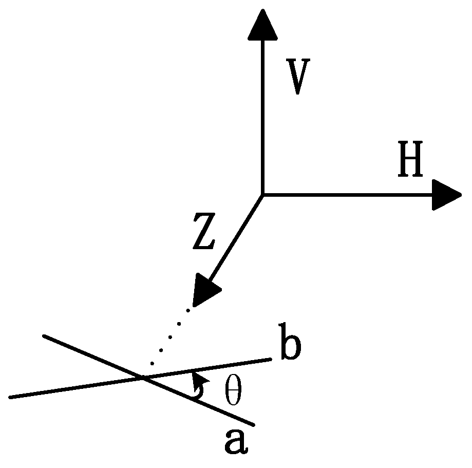
The concept of the orientation angle was first introduced by Huynen in the target decomposition of the matrix [7]. Each pixel point of the target in a polarimetric SAR image has its own orientation angle, and the deorientation operation is precisely designed to eliminate the effects of these randomly distributed orientation angles. It is known that a target shown in Figure 1 has a measured scattering matrix of when in position parallel to the H-axis. By using the Z-axis as the radar line-of-sight direction, the target is rotated counterclockwise by the angle around the radar incidence direction in a plane perpendicular to the radar’s line of sight to reach position b, which is where the angle of orientation comes from.

Figure 1.
Orientation angle rotation.
In order to find the scattering matrix after the target is rotated, this case can be equated to the target not moving; the radar is rotated clockwise by an angle , i.e., the coordinate system HV is rotated clockwise by the angle . Then, the incident electromagnetic wave and the scattered electromagnetic wave become a new coordinate system, as shown below [44]:
where represents the scattering matrix after the target is rotated to position b. The scattering matrix before and after the rotation are related as follows:
From this, the following formula for the deorientation angle of the coherent matrix can be derived [44]:
After determining the orientation angle compensation formula, the most important thing is to determine the value of the rotation angle . Since the component of the coherency matrix consists only of the cross-polarization term, we try to minimize it as much as possible, which is also helpful for the subsequent negative power analysis. The term in Equation (3) can be written as follows:
This gives the derivative of with respect to as follows:
In order to obtain its minimum value, making the derivative zero, i.e., , the following equations can be obtained:
It can be found that remains unchanged while becomes purely imaginary, which exactly fits the spiral scattering model of Yamaguchi’s four-component decomposition. It can also be found that decreases by and increases by the same amount by rotation [20].
2.2. Adaptive Volume Scattering Model
In this paper, an anisotropic particle cloud is chosen to model the scattering properties of grass. The matrices needed for the subsequent algorithms are proposed based on the scattering mechanism. Since the coherency matrix formulation is closer to the physical scattering properties and more zeros appear in the scattering model, all subsequent decompositions in this paper use the coherency matrix [33].
Since the size of grass is much smaller than the wavelength of an electromagnetic wave, we use the concept of polarizability to discuss the scattering mechanism of particles. When a particle is placed into a uniform incident field, that incident field will produce an induced dipole moment as shown below [45]:
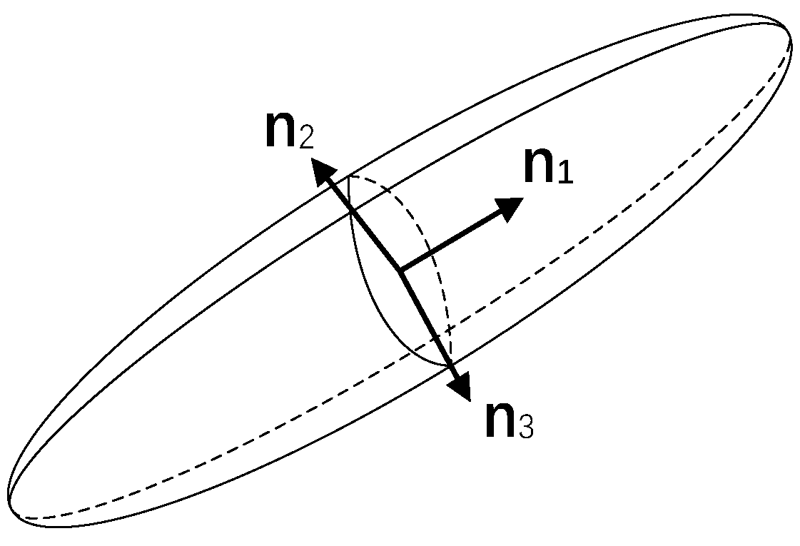
where is the tensor. Thus, the directions of and coincide only when the field is applied to one of the three principal directions of the particle. Let the orientation of the particle in space be characterized by three perpendicular unit vectors , and , as shown in Figure 2.
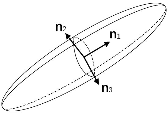
Figure 2.
Three main directions of the particle.
The incident field can thus be expressed as follows:
The particle is then characterized by three tensor components , and , also known as polarizabilities, such that the dipole moment can be expressed as follows:
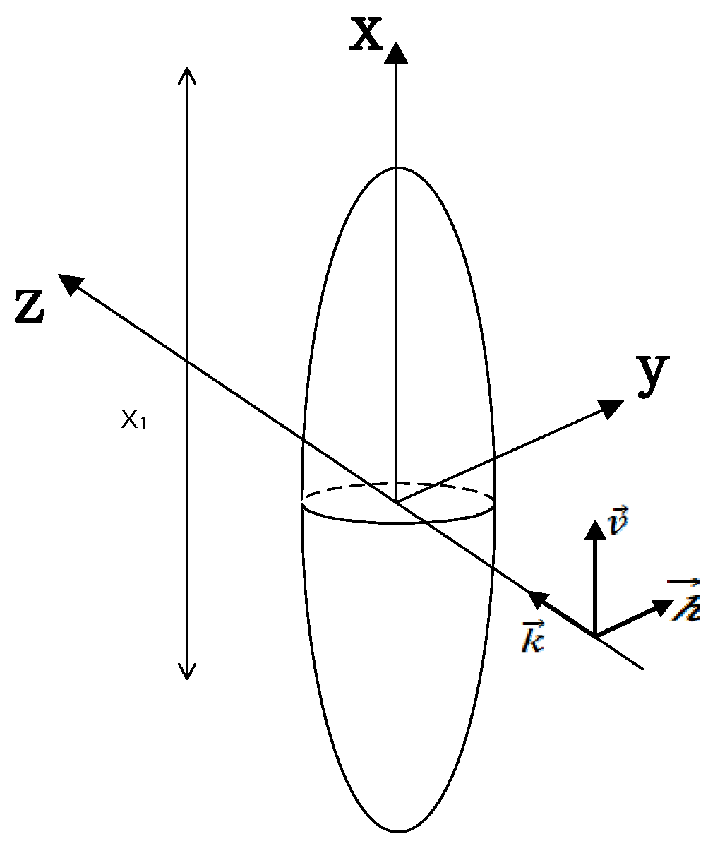
Due to its flexibility in modeling, there are many possible particle shapes with axis lengths only (sphere, needle, disk, etc.); here, we chose the ellipsoid [46]. To compute the scattering matrix for an arbitrary ellipsoid, we place the ellipsoid into a Cartesian coordinate system. For simplicity, the incidence direction is chosen to be the positive Z-axis and only the backscattering case is considered below. Figure 3 shows the ellipsoid in its standard position, i.e., its three axes (, , and ) are parallel to the Cartesian unit vectors x, y, and z, respectively.
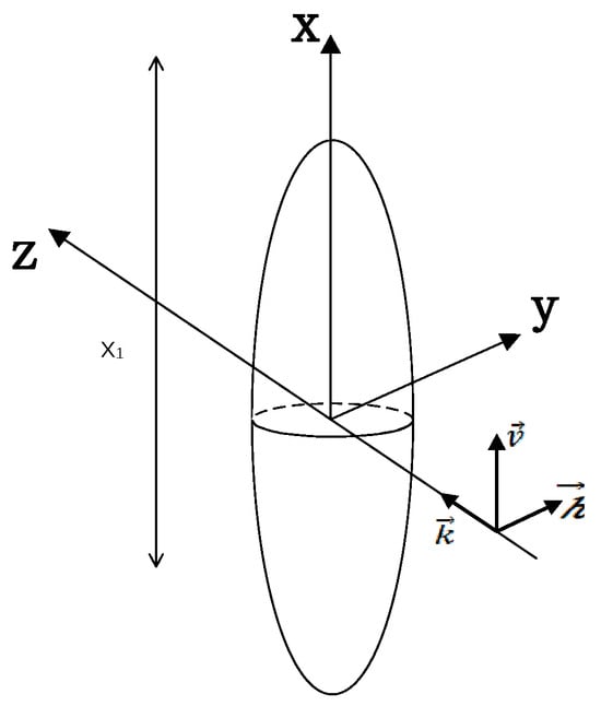
Figure 3.
Standard position ellipsoid.
Induced dipole moments in the direction of the three axes are represented in the Cartesian coordinate system as shown below:
where the incident field is divided into vertical incidence and horizontal incidence .
where then shows the relationship between the Cartesian coordinate system and the three axes of the ellipsoid, as shown below:
A three-dimensional cubic ellipsoid is rotatable in three directions, which are referred to as the rotation angle , the tilt angle , and the canting angle . Changes induced by rotations around a fixed point can be represented by a rotation matrix [45], i.e., we can start by considering rotations in one direction, and the final result can be represented by a matrix product. By assuming a right-handed coordinate system and using the Z-axis as the radar line-of-sight direction, the particle is at the standard position ( = 0°, = 90°). The rotation is shown in Figure 4, where the primitive axes are denoted x, y, and z. Typical rotations around the three directions are denoted as follows:
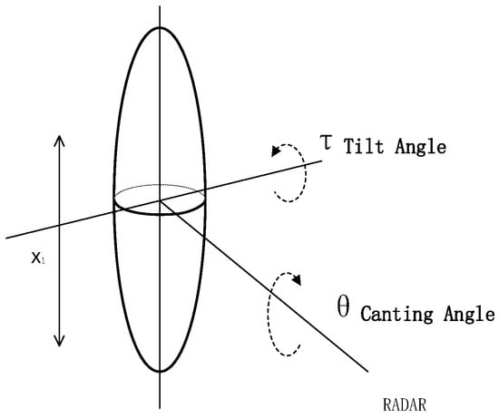
Figure 4.
Schematic of particle rotation. The particle is shown at orientation = 0°, = 90°.
Then, its total rotation can be expressed by its product, as shown below:
It is important to note that in connection with the actual situation, the rotation of the grass is meaningless; therefore, for the particle, the rotation angle here is meaningless, i.e., .
The backscattered field can be obtained as the component perpendicular to the propagation direction [45]. Combined with the backscattering coordinate system, the scattering matrix of the ellipsoid can be derived as follows:
where
The definition of A is below:
In order to reduce the parameters of the model and decrease the complexity of the subsequent decomposition, we perform some parametric simplifications [47]. The spin angle is unobjectionable for the goal of our study, , i.e., for our hypothetical ellipsoid. Furthermore, we are more concerned with the shape of the particles than their specific size; therefore, we consider the relative ratios, such that and .
At this point, substituting the assumptions about the parameters gives the following:
According to the conversion relation between the scattering matrix and the polarimetric coherency matrix, the following expression can be obtained:
where denotes the overall average.
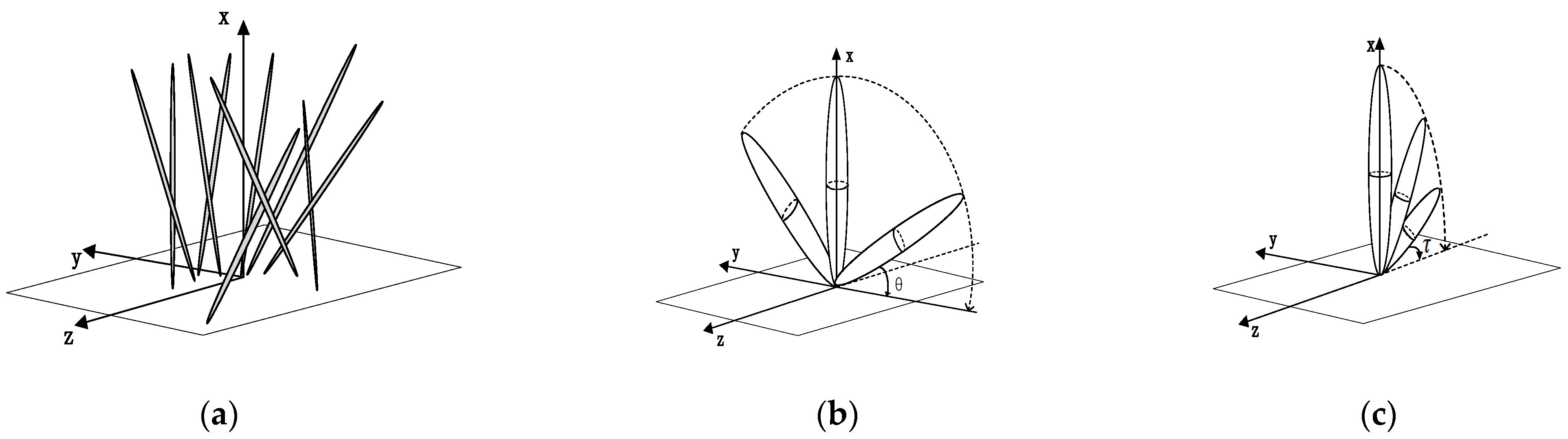
It is assumed that only single scattering is important and that each particle in the cloud is independent of the other particles around it [48]. In this paper, we focus on two main parameters of the particles: the shape and the orientation distribution of the particles, where the shape of the particle is represented by the anisotropy degree A. For the direction distribution of particles, we no longer choose a completely random model, but limit it according to the actual situation. The actual situation of the grassland can be abstracted as shown in Figure 5.

Figure 5.
Abstractions of the actual situation in the meadow. (a) Actual abstraction; (b) effect on the canting angle ; (c) effect on the tilt angle .
From Figure 5a, it can be seen that the rotation angle, the tilt angle and the canting angle are not uniformly distributed within . The rotation angle is not emphasized in this paper to make it zero, and the reason has been explained in the previous section. In reality, the grass growth is not vertically upward, and the bending growth of grass is a factor that must be considered for modeling. In this paper, the degree of incline of grass is characterized in terms of two dimensions: the tilt angle and canting angle. Different degrees of grass incline have different effects on its tilt and canting angles. Figure 5b shows the effect on the canting angle , where different degrees of incline differ only in direction and the particle shape does not change. Figure 5c shows the effect on the tilt angle ; as the grass is tilted, the shape of the particles follows. Therefore, in this paper, considering the particle shape of grass from two dimensions can better fit the actual situation. Combined with the particle rotation schematic in Figure 4, the tilt angleshould be within the range, while the canting angle should be within the range . Therefore, the overall average of the coherency matrix is defined as follows:
According to Equations (25)–(27), the polarimetric coherency matrix of the ellipsoidal particle is obtained by calculation as follows:
2.3. Polarimetric Target Decomposition Algorithm
The scattering mechanisms in the grassland region mainly include ground scattering and volume scattering, so the two-component decomposition model is chosen as the basic decomposition framework for polarimetric target decomposition in this paper. Among them, the expression of ground scattering is as follows [49]:
where is the shape factor; when, corresponds to the direct surface scattering mechanism; when , corresponds to the double bounce scattering mechanism. The volume scattering model utilizes Equation (28) derived in this paper; the total backscattering model can be expressed as follows:
where is the contribution of the ground scattering and is the contribution of the volume scattering component. Based on the above equations, we can obtain 4 equations that contain 4 unknowns:
The system of equations above has an equal number of unknowns and equations, which gives an analytical solution to the equation, which can be obtained by solving the above equation:
where
The total power can be expressed as follows:
Then, determining the adaptive parameters is a necessary step. When the volume scattering model does not match the observed target, negative powers occur. Therefore, in order to improve the adaptability of the model, the adaptive parameters can be determined by minimizing the possibility of negative powers [38]. It can be easily obtained by deforming Equation (31) as shown below:
From Equation (38), it is easily obtained that the following conditions need to be satisfied to make the power of the ground scattering component non-negative:
Equation (39) is related to surface scattering and Equation (40) is related to double bounce scattering. Equation (41) may fail when Equations (39) and (40) are satisfied, but Equation (41) may still be negative for larger [33]. By analyzing the experimental data, it is apparent that larger waters may have a larger . Combining our experimental data and the scope of the study, here we do not consider the third condition. For condition two, it is the basic idea of orientation angle compensation [50]. Through the compensation treatment of the orientation angle, the value of is minimized while is raised by the same value. After the compensation of the orientation angle, the volume scattered power component is subsequently reduced, the secondary scattered power component is increased, and the surface scattered power component is almost unchanged.
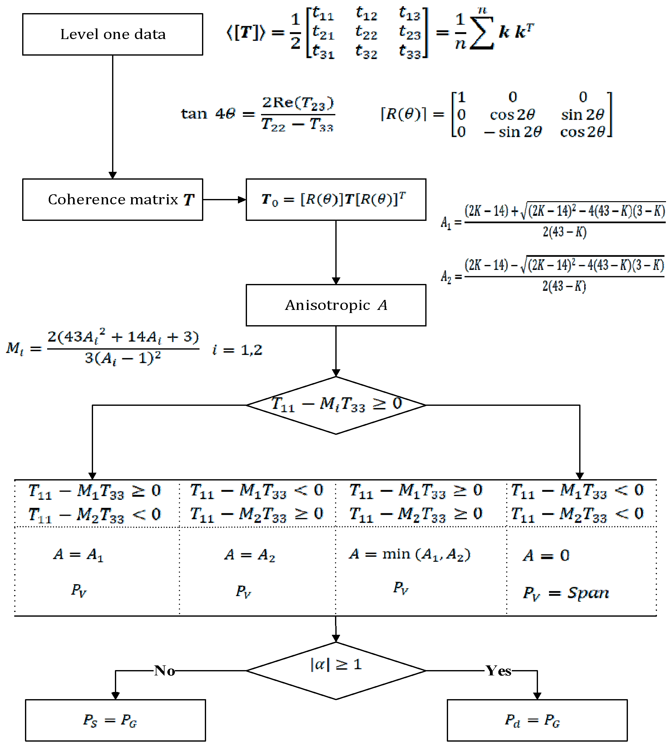
Therefore, the orientation angle compensation can somewhat solve the problem of overestimation of the volume scattering power component. At the same time, the increase in has obvious improvement regarding the problem of negative power value because one of the main reasons for the negative power value of surface scattering or double bounce scattering is that . For the second condition, we dealt with it using orientation angle compensation. So, the first condition will be our main basis for determining the adaptive parameters. Choosing a minimum A value that satisfies the first condition is the determined optimal parameter value. Figure 6 shows the whole process of this algorithm.
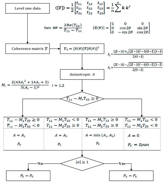
Figure 6.
The flowchart of the algorithm.
3. Results and Analysis
In order to verify the advantages of the algorithm proposed in this paper in the grassland polarimetric target decomposition algorithm, we implemented the algorithm in this paper on two experimental areas: the X-band COSMOS-SkyMed dataset of Xiwuqi grassland in the Inner Mongolia Autonomous Region and the C-band AirBorne dataset of Hunsandak grassland in the Inner Mongolia Autonomous Region. The third part of the paper will analyze the advantages of the algorithm from qualitative and quantitative perspectives, respectively, and to further illustrate the reliability of the algorithm, the experiment will also be compared with other algorithms on the premise of the same study areas.
3.1. Experiments on X-Band Data from the Grasslands of Xiwuqi in the Inner Mongolia Autonomous Region
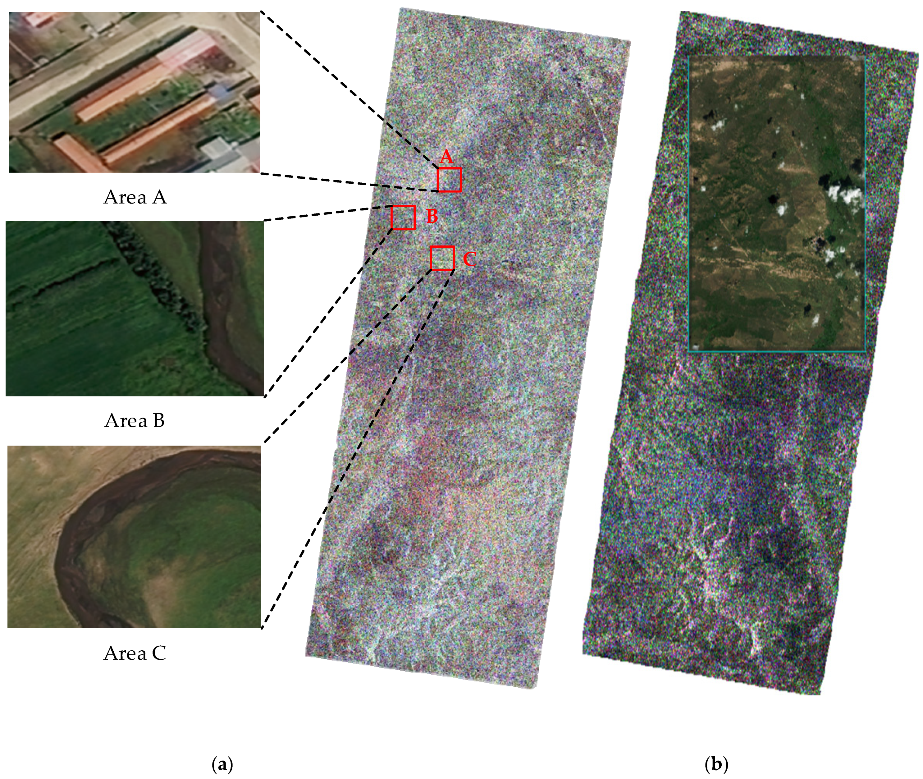
The spatial resolution of this dataset is 3m and the data collection date is 28 August 2023. The pixels of the original image were 17,953 × 7589. The corresponding PauliRGB image and optical image are shown in Figure 7. From the optical image, it can be seen that the grass in the test area is lush and covers a wide area.

Figure 7.
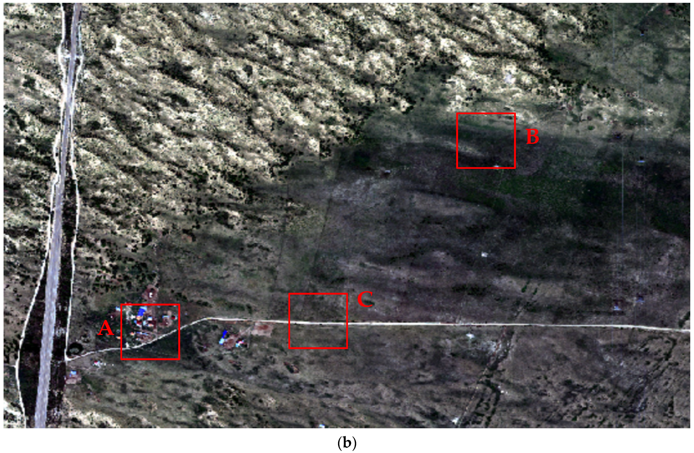
SAR image and optical image of the study area. (a) SAR image; A: located in urban area; B: located in grasslandarea; C: a relatively sparse area of grassland containing a road. (b) optical image of selected areas.
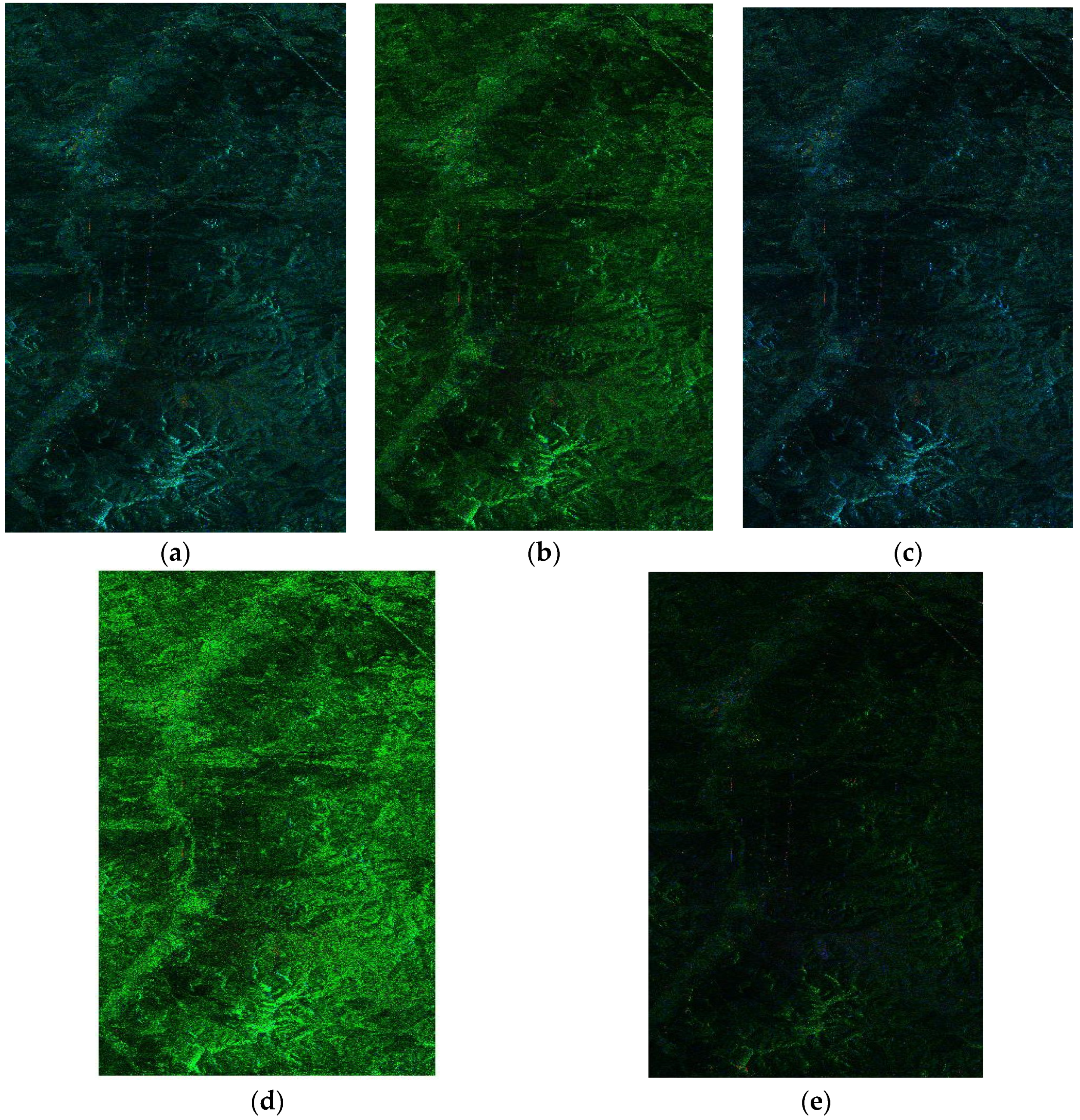
These five algorithms, FRE2 [49], Y4R [20], HTCD [51], OSM [52] and the algorithm of this paper, respectively, are used in an experiment on the experimental dataset, and the experimental results are shown by Figure 8. In order to have a more intuitive feel of the results of the experiments, the intensity of the scattering component at each pixel point is represented by the color in the pseudo-color composite map. The double bounce scattering power (Pd) is indicated by a red color, the volume scattering power (Pv) by a green color, and the surface scattering power (Pd) by a blue color. As a whole, the two algorithms, FRE2 and HTCD, show a blue-green color as a whole, and their volume scattering and surface scattering account for the main components, which is not in line with the characteristics of the grassland region. The Y4R and OSM algorithms show a green color as a whole, which indicates that the volume scattering accounts for the main components. However, it is not difficult to see that these two algorithms are fuzzy for the discrimination of bridges and roads in the figure, so the algorithm may have the problem of overestimation of volume scattering, and this speculation will be specifically verified in the subsequent quantitative analysis.
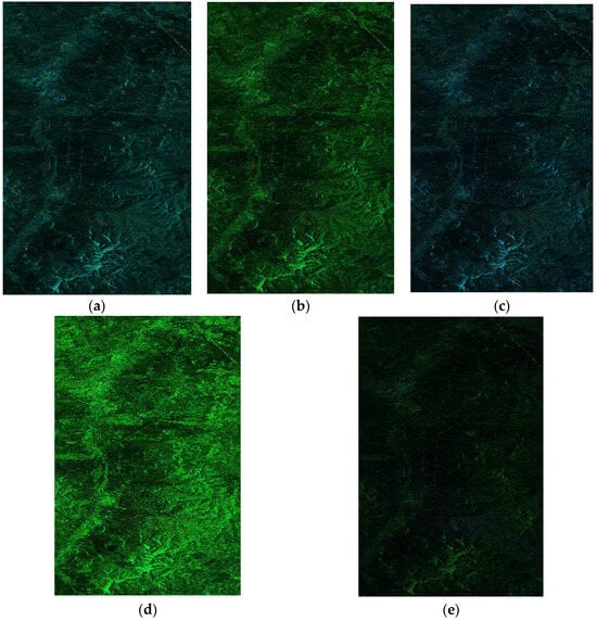
Figure 8.
RGB syntheses of polarimetric target decomposition algorithm. (a) FRE2; (b) Y4R; (c) HTCD; (d) OSM; (e) proposed.
The algorithm proposed in this paper with its overall green color, consistent with the characteristics of the grassland region, followed by the road and bridge in the figure can be seen in the approximate outline. In a comprehensive comparison, the algorithm proposed in this paper is more advantageous in the polarimeric decomposition of the grassland. The next quantitative analysis will further illustrate the advantages and disadvantages of each algorithm.
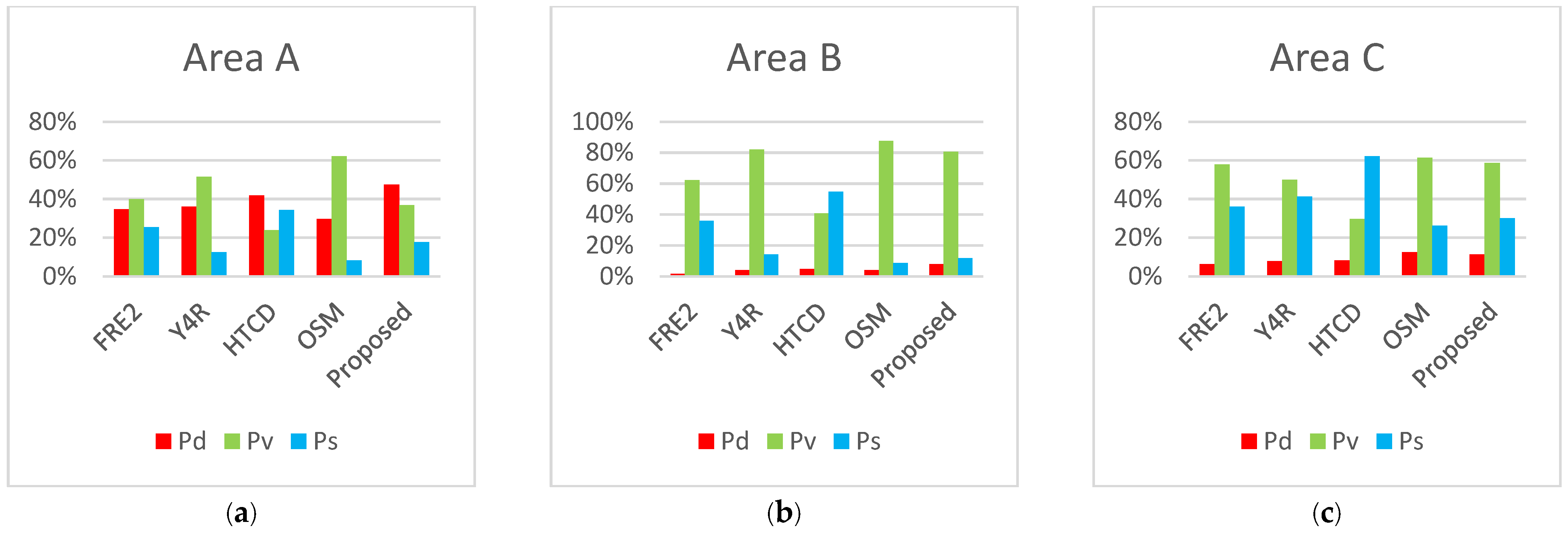
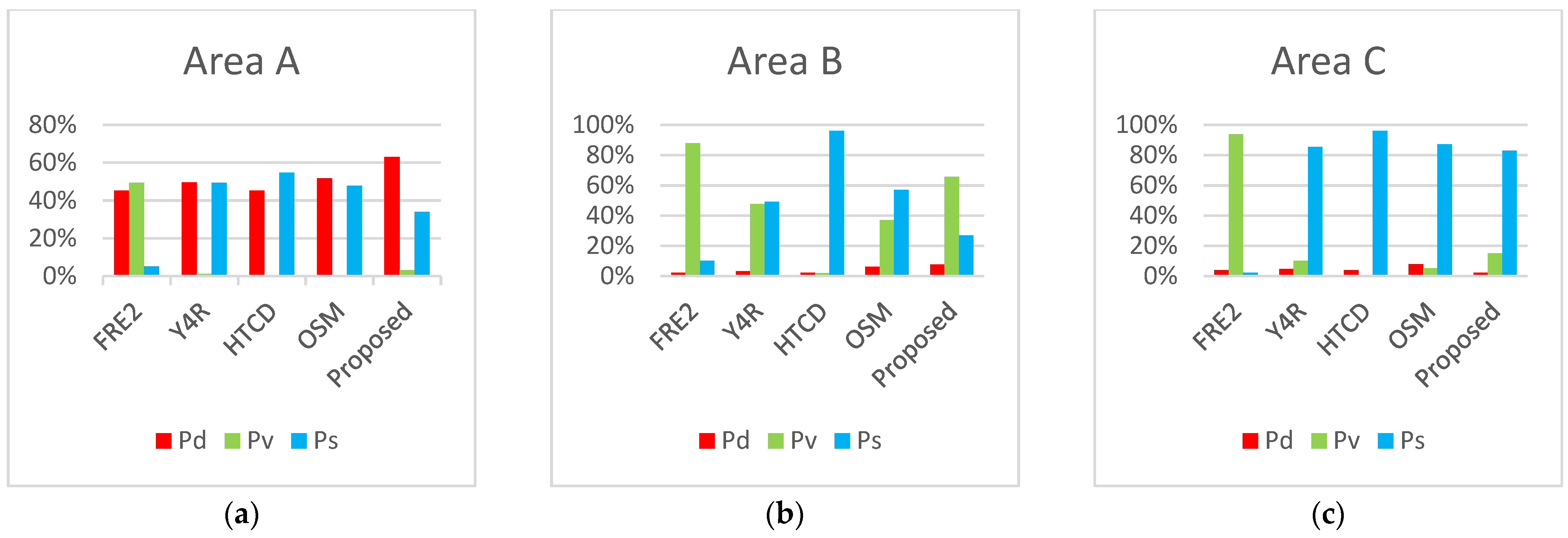
In order to quantitatively evaluate the scattering components, three well-characterized test areas were selected for the experiment for specific data analysis, as shown in Figure 7: Area A, located in the area of man-made buildings; area B, located in the area of municipal grassland; and area C, a relatively sparse area of grassland containing a highway. Table 1 gives the proportion of distribution of each polarimetric component in all methods for the three regions. In order to make the comparison between algorithms more obvious, we visualized Table 1 and generated a data bar graph, as shown in Figure 9. Figure 9 gives the percentage of polarimetric target decomposition components for each algorithm in regions A, B and C.

Table 1.
Percentage of each scattering component of grassland data in Xiwuqi, Inner Mongolia Autonomous Region, China (%).

Figure 9.
Histogram of the percentage of each scattering component of grassland data in Xiwuqi, Inner Mongolia Autonomous Region, China. (a) Area A; (b) area B; (c) area C.
For area A, which was chosen as it contained houses, roads and a small amount of vegetation, the scattering characteristics should be dominated by double bounce scattering, containing a certain proportion of volume scattering components and less surface scattering. Based on this judgment, the decomposition results of FRE2, Y4R and OSM are not consistent with the actual situation, and the decomposition results of all three algorithms are that the volume scattering has the highest proportion among the three components. Among them, the difference between double bounce scattering and volume scattering of Y4R is too large, and it is very likely that there is a decomposition problem with too high volume scattering. The decomposition results of the remaining two algorithms, on the other hand, are more in line with the actual situation. And the percentage difference between the algorithms and proposed in this paper is not much, which is more in line with the actual situation.
For area B, a region with lush grassland cover was chosen, and its scattering characteristics should be dominated by volume scattering, containing less surface scattering and double bounce scattering. Based on this judgment, the decomposition results of HTCD are not consistent with the actual situation, and the decomposition results of the algorithms are all that surface scattering has the highest proportion among the three components. The remaining four algorithms all conform to the actual situation, but the FRE2 algorithm has lower volume scattering; based on the actual optical image, it can be seen that the area is basically a region with more lush grass, and its volume scattering should be higher, and compared to the other algorithms, the volume scattering component of FRE2 is lower, which does not fit the actual situation closely.
For area C, a grassland area with relatively low grass cover and a river passing through the area is chosen, and its scattering characteristics should be dominated by volume scattering, but it is lower than that of region B, with a certain amount of surface scattering and double bounce scattering components. HTCD has too much double bounce scattering, which dominates the decomposition of the region, and the decomposition results are not in line with the actual situation. Although the remaining four cases are all consistent with the actual situation, the volume scattering and double bounce scattering share of FRE2 and Y4R are not very different, which are also inconsistent in the optical image; the decomposition results of these two algorithms are poorly fitted to the actual situation compared with the remaining two algorithms. In summary, the algorithm proposed in this paper has better decomposition results for the grassland region.
3.2. Experiments on C-Band Data from the Hunsandak Grassland in Inner Mongolia Autonomous Region
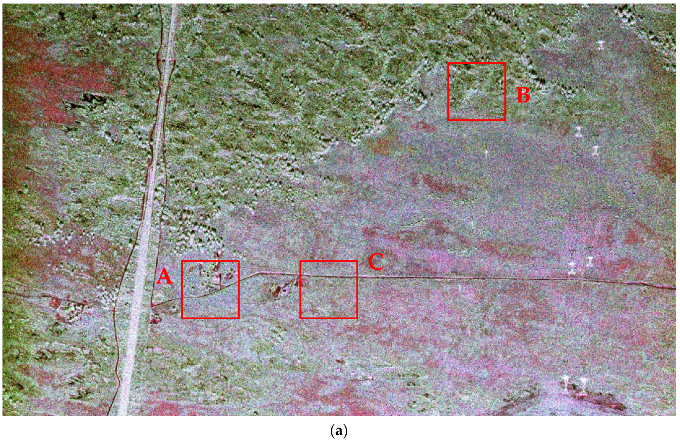
To further illustrate the effectiveness of the algorithm, a second experiment is conducted in this paper. The second experiment uses the C-band AirBorne dataset from the Hunshandak grassland region of Inner Mongolia with a spatial resolution of 1 m. The data were collected on 14 July 2021. The dataset contains the pixel number of 3027 × 4096. The corresponding PauliRGB image and optical image are shown in Figure 10. Based on the optical image of the experimental data area, it can be seen that the grass cover area in test area II is less compared to that in test area I. A certain area of bare ground exists.


Figure 10.
Pauli map and optical map of the study area. (a) Paili map; (b) optical map. A: located in urban area; B: located in grassland area; C: located in bare ground containing a road.
These five algorithms are used in an experiment on the experimental dataset, and the experimental results are shown by Figure 11. As a whole, the HTCD and OSM algorithms show a blue color as a whole, indicating that surface scattering is the main component. This is not consistent with the characteristics of the grassland region. This algorithm, FRE2, presents a green color as a whole, which is consistent with the characteristics of the grassland, but does not reflect the bare ground component, so the algorithm may have the problem of overestimation of volume scattering, and this speculation will be specifically verified in the subsequent quantitative analysis. The decomposition results of Y4R are roughly in line with the actual situation, but still, the surface scattering component is over-represented. Compared with the algorithm proposed in this paper, the algorithm proposed in this paper is in better agreement with the actual situation.
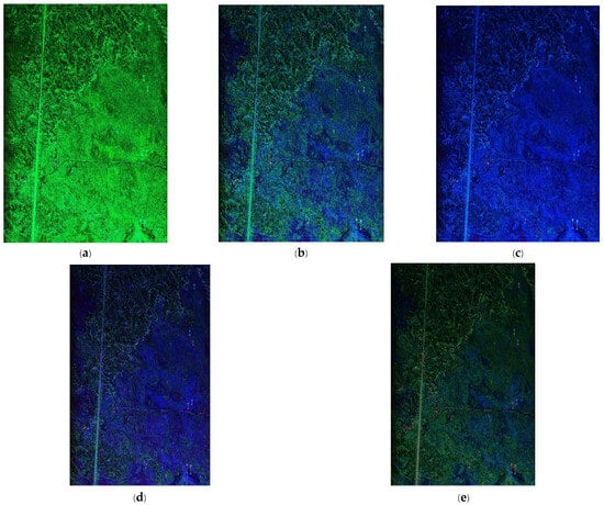
Figure 11.
Decomposition results of five algorithms in the Hunsandak grasslands. (a) FRE2; (b) Y4R; (c) HTCD; (d) OSM; (e) proposed.
In order to quantitatively evaluate the scattering components, we chose the following three well-characterized test areas for specific data analysis, as shown in Figure 10: area A, located in the area of man-made buildings; area B, in the area of grassland; and area C in the area of bare ground containing a road. Table 2 gives the proportion of the distribution of each polarimetric component in all methods for the three regions. To make the comparison between the algorithms more obvious, we visualized Table 2 and generated a data bar graph, as shown in Figure 12. Figure 12 gives the percentage of polarization target decomposition components for each algorithm in regions A, B and C.
Table 2.
Percentage of each scattering component of the Hunsandak Grassland data, Inner Mongolia Autonomous Region, China (%).
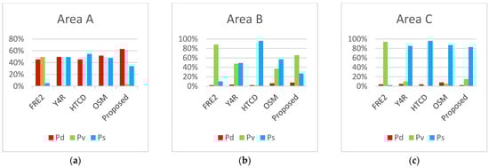
Figure 12.
Histogram of the percentage of each scattering component of the Hunsandak grassland data in the Inner Mongolia Autonomous Region. (a) Area A; (b) area B; (c) area C.
For area A, an area containing a house road and a certain area of bare ground was selected, and its scattering characteristics should be dominated by double bounce scattering, containing a certain proportion of surface scattering components and less volume scattering. Based on this judgment, the decomposition results of FRE2, Y4R and HTCD are not consistent with the actual situation. The volume scattering of FRE2 is the dominant component, while the surface scattering of HTCD is the dominant component, and the surface scattering and double bounce scattering of Y4R are almost the same, so the decomposition results of these three algorithms are not consistent with the actual situation. The decomposition results of OSM are consistent with the actual situation, but the advantages of double bounce scattering are not. The decomposition results of OSM are consistent with the actual situation, but the advantage of double bounce scattering is not obvious. The algorithm proposed in this paper has obvious advantages in double bounce scattering, which is more in line with the actual situation.
For area B, an area with lush grassland cover was selected for the study, and its scattering characteristics should be dominated by volume scattering, containing less surface scattering and double bounce scattering. Based on this judgment, the decomposition results of HTCD, Y4R and OSM are not consistent with the actual situation, and the algorithms’ decompositions all result in the highest proportion of surface scattering among the three components. The remaining two algorithms, both of which are realistic, have higher volume scattering for the FRE2 algorithm. Analyzing this in conjunction with Figure 11 shows that the FRE2 algorithm suffers from an overestimation of volume scattering.
For area C, a bare ground region with relatively low coverage and a highway passing through the region was chosen, and its scattering characteristics should be dominated by surface scattering, containing less surface scattering and double bounce scattering. The volume scattering of FRE2 is overestinated and dominates the decomposition of the region, which makes the decomposition results inconsistent with the actual situation. Although the remaining four cases are all consistent with the actual situation, the volume scattering of HTCD is zero, which is also seen to be inconsistent in the optical image. In summary, the algorithm proposed in this paper gives better decomposition results for the grassland region.
4. Conclusions
In this paper, an adaptive grassland scattering model decomposition with two-component decomposition as the basic framework is proposed. The model abstracts grass as a rotatable ellipsoid of variable shape from the perspective of polarization tensor and combines it with the actual grassland. Considering the presence of fallen grass in the real situation, the rotation is simulated in two dimensions: the tilt angle and canting angle. The degree of anisotropy A is directly introduced as a parameter to describe the shape of the grass. Finally, a novel volume scattering model is proposed by integration calculation. In the decomposition process, two-component decomposition is used as the basic framework, and the negative power minimization principle is used to determine the value of the parameter A to obtain the final decomposition result. In this paper, the validity of the method is verified using data from Xiwuqi and Hunshandak in Inner Mongolia. The experimental results show that the proposed method can obtain reasonable scattering mechanisms for various terrain types compared with algorithms such as FRE2, Y4R, HTCD, and OSM, and it is a more suitable decomposition algorithm for grasslands. During the experimental process, we found that the model proposed in this paper has some advantages in terms of vegetation coverage and road segmentation, which can be followed up in these two aspects.
Author Contributions
Conceptualization, P.H. and Y.C. (Yalan Chen); methodology, P.H. and Y.C. (Yalan Chen); software, P.H. and Y.C. (Yalan Chen); investigation, X.L. (Xiujuan Li) and W.T.; visualization, P.H., X.L. (Xiujuan Li) and B.L.; writing—original draft preparation, P.H., X.Y., Y.C. (Yuejuan Chen) and Y.D.; writing—review and editing, X.L. (Xiaoqi Lv), W.T. and Y.C. (Yalan Chen); project administration, P.H., X.L. (Xiujuan Li) and Y.D. All authors have read and agreed to the published version of the manuscript.
Funding
This research was funded in part by the Joint Funds of the National Natural Science Foundation of China (Grant No. U22A2010); in part by the National Natural Science Foundation of China (52064039 and 52304173); in part by the Center for Applied Mathematics of Inner Mongolia (Grant No. ZZYJZD2022001); in part by the Inner Mongolia Natural Science Foundation Program (Grant Nos. 2024MS06030 and 2024MS06004) and in part by the Basic Research Operating Expenses Program for Colleges and Universities directly under the Inner Mongolia Autonomous Region (Grant No. JY20220072).
Data Availability Statement
The data presented in this study are available upon request from the corresponding author. The data are not publicly available due to privacy.
Conflicts of Interest
The authors declare no conflicts of interest.
References
- Wang, B.; Tian, Z.; Zhang, W.; Chen, G.; Guo, Y.; Wang, M. Retrieval of Green-up Onset Date From MODIS Derived NDVI in Grasslands of Inner Mongolia. IEEE Access 2019, 7, 77885–77893. [Google Scholar] [CrossRef]
- Stiles, J.M.; Sarabandi, K. Electromagnetic scattering from grassland. I. A fully phase-coherent scattering model. IEEE Trans. Geosci. Remote Sens. 2000, 38, 339–348. [Google Scholar] [CrossRef]
- Ali, I.; Cawkwell, F.; Dwyer, E.; Barrett, B.; Green, S. Satellite remote sensing of grasslands: From observation to management. J. Plant Ecol. 2016, 9, 649–671. [Google Scholar] [CrossRef]
- Chen, S.-W.; Xuesong, W.; Xiao, S.-P.; Sato, M. Target Scattering Mechanism in Polarimetric Synthetic Aperture Radar—Interpretation and Application; Springer: Singapore, 2018. [Google Scholar]
- Jawak, S. A Review on Applications of Imaging Synthetic Aperture Radar with a Special Focus on Cryospheric Studies. Adv. Remote Sens. 2015, 4, 163–175. [Google Scholar] [CrossRef]
- Wang, X.; Zhang, L.; Zou, B. A new Six-Component Decomposition based on New Volume Scattering Models for PolSAR Image. In Proceedings of the 2021 CIE International Conference on Radar (Radar), Haikou, China, 15–19 December 2021; pp. 631–634. [Google Scholar]
- Huynen, J.R. Phenomenological Theory of Radar Targets. Ph.D. Thesis, Electrical Engineering, Mathematics and Computer Science (EEMCS) (TU Delft), Delft, The Netherlands, 1970. [Google Scholar]
- Cloude, S.R.; Pottier, E. A review of target decomposition theorems in radar polarimetry. IEEE Trans. Geosci. Remote Sens. 1996, 34, 498–518. [Google Scholar] [CrossRef]
- Holm, W.A.; Barnes, R.M. On radar polarization mixed target state decomposition techniques. In Proceedings of the 1988 IEEE National Radar Conference, Ann Arbor, MI, USA, 20–21 April 1988; pp. 249–254. [Google Scholar]
- Cloude, S.R.; Pottier, E. An entropy based classification scheme for land applications of polarimetric SAR. IEEE Trans. Geosci. Remote Sens. 1997, 35, 68–78. [Google Scholar] [CrossRef]
- An, W.; Cui, Y.; Yang, J.; Zhang, H. Fast Alternatives to $H/\alpha$ for Polarimetric SAR. IEEE Geosci. Remote Sens. Lett. 2010, 7, 343–347. [Google Scholar] [CrossRef]
- Freeman, A.; Durden, S.L. A three-component scattering model for polarimetric SAR data. IEEE Trans. Geosci. Remote Sens. 1998, 36, 963–973. [Google Scholar] [CrossRef]
- Moriyama, T.; Uratsuka, S.; Umehara, T.; Maeno, H.; Satake, M.; Nadai, A.; Nakamura, K.J.I.T.C. Polarimetric SAR Image Analysis Using Model Fit for Urban Structures. IEICE Trans. Commun. 2005, 88-B, 1234–1243. [Google Scholar]
- Yamaguchi, Y.; Moriyama, T.; Ishido, M.; Yamada, H. Four-component scattering model for polarimetric SAR image decomposition. IEEE Trans. Geosci. Remote Sens. 2005, 43, 1699–1706. [Google Scholar] [CrossRef]
- Dou, Q.; Xie, Q.; Peng, X.; Lai, K.; Wang, J.; Lopez-Sanchez, J.M.; Shang, J.; Shi, H.; Fu, H.; Zhu, J. Soil moisture retrieval over crop fields based on two-component polarimetric decomposition: A comparison of generalized volume scattering models. J. Hydrol. 2022, 615, 128696. [Google Scholar] [CrossRef]
- Yin, J.; Yang, J. Target Decomposition Based on Symmetric Scattering Model for Hybrid Polarization SAR Imagery. IEEE Geosci. Remote Sens. Lett. 2021, 18, 494–498. [Google Scholar] [CrossRef]
- Yajima, Y.; Yamaguchi, Y.; Sato, R.; Yamada, H.; Boerner, W.M. POLSAR Image Analysis of Wetlands Using a Modified Four-Component Scattering Power Decomposition. IEEE Trans. Geosci. Remote Sens. 2008, 46, 1667–1673. [Google Scholar] [CrossRef]
- Singh, G.; Yamaguchi, Y. Model-Based Six-Component Scattering Matrix Power Decomposition. IEEE Trans. Geosci. Remote Sens. 2018, 56, 5687–5704. [Google Scholar] [CrossRef]
- Singh, G.; Malik, R.; Mohanty, S.; Rathore, V.S.; Yamada, K.; Umemura, M.; Yamaguchi, Y. Seven-Component Scattering Power Decomposition of POLSAR Coherency Matrix. IEEE Trans. Geosci. Remote Sens. 2019, 57, 8371–8382. [Google Scholar] [CrossRef]
- Yamaguchi, Y.; Sato, A.; Boerner, W.M.; Sato, R.; Yamada, H. Four-Component Scattering Power Decomposition With Rotation of Coherency Matrix. IEEE Trans. Geosci. Remote Sens. 2011, 49, 2251–2258. [Google Scholar] [CrossRef]
- An, W.; Cui, Y.; Yang, J. Three-Component Model-Based Decomposition for Polarimetric SAR Data. IEEE Trans. Geosci. Remote Sens. 2010, 48, 2732–2739. [Google Scholar] [CrossRef]
- Lee, J.S.; Ainsworth, T.L. The Effect of Orientation Angle Compensation on Coherency Matrix and Polarimetric Target Decompositions. IEEE Trans. Geosci. Remote Sens. 2011, 49, 53–64. [Google Scholar] [CrossRef]
- Yamaguchi, Y.; Singh, G.; Park, S.E.; Yamada, H. Scattering power decomoosition using fully polarimetric information. In Proceedings of the 2012 IEEE International Geoscience and Remote Sensing Symposium, Munich, Germany, 22–27 July 2012; pp. 91–94. [Google Scholar]
- Li, H.; Li, Q.; Wu, G.; Chen, J.; Liang, S. Adaptive Two-Component Model-Based Decomposition for Polarimetric SAR Data Without Assumption of Reflection Symmetry. IEEE Trans. Geosci. Remote Sens. 2017, 55, 197–211. [Google Scholar] [CrossRef]
- An, W.; Lin, M. A Reflection Symmetry Approximation of Multilook Polarimetric SAR Data and its Application to Freeman–Durden Decomposition. IEEE Trans. Geosci. Remote Sens. 2019, 57, 3649–3660. [Google Scholar] [CrossRef]
- Zyl, J.J.V.; Arii, M.; Kim, Y. Model-Based Decomposition of Polarimetric SAR Covariance Matrices Constrained for Nonnegative Eigenvalues. IEEE Trans. Geosci. Remote Sens. 2011, 49, 3452–3459. [Google Scholar] [CrossRef]
- Cloude, S. Polarisation: Applications in Remote Sensing; Oxford Academic: Oxford, UK, 2009. [Google Scholar] [CrossRef]
- Cui, Y.; Yamaguchi, Y.; Yang, J.; Kobayashi, H.; Park, S.E.; Singh, G. On Complete Model-Based Decomposition of Polarimetric SAR Coherency Matrix Data. IEEE Trans. Geosci. Remote Sens. 2014, 52, 1991–2001. [Google Scholar] [CrossRef]
- Zou, B.; Lu, D.; Zhang, L.; Moon, W.M. Eigen-Decomposition-Based Four-Component Decomposition for PolSAR Data. IEEE J. Sel. Top. Appl. Earth Obs. Remote Sens. 2016, 9, 1286–1296. [Google Scholar] [CrossRef]
- Maurya, H.; Bhattacharya, A.; Mishra, A.K.; Panigrahi, R.K. Hybrid Three-Component Scattering Power Characterization From Polarimetric SAR Data Isolating Dominant Scattering Mechanisms. IEEE Trans. Geosci. Remote Sens. 2022, 60, 4415315. [Google Scholar] [CrossRef]
- Neumann, M.; Ferro-Famil, L.; Reigber, A. Estimation of Forest Structure, Ground, and Canopy Layer Characteristics From Multibaseline Polarimetric Interferometric SAR Data. IEEE Trans. Geosci. Remote Sens. 2010, 48, 1086–1104. [Google Scholar] [CrossRef]
- Arii, M.; Zyl, J.J.V.; Kim, Y. A General Characterization for Polarimetric Scattering From Vegetation Canopies. IEEE Trans. Geosci. Remote Sens. 2010, 48, 3349–3357. [Google Scholar] [CrossRef]
- Lee, J.-S.; Ainsworth, T.L.; Wang, Y. Generalized Polarimetric Model-Based Decompositions Using Incoherent Scattering Models. IEEE Trans. Geosci. Remote Sens. 2014, 52, 2474–2491. [Google Scholar] [CrossRef]
- Chen, S.W.; Wang, X.S.; Xiao, S.P.; Sato, M. General Polarimetric Model-Based Decomposition for Coherency Matrix. IEEE Trans. Geosci. Remote Sens. 2014, 52, 1843–1855. [Google Scholar] [CrossRef]
- Arii, M.; van Zyl, J.J.; Kim, Y. Adaptive Model-Based Decomposition of Polarimetric SAR Covariance Matrices. IEEE Trans. Geosci. Remote Sens. 2011, 49, 1104–1113. [Google Scholar] [CrossRef]
- Antropov, O.; Rauste, Y.; Hame, T. Volume Scattering Modeling in PolSAR Decompositions: Study of ALOS PALSAR Data Over Boreal Forest. IEEE Trans. Geosci. Remote Sens. 2011, 49, 3838–3848. [Google Scholar] [CrossRef]
- Huang, X.; Wang, J.; Shang, J. An Adaptive Two-Component Model-Based Decomposition on Soil Moisture Estimation for C-Band RADARSAT-2 Imagery Over Wheat Fields at Early Growing Stages. IEEE Geosci. Remote Sens. Lett. 2016, 13, 414–418. [Google Scholar] [CrossRef]
- Wang, Z.; Zeng, Q.; Jiao, J. An adaptive decomposition approach with dipole aggregation model for polarimetric sar data. Remote Sens. 2021, 13, 2583. [Google Scholar] [CrossRef]
- Wang, T.; Suo, Z.; Jiang, P.; Ti, J.; Ding, Z.; Qin, T. An Optimal Polarization SAR Three-Component Target Decomposition Based on Semi-Definite Programming. Remote Sens. 2023, 15, 5292. [Google Scholar] [CrossRef]
- Chen, S.W.; Sato, M. Tsunami Damage Investigation of Built-Up Areas Using Multitemporal Spaceborne Full Polarimetric SAR Images. IEEE Trans. Geosci. Remote Sens. 2013, 51, 1985–1997. [Google Scholar] [CrossRef]
- Zhang, L.; Zou, B.; Cai, H.; Zhang, Y. Multiple-Component Scattering Model for Polarimetric SAR Image Decomposition. IEEE Geosci. Remote Sens. Lett. 2008, 5, 603–607. [Google Scholar] [CrossRef]
- Xiang, D.; Ban, Y.; Su, Y. Model-Based Decomposition With Cross Scattering for Polarimetric SAR Urban Areas. IEEE Geosci. Remote Sens. Lett. 2015, 12, 2496–2500. [Google Scholar] [CrossRef]
- Hajnsek, I.; Pottier, E.; Cloude, S.R. Inversion of surface parameters from polarimetric SAR. IEEE Trans. Geosci. Remote Sens. 2003, 41, 727–744. [Google Scholar] [CrossRef]
- Lee, J.-S.; Pottier, E. Polarimetric Radar Imaging: From Basics to Applications; Routledge: London, UK, 2009. [Google Scholar]
- Manuel, L.-S.J. Analysis and Estimation of Biophysical Parameters of Vegetation by Radar Polarimetry. Ph.D. Thesis, Universidad Politecnica de Valencia, Valencia, Spain, 2000. [Google Scholar]
- Karam, M.A.; Fung, A.K. Electromagnetic scattering from a layer of finite length, randomly oriented, dielectric, circular cylinders over a rough interface with application to vegetation. Int. J. Remote Sens. 1988, 9, 1109–1134. [Google Scholar] [CrossRef]
- Li, X.; Liu, Y.; Huang, P.; Liu, X.; Tan, W.; Fu, W.; Li, C. A Hybrid Polarimetric Target Decomposition Algorithm with Adaptive Volume Scattering Model. Remote Sens. 2022, 14, 2441. [Google Scholar] [CrossRef]
- Monsivais-Huertero, A.; Sarabandi, K.; Chenerie, I. Multipolarization Microwave Scattering Model for Sahelian Grassland. IEEE Trans. Geosci. Remote Sens. 2010, 48, 1416–1432. [Google Scholar] [CrossRef]
- Freeman, A. Fitting a Two-Component Scattering Model to Polarimetric SAR Data From Forests. IEEE Trans. Geosci. Remote Sens. 2007, 45, 2583–2592. [Google Scholar] [CrossRef]
- Chen, S.W.; Ohki, M.; Shimada, M.; Sato, M. Deorientation Effect Investigation for Model-Based Decomposition Over Oriented Built-Up Areas. IEEE Geosci. Remote Sens. Lett. 2013, 10, 273–277. [Google Scholar] [CrossRef]
- Maurya, H.; Panigrahi, R. Non-Negative Scattering Power Decomposition for PolSAR Data Interpretation. IET Radar Sonar Navig. 2018, 12, 593–602. [Google Scholar] [CrossRef]
- Han, W.; Fu, H.; Zhu, J.; Xie, Q.; Zhang, S. Orthogonal Scattering Model-Based Three-Component Decomposition of Polarimetric SAR Data. Remote Sens. 2022, 14, 4326. [Google Scholar] [CrossRef]


Disclaimer/Publisher’s Note: The statements, opinions and data contained in all publications are solely those of the individual author(s) and contributor(s) and not of MDPI and/or the editor(s). MDPI and/or the editor(s) disclaim responsibility for any injury to people or property resulting from any ideas, methods, instructions or products referred to in the content. |
© 2024 by the authors. Licensee MDPI, Basel, Switzerland. This article is an open access article distributed under the terms and conditions of the Creative Commons Attribution (CC BY) license (https://creativecommons.org/licenses/by/4.0/).