

Complex-Valued 2D-3D Hybrid Convolutional Neural Network with Attention Mechanism for PolSAR Image Classification


Abstract

1. Introduction
- An innovative hybrid CV-CNN for PolSAR image classification is presented, which effectively incorporates the advantages of both 2D and 3D convolution. Specifically, the model first extracts spatial features using complex-valued 2D convolutions with fewer parameters and then integrates spatial and channel dimensional features using 3D convolutions. Compared with a single-dimensional CNN, this hybrid network effectively reduces the number of parameters to avoid overfitting while maintaining better performance.
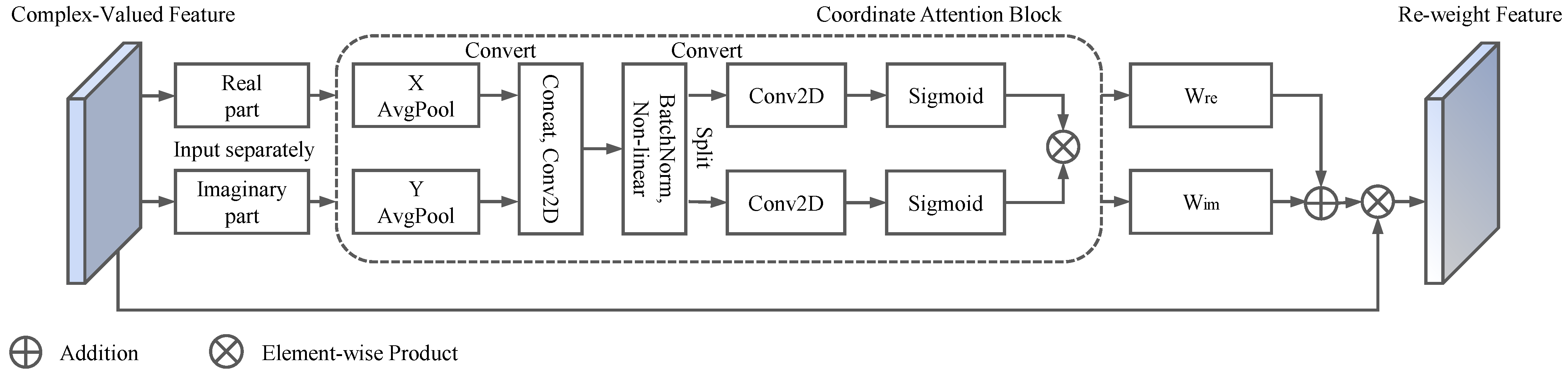
- We design an attention block for CV-CNN to increase the model’s efficiency and accuracy. The proposed attention block utilizes both the real and imaginary parts of features to calculate weights that represent feature importance. The classification results can effectively be improved through the utilization of recalibrated features supplemented with appropriate weights. It is worth noting that the inputs and outputs of the block are in complex form.
- Experiments are performed on three authentic PolSAR datasets to confirm the advancement of our proposed method. Under the same conditions, CV-2D/3D-CNN-AM provides a competitive classification outcome, which effectively extracts discriminative features and focuses on more significant information.
2. Related Work
2.1. PolSAR Data Processing
2.2. CV-CNN-Based PolSAR Classification Methods
2.3. Attention Mechanisms
3. Proposed Method
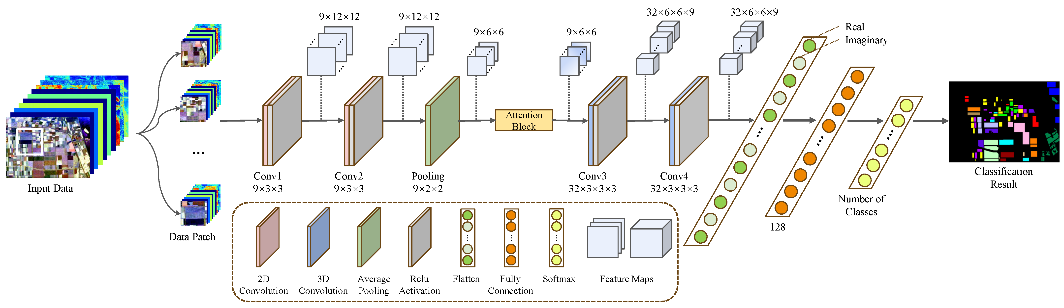
3.1. Framework of CV-2D/3D-CNN-AM
3.2. Complex-Valued 2D-3D Hybrid CNN
3.3. Improved Attention Block for Complex-Valued Tensors
4. Experiments
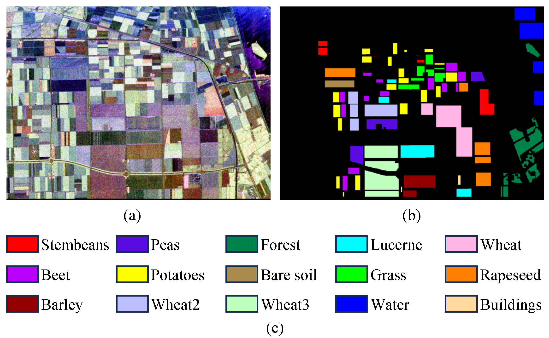
4.1. Datasets
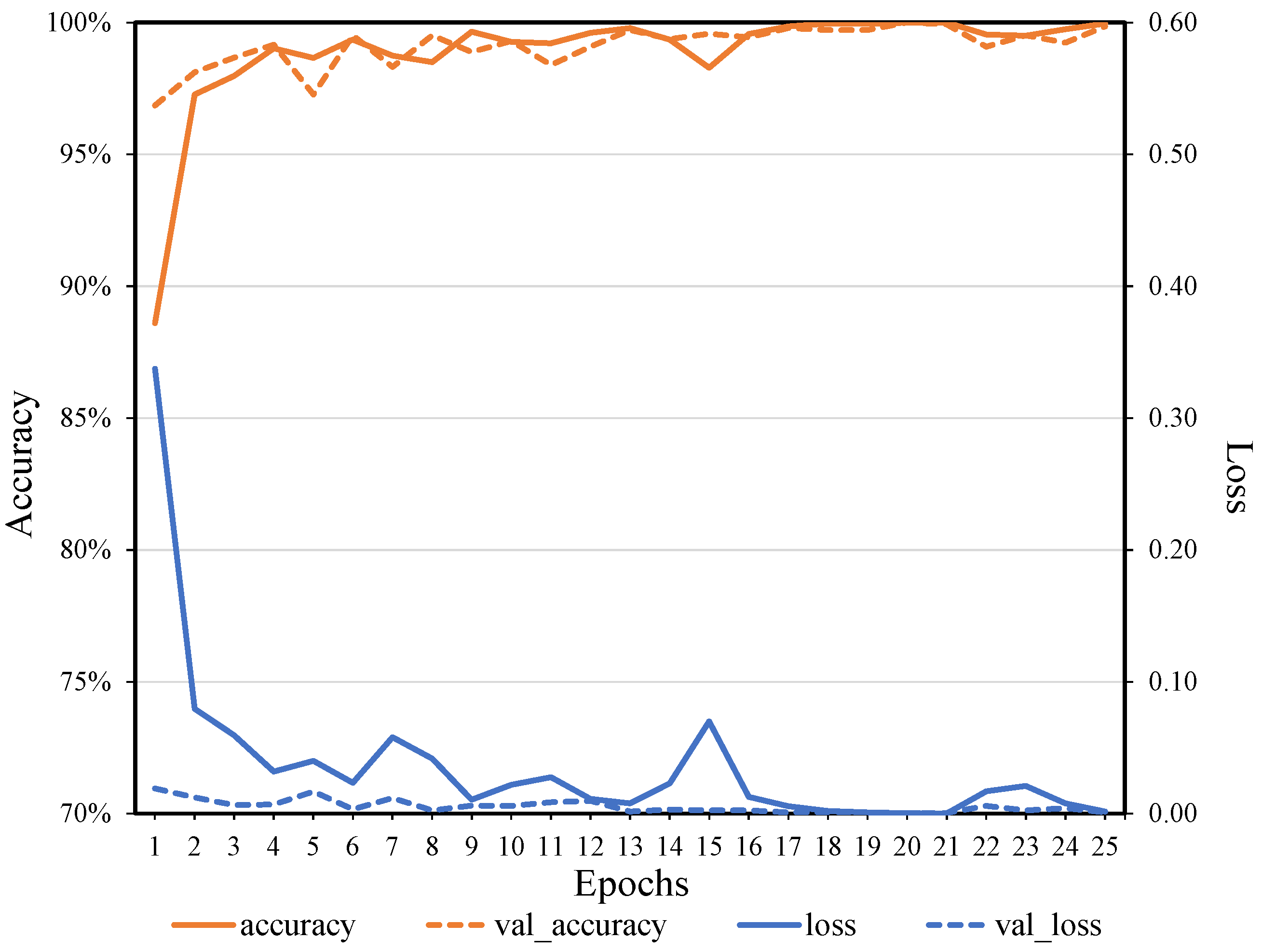
4.2. Experimental Setting
- SVM: SVM is a classical and powerful supervised machine learning technique. It finds an optimal hyperplane in pixel-level classification by maximizing the distance between pixels of different categories to determine the categories. Specifically, SVM is based on kernels that map the data into a high-dimensional space to make them linearly divisible, thus solving the non-linear problems well.
- CV-MLP: CV-MLP uses a stack of fully connected layers to map the input image data into high-dimensional features. It extracts and transforms the features through hidden layers to learn the non-linear relationship between data and labels.
- CV-2D-CNN/CV-3D-CNN: Both CV-2D-CNN and CV-3D-CNN are capable of hierarchically extracting local abstract features for pixel classification. They are major deep neural networks. However, CV-2D-CNN extracts features in spatial dimensions under channel independence, while CV-3D-CNN can simultaneously process information in three dimensions.
- CV-FCN: CV-FCN learns the mapping between each pixel and its label end-to-end during classification. It eliminates the computational redundancy arising from the need to input a fixed-size patch around the center pixel when identifying it. Moreover, CV-FCN uses inverse convolution to upsample the extracted features and adapts well to inputs of arbitrary size.
- CNN-WT: CNN-WT is a new method based on deep neural networks and wavelet transform. It notes that the amount of PolSAR data is not enough to support a network with many layers, and the data are noisy. CNN-WT uses the wavelet transform for feature extraction and denoising of the raw data and feeds them into a multi-branch deep network for classification.
- PolSF: PolSF is a recently proposed PolSAR classification method for extracting abstract features based on the transformer framework. It analyzes complex dependencies within a region through a special local attention mechanism. Compared with shallow CNN models, PolSF has deeper layers and stronger feature extraction capability.
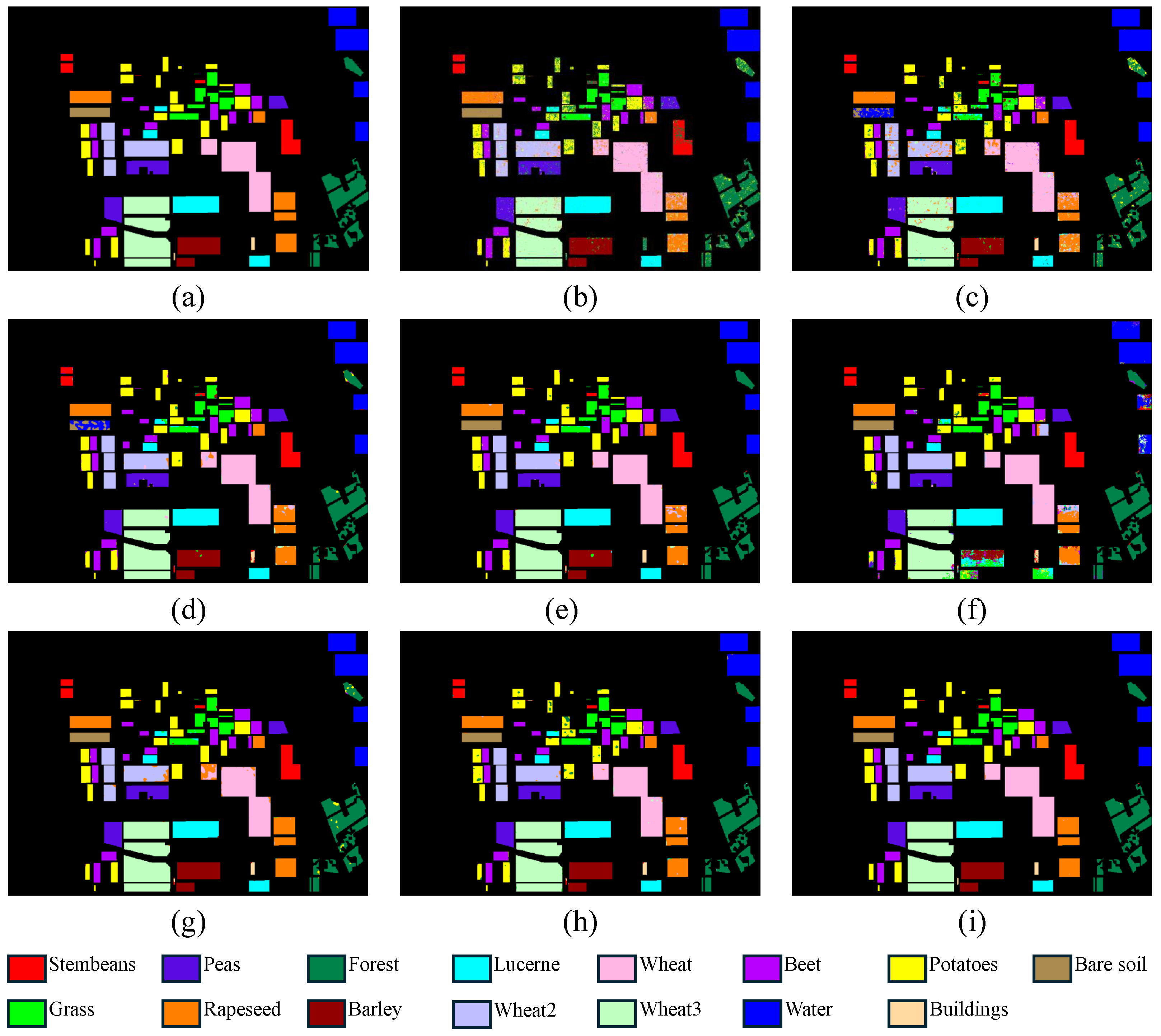
4.3. Experimental Results of Flevoland
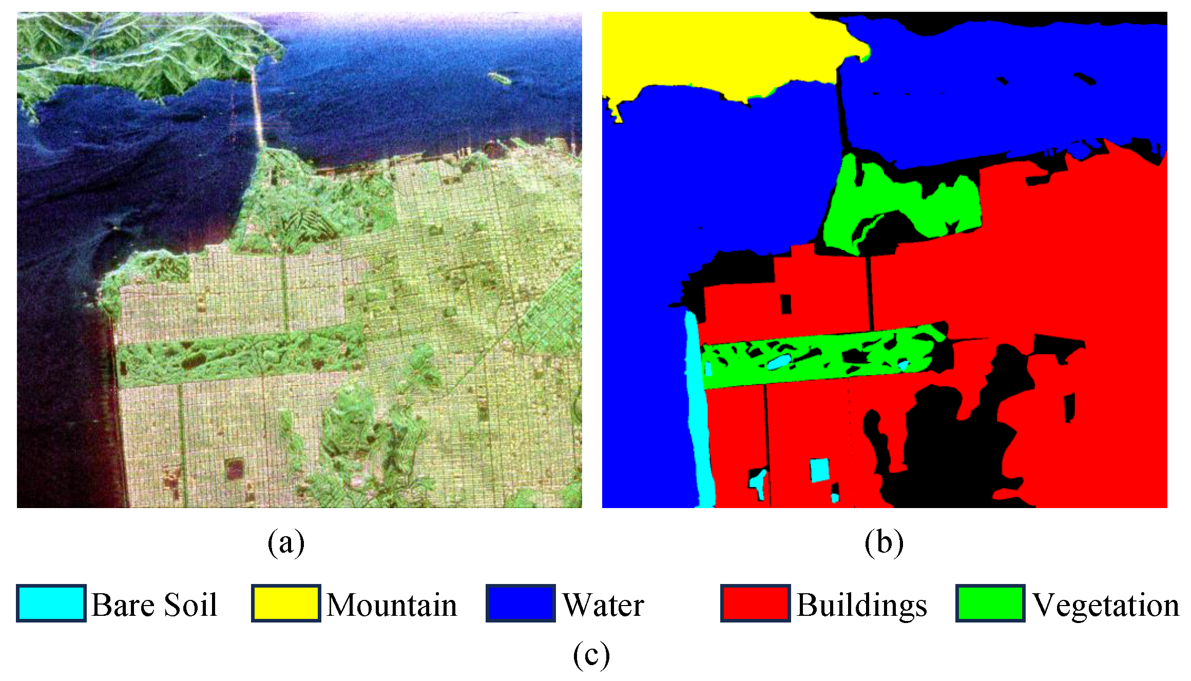
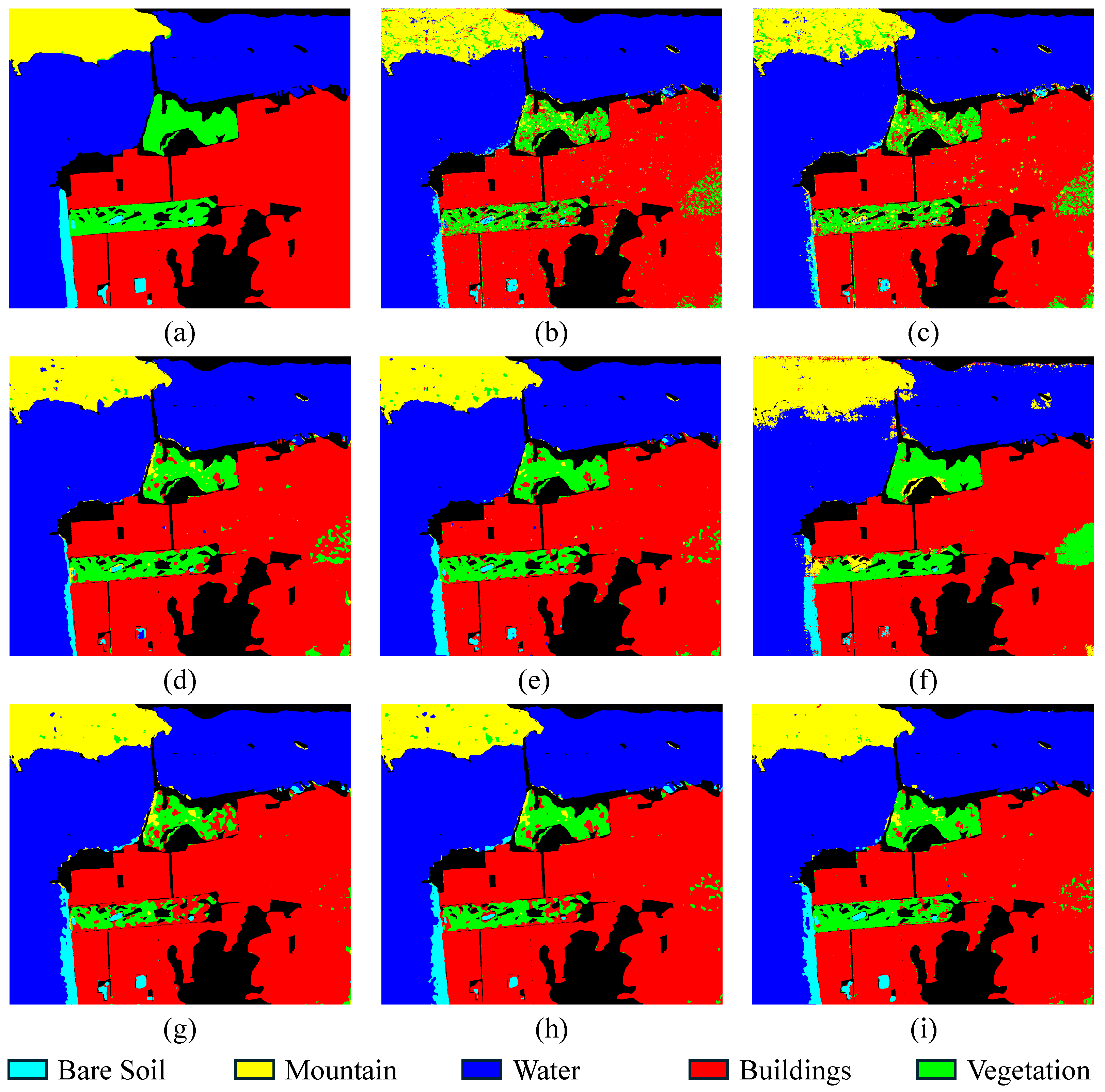
4.4. Experimental Results of San Francisco
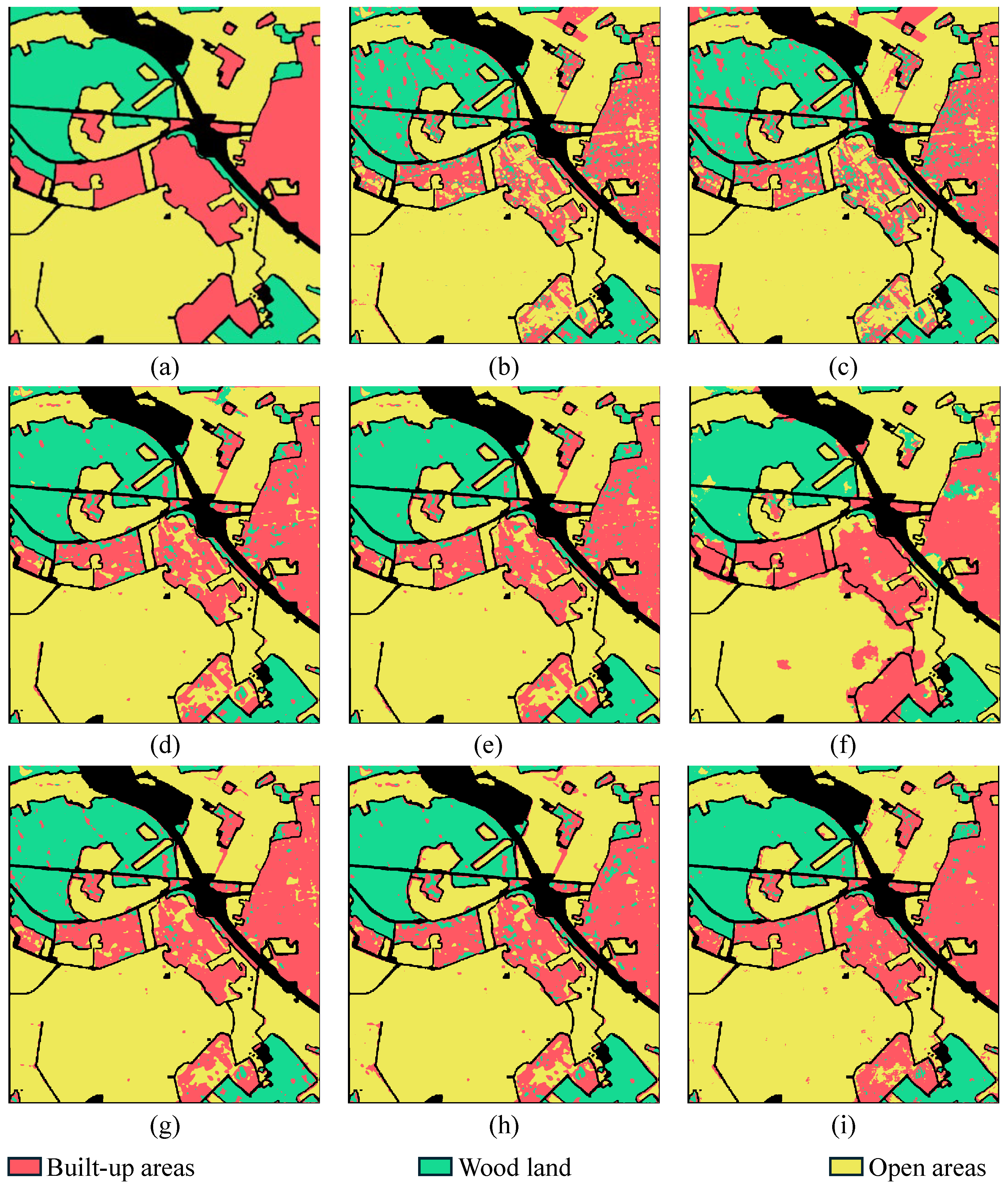
4.5. Experimental Results of Oberpfaffenhofen
4.6. Ablation Study
5. Conclusions
Author Contributions
Funding
Data Availability Statement
Conflicts of Interest
References
- Li, H.; Li, Q.; Wu, G.; Chen, J.; Liang, S. The Impacts of Building Orientation on Polarimetric Orientation Angle Estimation and Model-Based Decomposition for Multilook Polarimetric SAR Data in Urban Areas. IEEE Trans. Geosci. Remote Sens. 2016, 54, 5520–5532. [Google Scholar] [CrossRef]
- Yuzugullu, O.; Erten, E.; Hajnsek, I. Morphology estimation of rice fields using X-band PolSAR data. In Proceedings of the 2016 IEEE International Geoscience and Remote Sensing Symposium (IGARSS), Beijing, China, 10–15 July2016; pp. 7121–7124. [Google Scholar]
- Whitcomb, J.; Chen, R.; Clewley, D.; Kimball, J.; Pastick, N.; Yi, Y.; Moghaddam, M. Active Layer Thickness Throughout Northern Alaska by Upscaling from P-Band Polarimetric Sar Retrievals. In Proceedings of the IGARSS 2022—2022 IEEE International Geoscience and Remote Sensing Symposium, Kuala Lumpur, Malaysia, 17–22 July 2022; pp. 3660–3663. [Google Scholar] [CrossRef]
- Zhang, T.; Quan, S.; Wang, W.; Guo, W.; Zhang, Z.; Yu, W. Information Reconstruction-Based Polarimetric Covariance Matrix for PolSAR Ship Detection. IEEE Trans. Geosci. Remote Sens. 2023, 61, 5202815. [Google Scholar] [CrossRef]
- Ortiz, G.P.; Lorenzzetti, J.A. Observing Multimodal Ocean Wave Systems by a Multiscale Analysis of Polarimetric SAR Imagery. IEEE Geosci. Remote Sens. Lett. 2018, 15, 1735–1739. [Google Scholar] [CrossRef]
- Pottier, E. Dr. JR Huynen’s main contributions in the development of polarimetric radar techniques and how the ‘Radar Targets Phenomenological Concept’ becomes a theory. In Proceedings of the Radar Polarimetry, SPIE, San Diego, CA, USA, 22–22 July 1993; Volume 1748, pp. 72–85. [Google Scholar]
- Cloude, S.R.; Pottier, E. A review of target decomposition theorems in radar polarimetry. IEEE Trans. Geosci. Remote Sens. 1996, 34, 498–518. [Google Scholar] [CrossRef]
- Cloude, S.R.; Pottier, E. An entropy based classification scheme for land applications of polarimetric SAR. IEEE Trans. Geosci. Remote Sens. 1997, 35, 68–78. [Google Scholar] [CrossRef]
- Krogager, E.; Boerner, W.M.; Madsen, S.N. Feature-motivated Sinclair matrix (sphere/diplane/helix) decomposition and its application to target sorting for land feature classification. In Proceedings of the Wideband Interferometric Sensing and Imaging Polarimetry, SPIE, San Diego, CA, USA, 27 July–1 August 1997; Volume 3120, pp. 144–154. [Google Scholar]
- Cameron, W.L.; Leung, L.K. Feature motivated polarization scattering matrix decomposition. In Proceedings of the IEEE International Conference on Radar, Arlington, VA, USA, 7–10 May 1990; pp. 549–557. [Google Scholar]
- Freeman, A.; Durden, S.L. A three-component scattering model for polarimetric SAR data. IEEE Trans. Geosci. Remote Sens. 1998, 36, 963–973. [Google Scholar] [CrossRef]
- Lardeux, C.; Frison, P.L.; Tison, C.; Souyris, J.C.; Stoll, B.; Fruneau, B.; Rudant, J.P. Support vector machine for multifrequency SAR polarimetric data classification. IEEE Trans. Geosci. Remote Sens. 2009, 47, 4143–4152. [Google Scholar] [CrossRef]
- Liu, W.; Yang, J.; Li, P.; Han, Y.; Zhao, J.; Shi, H. A novel object-based supervised classification method with active learning and random forest for PolSAR imagery. Remote Sens. 2018, 10, 1092. [Google Scholar] [CrossRef]
- Yin, Q.; Cheng, J.; Zhang, F.; Zhou, Y.; Shao, L.; Hong, W. Interpretable POLSAR image classification based on adaptive-dimension feature space decision tree. IEEE Access 2020, 8, 173826–173837. [Google Scholar] [CrossRef]
- Zhang, S.; Cui, L.; Zhang, Y.; Xia, T.; Dong, Z.; An, W. Research on Input Schemes for Polarimetric SAR Classification Using Deep Learning. Remote Sens. 2024, 16, 1826. [Google Scholar] [CrossRef]
- Li, Z.; Huang, H.; Zhang, Z.; Shi, G. Manifold-based multi-deep belief network for feature extraction of hyperspectral image. Remote Sens. 2022, 14, 1484. [Google Scholar] [CrossRef]
- Zhang, W.T.; Wang, M.; Guo, J.; Lou, S.T. Crop classification using MSCDN classifier and sparse auto-encoders with non-negativity constraints for multi-temporal, Quad-Pol SAR data. Remote Sens. 2021, 13, 2749. [Google Scholar] [CrossRef]
- Seydi, S.T.; Hasanlou, M.; Amani, M. A new end-to-end multi-dimensional CNN framework for land cover/land use change detection in multi-source remote sensing datasets. Remote Sens. 2020, 12, 2010. [Google Scholar] [CrossRef]
- Hochstuhl, S.; Pfeffer, N.; Thiele, A.; Hammer, H.; Hinz, S. Your Input Matters—Comparing Real-Valued PolSAR Data Representations for CNN-Based Segmentation. Remote Sens. 2023, 15, 5738. [Google Scholar] [CrossRef]
- Zhou, Y.; Wang, H.; Xu, F.; Jin, Y.Q. Polarimetric SAR image classification using deep convolutional neural networks. IEEE Geosci. Remote Sens. Lett. 2016, 13, 1935–1939. [Google Scholar] [CrossRef]
- Zhang, L.; Chen, Z.; Zou, B.; Gao, Y. Polarimetric SAR terrain classification using 3D convolutional neural network. In Proceedings of the IGARSS 2018-2018 IEEE International Geoscience and Remote Sensing Symposium, Valencia, Spain, 22–27 July 2018; pp. 4551–4554. [Google Scholar]
- He, C.; He, B.; Tu, M.; Wang, Y.; Qu, T.; Wang, D.; Liao, M. Fully convolutional networks and a manifold graph embedding-based algorithm for polsar image classification. Remote Sens. 2020, 12, 1467. [Google Scholar] [CrossRef]
- Zhang, Z.; Wang, H.; Xu, F.; Jin, Y.Q. Complex-valued convolutional neural network and its application in polarimetric SAR image classification. IEEE Trans. Geosci. Remote Sens. 2017, 55, 7177–7188. [Google Scholar] [CrossRef]
- Tan, X.; Li, M.; Zhang, P.; Wu, Y.; Song, W. Complex-valued 3-D convolutional neural network for PolSAR image classification. IEEE Geosci. Remote Sens. Lett. 2019, 17, 1022–1026. [Google Scholar] [CrossRef]
- Cao, Y.; Wu, Y.; Zhang, P.; Liang, W.; Li, M. Pixel-wise PolSAR image classification via a novel complex-valued deep fully convolutional network. Remote Sens. 2019, 11, 2653. [Google Scholar] [CrossRef]
- Niu, Z.; Zhong, G.; Yu, H. A review on the attention mechanism of deep learning. Neurocomputing 2021, 452, 48–62. [Google Scholar] [CrossRef]
- Hu, J.; Shen, L.; Sun, G. Squeeze-and-excitation networks. In Proceedings of the IEEE Conference on Computer Vision and Pattern Recognition, Salt Lake City, UT, USA, 18–22 June 2018; pp. 7132–7141. [Google Scholar]
- Woo, S.; Park, J.; Lee, J.Y.; Kweon, I.S. Cbam: Convolutional block attention module. In Proceedings of the European Conference on Computer Vision (ECCV), Munich, Germany, 8–14 September 2018; pp. 3–19. [Google Scholar]
- Wang, Q.; Wu, B.; Zhu, P.; Li, P.; Zuo, W.; Hu, Q. ECA-Net: Efficient channel attention for deep convolutional neural networks. In Proceedings of the IEEE/CVF Conference on Computer Vision and Pattern Recognition, Seattle, WA, USA, 13–19 June 2020; pp. 11534–11542. [Google Scholar]
- Hou, Q.; Zhou, D.; Feng, J. Coordinate attention for efficient mobile network design. In Proceedings of the IEEE/CVF Conference on Computer Vision and Pattern Recognition, Nashville, TN, USA, 20–25 June 2021; pp. 13713–13722. [Google Scholar]
- Dong, H.; Zhang, L.; Lu, D.; Zou, B. Attention-based polarimetric feature selection convolutional network for PolSAR image classification. IEEE Geosci. Remote Sens. Lett. 2020, 19, 4001705. [Google Scholar] [CrossRef]
- Hua, W.; Wang, X.; Zhang, C.; Jin, X. Attention-Based Multiscale Sequential Network for PolSAR Image Classification. IEEE Geosci. Remote Sens. Lett. 2022, 19, 4506505. [Google Scholar] [CrossRef]
- Yang, R.; Xu, X.; Gui, R.; Xu, Z.; Pu, F. Composite sequential network with POA attention for PolSAR image analysis. IEEE Trans. Geosci. Remote Sens. 2021, 60, 5209915. [Google Scholar] [CrossRef]
- Zhang, Q.; He, C.; He, B.; Tong, M. Learning Scattering Similarity and Texture-Based Attention with Convolutional Neural Networks for PolSAR Image Classification. IEEE Trans. Geosci. Remote Sens. 2023, 61, 5207419. [Google Scholar] [CrossRef]
- Qin, X.; Hu, T.; Zou, H.; Yu, W.; Wang, P. Polsar image classification via complex-valued convolutional neural network combining measured data and artificial features. In Proceedings of the IGARSS 2019-2019 IEEE International Geoscience and Remote Sensing Symposium, Yokohama, Japan, 28 July–2 August 2019; pp. 3209–3212. [Google Scholar]
- Barrachina, J.; Ren, C.; Morisseau, C.; Vieillard, G.; Ovarlez, J.P. Complex-valued neural networks for polarimetric SAR segmentation using Pauli representation. In Proceedings of the IGARSS 2022-2022 IEEE International Geoscience and Remote Sensing Symposium, Kuala Lumpur, Malaysia, 17–22 July 2022; pp. 4984–4987. [Google Scholar]
- Han, P.; Sun, D. Classification of Polarimetric SAR image with feature selection and deep learning. Signal Process 2019, 35, 972–978. [Google Scholar]
- Yang, C.; Hou, B.; Ren, B.; Hu, Y.; Jiao, L. CNN-based polarimetric decomposition feature selection for PolSAR image classification. IEEE Trans. Geosci. Remote Sens. 2019, 57, 8796–8812. [Google Scholar] [CrossRef]
- Mullissa, A.G.; Persello, C.; Stein, A. PolSARNet: A deep fully convolutional network for polarimetric SAR image classification. IEEE J. Sel. Top. Appl. Earth Obs. Remote Sens. 2019, 12, 5300–5309. [Google Scholar] [CrossRef]
- Ren, Y.; Jiang, W.; Liu, Y. A New Architecture of a Complex-Valued Convolutional Neural Network for PolSAR Image Classification. Remote Sens. 2023, 15, 4801. [Google Scholar] [CrossRef]
- Tan, X.; Li, M.; Zhang, P.; Wu, Y.; Song, W. Deep triplet complex-valued network for PolSAR image classification. IEEE Trans. Geosci. Remote Sens. 2021, 59, 10179–10196. [Google Scholar] [CrossRef]
- Persello, C.; Stein, A. Deep fully convolutional networks for the detection of informal settlements in VHR images. IEEE Geosci. Remote Sens. Lett. 2017, 14, 2325–2329. [Google Scholar] [CrossRef]
- Mullissa, A.G.; Persello, C.; Reiche, J. Despeckling polarimetric SAR data using a multistream complex-valued fully convolutional network. IEEE Geosci. Remote Sens. Lett. 2021, 19, 4011805. [Google Scholar] [CrossRef]
- Liu, X.; Jiao, L.; Tang, X.; Sun, Q.; Zhang, D. Polarimetric convolutional network for PolSAR image classification. IEEE Trans. Geosci. Remote Sens. 2018, 57, 3040–3054. [Google Scholar] [CrossRef]
- Xianxiang, Q.; Wangsheng, Y.; Peng, W.; Tianping, C.; Huanxin, Z. Weakly supervised classification of PolSAR images based on sample refinement with complex-valued convolutional neural network. J. Radars 2020, 9, 525–538. [Google Scholar]
- Jiang, Y.; Zhang, P.; Song, W. Semisupervised complex network with spatial statistics fusion for PolSAR image classification. IEEE J. Sel. Top. Appl. Earth Obs. Remote Sens. 2023, 16, 9749–9761. [Google Scholar] [CrossRef]
- Xie, W.; Ma, G.; Zhao, F.; Liu, H.; Zhang, L. PolSAR image classification via a novel semi-supervised recurrent complex-valued convolution neural network. Neurocomputing 2020, 388, 255–268. [Google Scholar] [CrossRef]
- Zhu, L.; Ma, X.; Wu, P.; Xu, J. Multiple classifiers based semi-supervised polarimetric SAR image classification method. Sensors 2021, 21, 3006. [Google Scholar] [CrossRef] [PubMed]
- Zeng, X.; Wang, Z.; Wang, Y.; Rong, X.; Guo, P.; Gao, X.; Sun, X. SemiPSCN: Polarization Semantic Constraint Network for Semi-supervised Segmentation in Large-scale and Complex-valued PolSAR Images. IEEE Trans. Geosci. Remote Sens. 2023, 62, 5200718. [Google Scholar] [CrossRef]
- Guo, M.H.; Xu, T.X.; Liu, J.J.; Liu, Z.N.; Jiang, P.T.; Mu, T.J.; Zhang, S.H.; Martin, R.R.; Cheng, M.M.; Hu, S.M. Attention mechanisms in computer vision: A survey. Comput. Vis. Media 2022, 8, 331–368. [Google Scholar] [CrossRef]
- Li, X.; Wang, W.; Hu, X.; Yang, J. Selective kernel networks. In Proceedings of the IEEE/CVF Conference on Computer Vision and Pattern Recognition, Long Beach, CA, USA, 15–20 June 2019; pp. 510–519. [Google Scholar]
- Mnih, V.; Heess, N.; Graves, A.; Kavukcuoglu, K. Recurrent models of visual attention. In Advances in Neural Information Processing Systems; NeurIPS: San Diego, CA, USA, 2014; Volume 27. [Google Scholar]
- Jaderberg, M.; Simonyan, K.; Zisserman, A.; Kavukcuoglu, K. Spatial transformer networks. In Advances in Neural Information Processing Systems; NeurIPS: San Diego, CA, USA, 2015; Volume 28. [Google Scholar]
- Wang, F.; Jiang, M.; Qian, C.; Yang, S.; Li, C.; Zhang, H.; Wang, X.; Tang, X. Residual attention network for image classification. In Proceedings of the IEEE Conference on Computer Vision and Pattern Recognition, Honolulu, HI, USA, 21–26 July 2017; pp. 3156–3164. [Google Scholar]
- Park, J.; Woo, S.; Lee, J.Y.; Kweon, I.S. Bam: Bottleneck attention module. arXiv 2018, arXiv:1807.06514. [Google Scholar]
- Fu, J.; Liu, J.; Tian, H.; Li, Y.; Bao, Y.; Fang, Z.; Lu, H. Dual attention network for scene segmentation. In Proceedings of the IEEE/CVF Conference on Computer Vision and Pattern Recognition, Long Beach, CA, USA, 15–20 June 2019; pp. 3146–3154. [Google Scholar]
- Zhang, Z.; Lan, C.; Zeng, W.; Jin, X.; Chen, Z. Relation-aware global attention for person re-identification. In Proceedings of the IEEE/CVF Conference on Computer Vision and Pattern Recognition, Seattle, WA, USA, 13–19 June 2020; pp. 3186–3195. [Google Scholar]
- Liu, J.J.; Hou, Q.; Cheng, M.M.; Wang, C.; Feng, J. Improving convolutional networks with self-calibrated convolutions. In Proceedings of the IEEE/CVF Conference on Computer Vision and Pattern Recognition, Seattle, WA, USA, 13–19 June 2020; pp. 10096–10105. [Google Scholar]
- Hou, Q.; Zhang, L.; Cheng, M.M.; Feng, J. Strip pooling: Rethinking spatial pooling for scene parsing. In Proceedings of the IEEE/CVF Conference on Computer Vision and Pattern Recognition, Seattle, WA, USA, 13–19 June 2020; pp. 4003–4012. [Google Scholar]
- Nair, V.; Hinton, G.E. Rectified linear units improve restricted boltzmann machines. In Proceedings of the 27th International Conference on Machine Learning (ICML-10), Haifa, Israel, 21–24 June 2010; pp. 807–814. [Google Scholar]
- Glorot, X.; Bengio, Y. Understanding the difficulty of training deep feedforward neural networks. In Proceedings of the Thirteenth International Conference on Artificial Intelligence and Statistics. JMLR Workshop and Conference Proceedings, Sardinia, Italy, 13–15 May 2010; pp. 249–256. [Google Scholar]
- He, K.; Zhang, X.; Ren, S.; Sun, J. Delving deep into rectifiers: Surpassing human-level performance on imagenet classification. In Proceedings of the IEEE International Conference on Computer Vision, Santiago, Chile, 7–13 December 2015; pp. 1026–1034. [Google Scholar]
- Simonyan, K.; Zisserman, A. Very deep convolutional networks for large-scale image recognition. arXiv 2014, arXiv:1409.1556. [Google Scholar]
- Lee, J.S.; Grunes, M.R.; De Grandi, G. Polarimetric SAR speckle filtering and its implication for classification. IEEE Trans. Geosci. Remote Sens. 1999, 37, 2363–2373. [Google Scholar]
- Hänsch, R. Complex-valued multi-layer perceptrons—An application to polarimetric SAR data. Photogramm. Eng. Remote Sens. 2010, 76, 1081–1088. [Google Scholar] [CrossRef]
- Jamali, A.; Mahdianpari, M.; Mohammadimanesh, F.; Bhattacharya, A.; Homayouni, S. PolSAR image classification based on deep convolutional neural networks using wavelet transformation. IEEE Geosci. Remote Sens. Lett. 2022, 19, 4510105. [Google Scholar] [CrossRef]
- Jamali, A.; Roy, S.K.; Bhattacharya, A.; Ghamisi, P. Local window attention transformer for polarimetric SAR image classification. IEEE Geosci. Remote Sens. Lett. 2023, 20, 4004205. [Google Scholar] [CrossRef]


| Model | Params | FLOPs | MACs |
|---|---|---|---|
| CV-MLP | 171,012 | 85,341 | 42,671 |
| CV-2D-CNN | 10,794 | 355,840 | 177,920 |
| CV-3D-CNN | 2,754,095 | 94,568,557 | 47,284,279 |
| CV-FCN | 964,316 | 438,260,314 | 219,130,157 |
| CNN-WT | 4,714,043 | 195,928,265 | 97,964,133 |
| PolSF | 1,351,961 | 689,628,230 | 344,814,115 |
| CV-2D/3D-CNN-AM | 2,716,891 | 40,489,291 | 20,244,646 |
| Class | SVM | CV-MLP | CV-2D-CNN | CV-3D-CNN | CV-FCN | CNN-WT | PolSF | Proposed |
|---|---|---|---|---|---|---|---|---|
| Stembeans | 85.01 | 98.31 | 97.40 | 99.21 | 97.97 | 99.73 | 98.90 | 99.84 |
| Peas | 92.83 | 96.81 | 99.01 | 99.46 | 98.27 | 99.95 | 99.65 | 99.97 |
| Forest | 92.52 | 91.65 | 98.54 | 99.02 | 97.19 | 98.96 | 95.29 | 99.92 |
| Lucerne | 97.25 | 97.74 | 98.54 | 99.96 | 95.25 | 98.79 | 98.76 | 99.91 |
| Wheat | 93.48 | 91.96 | 97.53 | 98.37 | 99.71 | 97.21 | 99.48 | 99.72 |
| Beet | 94.47 | 95.14 | 98.98 | 99.68 | 89.41 | 99.67 | 99.83 | 99.76 |
| Potatoes | 78.87 | 89.41 | 97.86 | 99.21 | 96.25 | 99.12 | 99.55 | 99.65 |
| Bare Soil | 99.16 | 16.45 | 44.67 | 97.50 | 96.08 | 99.79 | 99.01 | 99.99 |
| Grass | 92.80 | 81.13 | 94.22 | 93.33 | 93.89 | 88.90 | 98.88 | 99.37 |
| Rapeseed | 85.58 | 83.28 | 93.83 | 98.33 | 91.71 | 97.57 | 98.51 | 99.44 |
| Barley | 97.83 | 96.97 | 98.10 | 99.32 | 69.95 | 99.60 | 99.86 | 99.94 |
| Wheat2 | 86.40 | 79.62 | 97.12 | 97.76 | 99.83 | 97.07 | 98.78 | 99.69 |
| Wheat3 | 95.71 | 96.06 | 99.50 | 99.89 | 99.21 | 99.37 | 99.36 | 99.94 |
| Water | 99.79 | 98.59 | 99.20 | 98.83 | 75.53 | 99.09 | 99.99 | 99.98 |
| Buildings | 10.08 | 79.78 | 61.97 | 98.32 | 55.41 | 87.82 | 93.42 | 96.05 |
| Training time (s) | 39.42 | 45.62 | 91.78 | 1303.64 | 227.85 | 1434.63 | 3332.12 | 480.24 |
| OA (%) | 91.65 ± 0.358 | 90.64 ± 0.114 | 96.73 ± 0.564 | 98.81 ± 0.011 | 93.49 ± 4.197 | 98.34 ± 0.386 | 98.90 ± 0.145 | 99.78 ± 0.003 |
| AA (%) | 86.78 ± 0.316 | 86.19 ± 1.119 | 91.77 ± 3.622 | 98.55 ± 0.025 | 90.73 ± 6.413 | 97.51 ± 1.265 | 98.62 ± 0.009 | 99.55 ± 0.018 |
| Kappa (×100) | 90.88 ± 0.428 | 89.76 ± 0.138 | 96.43 ± 0.676 | 98.71 ± 0.013 | 92.75 ± 4.991 | 98.19 ± 0.459 | 98.80 ± 0.173 | 99.76 ± 0.004 |
| Class | SVM | CV-MLP | CV-2D-CNN | CV-3D-CNN | CV-FCN | CNN-WT | PolSF | Proposed |
|---|---|---|---|---|---|---|---|---|
| Bare Soil | 68.41 | 30.13 | 51.88 | 68.14 | 60.78 | 81.01 | 73.06 | 87.60 |
| Mountain | 87.57 | 84.22 | 96.26 | 98.15 | 95.92 | 97.87 | 97.21 | 97.75 |
| Water | 99.18 | 98.72 | 98.92 | 98.95 | 95.47 | 99.01 | 98.80 | 99.07 |
| Building | 95.73 | 95.71 | 97.83 | 97.52 | 96.23 | 98.61 | 97.38 | 98.18 |
| Vegetation | 68.78 | 67.42 | 79.85 | 82.73 | 90.07 | 65.00 | 79.81 | 86.10 |
| Training time (s) | 38.52 | 41.71 | 59.54 | 737.81 | 122.54 | 411.30 | 1950.58 | 374.43 |
| OA (%) | 94.24 ± 0.002 | 93.04 ± 0.081 | 96.17 ± 0.052 | 96.67 ± 0.058 | 94.88 ± 1.688 | 96.17 ± 0.032 | 96.36 ± 0.059 | 97.53 ± 0.016 |
| AA (%) | 83.93 ± 0.042 | 75.24 ± 8.746 | 84.95 ± 3.028 | 89.10 ± 1.349 | 87.69 ± 6.881 | 88.30 ± 1.157 | 89.25 ± 4.150 | 93.74 ± 0.859 |
| Kappa (×100) | 90.96 ± 0.006 | 89.03 ± 0.247 | 93.98 ± 0.132 | 94.78 ± 0.142 | 92.06 ± 3.825 | 93.96 ± 0.099 | 94.30 ± 0.125 | 96.13 ± 0.040 |
| Class | SVM | CV-MLP | CV-2D-CNN | CV-3D-CNN | CV-FCN | CNN-WT | PolSF | Proposed |
|---|---|---|---|---|---|---|---|---|
| Built-up Areas | 68.07 | 65.87 | 80.57 | 82.05 | 84.70 | 84.31 | 84.61 | 88.28 |
| Woodland | 84.97 | 83.07 | 92.41 | 93.25 | 89.80 | 91.72 | 95.10 | 96.07 |
| Open Areas | 97.86 | 95.93 | 97.54 | 98.02 | 98.45 | 93.45 | 95.80 | 98.23 |
| Training time (s) | 62.75 | 77.86 | 98.45 | 1319.88 | 129.27 | 1007.62 | 3251.98 | 521.56 |
| OA (%) | 87.98 ± 0.041 | 85.74 ± 0.081 | 92.33 ± 0.110 | 93.12 ± 0.212 | 90.57 ± 2.918 | 93.64 ± 0.006 | 92.87 ± 0.312 | 95.34 ± 0.043 |
| AA (%) | 83.63 ± 0.068 | 81.29 ± 0.340 | 90.17 ± 0.242 | 91.10 ± 0.517 | 89.31 ± 3.806 | 91.49 ± 0.019 | 91.84 ± 0.084 | 94.20 ± 0.036 |
| Kappa (×100) | 78.98 ± 0.124 | 75.27 ± 0.277 | 86.79 ± 0.326 | 88.15 ± 0.637 | 84.03 ± 7.725 | 89.02 ± 0.016 | 87.89 ± 0.708 | 92.01 ± 0.114 |
| Methods | Complex | Attention | OA (%) | AA (%) | Kappa |
|---|---|---|---|---|---|
| RV-2D/3D-CNN | × | × | 96.65 | 96.23 | 0.9634 |
| CV-2D/3D-CNN | ✓ | × | 98.20 | 97.32 | 0.9803 |
| RV-2D/3D-CNN-AM | × | ✓ | 98.53 | 98.65 | 0.9840 |
| CV-2D/3D-CNN-AM | ✓ | ✓ | 99.81 | 99.77 | 0.9979 |
| Methods | Complex | Attention | OA (%) | AA (%) | Kappa |
|---|---|---|---|---|---|
| RV-2D/3D-CNN | × | × | 95.46 | 85.74 | 0.9278 |
| CV-2D/3D-CNN | ✓ | × | 95.99 | 87.22 | 0.9365 |
| RV-2D/3D-CNN-AM | × | ✓ | 96.35 | 89.38 | 0.9428 |
| CV-2D/3D-CNN-AM | ✓ | ✓ | 97.32 | 93.71 | 0.9580 |
| Methods | Complex | Attention | OA (%) | AA (%) | Kappa |
|---|---|---|---|---|---|
| RV-2D/3D-CNN | × | × | 92.32 | 90.46 | 0.8683 |
| CV-2D/3D-CNN | ✓ | × | 93.39 | 91.39 | 0.8858 |
| RV-2D/3D-CNN-AM | × | ✓ | 93.13 | 91.14 | 0.8816 |
| CV-2D/3D-CNN-AM | ✓ | ✓ | 95.53 | 94.20 | 0.9232 |
Disclaimer/Publisher’s Note: The statements, opinions and data contained in all publications are solely those of the individual author(s) and contributor(s) and not of MDPI and/or the editor(s). MDPI and/or the editor(s) disclaim responsibility for any injury to people or property resulting from any ideas, methods, instructions or products referred to in the content. |
© 2024 by the authors. Licensee MDPI, Basel, Switzerland. This article is an open access article distributed under the terms and conditions of the Creative Commons Attribution (CC BY) license (https://creativecommons.org/licenses/by/4.0/).
Share and Cite
Li, W.; Xia, H.; Zhang, J.; Wang, Y.; Jia, Y.; He, Y. Complex-Valued 2D-3D Hybrid Convolutional Neural Network with Attention Mechanism for PolSAR Image Classification. Remote Sens. 2024, 16, 2908. https://doi.org/10.3390/rs16162908
Li W, Xia H, Zhang J, Wang Y, Jia Y, He Y. Complex-Valued 2D-3D Hybrid Convolutional Neural Network with Attention Mechanism for PolSAR Image Classification. Remote Sensing. 2024; 16(16):2908. https://doi.org/10.3390/rs16162908
Chicago/Turabian StyleLi, Wenmei, Hao Xia, Jiadong Zhang, Yu Wang, Yan Jia, and Yuhong He. 2024. "Complex-Valued 2D-3D Hybrid Convolutional Neural Network with Attention Mechanism for PolSAR Image Classification" Remote Sensing 16, no. 16: 2908. https://doi.org/10.3390/rs16162908
APA StyleLi, W., Xia, H., Zhang, J., Wang, Y., Jia, Y., & He, Y. (2024). Complex-Valued 2D-3D Hybrid Convolutional Neural Network with Attention Mechanism for PolSAR Image Classification. Remote Sensing, 16(16), 2908. https://doi.org/10.3390/rs16162908