A Lightweight Machine-Learning Method for Cloud Removal in Remote Sensing Images Constrained by Conditional Information

Abstract

Reconstructing cloud-covered regions in remote sensing (RS) images holds great promise for continuous ground object monitoring. A novel lightweight machine-learning method for cloud removal constrained by conditional information (SMLP-CR) is proposed. SMLP-CR constructs a multilayer perceptron with a presingle-connection layer (SMLP) based on multisource conditional information. The method employs multi-scale mean filtering and local neighborhood sampling to gain spatial information while also taking into account multi-spectral and multi-temporal information as well as pixel similarity. Meanwhile, the feature importance from the SMLP provides a selection order for conditional information—homologous images are prioritized over images from the same season as the restoration image, and images with close temporal distances rank last. The results of comparative experiments indicate that SMLP-CR shows apparent advantages in terms of visual naturalness, texture continuity, and quantitative metrics. Moreover, compared with popular deep-learning methods, SMLP-CR samples locally around cloud pixels instead of requiring a large cloud-free training area, so the samples show stronger correlations with the missing data, which demonstrates universality and superiority.

1. Introduction

Recently, data sources for remote sensing (RS) images are becoming increasingly abundant, and they are also more convenient to acquire. RS images play a significant role in ground classification [1,2], agriculture monitoring [3,4], and resource exploration [5,6]. However, because of the atmospheric environment, RS images often suffer from problems of missing data—for example, due to thick cloud cover—which restricts the application of RS images at specific times. According to the research by Mao et al., the percentage of annual average cloud cover in some global regions is as high as 66% [7,8]. Clouds are one of the almost inevitable pollution sources in the process of RS image collection [9]. Therefore, it is vital to reconstruct the missing data of these corrupted RS images, which can greatly improve the utilization rate of RS data.

Researchers have proposed a variety of missing data reconstruction methods for RS imagery at present. These methods can be divided into several categories: spatial-based methods, spectral-based methods, temporal-based methods, and hybrid-based methods. Most traditional cloud removal methods are constructed by mathematical formulas, which are simple to implement. Nevertheless, they are only applicable to specific texture structures and small cloud-covered areas. Deep-learning methods can automatically learn global features and capture local features end-to-end through big data, and their results are better in terms of both qualitative and quantitative assessments [8,10,11,12,13,14,15]. However, deep-learning methods require a large number of cloud-free images, and the number of intact training images is limited in most real-world cases, which apparently reduces the generalizability of trained networks [9,16]. Moreover, if the real cloudy images greatly differ from those in the training dataset, the overall inconsistency and boundary artifacts in the reconstructed image may be worsened [16,17].

Recently, it has been shown that convolutional neural networks (CNNs) are limited by their inductive bias, and multilayer perceptrons (MLPs) exhibit better learning performance with larger datasets [18,19]. Compared to CNNs, MLPs show stronger transferability in supervised learning [20]. In cloud removal tasks, the model’s transferability is particularly crucial. Meanwhile, MLPs hold promise in simulating attention layers. The attention layers of transformers can better capture dependencies in long sequential data. Bozic et al. substituted key attention components in transformers with lighter-weight MLPs, and experimental results demonstrated that this alternative is entirely effective [21]. Both temporal-based and hybrid-based methods rely on sequential data, so lightweight MLPs may display superior performance in cloud removal tasks.

Deep-learning models demand not only a giant amount of computing resources but also a large cloud-free training area. In real-world scenarios, clouds tend to appear in patches, and it is difficult to find a large cloud-free training area. Additionally, most deep-learning methods are black-box models, limiting researchers’ trust, as they cannot understand the impact of conditional information on the restoration results. Thus, this paper proposes a lightweight cloud removal method for reconstructing missing data in cloud-covered regions of RS images named SMLP-CR. The method employs a multilayer perceptron (MLP) with a presingle-connection layer (SMLP) constrained by conditional information, offering broad applicability and effectiveness. The main contributions of SMLP-CR are as follows.

(1) SMLP-CR not only takes into account spatial, spectral, and temporal information as well as pixel similarity but also employs a lightweight model, which can greatly reduce model complexity while showing state-of-the-art performance in cloud removal. Thus, SMLP-CR improves the utilization of RS data and broadens its range of applications.

(2) Compared to deep-learning methods, SMLP-CR is no longer limited to large-scale cloud-free training areas. SMLP-CR is supposed to directly sample cloudless pixels within cloudy regions whose samples are close to the missing data and exhibit stronger structural similarities with it.

(3) SMLP-CR can provide feature importance measures, quantitatively describing the contribution of each temporal conditional image to cloud removal tasks. This offers a scientific and quantitative basis for prioritizing the selection of conditional images, thereby enhancing the interpretability of the method.

2. Related Work

2.1. Spatial-Based Methods

Spatial-based methods utilize the remaining parts of RS images to reconstruct the corrupted parts based on the First Law of Geography—‘Everything is related to everything else, but near things are more related than distant things’ [16,22,23]. The representative algorithms of spatial-based methods include interpolation algorithms, exemplar-based algorithms, and learning-based algorithms. Interpolation algorithms are the most commonly used algorithms, and they seek the weighted average of neighborhood pixels around the missing region [24,25]. These methods are simple and efficient, but they cannot be applied to regions with complex textures [26]. Thus, exemplar-based algorithms have been presented. They make use of the existing information of the image, such as texture and structure, to restore the missing areas, so these algorithms can typically produce naturally accurate results [27]. When there is poor correlation between existing information and missing areas, the restoration performance is limited [23]. Recently, with the development of deep learning, Zheng et al. used a generative adversarial neural network (GAN) to reconstruct cloud-covered areas [28]. Pan developed a spatial attention generative adversarial network (SpAGAN) [29]. SpAGAN imitates the human visual system by recognizing and focusing on cloud areas with local-to-global spatial attention. It enhances the recovery of information in these areas and then reconstructs higher-quality cloud-free images. Jing et al. introduced a denoising diffusion probabilistic model for cloud removal (DDPM-CR) that consists of a DDPM network and a cloud removal head [26]. The DDPM network extracts deep spatial features at multi-levels, and the cloud removal head combines multi-scale attention to restore missing information in cloudy images. In addition, Sui et al. designed a weight allocation (WA) network that dynamically adjusts weights for spatial feature fusion within DDPM [30]. These deep-learning methods automatically learn spatial features of images and achieve state-of-the-art performance in cloud removal [10]. Spatial-based methods focus on spatial features and are suitable for RS images with small cloud-covered areas and regular textures. Once regions with large-scale cloud coverage or complex textures are involved, the reconstruction results are severely limited [23].

2.2. Spectral-Based Methods

In order to break through the bottleneck of the spatial-based methods, spectral-based methods have emerged. They reconstruct the cloud-covered areas based on high correlations between the different bands. Electromagnetic waves of certain bands can pass through thin clouds, so the clouds do not influence these bands [28]. Researchers employ polynomial linear fitting [31] or local least-squares fitting [32] to create mappings between bands with missing data and intact bands so as to restore the incomplete bands. These methods can only be applied to thin cloud cover because thick cloud cover leads to the absence of all bands to different degrees.

2.3. Temporal-Based Methods

Due to temporary clouds in RS images, multi-temporal cloudless images can be used to reconstruct RS images for large areas covered by thick clouds. Temporal-based methods obtain auxiliary information from multi-temporal images of the same location to restore cloud-covered areas [33,34]. Traditional temporal-based methods extract information based on mathematical formulas for reconstruction. For example, Storey et al. proposed a local linear histogram matching (LLHM) method, which extracts local light information for restoration [33]. Further, Zeng et al. developed a weighted linear regression (WLR) method. It creates mappings between missing pixels and intact pixels in multi-temporal images to reconstruct the missing pixels [34].

2.4. Hybrid-Based Methods

Even though all three types of methods above yield satisfying results, most of them independently take unilateral information, so they can only be applied for suitable restoration tasks under specific scenarios. Nowadays, many researchers have proposed hybrid-based methods combining spatial, spectral, and temporal information. These methods achieve better performance in real-world applications, and they can accept shorter image sequences as well as lower-resolution multispectral data as input [28]. Li et al. present a missing information reconstruction method for RS images based on sparse group representations that makes use of the correlations between local regions and nonlocal regions by extending single-patch-based sparse representations to multiple-patch-based sparse representations [35]. Further, Ng et al. propose a single-weighted low-rank tensor (AWTC) method for the recovery of RS images with missing data that collectively utilizes hybrid information across all dimensions to construct an adaptive weighted-tensor low-rank regularization model for restoring missing data [36]. Different from element-wise and group sparsity methods, Sun et al. propose a tri-fiber-wise sparse function, and it can capture cloud characteristics across three dimensions for cloud removal [37]. The highly nonlinear spatial relationships among multisource RS images highlight the need for higher-level expressions and better feature representations in the reconstruction of missing information. However, these methods are based on linear models and struggle to handle complex nonlinear removal tasks [23].

Therefore, most recent cloud removal methods are predominantly based on deep-learning models [8,11,12,14,15]. Zhang et al. present a unified spatial–temporal–spectral deep convolutional neural network (STS-CNN) to reconstruct cloud-covered areas; it simply fuses hybrid information through convolutional layers. When using sequential images, conditional GANs (CGANs) have been shown to achieve state-of-the-art results across a variety of domains [38]. Thus, Sarukkai et al. fine-tune the Pix2Pix model [38] to propose a spatiotemporal generative network (STGAN) that utilizes conditional information for cloud removal [12]. Building upon STGAN, Ebel et al. regard multi-temporal RS images as 4-D features, and they incorporate 3-D convolutions to integrate multi-temporal information using a model they call SEN12MS-CR [15]. On the other hand, Huang et al. extend STGAN by incorporating the self-attention mechanism of transformers to develop a cloud transformer generative adversarial network (CTGAN) [14]. This enhancement enables the establishment of long-term dependencies in sequential data, allowing the model to attend to every element in the time series. Based on CTGAN, Liu et al. utilize a Laplacian filter to extract high-pass features. These features are then integrated into a spatiotemporal attention network (STAN), enabling the STAN to more effectively acquire spatial information for cloud removal [39]. Afterward, Ebel et al. apply temporal encoding on downsampled feature maps through a lightweight temporal attention encoder [40], which is designed for satellite image time series and is computationally more efficient than transformers [41]. Zou et al. introduce a progressive multi-scale attention autoencoder (PMAA) and integrate a novel multi-scale attention module (MAM) and a novel local interaction module (LIM) [42]. The MAM can establish long-range dependencies of multi-scale features, and the LIM help the PMAA modulate the restoration of fine-grained details. However, the training process of GANs tends to be less stable [43,44] and is prone to mode collapse [8,45]. In order to design more robust and efficient deep generative models, a conditional diffusion model for cloud removal (DiffCR) is introduced by Zou et al.; it can achieve cloud removal while preserving high image fidelity [8].

3. Methodology

3.1. A Multilayer Perceptron with a Presingle-Connection Layer (SMLP)

Compared to MLPs, convolutional neural networks (CNNs) are simpler to train, have fewer parameters, and do not require feature selection [46]. However, their inductive bias and the size of the training datasets constrain the application of CNNs [9,16,18]. On the contrary, MLPs are easier to use and display better learning performance with larger datasets [18,19]. Although MLPs are black-box models and cannot extract features automatically [47], SMLPs can better overcome this bottleneck [46].

SMLPs introduce a single-connection layer in front of the input layer, in which input features after max–min normalization are connected with input neurons one by one. After training, the weight of the presingle-connection layer indicates the importance of the input feature to the prediction result and reveals the correlation between them. SMLPs are an embedded feature selection method that perform feature selection during the training process and directly output feature importance after training. Furthermore, their feature importance measure can help artificial neural networks (ANNs) improve their interpretability; hence, SMLPs can help researchers understand how conditional information affects the reconstruction results. In this paper, an SMLP is utilized to quantitatively describe the influence of various temporal conditional images on the results and then determine the selection order of conditional images.

3.2. Conditional Information

Similar to CGANs [48], the paper defines conditional information as hybrid-based data related to restoration tasks, including multi-temporal, multi-spectral, and multi-scale spatial information as well as pixel similarity.

3.2.1. Temporal and Spectral Information

The paper searches for multi-temporal cloud-free RS images of the same location, which are defined as conditional images. There are apparent correlations among various bands of a specific RS image, and there are minor differences among the same bands of multi-temporal RS images. Therefore, temporal information is defined as the data derived from the same band in multi-temporal RS images as the image being restored, and spectral information refers to the information from different bands of multi-temporal RS images. All the relevant bands of multi-temporal conditional images are included in the conditional information, which is a fusion of temporal and spectral information.

3.2.2. Spatial Information

Blurring images can decrease high-frequency details and increase background information, so, accordingly, the blurrier the image, the higher the spatial autocorrelation of the image [49]. CNNs obtain spatial features by filters with different sizes and weights. Additionally, due to the different sizes of different ground objects, the reconstruction of cloudy RS images requires various scales of information. As a result, multi-scale mean filtering is employed for each band of multi-temporal RS images, which comes from temporal and spectral information. The information from all these filtered bands is regarded as the spatial information. The article applies mean filter kernels with sizes of 3 and 5.

According to the First Law of Geography—‘Near things are more related than distant things’ [22]; instead of searching for cloud-free training areas that may be distant from cloudy regions, it is better to directly sample locally by using cloudless pixels inside the cloudy regions. In addition, SMLP-CR meets the demand for local sampling, which supports one-dimensional vectors as input rather than requiring complete images for input. Therefore, our method samples locally at cloudless pixels, whose sampled data exhibit a stronger correlation with missing data and facilitate the model to find the optimal mapping.

3.2.3. Pixel Similarity

While WLR utilizes similar pixels to reconstruct the target pixels through a weighted linear regression [34], the paper also regards pixel similarity as a conditional information input to neural networks. However, WLR computes an adaptive threshold for similar pixels and traverses all pixels to find similar pixels for each corrupted pixel with high computational complexity [34]. Our method applies unsupervised classification to conditional images, dividing the pixels into k types. Naturally, pixels of the same type exhibit higher spectral similarity, so the information from the unsupervised classification of multi-temporal RS images refers to pixel similarity. The method employs one-hot encoding to produce k binary images representing pixel similarity information, which is then utilized as input to the networks.

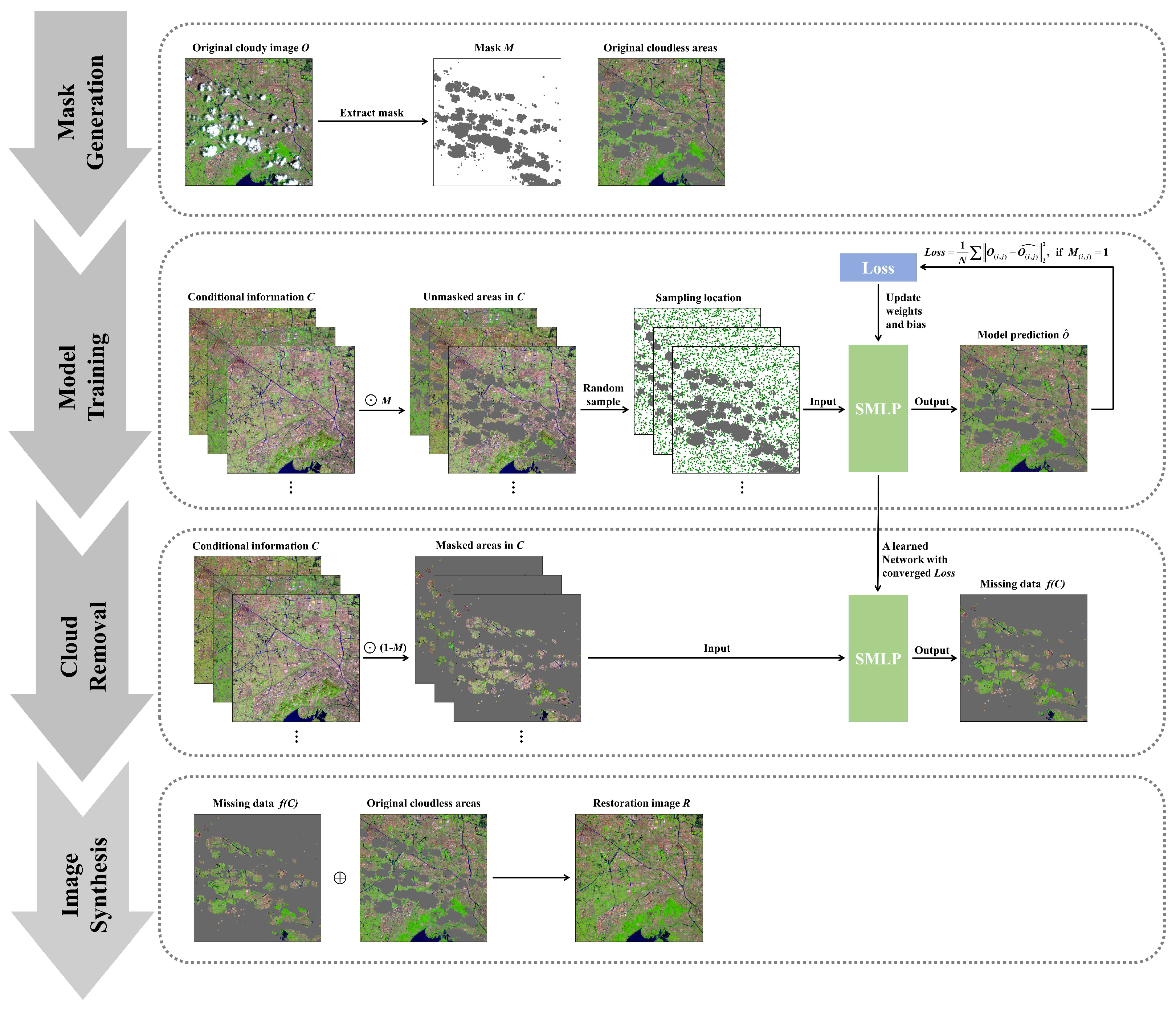
3.3. Cloud Removal Method Constrained by Conditional Information (SMLP-CR)

The SMLP-CR is shown in Figure 1.

3.3.1. Mask Generation

The article identifies cloud-covered areas using unsupervised classification. The method first classifies the cloudy RS image into several categories and then merges them by visual interpretation to generate the cloud mask. Afterward, the paper employs $3\times 3$ erosion and $7\times 7$ expansion for cloud-covered regions to eliminate tiny noise and to ensure that the mask covers all missing areas. At last, the cloudless sample areas and restoration areas are constructed by the mask.

3.3.2. Model Training

The paper defines the conditional information as $C\in {\mathbb{R}}^{w\times h\times c}$, where w, h, and c respectively represent the width, height, and number of channels of the conditional information. $O\in {\mathbb{R}}^{w\times h}$ denotes the original cloudy RS image. $R\in {\mathbb{R}}^{w\times h}$ is the cloud-free image after restoration. The cloud mask $M\in {\mathbb{R}}^{w\times h}$ is defined as:

$$M_{(i,j)}=\left\{\begin{array}{c}0,if(i,j)iscloud;\hfill \\ 1,otherwise.\hfill \end{array}\right.$$

(1)

In this paper, training samples are randomly collected in the cloudless area $(i,j)\in \left\{(x,y)\right|M_{(x,y)}=1\}$ of the original cloudy RS image. The mapping f is built based on SMLP, taking multisource conditional information C as inputs and the original image O as the expected output. The mapping f is calculated as follows:

$$\widehat{O_{(i,j)}}=f\left(C_{\left(i,j\right)}\right),if{M}_{(i,j)}=1.$$

(2)

The model chooses the mean square error (MSE) as the loss function $Loss$ and uses a backpropagation algorithm to train the model parameters. $Loss$ is obtained as:

$$Loss={\displaystyle \frac{1}{N}}\sum {∥O_{(i,j)}-\widehat{O_{(i,j)}}∥}_2^2,if{M}_{(i,j)}=1.$$

(3)

3.3.3. Cloud Removal

After model training, the method inputs conditional information C of the missing regions $(i,j)\in \left\{(x,y)\right|M_{(x,y)}=0\}$ into the model to obtain the missing data $f\left(C\right)$.

3.3.4. Image Synthesis

The article synthesizes the original undamaged regions with the restoration results of the missing regions and finally generates the restoration RS image R as follows:

$$R_{(i,j)}=\left\{\begin{array}{c}{O}_{(i,j)},if M_{(i,j)}=1;\hfill \\ f\left(C_{(i,j)}\right),if M_{(i,j)}=0.\hfill \end{array}\right.$$

(4)

4. Experiments

4.1. Datasets

4.1.1. Data Sources

There are often various ground objects in RS images. To validate the universality of our method, Suzhou (vegetation-dominated area), Kuqa (bare-land-dominated area), and Guangzhou (urban-dominated area) in China are selected as study areas. Two common RS satellite sensors (Landsat 8-9 OLI-TIRS and Sentinel-2 MSI) are applied for the experiments. Each area is divided into an application area, a simulation area, and a training area for the deep-learning methods (Figure 2). The experiments choose the shortwave infrared band (SWIR), the near-infrared band (NIR), and the red band (RED) as examples for restoration, which are often used in RS false-color composites. The details of the datasets can be seen in

Table 1. The description of the datasets.

Dataset	Data Source	Path/Row	Date of Restoration Images	Date of Conditional Images	Cloud-Covered Percentage of Applications/Simulations
Suzhou	Landsat 8-9 OLI-TIRS	119/038	18 June 2022	9 November 2021, 26 February 2022, 28 May 2023	43.2%/48.8%
Kuqa	Landsat 8-9 OLI-TIRS	145/031	1 October 2023	4 February 2022, 17 December 2022, 2 January 2023	33.5%/34.4%
Guangzhou	Sentinel-2 MSI	N0400/R089/T51STR	23 February 2023	16 October 2023, 20 November 2023, 25 December 2023	27.7%/22.0%

Cloud removal based on single-temporal conditional information utilizes the images from the bold date, for which the season is the same as that of the restoration images.

.

4.1.2. Data Preprocessing

Unlike deep-learning methods, SMLP-CR samples 100,000 pixels randomly at cloudless pixels in the simulation area or the experiment area as the training dataset and 10,000 pixels as the validation dataset. For the deep-learning methods in the comparison experiments, the paper crops the cloud-free training area to $64\times 64$ pixels then randomly divides them into training and validation datasets at a ratio of $4:1$.

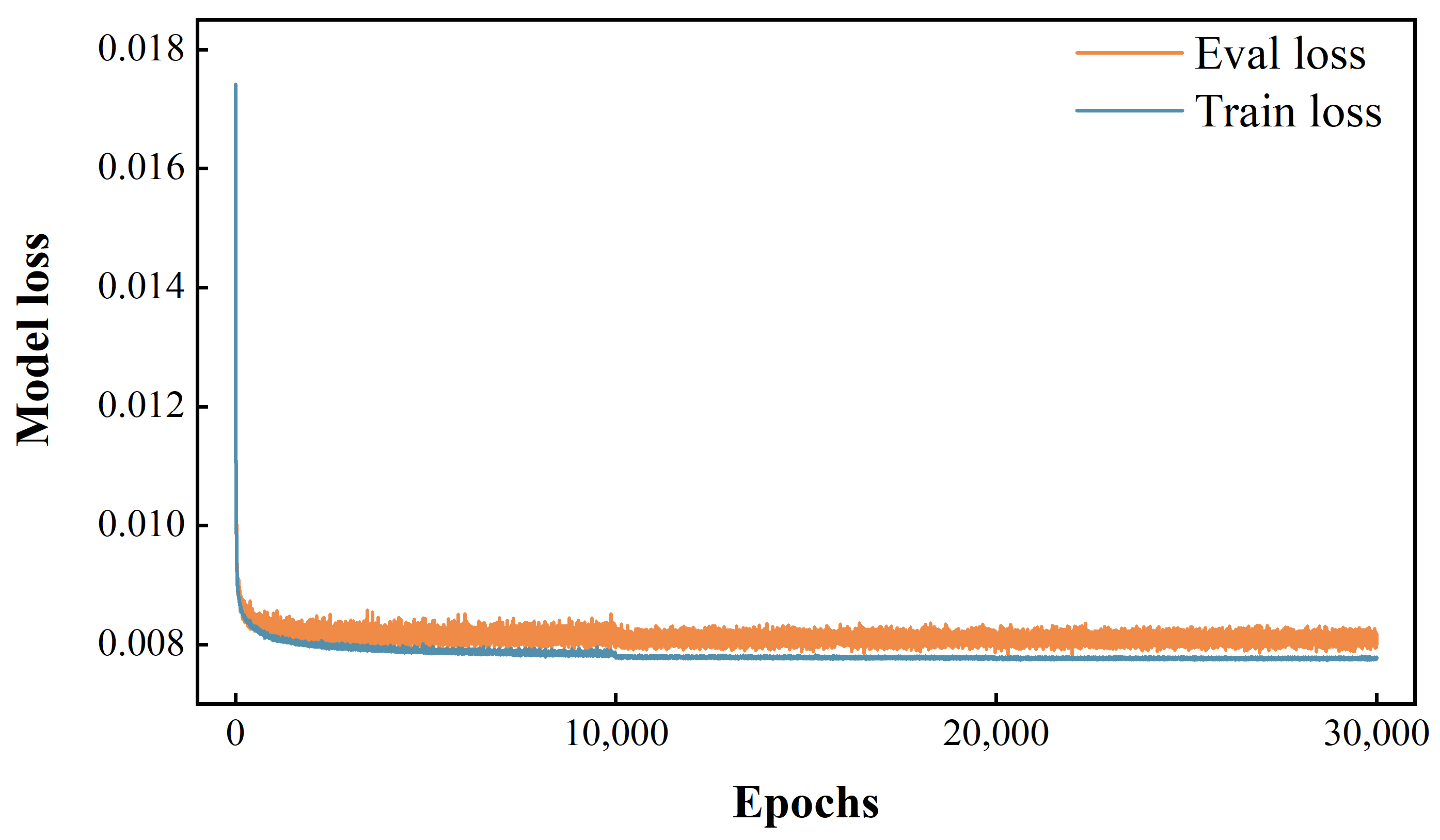
4.2. Evaluation Metrics and Implementation Details

The structure similarity (SSIM) [50] and peak signal–noise ratio (PSNR) are selected to measure the restoration results. For both metrics, higher values correspond to better results.

The number of types k for pixel similarity is set to 10. The batch size and learning rate of SMLP-CR are set as 4096 and 0.001, respectively. After every 10,000 iterations, the learning rate is multiplied by a weight decay of 0.1. The training process has 30,000 iterations. The Adam optimization algorithm is adopted to optimize the parameters. For instance, the input features of single-temporal Landsat 8 OLI-TIRS satellite images contain B1 to B7, B10, and B11 (nine channels), mean filtering of these bands adds 18 channels, and pixel similarity features after one-hot encoding include 10 channels, for a total of 37 input neurons. The output features are pixel values of specific bands of the restoration image, and there are three output neurons. The number of hidden layer neurons is set to 50.

4.3. Simulated Experiments using Various Temporal RS Images

The simulation area of the Suzhou dataset is restored by various temporal conditional information, and the results are displayed in

Table 2. Quantitative evaluation of simulation results for different temporal conditional information.

Conditional Information	SSIM↑			PSNR↓
	SWIR	NIR	RED	SWIR	NIR	RED
OLI-20211109	0.9147	0.9196	0.9650	39.11	38.91	44.31
OLI-20220226	0.9178	0.9038	0.9687	39.58	38.66	44.81
OLI-20230528	0.9271	0.9302	0.9713	40.17	39.84	45.25
MSI-20220227	0.8942	0.8812	0.9611	38.31	37.91	43.98
Multi-Temporal	0.9380	0.9458	0.9765	40.79	40.67	46.05

. To evaluate the restoration performance for heterogeneous images, Sentinel-2 MSI conditional images dated 27 July 2022 are added into the original Suzhou dataset. Among single-temporal conditional images, OLI-20230528, which is one year apart but in the same season as the restoration images, shows the best restoration results. This suggests that regular seasonal changes to ground objects have a greater impact on the restoration results than sudden shifts to ground objects over a year. The results for OLI-20220226 are slightly better than those for OLI-20211109, which is consistent with the general perception of researchers that the closer the temporal distance between conditional information and restoration images, the better the restoration results when regular seasonal variations to ground objects are excluded. Although MSI-20220227 is also close in temporal distance, it is taken by a different sensor with different wavelengths from the restoration images, so it is not restored very well. The loss curve for the SMLP-CR based on OLI-20230528 is shown in Figure 3. The training loss and validation loss are remarkably close and converge simultaneously, indicating excellent generalization.

All conditional information is input to the model, and the results using multi-temporal conditional information are significantly better than those for each set of single-temporal conditional information (Table 2). The restoration model based on multi-temporal conditional information is more likely to find nonlinear relationships between conditional information and restoration images; hence, it can predict sudden shifts and regular seasonal changes to ground objects and then achieves optimal performance. Meanwhile, the paper outputs feature importance based on the presingle-connection layer (

Table 3. Normalized feature importance measure of SMLP-CR for multi-temporal conditional information.

Conditional Information	OLI-20211109	OLI-20220226	OLI-20230528	MSI-20220227
Feature Importance	0.25	0.28	0.30	0.17

The feature importance of each single-temporal conditional information source is the sum of each input feature’s importance for those single-temporal images.

). The feature importance indicates that OLI-20230528 is the most important source for restoration, OLI-20220226 and OLI-20211109 are the next most important in order, and MSI-20220227 is the least important. The feature importance results can be effectively validated through the quantitative comparison of single-temporal conditional information in Table 2. As a result, SMLP-CR helps researchers understand how multisource conditional information affects the reconstruction results, enhancing the interpretability of the method. In general, the priority of conditional images for the cloud removal task should be homologous images, images from the same season, and images with close temporal distances.

4.4. Comparison Experiments and Discussions

4.4.1. Comparison Methods and Hyperparameters

Seven popular cloud removal methods are utilized as comparison methods, including a spatial-based method: GAN [28], a temporal-based method: LLHM [33], and six hybrid-based methods: STS-CNN [23], STGAN [12], SEN12MS-CR [15], CTGAN [14], PMAA [42], and DiffCR [8].

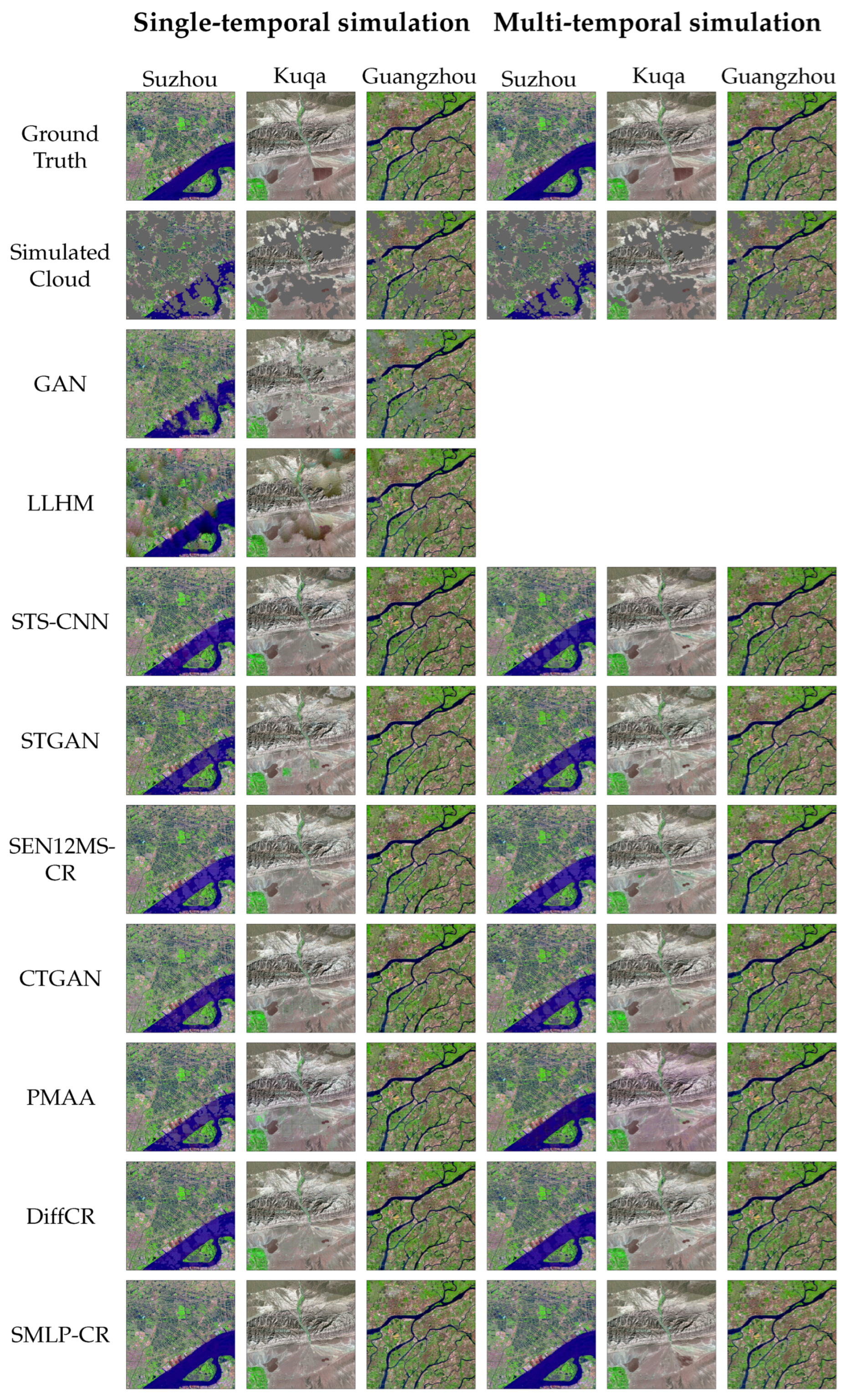
4.4.2. Simulated Comparison Experiments

Firstly, the missing regions in the simulation area are restored by single-temporal conditional information, for which the restoration results are exhibited in Figure 4, and the quantitative evaluation is shown in

Table 4. Quantitative comparison of simulated restorations based on single-temporal conditional information.

Method	Dataset
	Suzhou						Kuqa						Guangzhou
	SSIM			PSNR			SSIM			PSNR			SSIM			PSNR
	SWIR	NIR	RED	SWIR	NIR	RED	SWIR	NIR	RED	SWIR	NIR	RED	SWIR	NIR	RED	SWIR	NIR	RED
GAN (TGRS, 2021) [28]	0.7442	0.7237	0.8948	34.51	34.19	38.85	0.8751	0.8825	0.9079	46.06	46.04	46.97	0.8440	0.8506	0.8696	45.60	45.59	45.60
LLHM (USGS, 2005) [33]	0.8871	0.8582	0.9546	36.97	36.03	40.67	0.9642	0.9620	0.9681	50.01	49.85	50.74	0.9558	0.9498	0.9562	47.75	47.78	49.33
STS-CNN (TGRS, 2018) [23]	0.9207	0.9233	0.9665	38.38	37.99	43.36	0.9754	0.9742	0.9811	50.88	51.07	52.17	0.9681	0.9601	0.9628	49.37	48.80	49.96
STGAN (WACV, 2020) [12]	0.8596	0.8474	0.9369	35.91	35.19	40.35	0.9598	0.9571	0.9671	47.89	47.35	48.68	0.9560	0.9438	0.9446	47.69	47.32	48.13
SEN12MS-CR (TGRS, 2022) [15]	0.8953	0.8935	0.9512	37.18	36.64	41.18	0.9700	0.9669	0.9751	49.93	49.58	50.95	0.9623	0.9477	0.9496	48.47	47.70	48.61
CTGAN (ICIP, 2022) [14]	0.8747	0.8868	0.9443	36.65	35.98	41.83	0.9710	0.9693	0.9760	49.66	49.58	50.59	0.9663	0.9535	0.9562	48.62	48.03	48.79
PMAA (ECAI, 2023) [42]	0.8981	0.9036	0.9580	37.11	36.65	42.60	0.9752	0.9710	0.9790	50.13	48.62	50.82	0.9660	0.9507	0.9564	48.82	47.95	49.30
DiffCR (TGRS, 2024) [8]	0.9109	0.9153	0.9549	38.22	37.75	42.04	0.9731	0.9703	0.9758	50.53	49.86	51.01	0.9658	0.9542	0.9539	48.68	48.05	48.55
SMLP-CR	0.9266	0.9307	0.9710	40.19	39.88	45.18	0.9804	0.9786	0.9843	53.00	52.90	54.45	0.9694	0.9614	0.9653	49.23	48.82	50.11

The bold values indicate the best performance among these methods.

. The selection of single-temporal conditional information can be seen in the footnote of Table 1. GANs do not require the involvement of conditional information, boasting broader applicability, but it is obvious that the performance of GANs is relatively poor, and GANs produce extensive artifacts. The results of LLHM demonstrate texture discontinuity or spectral distortion to some degree, especially in land areas with complex textures, which illustrates that the relationships among various temporal data are not easy linear correlations but are extremely complex nonlinear correlations. CGAN-based methods—STGAN, SEN12MS-CR, CTGAN, and PMAA—prioritize multi-temporal information; thus, their performance is limited for single-temporal conditional information. Compared to these CGAN models, DiffCR is more stable and exhibits superior restoration results. STS-CNN stands out as the top-performing deep-learning method. However, all of the deep-learning methods tend to generate blurry details in cloud-covered areas, resulting in some degree of distortion. Moreover, these methods display noticeable artifacts when restoring smooth-textured water. In contrast, SMLP-CR reconstructs cloud-covered areas with better detail restoration and less spectral distortion based on multi-scale local information. SMLP-CR also displays the best performance in the quantitative evaluation.

Except for GAN and LLHM, the other methods all satisfy the input of multi-temporal conditional information. STS-CNN simply concatenates multi-temporal conditional images along the channel dimension and inputs them into the CNN, leading to a slight improvement in restoration performance. STGAN concatenates multi-temporal images in pairs, SEN12MS-CR integrates multi-temporal condition information using 3-D convolutions, CTGAN utilizes a transformer to establish long-term dependencies in multi-temporal condition information, PMAA introduces a novel multi-scale attention module to establish the long-range dependencies of multi-temporal features, and DiffCR employs a condition encoder to fuse multi-temporal condition information. Therefore, the inclusion of multi-temporal condition information significantly enhances the performance of these deep-learning methods. Even with performance improvements, these deep-learning algorithms still cannot solve the problem of artifacts in water (Figure 4). SMLP-CR integrates hybrid information that enables it to sample directly in the vicinity of clouds. Its quantitative metrics still outperform deep-learning methods in the simulation of multi-temporal conditional information, with an average improvement to the SSIM and PSNR of 0.0058 and 2.00, respectively, compared with STS-CNN (

Table 5. Quantitative comparison of simulated restorations based on multi-temporal conditional information.

Method	Dataset
	Suzhou						Kuqa						Guangzhou
	SSIM			PSNR			SSIM			PSNR			SSIM			PSNR
	SWIR	NIR	RED	SWIR	NIR	RED	SWIR	NIR	RED	SWIR	NIR	RED	SWIR	NIR	RED	SWIR	NIR	RED
STS-CNN (TGRS, 2018)	0.9289	0.9306	0.9718	38.91	37.98	43.80	0.9809	0.9800	0.9852	51.98	52.66	53.44	0.9737	0.9695	0.9701	50.18	49.84	50.93
STGAN (WACV, 2020)	0.9023	0.9043	0.9596	37.01	36.40	41.64	0.9687	0.9647	0.9744	49.04	48.17	49.94	0.9660	0.9611	0.9610	48.25	48.18	49.21
SEN12MS-CR (TGRS, 2022)	0.9157	0.9242	0.9664	38.23	37.79	42.58	0.9756	0.9734	0.9797	51.79	51.51	52.56	0.9756	0.9648	0.9695	50.01	49.00	50.45
CTGAN (ICIP, 2022)	0.9040	0.9120	0.9586	37.51	37.04	42.24	0.9751	0.9730	0.9797	50.88	50.54	51.69	0.9722	0.9672	0.9690	49.12	48.86	50.14
PMAA (ECAI, 2023)	0.9188	0.9315	0.9651	39.22	38.82	42.44	0.9792	0.9781	0.9834	51.66	51.96	52.13	0.9726	0.9695	0.9729	49.76	49.50	51.13
DiffCR (TGRS, 2024)	0.9180	0.9288	0.9608	38.64	38.45	42.62	0.9765	0.9737	0.9790	51.95	51.03	51.77	0.9753	0.9686	0.9706	50.08	49.53	50.65
SMLP-CR	0.9363	0.9449	0.9753	40.76	40.74	45.98	0.9848	0.9834	0.9882	55.16	55.06	56.59	0.9779	0.9745	0.9773	50.85	50.54	52.11

The bold values indicate the best performance among these methods.

).

Finally, the computational times and the numbers of parameters of these deep-learning methods and SMLP-CR are exhibited in

Table 6. The model complexities of various deep-learning methods and SMLP-CR.

Method	Model Complexity
	Floating Point Operations (FLOPs)	Parameters
STS-CNN (TGRS, 2018)	$3.03\times {10}^{12}$	$3.19\times {10}^5$
STGAN (WACV, 2020)	$9.46\times {10}^{12}$	$1.42\times {10}^7$
SEN12MS-CR (TGRS, 2022)	$1.11\times {10}^{15}$	$4.15\times {10}^7$
CTGAN (ICIP, 2022)	$5.36\times {10}^{13}$	$2.50\times {10}^7$
PMAA (ECAI, 2023)	$1.37\times {10}^{13}$	$6.32\times {10}^6$
DiffCR (TGRS, 2024)	$4.23\times {10}^{12}$	$2.29\times {10}^7$
SMLP-CR	$5.81\times {10}^8$	$5.86\times {10}^3$

FLOPs measure the number of floating point calculations for forward propagation of the model, which represent the time complexity.

. It is evident that the lighter-weight SMLP-CR has the advantages of fewer parameters and faster computation speed.

SMLP-CR requires cloud-free conditional images. The short revisit periods of RS satellites enable multiple repeated captures of a specific area. The revisit periods of common satellites like Landsat 8 and Sentinel-2 are 16 days and 5 days, respectively, so obtaining cloud-free conditional images is relatively straightforward. Even if there are a few clouds in conditional images, as long as the clouds in the conditional images and those in the restoration image do not overlap, SMLP-CR can still sample at cloud-free pixels in both images to complete the cloud removal task. In general, the demands of our method for conditional images are easily met.

4.4.3. Real-World Comparison Experiments

The reconstruction of cloud-covered areas in the application area is shown in Figure 5. There is significant spectral distortion in the restoration results of GAN and LLHM. Further, it can be seen in the Suzhou dataset that deep-learning methods produce purple artifacts when reconstructing water pixels, but the result of SMLP-CR exhibits lower spectral distortion. For the Kuqa dataset, SMLP-CR demonstrates notably superior color consistency in the oasis through the details of Figure 5. Comparative methods show varying degrees of texture discontinuity in the details of Figure 5 when restoring images form the Guangzhou dataset. In contrast, SMLP-CR demonstrates stronger texture continuity. Therefore, SMLP-CR performs better at reducing spectral distortion, maintaining color consistency, ensuring texture continuity, and restoring image details.

5. Conclusions

SMLP-CR is a lightweight cloud removal method for RS images based on conditional information. It obtains spatial information through multi-scale mean filtering and local neighborhood sampling. Spectral and temporal information is acquired by multiple bands and multi-temporal RS images. It also applies unsupervised classification to find obviously simple relationships among similar pixels. The model employs SMLP networks to reconstruct missing regions covered by clouds on the basis of this multisource conditional information. The SMLP network not only improves the interpretability of the model but also finds the best way to select conditional information through its feature importance measure—homologous images first, images of the same season as the restoration image second, and finally, images with close temporal distances.

Compared with traditional methods, SMLP-CR can better fit complex nonlinear relationships. Instead of the demand for large cloud-free training areas and massive computing resources as required by deep-learning methods, SMLP-CR directly samples in neighborhoods of missing areas and has lower model complexity, facilitating the model finding the optimal mapping. Comparative experiments demonstrate that SMLP-CR not only performs better in qualitative comparisons such as visual consistency and texture continuity, but it also shows apparent advantages in the quantitative metrics. Compared to STS-CNN, SMLP-CR achieves average improvements of 0.0058 to the SSIM and 2.00 to the PSNR.

The conditional images for SMLP-CR are expected to be cloud-free; this requirement will be easily met since the satellite revisit period is extremely short and there will be a huge number of reference RS images. However, the performance of SMLP-CR may be limited in areas where reference RS images are scarce. In general, SMLP-CR is suitable for a variety of application scenarios, enhancing the utilization of RS data and expanding the range of applications. In the future, SMLP-CR may be employed for reconstructing various types of missing data in RS fields, such as super-resolution reconstruction of RS images.

References

1. Guo, H.; Shi, Q.; Marinoni, A.; Du, B.; Zhang, L. Deep Building Footprint Update Network: A Semi-Supervised Method for Updating Existing Building Footprint from Bi-Temporal Remote Sensing Images. Remote Sens. Environ. 2021, 264, 112589. [Google Scholar] [CrossRef]
2. He, D.; Shi, Q.; Liu, X.; Zhong, Y.; Zhang, X. Deep Subpixel Mapping Based on Semantic Information Modulated Network for Urban Land Use Mapping. IEEE Trans. Geosci. Remote Sens. 2021, 59, 10628–10646. [Google Scholar] [CrossRef]
3. He, L.; Qi, S.L.; Duan, L.Z.; Guo, T.C.; Feng, W.; He, D.X. Monitoring of Wheat Powdery Mildew Disease Severity Using Multiangle Hyperspectral Remote Sensing. IEEE Trans. Geosci. Remote Sens. 2021, 59, 979–990. [Google Scholar] [CrossRef]
4. Weiss, M.; Jacob, F.; Duveiller, G. Remote Sensing for Agricultural Applications: A Meta-Review. Remote Sens. Environ. 2020, 236, 111402. [Google Scholar] [CrossRef]
5. Maheswaran, G.; Selvarani, A.G.; Elangovan, K. Groundwater Resource Exploration in Salem District, Tamil Nadu Using GIS and Remote Sensing. J. Earth Syst. Sci. 2016, 125, 311–328. [Google Scholar] [CrossRef]
6. Shirmard, H.; Farahbakhsh, E.; Müller, R.D.; Chandra, R. A Review of Machine Learning in Processing Remote Sensing Data for Mineral Exploration. Remote Sens. Environ. 2022, 268, 112750. [Google Scholar] [CrossRef]
7. Mao, K.; Yuan, Z.; Zuo, Z.; Xu, T.; Shen, X.; Gao, C. Changes in Global Cloud Cover Based on Remote Sensing Data from 2003 to 2012. Chin. Geogr. Sci. 2019, 29, 306–315. [Google Scholar] [CrossRef]
8. Zou, X.; Li, K.; Xing, J.; Zhang, Y.; Wang, S.; Jin, L.; Tao, P. DiffCR: A Fast Conditional Diffusion Framework for Cloud Removal from Optical Satellite Images. IEEE Trans. Geosci. Remote Sens. 2024, 62, 1–14. [Google Scholar] [CrossRef]
9. Jiang, B.; Li, X.; Chong, H.; Wu, Y.; Li, Y.; Jia, J.; Wang, S.; Wang, J.; Chen, X. A Deep-Learning Reconstruction Method for Remote Sensing Images with Large Thick Cloud Cover. Int. J. Appl. Earth Obs. Geoinf. 2022, 115, 103079. [Google Scholar] [CrossRef]
10. Li, W.; Li, Y.; Chen, D.; Chan, J.C.W. Thin Cloud Removal with Residual Symmetrical Concatenation Network. ISPRS J. Photogramm. Remote Sens. 2019, 153, 137–150. [Google Scholar] [CrossRef]
11. Zhang, Q.; Yuan, Q.; Li, J.; Li, Z.; Shen, H.; Zhang, L. Thick Cloud and Cloud Shadow Removal in Multitemporal Imagery Using Progressively Spatio-Temporal Patch Group Deep Learning. ISPRS J. Photogramm. Remote Sens. 2020, 162, 148–160. [Google Scholar] [CrossRef]
12. Sarukkai, V.; Jain, A.; Uzkent, B.; Ermon, S. Cloud Removal in Satellite Images Using Spatiotemporal Generative Networks. In Proceedings of the 2020 IEEE Winter Conference on Applications of Computer Vision (WACV), Snowmass Village, CO, USA, 1–5 March 2020; pp. 1785–1794. [Google Scholar] [CrossRef]
13. Long, C.; Yang, J.; Guan, X.; Li, X. Thick Cloud Removal from Remote Sensing Images Using Double Shift Networks. In Proceedings of the 2021 IEEE International Geoscience and Remote Sensing Symposium IGARSS, Brussels, Belgium, 11–16 July 2021; pp. 2687–2690. [Google Scholar] [CrossRef]
14. Huang, G.L.; Wu, P.Y. CTGAN: Cloud Transformer Generative Adversarial Network. In Proceedings of the 2022 IEEE International Conference on Image Processing (ICIP), Bordeaux, France, 16–19 October 2022; pp. 511–515. [Google Scholar] [CrossRef]
15. Ebel, P.; Xu, Y.; Schmitt, M.; Zhu, X.X. SEN12MS-CR-TS: A Remote-Sensing Data Set for Multimodal Multitemporal Cloud Removal. IEEE Trans. Geosci. Remote Sens. 2022, 60, 1–14. [Google Scholar] [CrossRef]
16. Gao, J.; Yuan, Q.; Li, J.; Su, X. Unsupervised Missing Information Reconstruction for Single Remote Sensing Image with Deep Code Regression. Int. J. Appl. Earth Obs. Geoinf. 2021, 105, 102599. [Google Scholar] [CrossRef]
17. Liu, W.; Jiang, Y.; Li, F.; Zhang, G.; Song, H.; Wang, C.; Li, X. Collaborative Dual-Harmonization Reconstruction Network for Large-Ratio Cloud Occlusion Missing Information in High-Resolution Remote Sensing Images. Eng. Appl. Artif. Intell. 2024, 136, 108861. [Google Scholar] [CrossRef]
18. Li, J.; Hassani, A.; Walton, S.; Shi, H. ConvMLP: Hierarchical Convolutional MLPs for Vision. In Proceedings of the 2023 IEEE/CVF Conference on Computer Vision and Pattern Recognition Workshops (CVPRW), Vancouver, BC, Canada, 17–24 June 2023; pp. 6307–6316. [Google Scholar] [CrossRef]
19. Tolstikhin, I.; Houlsby, N.; Kolesnikov, A.; Beyer, L.; Zhai, X.; Unterthiner, T.; Yung, J.; Steiner, A.; Keysers, D.; Uszkoreit, J.; et al. MLP-Mixer: An All-MLP Architecture for Vision. arXiv 2021, arXiv:2105.01601. [Google Scholar]
20. Wang, Y.; Tang, S.; Zhu, F.; Bai, L.; Zhao, R.; Qi, D.; Ouyang, W. Revisiting the Transferability of Supervised Pretraining: An MLP Perspective. arXiv 2022, arXiv:2112.00496. [Google Scholar] [CrossRef]
21. Bozic, V.; Dordevic, D.; Coppola, D.; Thommes, J.; Singh, S.P. Rethinking Attention: Exploring Shallow Feed-Forward Neural Networks as an Alternative to Attention Layers in Transformers. arXiv 2024, arXiv:2311.10642. [Google Scholar] [CrossRef]
22. Tobler, W.R. A Computer Movie Simulating Urban Growth in the Detroit Region. Econ. Geogr. 1970, 46, 234–240. [Google Scholar] [CrossRef]
23. Zhang, Q.; Yuan, Q.; Zeng, C.; Li, X.; Wei, Y. Missing Data Reconstruction in Remote Sensing Image with a Unified Spatial–Temporal–Spectral Deep Convolutional Neural Network. IEEE Trans. Geosci. Remote Sens. 2018, 56, 4274–4288. [Google Scholar] [CrossRef]
24. Chen, Y.; Nan, Z.; Cao, Z.; Ou, M.; Feng, K. A Stepwise Framework for Interpolating Land Surface Temperature under Cloudy Conditions Based on the Solar-Cloud-Satellite Geometry. ISPRS J. Photogramm. Remote Sens. 2023, 197, 292–308. [Google Scholar] [CrossRef]
25. Shi, C.; Wang, T.; Wang, S.; Jia, A.; Zheng, X.; Leng, W.; Du, Y. MDINEOF: A Scheme to Recover Land Surface Temperatures under Cloudy-Sky Conditions by Incorporating Radiation Fluxes. Remote Sens. Environ. 2024, 309, 114208. [Google Scholar] [CrossRef]
26. Jing, R.; Duan, F.; Lu, F.; Zhang, M.; Zhao, W. Denoising Diffusion Probabilistic Feature-Based Network for Cloud Removal in Sentinel-2 Imagery. Remote Sens. 2023, 15, 2217. [Google Scholar] [CrossRef]
27. Chen, Y.; He, W.; Yokoya, N.; Huang, T.Z. Blind Cloud and Cloud Shadow Removal of Multitemporal Images Based on Total Variation Regularized Low-Rank Sparsity Decomposition. ISPRS J. Photogramm. Remote Sens. 2019, 157, 93–107. [Google Scholar] [CrossRef]
28. Zheng, J.; Liu, X.Y.; Wang, X. Single Image Cloud Removal Using U-Net and Generative Adversarial Networks. IEEE Trans. Geosci. Remote Sens. 2021, 59, 6371–6385. [Google Scholar] [CrossRef]
29. Pan, H. Cloud Removal for Remote Sensing Imagery via Spatial Attention Generative Adversarial Network. arXiv 2020, arXiv:2009.13015. [Google Scholar] [CrossRef]
30. Sui, J.; Ma, Y.; Yang, W.; Zhang, X.; Pun, M.O.; Liu, J. Diffusion Enhancement for Cloud Removal in Ultra-Resolution Remote Sensing Imagery. IEEE Trans. Geosci. Remote Sens. 2024, 62, 1–14. [Google Scholar] [CrossRef]
31. Wang, L.; Qu, J.; Xiong, X.; Hao, X.; Xie, Y.; Che, N. A New Method for Retrieving Band 6 of Aqua MODIS. IEEE Geosci. Remote Sens. Lett. 2006, 3, 267–270. [Google Scholar] [CrossRef]
32. Rakwatin, P.; Takeuchi, W.; Yasuoka, Y. Restoration of Aqua MODIS Band 6 Using Histogram Matching and Local Least Squares Fitting. IEEE Trans. Geosci. Remote Sens. 2009, 47, 613–627. [Google Scholar] [CrossRef]
33. Storey, J.; Scaramuzza, P.; Schmidt, G.; Barsi, J. Landsat 7 Scan Line Corrector-off Gap-Filled Product Development. In Proceedings of the Pecora 16 “Global Priorities in Land Remote Sensing”, Sioux Falls, South Dakota, 23–27 October 2005. [Google Scholar]
34. Zeng, C.; Shen, H.; Zhang, L. Recovering Missing Pixels for Landsat ETM+ SLC-off Imagery Using Multi-Temporal Regression Analysis and a Regularization Method. Remote Sens. Environ. 2013, 131, 182–194. [Google Scholar] [CrossRef]
35. Li, X.; Shen, H.; Li, H.; Zhang, L. Patch Matching-Based Multitemporal Group Sparse Representation for the Missing Information Reconstruction of Remote-Sensing Images. IEEE J. Sel. Top. Appl. Earth Obs. Remote Sens. 2016, 9, 3629–3641. [Google Scholar] [CrossRef]
36. Ng, M.K.P.; Yuan, Q.; Yan, L.; Sun, J. An Adaptive Weighted Tensor Completion Method for the Recovery of Remote Sensing Images with Missing Data. IEEE Trans. Geosci. Remote Sens. 2017, 55, 3367–3381. [Google Scholar] [CrossRef]
37. Sun, D.L.; Ji, T.Y.; Ding, M. A New Sparse Collaborative Low-Rank Prior Knowledge Representation for Thick Cloud Removal in Remote Sensing Images. Remote Sens. 2024, 16, 1518. [Google Scholar] [CrossRef]
38. Isola, P.; Zhu, J.Y.; Zhou, T.; Efros, A.A. Image-to-Image Translation with Conditional Adversarial Networks. arXiv 2018, arXiv:1611.07004. [Google Scholar] [CrossRef]
39. Liu, H.; Huang, B.; Cai, J. Thick Cloud Removal Under Land Cover Changes Using Multisource Satellite Imagery and a Spatiotemporal Attention Network. IEEE Trans. Geosci. Remote Sens. 2023, 61, 1–18. [Google Scholar] [CrossRef]
40. Garnot, V.S.F.; Landrieu, L. Lightweight Temporal Self-Attention for Classifying Satellite Image Time Series. arXiv 2020, arXiv:2007.00586. [Google Scholar] [CrossRef]
41. Ebel, P.; Garnot, V.S.F.; Schmitt, M.; Wegner, J.D.; Zhu, X.X. UnCRtainTS: Uncertainty Quantification for Cloud Removal in Optical Satellite Time Series. In Proceedings of the IEEE/CVF Conference on Computer Vision and Pattern Recognition, Vancouver, BC, Canada, 17–24 June 2023; pp. 2086–2096. [Google Scholar]
42. Zou, X.; Li, K.; Xing, J.; Tao, P.; Cui, Y. PMAA: A Progressive Multi-scale Attention Autoencoder Model for High-performance Cloud Removal from Multi-temporal Satellite Imagery. arXiv 2023, arXiv:2303.16565. [Google Scholar] [CrossRef]
43. Arjovsky, M.; Chintala, S.; Bottou, L. Wasserstein GAN. arXiv 2017, arXiv:1701.07875. [Google Scholar] [CrossRef]
44. Gulrajani, I.; Ahmed, F.; Arjovsky, M.; Dumoulin, V.; Courville, A.C. Improved Training of Wasserstein GANs. In Proceedings of the Advances in Neural Information Processing Systems, Long Beach, CA, USA, 4–9 December 2017. [Google Scholar]
45. Elfeki, M.; Couprie, C.; Riviere, M.; Elhoseiny, M. GDPP: Learning Diverse Generations Using Determinantal Point Processes. In Proceedings of the 36th International Conference on Machine Learning, Long Beach, CA, USA, 9–15 June 2019; pp. 1774–1783. [Google Scholar]
46. Zhang, W.; Shen, X.; Zhang, H.; Yin, Z.; Sun, J.; Zhang, X.; Zou, L. Feature Importance Measure of a Multilayer Perceptron Based on the Presingle-Connection Layer. Knowl. Inf. Syst. 2024, 66, 511–533. [Google Scholar] [CrossRef]
47. Stollfuss, B.; Bacher, M. MLP-Supported Mathematical Optimization of Simulation Models: Investigation into the Approximation of Black Box Functions of Any Simulation Model with MLPs with the Aim of Functional Analysis. In Proceedings of the 3rd International Conference on Innovative Intelligent Industrial Production and Logistics, Valletta, Malta, 24–26 October 2022; pp. 107–114. [Google Scholar] [CrossRef]
48. Mirza, M.; Osindero, S. Conditional Generative Adversarial Nets. arXiv 2014, arXiv:1411.1784. [Google Scholar]
49. Chen, T.J. A Novel Image Blurring Detection Scheme Using Spatial Autocorrelation. In Proceedings of the 2023 34th Irish Signals and Systems Conference (ISSC), Dublin, Ireland, 13–14 June 2023; pp. 1–4. [Google Scholar] [CrossRef]
50. Wang, Z.; Bovik, A.; Sheikh, H.; Simoncelli, E. Image Quality Assessment: From Error Visibility to Structural Similarity. IEEE Trans. Image Process. 2004, 13, 600–612. [Google Scholar] [CrossRef]
Figure 1. The flowchart of the cloud removal method constrained by conditional information (SMLP-CR).
Remotesensing 16 03134 g001
Figure 2. The presentation of the datasets. Box a is the application area. Box b represents the simulation area, and box c expresses the cloud-free training area for the deep-learning methods.
Remotesensing 16 03134 g002
Figure 3. The loss curve of SMLP-CR based on OLI-20230528.
Remotesensing 16 03134 g003
Figure 4. Simulation results of SMLP-CR and comparison methods. The results show false-color composite RS images using SWIR, NIR, and RED bands.
Remotesensing 16 03134 g004
Figure 5. Real-world restoration results of SMLP-CR and comparison methods. The results show false-color composite RS images using SWIR, NIR, and RED bands. Details of the restoration in the red box are shown in the upper-right enlarged image.
Remotesensing 16 03134 g005