Article

Weighted Variable Optimization-Based Method for Estimating Soil Salinity Using Multi-Source Remote Sensing Data: A Case Study in the Weiku Oasis, Xinjiang, China

1
College of Geography and Remote Sensing Sciences, Xinjiang University, Urumqi 830046, China
2
Institute for Beautiful China, Xinjiang University, Urumqi 830046, China
3
Xinjiang Uygur Autonomous Region Comprehensive Land Management Center, Urumqi 830063, China
4
Ministry of Natural Resources Desert-Oasis Ecological Monitoring and Restoration Engineering Technology Innovation Center, Urumqi 830063, China
5
Field Scientific Observatory for Soil and Water Processes and Ecological Security in Oasis of Tarim River Headwaters Area, Ministry of Natural Resources of China, Aksu 843000, China
6
Xinjiang Institute of Technology, Aksu 843100, China
*
Author to whom correspondence should be addressed.
These authors contributed equally to this work.
Remote Sens. 2024, 16(17), 3145; https://doi.org/10.3390/rs16173145
Submission received: 29 June 2024 / Revised: 16 August 2024 / Accepted: 22 August 2024 / Published: 26 August 2024

Abstract

:
Soil salinization is a significant global threat to sustainable agricultural development, with soil salinity serving as a crucial indicator for evaluating soil salinization. Remote sensing technology enables large-scale inversion of soil salinity, facilitating the monitoring and assessment of soil salinization levels, thus supporting the prevention and management of soil salinization. This study employs multi-source remote sensing data, selecting 8 radar polarization combinations, 10 spectral indices, and 3 topographic factors to form a feature variable dataset. By applying a normalized weighted variable optimization method, highly important feature variables are identified. AdaBoost, LightGBM, and CatBoost machine learning methods are then used to develop soil salinity inversion models and evaluate their performance. The results indicate the following: (1) There is generally a strong correlation between radar polarization combinations and vegetation indices, and a very high correlation between various vegetation indices and the salinity index S3. (2) The top five feature variables, in order of importance, are Aspect, VH2, Normalized Difference Moisture Index (NDMI), VH, and Vegetation Moisture Index (VMI). (3) The method of normalized weighted importance scoring effectively screens important variables, reducing the number of input feature variables while enhancing the model’s inversion accuracy. (4) Among the three machine learning models, CatBoost performs best overall in soil salt content (SSC) prediction. Combined with the top five feature variables, CatBoost achieves the highest prediction accuracy (R2 = 0.831, RMSE = 2.653, MAE = 1.034) in the prediction phase. This study provides insights for the further development and application of methods for collaborative inversion of soil salinity using multi-source remote sensing data.

1. Introduction

Soil salinization refers to the accumulation of soluble salts in the soil due to natural factors such as climate, hydrology, and topography, or due to destructive human activities combined with fragile ecological environments, leading to the degradation of soil quality and the formation of saline soil [1], severely impacting agricultural productivity and environmental sustainability [2]. It has a significant negative impact on the global economy, with annual global income losses reaching up to $27.3 billion [3]. Therefore, using scientific methods to accurately invert and monitor the dynamics of arable soil salinization, and to timely manage and mitigate soil salinization, is of great importance for regional food production and sustainable agricultural development.
Traditional salinization surveys require manual field soil sampling, which is time-consuming, labor-intensive, and costly, making it difficult to achieve large-scale or high-precision dynamic monitoring. This is especially challenging in areas with complex underlying surfaces and harsh natural environments, where monitoring stations are insufficient, and field surveys are difficult [4,5]. In contrast, remote sensing technology can observe specific areas and offers advantages such as rich information and wide monitoring coverage. Optical remote sensing can provide multi-band spectral information that is highly sensitive to soil salinity, allowing researchers to invert soil salinity by constructing spectral indices. Numerous studies have shown that combining Sentinel-2 data with machine learning methods can further explore the correlation between dependent variables and remote sensing images [6,7,8,9]. However, single optical data is easily affected by imaging time and weather conditions such as clouds and rain, and relying on spectral features to extract salinization information has limitations. Synthetic aperture radar (SAR) sensors, on the other hand, are less affected by weather conditions and can penetrate certain soil depths [10]; therefore, to improve monitoring accuracy, more and more studies are choosing to collaboratively invert soil salinity using optical and radar satellites [11,12,13]. Additionally, topographic factors play an important role in soil salinization by influencing water distribution and salt accumulation. Research has shown that areas with gentle slopes are more likely to accumulate salts, while in steeper areas, salts are often washed away [14]. Florinsky [15] found that south-facing slopes usually have higher soil salinity compared to north-facing slopes. Bannari et al. [16] demonstrated a significant negative correlation between elevation and soil salinity, with higher elevations having lower soil salinity. Thus, in addition to optical and radar satellite data, this study also includes elevation, aspect, and slope as feature variables.
The causes of soil salinization and the composition of soil salts are complex, and there are differences in the selection of feature variables in different regions [17]. Therefore, different methods are needed to select characteristic variables for constructing inversion models. Research indicates that random forest classification, recursive feature elimination (RFE), and partial least squares variable importance projection (PLS-VIP) methods show significant advantages in the inversion of soil salinity and other physicochemical properties. Using the random forest classification method combined with Sentinel-2 data can effectively enhance the capability to monitor soil salinization under data-scarce conditions [18]. The RFE method, combined with random forest (RF) and support vector regression (SVR) models, can improve the accuracy of soil pH prediction [19]. The PLS-VIP method for selecting characteristic bands, combined with competitive adaptive reweighted sampling (CARS), can significantly enhance the inversion accuracy of soil moisture and salinity information [20]. The integration of variable selection methods with machine learning algorithms for soil salinity inversion has been a research focus in recent years. However, the process of selecting characteristic variables is complex and subjective, and there is no comprehensive and suitable standard for the selection method and threshold determination of characteristic variables. This study proposes a normalized weighted importance scoring method for importance ranking. Based on this ranking, different combinations of variables are selected and combined with machine learning models to determine the most suitable variables and models for soil salinity inversion in the study area.
Machine learning is playing an increasingly important role in the inversion of soil salinity content. Traditional methods rely on time-consuming and labor-intensive ground measurements, whereas machine learning algorithms can handle large-scale, multidimensional data, providing more efficient and accurate inversion results. Studies have shown that combining multi-source remote sensing data with machine learning algorithms, such as support vector machines (SVM), extreme learning machines (ELM), and RF, can significantly improve the accuracy of soil salinity inversion [21,22]. Gradient boosting models like LightGBM have demonstrated significant advantages in soil salinization monitoring due to their powerful feature selection capabilities and high computational efficiency. In soil electrical conductivity inversion studies, the use of LightGBM, combined with various spectral preprocessing methods, significantly enhanced the model’s predictive accuracy [23]. LightGBM also showed superior adaptability and computational efficiency in soil salinity inversion in the coastal cotton-growing regions of South Kazakhstan and China, achieving excellent predictive results [24,25]. Although there are no specific studies on the application of AdaBoost in soil salinity content inversion, this gradient boosting model has demonstrated significant performance in other environmental variable prediction tasks, such as soil organic matter content inversion [26]. CatBoost, another new boosting algorithm, excels in handling categorical features and small sample data. For example, in soil moisture prediction, CatBoost exhibited higher predictive accuracy and lower error on small sample data compared to LightGBM. In soil moisture prediction, the mean absolute error (MAE) was 2.40%, indicating high predictive accuracy [27]. While CatBoost has shown excellent performance in predicting other environmental parameters, it has not yet been widely applied to soil salinity content inversion. Thus, adopting the CatBoost model holds potential for improving the accuracy of soil salinity content estimation.
The Weiku Oasis is a typical irrigated oasis in Xinjiang, China, and one of the core areas for economic development in southern Xinjiang. The Weiku Oasis has large-scale salt deposits and widespread soil salinization, posing a serious threat to its development. Therefore, this study selects the Weiku Oasis as the research area using a feature variable dataset composed of 8 radar polarization combinations, 10 multispectral indices, and 3 topographic factors. By applying a normalized weighted importance scoring method, the variables that contribute most to the model’s prediction of soil salinization are selected. This study compares the performance of AdaBoost, LightGBM, and CatBoost machine learning methods, evaluating soil salinity inversion accuracy under different variable inputs and modeling methods, and inverses the soil salinity distribution in the study area. The purpose is to explore the feasibility of the normalized weighted importance scoring method and the effectiveness of the CatBoost algorithm in soil salinity inversion, thereby providing a theoretical basis and technical support for the potential identification and prevention of soil salinization in the Weiku Oasis.

2. Materials and Methods
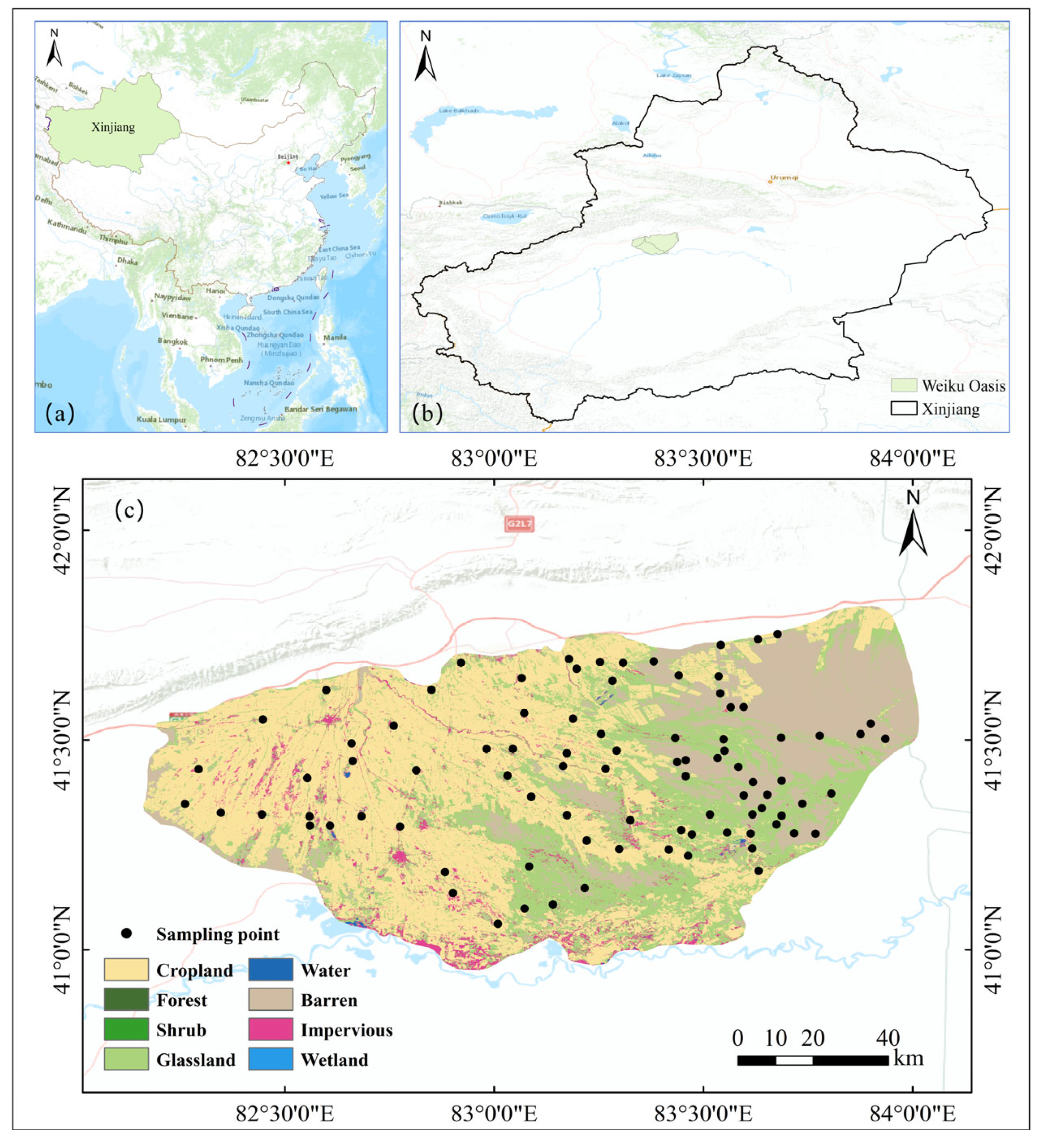
2.1. Study Area

The Weiku Oasis is situated in the arid region of northwest China, at the northern boundary of the Taklamakan Desert and the southern part of the central Tianshan Mountains (Figure 1). The geographical coordinates span from 82°8′20″E to 83°39′50″E and from 40°59′13″N to 41°54′35″N. The terrain descends from the northwest to the southeast, with elevations ranging between 900 and 2000 m. This region experiences a continental warm temperate arid climate, characterized by a multi-year average temperature of 11.6 °C, an average annual precipitation of 52 mm, and an evaporation-to-precipitation ratio of 54:1 [28]. The Weiku Oasis features diverse soil types, predominantly alluvial soils and meadow soils, with extensive areas of marsh soils, saline soils, and brown calcium soils. The natural vegetation primarily includes Tamarix ramosissima, Populus euphratica, and Herculaneum strobilaceum [29]. Situated within China’s arid regions, the Weiku Oasis represents a relatively typical and complete piedmont alluvial fan plain oasis. Primarily located in Kuqa City, Xayar County, and Shaya County of the Aksu Prefecture in Xinjiang, the oasis covers an area of 5609.6 km2, accounting for 10.7% of the total area of these counties [30]. As a typical irrigated oasis in Xinjiang, it serves as a core area for economic development in southern Xinjiang. Intensive irrigation agriculture has accelerated the diffusion of deep soil salts and the accumulation of surface soil salts [31]. There is an urgent need to assess and manage the soil salinization in the Weiku Oasis to ensure the health and sustainable development of the oasis ecosystem.

2.2. Datasets

The satellite data employed in this study comprise synthetic aperture radar (SAR) and microwave remote sensing data from the European Space Agency’s Sentinel-1, alongside optical multispectral remote sensing data from Sentinel-2. Both data sets, sourced from the Copernicus Data Space Ecosystem (https://dataspace.copernicus.eu/, (accessed on 14 May 2024)), correspond to 19 June 2022 and 15 June 2022, respectively, ensuring temporal alignment with the field sampling data. The DEM data were derived from the ASTER-GDEM V3 dataset, available for download from NASA Earthdata (https://www.earthdata.nasa.gov/, (accessed on 14 May 2024)), and primarily include elevation, slope, and aspect data for the study area. Field data were collected through soil sampling in the field, followed by laboratory measurements of soil electrical conductivity and soil salt content (SSC). Table 1 details the key parameters of each dataset, providing fundamental data for further analysis.

2.2.1. Remote Sensing Data

The Sentinel-1 satellite, a component of the European Space Agency’s Copernicus Programme (GMES), comprises two satellites, Sentinel-1A and Sentinel-1B, equipped with C-band synthetic aperture radar. With a six-day revisit period, it provides continuous, all-weather, day-and-night imagery, making it highly suitable for applications in marine monitoring, land monitoring, and emergency services [32,33]. The IW mode of Sentinel-1 employs a dual polarization combination of VV and VH [34]. This dual polarization mode is particularly suitable for land cover classification, natural disaster assessment, and crop monitoring. This study selected Sentinel-1 SAR GRD image data in IW mode.
Sentinel-2—comprising two satellites, Sentinel-2A and Sentinel-2B—is equipped with high-performance multispectral imaging instruments covering 13 spectral bands, ranging from visible light to near-infrared. These satellites are specifically designed for monitoring the Earth’s land surface, with spatial resolutions ranging from 10 to 30 m, enabling the capture of subtle surface changes [35,36]. This study used the COPERNICUS/S2_SR_HARMONIZED dataset on the Google Earth Engine cloud computing platform for multispectral index calculation. This dataset leverages the 13 spectral bands of Sentinel-2A and Sentinel-2B satellites, covering visible to near-infrared light, providing surface reflectance data after atmospheric correction. The main bands have a spatial resolution of 10 m, suitable for detailed surface monitoring [37].
ASTER GDEM V3 provides high-precision elevation information for the global land surface from 83 degrees north to 83 degrees south latitude [38]. This dataset is available in GeoTIFF format at 1-arc-second (approximately 30 m) spatial resolution, widely accessible for free download through NASA’s Earth data system. ASTER GDEM V3 features improved algorithms enhancing data quality, with median elevation errors within approximately 20 m, significantly better than earlier versions. Its precise elevation information is valuable for watershed analysis, ecosystem research, and natural disaster risk assessment [39].

2.2.2. Measured SSC

To avoid irrigation and rainfall during soil sampling and ensure synchronization with satellite overpass times, field sampling was conducted from 10 June to 30 June 2022. Considering factors such as vegetation cover and soil characteristics, 89 representative sampling points were identified for soil collection. These sampling points were spaced over 1 km apart, uniformly distributed across cultivated areas, transitional desert areas, and outside the oasis to ensure comprehensive spatial coverage. In the predetermined sampling areas, soil samples were collected from the surface (0–10 cm) using the five-point sampling method, with each sampling point’s coordinates recorded using a handheld GPS device. After collecting the soil samples, they were quickly placed into numbered plastic bags for preservation and then transported to the laboratory for processing. The laboratory soil sample processing mainly included the following steps: (1) All samples were air-dried in the laboratory. (2) Fully dried soil samples were sieved to remove impurities and ground into powder, passed through a 0.5 mm sieve. (3) The powdered soil samples were placed in numbered conical flasks for solution preparation, with a soil-to-water ratio of 1:5. (4) The prepared solution was thoroughly shaken and left to stand for 24 h. (5) The solution was filtered using filter paper, and the upper clear liquid was used for measuring electrical conductivity and SSC.

2.3. Methods

This study utilizes satellite observation data from Sentinel-1 and Sentinel-2, along with Digital Elevation Model (DEM) data, to compile a feature variable dataset, with soil salinity content from field-collected soil samples serving as the target variable. Initially, the final feature variable importance is determined by weighted calculations using three feature variable selection algorithms. Subsequently, three different machine learning algorithms are employed to develop soil salinity inversion models, screening for the optimal results. The optimal model is then used to invert the soil salinization distribution of the Weiku Oasis. The overall technical roadmap of this study is illustrated in Figure 2.

2.3.1. Dataset Division

According to the grading standards for soil salinization in arid, semi-arid, and desert regions, the 89 soil samples were classified into five categories: non-saline soil (salt content < 0.2%), lightly saline soil (0.2–0.3%), moderately saline soil (0.3–0.5%), heavily saline soil (0.5–1.0%), and salted soil (>1.0%). The soil salinity of each category was randomly divided into modeling and validation sets in a 2:1 ratio. The statistical analysis of the soil samples after salinization grading is shown in Table 2.
From Table 2, it is evident that the 89 soil samples collected in June were predominantly non-saline and salted soils, comprising 39% and 48% of the total samples, respectively. The modeling and validation sets, which were randomly divided, exhibit similar upper quartile, lower quartile, and median values, indicating comparable distribution structures (Figure 3). Thus, the soil salinity characteristics of these two datasets can be considered representative of the entire dataset.

2.3.2. Backscatter Coefficient

To ensure the accuracy and usability of Sentinel-1 image information, the processing steps for Sentinel-1 GRD format data include the following: (1) orbit correction to adjust satellite positioning errors, (2) thermal noise removal to enhance signal clarity, (3) radiometric calibration to maintain image brightness and contrast consistency, (4) using the Refined Lee filter to remove speckle noise, (5) terrain correction using the range-Doppler method, and (6) conversion to decibels. These steps were completed in SNAP 10.0.0. The decibel-converted VH and VV polarization images were exported as TIFF files for polarization combination calculations.
The effective radar backscatter coefficient is closely related to the soil’s complex permittivity and is a key parameter for microwave remote sensing of soil properties [40]. Ma [41] indicated that combining different radar polarization modes can improve the correlation between the radar backscatter coefficient and soil salinity, thus achieving better soil salinity prediction. This study used ArcGIS to perform raster calculations to obtain eight indices, including single polarization modes (Table 3).

2.3.3. Multispectral Indices

Vegetation under salt stress exhibits specific spectral responses [42], which can be monitored using vegetation indices. New salinity detection models can be constructed based on the spectral information of vegetation and soil, thereby improving inference accuracy [43]. There is a high correlation between salinity indices and soil electrical conductivity, and various salinity indices can regionally reflect salinity and assess its intensity [44]. Therefore, this study selected 10 vegetation and salinity indices that can effectively invert soil salinity content as feature variables for the inversion model. These 10 indices are Normalized Difference Moisture Index (NDMI), Vegetation Moisture Index (VMI), Non-Linear Vegetation Index (NLVI), Generalized Difference Vegetation Index (GENDVI), Enhanced Vegetation Index (EVI), EVI2, salinity indices S1, S2, and S3, and Canopy Response Salinity Index (CRSI). NDMI and VMI are key indices for assessing vegetation moisture content [45,46]. Since increased soil salinity typically leads to a reduction in vegetation moisture, these two indices can indirectly identify and evaluate salinity stress by monitoring changes in vegetation moisture. NLVI, GENDVI, EVI, and EVI2 reflect soil salinity content indirectly by evaluating vegetation greenness, coverage, and growth vitality [47,48,49,50]. High soil salinity usually inhibits vegetation growth, and the trends in these indices can reveal the impact of salinity on vegetation, thereby inferring soil salinity levels. S1, S2, S3, and CRSI are specifically designed to detect and quantify the salinity content of soil and vegetation canopies [51,52]. S1, S2, and S3 directly reflect changes in soil salinity, while CRSI captures the effects of salinity on the vegetation canopy through canopy reflectance characteristics. The constructed multispectral indices and their corresponding expressions are shown in Table 3. The calculations of the multispectral indices were performed on the GEE cloud platform and exported as GeoTiff files.
Table 3. Feature variables and their formulation/simple description (in Sentinel-2 imagery: ρ B L U E = Band 2, ρ G R E E N = Band 3, ρ R E D = Band 4, ρ N I R = Band 8, ρ S W I R 1 = Band 11).
DatasetFeaturesFormulation/Simple DescriptionReference
Sentinel-1Backscatter coefficient V V ,   V H ,   V V + V H ,   V V × V H , V V V H ,   V H V V ,   V H 2 ,   V V 2   [41]
Sentinel-2NDMI N D M I = ρ N I R ρ S W I R 1 ρ N I R + ρ S W I R 1 [45]
VMI V M I = ( ρ N I R + 0.1 ) ( ρ S W I R 1 + 0.02 ) ( ρ N I R + 0.1 ) + ( ρ S W I R 1 + 0.02 ) [46]
NLVI N L V I = ρ N I R 2 ρ R E D ρ N I R 2 + ρ R E D [47]
GENDVI G E N D V I = ρ N I R 2 ρ R E D 2 ρ N I R 2 + ρ R E D 2 [48]
EVI E V I = 2.5 ( ρ N I R ρ R E D ) ρ N I R + 6 ρ R E D 7.5 ρ B L U E + 1 [49]
EVI2 E V I 2 = 2.5 ( ρ N I R ρ R E D ) ρ N I R + 2.4 ρ R E D + 1 [50]
S1 S 1 = ρ B L U E ρ R E D [51]
S2 S 2 = ρ B L U E ρ R E D ρ B L U E + ρ R E D [51]
S3 S 3 = ρ G R E E N × ρ R E D ρ B L U E [51]
CRSI C R S I = ρ N I R × ρ R E D ( ρ G R E E N × ρ B L U E ) ρ N I R × ρ R E D + ( ρ G R E E N × ρ B L U E ) [52]
ASTER-GDEM V3DEMElevation[16]
Slope
Aspect

2.3.4. Topographic Features

Topographic factors significantly influence soil salinization by affecting water flow, deposition, and evaporation processes. Slope influences water flow and deposition processes, thus affecting the distribution of soil salts [53]. Aspect determines the amount of solar radiation and evaporation rate, thereby influencing soil moisture and salt distribution [54]. Elevation affects temperature and precipitation, impacting soil moisture and salt distribution [16]. To avoid unnecessary errors due to different resolutions, the DEM data of the study area from ASTER GDEM V3 was resampled to 10 m resolution in ENVI 5.6. Subsequently, ArcGIS 10.8 was used to extract elevation, slope, and aspect as feature variable data (Table 3).

2.3.5. Feature Variable Importance Evaluation

Evaluating the importance of feature variables helps to understand the prediction mechanism of the model. Feature importance indicates the impact of each predictor variable on the model’s results. These evaluations not only help to interpret the model but also guide variable selection, thereby improving the model’s performance [55]. Defining variable importance as the comparison of predictive ability among all features provides better interpretability and consistency. This approach is applicable to various regression techniques and can construct effective confidence intervals, enhancing model interpretability [56].
Recursive feature elimination (RFE) generates multiple candidate subsets by recursively removing the least important features, ultimately determining the optimal subset [57]. The Random Forest Regressor feature importance method evaluates feature importance by analyzing the split points of each decision tree. First, a random forest model is trained using all features. The random forest consists of multiple decision trees, each trained with a random subset of samples and features. Split nodes within each tree are selected based on a feature, and the contribution of this feature to the target variable is calculated. The contributions from all tree splits are aggregated to obtain the importance score for each feature [58]. PLS Regression simplifies the data structure by projecting input data into a new low-dimensional space, then performing regression analysis. Variable Importance in Projection (VIP) scores are used to evaluate the significance of each feature within the PLS model [59].
To accurately evaluate the importance of feature variables used in this study, the evaluation scheme for feature variable importance is performed as follows: StandardScaler is used to standardize the features, making their mean 0 and variance 1. RFE, Random Forest Regressor feature importance, and VIP scores from PLS Regression are selected to calculate the importance of feature variables. MinMaxScaler is used to normalize the RFE scores, random forest importance scores, and VIP scores, ensuring all scores range from 0 to 1. The comprehensive importance score of the three methods is calculated, and the weighted average of the three scores is used as the final variable importance result, which is then sorted.

2.3.6. Machine Learning Models

This study compares the AdaBoost, LightGBM, and CatBoost machine learning methods to select the optimal inversion model for analyzing soil salinization in the Weiku Oasis.
AdaBoost constructs a strong classifier by combining multiple weak classifiers. Its core principle is to adjust the sample weights based on the error rate of the previous round in each training round, giving more attention to misclassified samples in the next round, thereby gradually improving the overall performance of the model. This adaptive adjustment effectively enhances prediction accuracy, especially when dealing with noisy data. Its main advantages include significantly improving the performance of weak classifiers, strong adaptability, and simple algorithm implementation, making it widely applicable to various classification problems [60]. The AdaBoost model parameters used in this study include “max_depth”, “min_samples_split”, “min_samples_leaf”, “min_weight_fraction_leaf”, and “max_features”. These parameters control the depth of the decision trees, splitting conditions, minimum samples per leaf node, minimum sample weight, and the proportion of features used at each split, respectively. The parameters “n_estimators” and “learning_rate” control the number of base learners and the step size for weight updates during each iteration. Additionally, the loss function type is set to “linear”. These parameters collectively adjust the model’s complexity and learning rate, and help prevent overfitting.
LightGBM is an algorithm that accelerates the growth process of decision trees through histogram-based discretization and bucketing of feature values. This gives LightGBM significant advantages in training speed and memory efficiency. It supports distributed training and is well-suited for handling large-scale datasets. LightGBM has shown excellent performance in various machine learning competitions, demonstrating its high accuracy and robustness. Its main advantages are efficient training, the ability to handle large-scale data, and high prediction accuracy in various application scenarios [61]. The LightGBM model trained in this study uses the “dart” boosting type, with key parameters including “num_leaves”, “learning_rate”, “max_depth”, and “n_estimators”, which control the complexity of the trees, learning rate, maximum depth, and number of iterations. To prevent overfitting, parameters such as “min_child_samples”, “colsample_bytree”, “reg_alpha”, “reg_lambda”, “bagging_fraction”, and “feature_fraction” are used. These parameters improve the model’s robustness and generalization ability by controlling the minimum number of samples per leaf, the proportion of features used per tree, and the regularization strength.
CatBoost is a GBDT algorithm optimized for handling categorical features. It adopts the ordered boosting method, gradually introducing target encoding and noise processing to reduce overfitting and training bias. CatBoost automatically handles missing values and categorical features, simplifying the data preprocessing process and significantly improving the model’s generalization ability and stability. Its main advantages are optimized handling of categorical features, automated data processing, and high stability and performance on various datasets. CatBoost has shown outstanding performance in practical applications when dealing with complex data [62]. The CatBoost model parameters used in this study include “iterations”, “learning_rate”, and “depth”. These parameters directly impact the model’s performance and complexity. “Iterations” determines the number of trees trained, “learning_rate” controls the step size for weight updates during each iteration, and “depth” determines the complexity of the decision trees. To prevent overfitting, parameters such as “L2_leaf_reg”, “bagging_temperature”, “random_strength”, “rsm”, and “subsample” are used. These parameters enhance the model’s robustness by adding regularization constraints, increasing the diversity of training data, and controlling the proportion of features and data samples used per tree.
To obtain the optimal parameter settings for the three models, a large parameter search space is first defined. Bayesian optimization is then used to search within this space, evaluating the model’s performance with different parameter combinations through 4-fold cross-validation. The best-performing combinations are identified and then manually fine-tuned to determine the final parameters used to train the models.

2.3.7. Model Accuracy Evaluation

To evaluate the performance of soil salinity prediction models, this study uses the coefficient of determination (R2), root mean square error (RMSE), and mean absolute error (MAE) as evaluation metrics. The calculation formulas for the evaluation metrics are as follows:
R 2 = 1 i = 1 n   y i ^ y ¯ 2 i = 1 n   y i y ¯ 2
R M S E = i = 1 n   y i ^ y i 2 n
M A E = 1 n i = 1 n y ^ i y i
where y ^ is the predicted SSC, y ¯ is the mean of the measured sample SSC, y i is the measured sample SSC, and n is the number of samples.
R2 compares the predicted values to the scenario where only the mean is used; a result closer to 1 indicates higher model accuracy. RMSE reflects the actual error of the predicted values, with smaller values indicating higher accuracy. MAE measures the model’s predictive performance by calculating the average absolute error between the observed and predicted values; a lower MAE signifies a smaller difference between predicted and observed values, indicating better model performance.

3. Results and Analysis

3.1. Variable Correlation Analysis

A Pearson correlation analysis was conducted between the radar backscatter coefficients and their polarization combination indices, 10 indices calculated from Sentinel-2, and 3 topographic variables with SSC. The results are shown in Figure 4.
From Figure 4, it can be observed that there is generally a strong correlation between radar polarization combinations and vegetation indices (such as EVI, NDMI). This might be because the growth status of vegetation affects the physical properties of the surface, which in turn affects the reflection of radar signals. Almost all vegetation indices usually show a negative correlation with the salinity index S3, indicating that lower vegetation indices may be associated with higher salinity, reflecting the inhibitory effect of salinity on plant growth. There is a high positive correlation between EVI and EVI2, as well as between NDMI and other vegetation indices, suggesting that these indices reflect similar surface characteristics. Overall, there is a significant correlation between all vegetation indices and some radar polarization combinations and topographic factors. Variable selection methods can eliminate unnecessary variable information, reducing model overfitting or underfitting, thus improving model accuracy and robustness. Therefore, further screening and ranking of variables is needed.

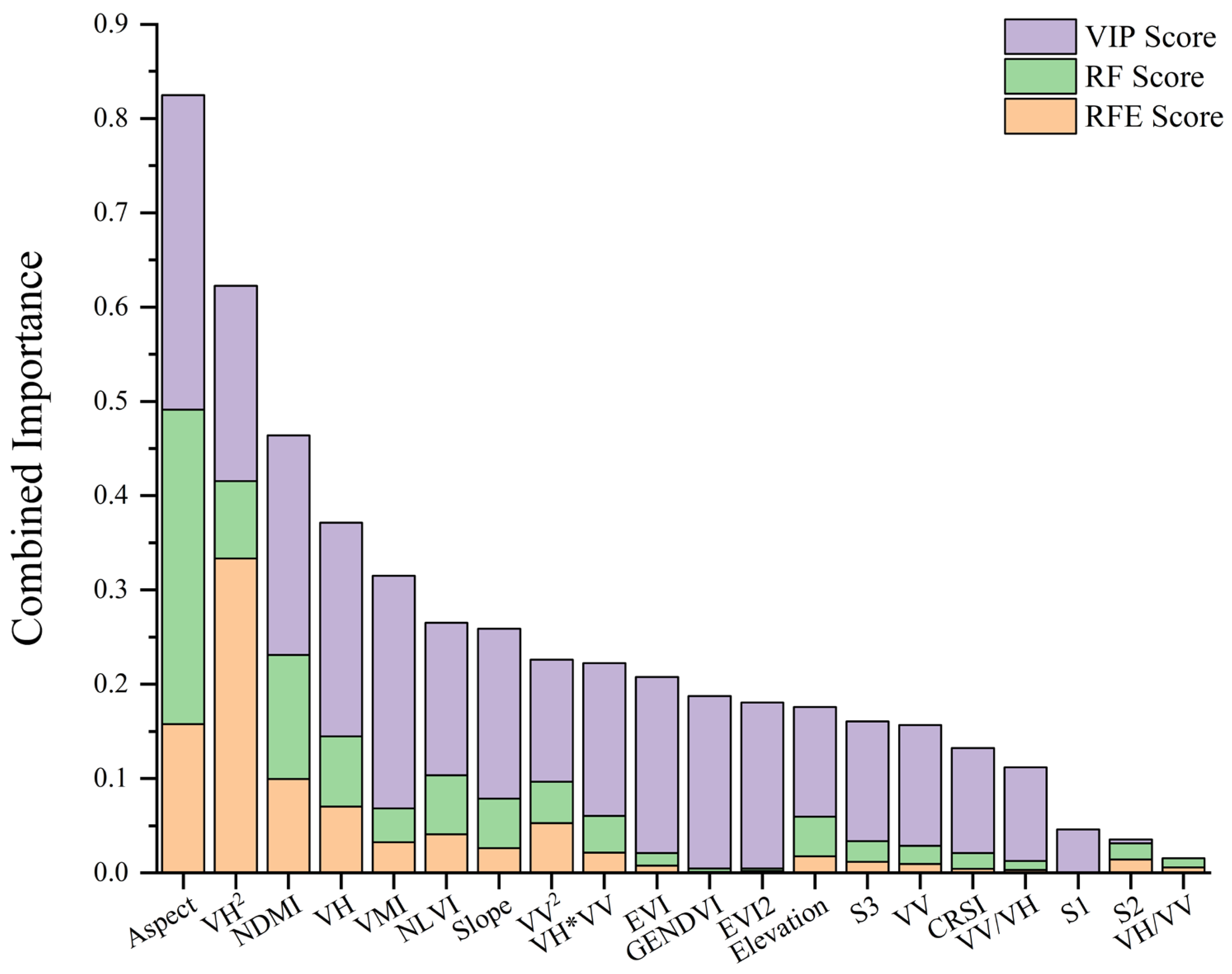
3.2. Feature Variable Importance Ranking

RFE, RF, and VIP methods were used to score the importance of 21 feature variables (2 backscatter coefficients, 6 SAR polarization combination indices, 10 multispectral indices, and 3 topographic factors) and normalize them for subsequent weighted calculations. The results of the three models’ scores are shown in Figure 5.
In the RFE scoring, Aspect is shown as the most important feature. This might indicate that topographic orientation plays a key role in determining surface characteristics (such as soil type and vegetation status), which are crucial for the predictive model (soil salinity content). VH2 and NDMI also showed high importance, suggesting that these variables (radar polarization data and vegetation indices) have strong explanatory power in the model. VV, CRSI, and S1 scored lower, indicating that these features contribute less to the model in the RFE method.
Similar to RFE, Aspect also showed the highest importance in the RF importance scoring model. This further confirms the critical role of topographic orientation in influencing model predictions. Unlike RFE, VH and VV importance increased in the RF importance scoring model, which might be because random forest handles complex interactions between variables better, making more effective use of these radar data. CRSI and S1 still maintained low importance, suggesting that these variables might contribute little to the predictive target in multiple models.
In the VIP method, Aspect and VV/VH scored significantly higher, indicating strong explanatory power in the model. Particularly, the Aspect factor showed extremely high importance in all three evaluation methods. EVI and GENDVI also showed high importance, related to their ability to reflect vegetation health and related ecological parameters. Similar to the previous methods, CRSI and S1 performed poorly in the VIP method, further indicating their low variability related to the main predictive target in the dataset.
Given the differences in results from different scoring methods, a weighted scoring method was proposed to obtain better feature variable scoring results. Four-fold cross-validation was used to evaluate each method. Based on the RMSE of the cross-validation results, weights were determined for each feature selection method. The final importance score for each feature was calculated by weighting according to each method’s weight, and the final feature importance scores were ranked and output. The final scoring results are shown in Figure 6. The top five feature variables include topography, visible light indices, and radar polarization indices, with Aspect having the highest comprehensive score.

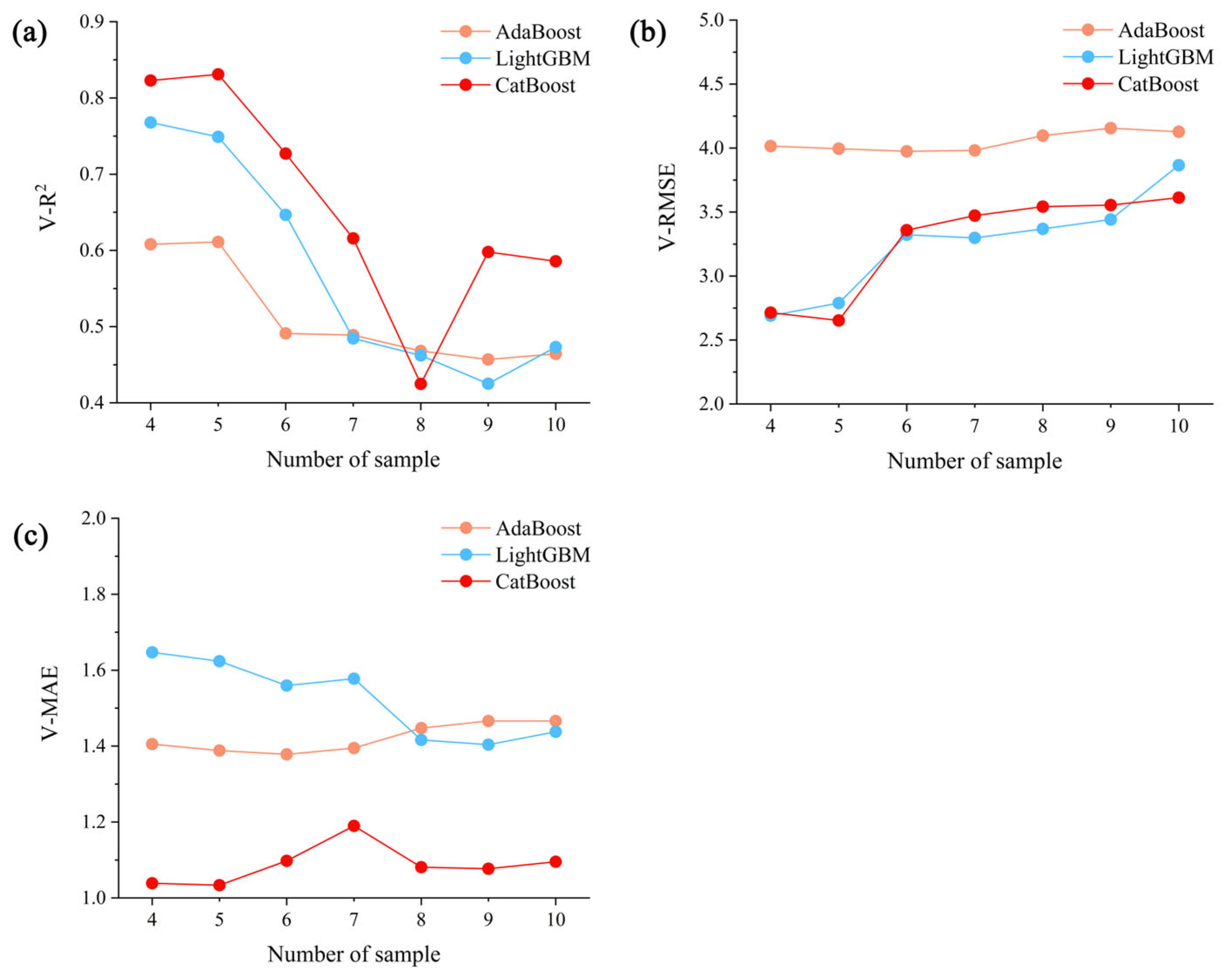
3.3. Comparison of Model Accuracy

To validate the effectiveness of the normalized weighted importance scoring scheme, determine the optimal number of feature variables, and find the optimal SSC inversion model, this study selected the top 10 feature variables ranked by importance in Figure 6. The number of feature variables was sequentially chosen as the top 4, top 5, top 6, and so on, up to the top 10. According to the division method in Table 2, the 89 measured SSC points and their corresponding feature variables were divided into training and validation sets. SSC inversion modeling was conducted using AdaBoost, LightGBM, and CatBoost machine learning models, and model accuracy and stability were evaluated using R2, RMSE, and MAE indicators. The results are shown in Figure 7. V-R2, V-RMSE, and V-MAE represent R2, RMSE, and MAE for the validation set, respectively.
As seen in Figure 7, with the increase in parameters, the R2 of all three models shows a decreasing trend, while RMSE and MAE show an increasing trend, indicating that with more feature parameters, the model’s fitting accuracy decreases and robustness weakens. This trend demonstrates the importance of parameter optimization. Compared to previous studies [23,24], using normalized weighted importance scoring can effectively identify important variables, thereby reducing the number of input feature variables while enhancing the model’s inversion accuracy.
Among the models, LightGBM performed best when selecting the top four parameters as feature variables, with an R2 of 0.768, RMSE of 3.995, and MAE of 1.388. The AdaBoost and CatBoost models both performed best when selecting the top five parameters as feature variables, with AdaBoost having an R2 of 0.611, RMSE of 2.690, and MAE of 1.647, and CatBoost having an R2 of 0.831, RMSE of 2.653, and MAE of 1.034. The overall high RMSE might be due to the large variability in soil salinization in the Weiku region and the high number of salt soil samples, leading to more outliers in the model. Overall, the CatBoost model, using Aspect, VH2, NDMI, VH, and VMI as the input feature variables, achieved the highest inversion accuracy and model stability.
Figure 8 shows scatterplots of measured SSC and predicted SSC for the validation set under optimal feature variable settings for different models. The shaded area represents the 95% confidence interval, the blue solid line is the fitted line, and the gray dashed line is the 1:1 line. From Figure 8c, it can be seen that the scatter points of measured and predicted SSC under the optimal feature variable setting of the CatBoost model are closer to the 1:1 line. Figure 8a,b show that the scatter points of measured and predicted SSC under the optimal feature variable settings of the AdaBoost and LightGBM models are more scattered, with the fitted line deviating from the 1:1 line. Additionally, combining the three models, it is clear that the prediction effect is better for lower SSC values, but the prediction results are not ideal for higher SSC values. The prediction results show an overestimation of low values within the confidence interval.

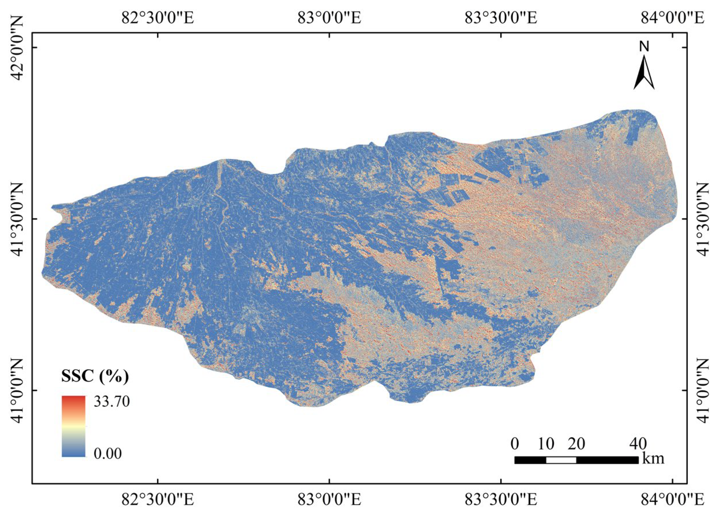
3.4. The SSC Distribution Map of the Study Area Based on the CatBoost Model Inversion

Based on the above results, this study finally used the CatBoost model with Aspect, VH2, NDMI, VH, and VMI as feature variables to invert the surface soil salinity in the study area, obtaining the SSC inversion map of the Weiku Oasis for June 2022 (Figure 9). The SSC is relatively low in the northwestern area of the oasis, while soil salinity gradually increases from the interior to the exterior, with higher SSC observed in the eastern and southwestern desert areas.

4. Discussion

In previous SSC inversion studies, researchers have typically focused on spectral or radar information. Most existing studies model the correlation between soil salinity and spectral characteristics, leveraging the impact of soil salinity on spectral reflectance properties [63,64,65]. However, soil salinization is a complex physicochemical process involving various environmental and human factors. In this study, the topographic factor Aspect scored highest in the comprehensive importance of feature variables, indicating that topographic characteristics significantly influence soil salinization. This finding aligns with other studies that have highlighted the critical role of topographic factors in determining surface characteristics [15]. Soil salinization is also influenced by soil texture and structure, groundwater levels, irrigation and drainage management, and vegetation cover [66]. Future soil salinization monitoring studies should comprehensively consider these factors to develop more accurate and robust monitoring models.
In the correlation analysis of variables in this study, high correlations were observed among radar polarization combinations, vegetation indices, and salinity indices, but these variables showed weak correlations with measured SSC. This may be because the Pearson correlation coefficient measures the strength of linear relationships between two variables, whereas soil salinization is a complex nonlinear process. Nonlinear models typically outperform linear models in soil salinization prediction [67]. CatBoost can capture complex nonlinear relationships between features during modeling, which is crucial for addressing complex environmental issues like soil salinity. When predicting environmental variables, CatBoost captures nonlinear relationships between features better than other boosting algorithms such as LightGBM and AdaBoost, providing higher prediction accuracy [68]. This also explains why the CatBoost model performed best in SSC inversion in this study.
Furthermore, analyzing the results of the validation set for the three models revealed an overestimation of low SSC values, even in the CatBoost model, which had the best performance. This issue relates to the nature of regression algorithms. Many loss functions in machine learning regression models aim to minimize the distance between actual and predicted values, potentially causing the predicted distribution to cluster around the mean of the target variable. The larger errors in high SSC predictions might result from extreme high and low values in the soil salinity data, significantly impacting model training. These extreme values might be treated as outliers by the model, leading to inaccurate predictions for these data. This phenomenon is particularly evident for high salinity levels, where the model may lack sufficient training samples to capture these high salinity patterns accurately [69]. To address these issues, methods such as data smoothing and logarithmic transformation can be used to handle extreme values, making the data distribution more uniform. Additionally, stratified sampling can ensure that the training set includes sufficient high- and low-salinity samples, improving the model’s predictive performance in these areas. In terms of model improvement, ensemble learning methods like RF and ensemble boosting, which combine predictions from multiple models, can reduce bias and variance issues in individual models, enhancing the overall predictive performance [70].

5. Conclusions

This study utilized multi-source remote sensing data, selecting a feature variable dataset composed of 8 radar polarization combinations, 10 spectral indices, and 3 topographic factors. Using a normalized weighted variable selection method, the most important feature variables were identified. Soil salinity inversion models were developed using three machine learning methods—AdaBoost, LightGBM, and CatBoost—and their performance was evaluated. The main conclusions are summarized as follows: There is generally a strong correlation between radar polarization combinations and vegetation indices, and various vegetation indices show a very high correlation with the salinity index S3. The top five feature variables, in order of importance, are Aspect, VH2, NDMI, VH, and VMI. These include topographic variables, spectral indices, and radar polarization indices. The normalized weighted importance scoring method effectively identifies important variables, reducing the number of input features while improving the accuracy of the inversion model. Among the three machine learning models, CatBoost demonstrated the best overall performance in SSC prediction. Combined with the top five feature variables, CatBoost achieved the highest accuracy in the prediction phase (R2 = 0.831, RMSE = 2.653, MAE = 1.034).
This study proposes a novel feature variable selection method and confirms the effectiveness of the CatBoost model in soil salinity inversion. The results provide insights for the further development and application of multi-source remote sensing data in monitoring soil salinization. Future research on soil salinity inversion will consider integrating soil texture, groundwater level, irrigation, and drainage management factors. It will also explore advanced ensemble learning and deep learning algorithms to enhance model performance and accuracy. By constructing an intelligent sensor network, continuous monitoring and data collection of soil salinity can be achieved, providing richer data support for model training. Furthermore, the development of dynamic monitoring methods based on time-series data will enable real-time monitoring and prediction of soil salinization.

Author Contributions

Z.J.: Conceptualization, Methodology, Software, Validation, Formal Analysis, Investigation, Visualization, Writing—Original Draft, and Writing—Review and Editing. Z.H.: Methodology, Validation, Investigation, Writing—Review and Editing, Funding Acquisition, and Project Administration. J.D.: Conceptualization, Supervision, and Funding Acquisition. Z.M.: Investigation. Y.Z.: Investigation. A.A.: Resources. X.J.: Resources. H.C.: Data Curation. W.M.: Supervision. All authors have read and agreed to the published version of the manuscript.

Funding

This research was funded by the Research Project on Spatial and Temporal Evolution of Soil Salinization in the Aksu River Basin (NO. 11N457603776202312202), the Technology Innovation Team (Tianshan Innovation Team), Innovative Team for Efficient Utilization of Water Resources in Arid Regions (NO.2022TSYCTD0001), the Key Project of Natural Science Foundation of Xinjiang Uygur Autonomous Region (No. 2021D01D06), and the National Natural Science Foundation of China (No. 41961059).

Data Availability Statement

The data presented in this study are available upon request from the corresponding author. The data are not publicly available due to confidentiality concerns.

Conflicts of Interest

The authors declare no conflicts of interest.

References

  1. Guo, S.S.; Ruan, B.Q.; Chen, H.R.; Guan, X.Y.; Wang, S.L.; Xu, N.N.; Li, Y.P. Characterizing the spatiotemporal evolution of soil salinization in Hetao Irrigation District (China) using a remote sensing approach. Int. J. Remote Sens. 2018, 39, 6805–6825. [Google Scholar] [CrossRef]
  2. Shahid, S.A.; Zaman, M.; Heng, L. Soil Salinity: Historical Perspectives and a World Overview of the Problem. In Guideline for Salinity Assessment, Mitigation and Adaptation Using Nuclear and Related Techniques; Springer International Publishing: Cham, Switzerland, 2018; pp. 43–53. [Google Scholar] [CrossRef]
  3. Qadir, M.; Quillérou, E.; Nangia, V.; Murtaza, G.; Singh, M.; Thomas, R.J.; Drechsel, P.; Noble, A.D. Economics of salt-induced land degradation and restoration. Nat. Resour. Forum 2014, 38, 282–295. [Google Scholar] [CrossRef]
  4. Seifi, M.; Ahmadi, A.; Neyshabouri, M.-R.; Taghizadeh-Mehrjardi, R.; Bahrami, H.-A. Remote and Vis-NIR spectra sensing potential for soil salinization estimation in the eastern coast of Urmia hyper saline lake, Iran. Remote Sens. Appl. Soc. Environ. 2020, 20, 100398. [Google Scholar] [CrossRef]
  5. Zhu, C.; Ding, J.; Zhang, Z.; Wang, Z. Exploring the potential of UAV hyperspectral image for estimating soil salinity: Effects of optimal band combination algorithm and random forest. Spectrochim. Acta Part A Mol. Biomol. Spectrosc. 2022, 279, 121416. [Google Scholar] [CrossRef] [PubMed]
  6. Wang, J.Z.; Ding, J.L.; Yu, D.L.; Ma, X.K.; Zhang, Z.P.; Ge, X.Y.; Teng, D.X.; Li, X.H.; Liang, J.; Lizag, A.; et al. Capability of Sentinel-2 MSI data for monitoring and mapping of soil salinity in dry and wet seasons in the Ebinur Lake region, Xinjiang, China. Geoderma 2019, 353, 172–187. [Google Scholar] [CrossRef]
  7. Wang, N.; Xue, J.; Peng, J.; Biswas, A.; He, Y.; Shi, Z. Integrating Remote Sensing and Landscape Characteristics to Estimate Soil Salinity Using Machine Learning Methods: A Case Study from Southern Xinjiang, China. Remote Sens. 2020, 12, 4118. [Google Scholar] [CrossRef]
  8. Wang, J.; Peng, J.; Li, H.; Yin, C.; Liu, W.; Wang, T.; Zhang, H. Soil Salinity Mapping Using Machine Learning Algorithms with the Sentinel-2 MSI in Arid Areas, China. Remote Sens. 2021, 13, 305. [Google Scholar] [CrossRef]
  9. Davis, E.; Wang, C.; Dow, K. Comparing Sentinel-2 MSI and Landsat 8 OLI in soil salinity detection: A case study of agricultural lands in coastal North Carolina. Int. J. Remote Sens. 2019, 40, 6134–6153. [Google Scholar] [CrossRef]
  10. Periasamy, S.; Ravi, K.P.; Tansey, K. Identification of saline landscapes from an integrated SVM approach from a novel 3-D classification schema using Sentinel-1 dual-polarized SAR data. Remote Sens. Environ. 2022, 279, 113144. [Google Scholar] [CrossRef]
  11. Ma, G.; Ding, J.; Han, L.; Zhang, Z.; Ran, S. Digital mapping of soil salinization based on Sentinel-1 and Sentinel-2 data combined with machine learning algorithms. Reg. Sustain. 2021, 2, 177–188. [Google Scholar] [CrossRef]
  12. Yin, H.Y.; Chen, C.; He, Y.J.; Jia, J.D.; Chen, Y.W.; Du, R.Q.; Xiang, R.; Zhang, X.; Zhang, Z.T. Synergistic estimation of soil salinity based on Sentinel-1 image texture and Sentinel-2 salinity spectral indices. J. Appl. Remote Sens. 2023, 17, 018502. [Google Scholar] [CrossRef]
  13. Arjasakusuma, S.; Kusuma, S.S.; Vetrita, Y.; Prasasti, I.; Arief, R. Monthly Burned-Area Mapping using Multi-Sensor Integration of Sentinel-1 and Sentinel-2 and machine learning: Case Study of 2019’s fire events in South Sumatra Province, Indonesia. Remote Sens. Appl. Soc. Environ. 2022, 27, 100790. [Google Scholar] [CrossRef]
  14. Fang, Z.; Heigang, X.; Yuan, T.; Fuming, L. Impacts of Regional Topographic Factors on Spatial Distribution of Soil Salinization in Qitai Oasis. Res. Environ. Sci. 2011, 24, 731–739. [Google Scholar] [CrossRef]
  15. Florinsky, I.V. Chapter 8—Influence of Topography on Soil Properties. In Digital Terrain Analysis in Soil Science and Geology; Florinsky, I.V., Ed.; Academic Press: Boston, MA, USA, 2012; pp. 145–149. [Google Scholar] [CrossRef]
  16. Bannari, A.; Al-Ali, Z.M.; Kadhem, G.M. Effects of Topgraphic Attributes and Water-Table Depths on the Soil Salinity Accumulation in Arid Land. In Proceedings of the 2021 IEEE International Geoscience and Remote Sensing Symposium IGARSS, Brussels, Belgium, 11–16 July 2021; pp. 6548–6551. [Google Scholar] [CrossRef]
  17. Wang, F.; Ding, J.; Wei, Y.; Zhou, Q.; Yang, X.; Wang, Q. Sensitivity analysis of soil salinity and vegetation indices to detect soil salinity variation by using Landsat series images:applications in different oases in Xinjiang, China. Acta Ecol. Sin. 2017, 37, 5007–5022. [Google Scholar]
  18. Sirpa-Poma, J.W.; Satgé, F.; Resongles, E.; Pillco-Zolá, R.; Molina-Carpio, J.; Flores Colque, M.G.; Ormachea, M.; Pacheco Mollinedo, P.; Bonnet, M.-P. Towards the Improvement of Soil Salinity Mapping in a Data-Scarce Context Using Sentinel-2 Images in Machine-Learning Models. Sensors 2023, 23, 9328. [Google Scholar] [CrossRef]
  19. Zhao, Z.-D.; Zhao, M.-S.; Lu, H.-L.; Wang, S.-H.; Lu, Y.-Y. Digital Mapping of Soil pH Based on Machine Learning Combined with Feature Selection Methods in East China. Sustainability 2023, 15, 12874. [Google Scholar] [CrossRef]
  20. Shi, X.; Song, J.; Wang, H.; Lv, X.; Tian, T.; Wang, J.; Li, W.; Zhong, M.; Jiang, M. Improving the monitoring of root zone soil salinity under vegetation cover conditions by combining canopy spectral information and crop growth parameters. Front. Plant Sci. 2023, 14, 1171594. [Google Scholar] [CrossRef]
  21. Zhao, W.; Ma, F.; Yu, H.; Li, Z. Inversion Model of Salt Content in Alfalfa-Covered Soil Based on a Combination of UAV Spectral and Texture Information. Agriculture 2023, 13, 1530. [Google Scholar] [CrossRef]
  22. Hou, J.; Rusuli, Y. Estimation of soil salt content in the Bosten Lake watershed, Northwest China based on a support vector machine model and optimal spectral indices. PLoS ONE 2023, 18, e0273738. [Google Scholar] [CrossRef]
  23. Jia, P.; Zhang, J.; He, W.; Hu, Y.; Zeng, R.; Zamanian, K.; Jia, K.; Zhao, X. Combination of Hyperspectral and Machine Learning to Invert Soil Electrical Conductivity. Remote Sens. 2022, 14, 2602. [Google Scholar] [CrossRef]
  24. Mukhamediev, R.I.; Merembayev, T.; Kuchin, Y.; Malakhov, D.; Zaitseva, E.; Levashenko, V.; Popova, Y.; Symagulov, A.; Sagatdinova, G.; Amirgaliyev, Y. Soil Salinity Estimation for South Kazakhstan Based on SAR Sentinel-1 and Landsat-8,9 OLI Data with Machine Learning Models. Remote Sens. 2023, 15, 4269. [Google Scholar] [CrossRef]
  25. Qi, G.; Chang, C.; Yang, W.; Zhao, G. Soil salinity inversion in coastal cotton growing areas: An integration method using satellite-ground spectral fusion and satellite-UAV collaboration. Land Degrad. Dev. 2022, 33, 2289–2302. [Google Scholar] [CrossRef]
  26. Wei, L.; Yuan, Z.; Wang, Z.; Zhao, L.; Zhang, Y.; Lu, X.; Cao, L. Hyperspectral Inversion of Soil Organic Matter Content Based on a Combined Spectral Index Model. Sensors 2020, 20, 2777. [Google Scholar] [CrossRef]
  27. Gao, Y.; Wang, L.; Zhong, G.; Wang, Y.; Yang, J. Potential of Remote Sensing Images for Soil Moisture Retrieving Using Ensemble Learning Methods in Vegetation-Covered Area. IEEE J. Sel. Top. Appl. Earth Obs. Remote Sens. 2023, 16, 8149–8165. [Google Scholar] [CrossRef]
  28. Ding, J.; Yu, D. Monitoring and evaluating spatial variability of soil salinity in dry and wet seasons in the Werigan–Kuqa Oasis, China, using remote sensing and electromagnetic induction instruments. Geoderma 2014, 235–236, 316–322. [Google Scholar] [CrossRef]
  29. Han, L.; Ding, J.; Wang, J.; Zhang, J.; Xie, B.; Hao, J. Monitoring Oasis Cotton Fields Expansion in Arid Zones Using the Google Earth Engine: A Case Study in the Ogan-Kucha River Oasis, Xinjiang, China. Remote Sens. 2022, 14, 225. [Google Scholar] [CrossRef]
  30. Gulibositan, B.; Ding, J.; Li, Y. Land Use/Land Cover Change and Its Environmental Effects in Ugan-Kuqa River Delta Oasis. Acta Agrestia Sin. 2018, 26, 53–61. [Google Scholar] [CrossRef]
  31. Wang, N.; Peng, J.; Xue, J.; Zhang, X.; Huang, J.; Biswas, A.; He, Y.; Shi, Z. A framework for determining the total salt content of soil profiles using time-series Sentinel-2 images and a random forest-temporal convolution network. Geoderma 2022, 409, 115656. [Google Scholar] [CrossRef]
  32. Torres, R.; Snoeij, P.; Geudtner, D.; Bibby, D.; Davidson, M.; Attema, E.; Potin, P.; Rommen, B.; Floury, N.; Brown, M.; et al. GMES Sentinel-1 mission. Remote Sens. Environ. 2012, 120, 9–24. [Google Scholar] [CrossRef]
  33. Mullissa, A.; Vollrath, A.; Odongo-Braun, C.; Slagter, B.; Balling, J.; Gou, Y.; Gorelick, N.; Reiche, J. Sentinel-1 SAR Backscatter Analysis Ready Data Preparation in Google Earth Engine. Remote Sens. 2021, 13, 1954. [Google Scholar] [CrossRef]
  34. Veloso, A.; Mermoz, S.; Bouvet, A.; Le Toan, T.; Planells, M.; Dejoux, J.-F.; Ceschia, E. Understanding the temporal behavior of crops using Sentinel-1 and Sentinel-2-like data for agricultural applications. Remote Sens. Environ. 2017, 199, 415–426. [Google Scholar] [CrossRef]
  35. Drusch, M.; Del Bello, U.; Carlier, S.; Colin, O.; Fernandez, V.; Gascon, F.; Hoersch, B.; Isola, C.; Laberinti, P.; Martimort, P.; et al. Sentinel-2: ESA’s Optical High-Resolution Mission for GMES Operational Services. Remote Sens. Environ. 2012, 120, 25–36. [Google Scholar] [CrossRef]
  36. Segarra, J.; Buchaillot, M.L.; Araus, J.L.; Kefauver, S.C. Remote Sensing for Precision Agriculture: Sentinel-2 Improved Features and Applications. Agronomy 2020, 10, 641. [Google Scholar] [CrossRef]
  37. Radoux, J.; Chomé, G.; Jacques, D.; Waldner, F.; Bellemans, N.; Matton, N.; Lamarche, C.; D’Andrimont, R.; Defourny, P. Sentinel-2’s Potential for Sub-Pixel Landscape Feature Detection. Remote Sens. 2016, 8, 488. [Google Scholar] [CrossRef]
  38. Gesch, D.; Oimoen, M.; Danielson, J.; Meyer, D. Validation of the Aster Global Digital Elevation Model Version 3 over the Conterminous United States. Int. Arch. Photogramm. Remote Sens. Spatial Inf. Sci. 2016, XLI-B4, 143–148. [Google Scholar] [CrossRef]
  39. Altunel, A.O.; Okolie, C.J.; Kurtipek, A. Capturing the Level of Progress in Vertical Accuracy Achieved by ASTER GDEM since the Beginning: Turkish and Nigerian Examples. Geocarto Int. 2022, 37, 12073–12095. [Google Scholar] [CrossRef]
  40. Wang, X.; Liu, Q.; Qu, Z.; Wang, L.; Li, X.; Wang, Y. Inversion and verification of salinity soil moisture using microwave radar. Trans. Chin. Soc. Agric. Eng. 2017, 33, 108–114. [Google Scholar] [CrossRef]
  41. Ma, C. Quantitative retrieval of soil salt content based on Sentinel-1 dual polarization radar image. Trans. Chin. Soc. Agric. Eng. (Trans. CSAE) 2018, 34, 153–158. [Google Scholar] [CrossRef]
  42. Zhang, T.; Zeng, S.; Gao, Y.; Ouyang, Z.; Li, B.; Fang, C.; Zhao, B. Using hyperspectral vegetation indices as a proxy to monitor soil salinity. Ecol. Indic. 2011, 11, 1552–1562. [Google Scholar] [CrossRef]
  43. Hong, G.; Bai, T.; Wang, X.; Li, M.; Liu, C.; Cong, L.; Qu, X.; Li, X. Extraction and Analysis of Soil Salinization Information in an Alar Reclamation Area Based on Spectral Index Modeling. Appl. Sci. 2023, 13, 3440. [Google Scholar] [CrossRef]
  44. Asfaw, E.; Suryabhagavan, K.V.; Argaw, M. Soil salinity modeling and mapping using remote sensing and GIS: The case of Wonji sugar cane irrigation farm, Ethiopia. J. Saudi Soc. Agric. Sci. 2018, 17, 250–258. [Google Scholar] [CrossRef]
  45. Rokni, K.; Ahmad, A.; Selamat, A.; Hazini, S. Water Feature Extraction and Change Detection Using Multitemporal Landsat Imagery. Remote Sens. 2014, 6, 4173–4189. [Google Scholar] [CrossRef]
  46. Ceccato, P.; Flasse, S.; Grégoire, J.-M. Designing a spectral index to estimate vegetation water content from remote sensing data: Part 2. Validation and applications. Remote Sens. Environ. 2002, 82, 198–207. [Google Scholar] [CrossRef]
  47. Feng, W.; Wu, Y.; He, L.; Ren, X.; Wang, Y.; Hou, G.; Wang, Y.; Liu, W.; Guo, T. An optimized non-linear vegetation index for estimating leaf area index in winter wheat. Precis. Agric. 2019, 20, 1157–1176. [Google Scholar] [CrossRef]
  48. Wu, W. The Generalized Difference Vegetation Index (GDVI) for Dryland Characterization. Remote Sens. 2014, 6, 1211–1233. [Google Scholar] [CrossRef]
  49. Huete, A.; Didan, K.; Miura, T.; Rodriguez, E.P.; Gao, X.; Ferreira, L.G. Overview of the radiometric and biophysical performance of the MODIS vegetation indices. Remote Sens. Environ. 2002, 83, 195–213. [Google Scholar] [CrossRef]
  50. Jiang, Z.; Huete, A.R.; Didan, K.; Miura, T. Development of a two-band enhanced vegetation index without a blue band. Remote Sens. Environ. 2008, 112, 3833–3845. [Google Scholar] [CrossRef]
  51. Abbas, A.; Khan, S. Using remote sensing techniques for appraisal of irrigated soil salinity. In Proceedings of the International Congress on Modelling and Simulation (MODSIM), Christchurch, New Zealand, 10–13 December 2007; pp. 2632–2638. [Google Scholar]
  52. Whitney, K.; Scudiero, E.; El-Askary, H.M.; Skaggs, T.H.; Allali, M.; Corwin, D.L. Validating the use of MODIS time series for salinity assessment over agricultural soils in California, USA. Ecol. Indic. 2018, 93, 889–898. [Google Scholar] [CrossRef]
  53. Morbidelli, R.; Saltalippi, C.; Flammini, A.; Govindaraju, R.S. Role of slope on infiltration: A review. J. Hydrol. 2018, 557, 878–886. [Google Scholar] [CrossRef]
  54. Pelletier, J.D.; Barron-Gafford, G.A.; Gutiérrez-Jurado, H.; Hinckley, E.-L.S.; Istanbulluoglu, E.; McGuire, L.A.; Niu, G.-Y.; Poulos, M.J.; Rasmussen, C.; Richardson, P.; et al. Which way do you lean? Using slope aspect variations to understand Critical Zone processes and feedbacks. Earth Surf. Process. Landf. 2018, 43, 1133–1154. [Google Scholar] [CrossRef]
  55. Chen, J.M. Interpreting Linear Beta Coefficients Alongside Feature Importances in Machine Learning. Atl. Econ. J. 2021, 49, 245–247. [Google Scholar] [CrossRef]
  56. Williamson, B.D.; Gilbert, P.B.; Carone, M.; Simon, N. Nonparametric Variable Importance Assessment Using Machine Learning Techniques. Biometrics 2021, 77, 9–22. [Google Scholar] [CrossRef] [PubMed]
  57. Su, R.; Liu, X.; Wei, L. MinE-RFE: Determine the optimal subset from RFE by minimizing the subset-accuracy–defined energy. Brief. Bioinform. 2019, 21, 687–698. [Google Scholar] [CrossRef] [PubMed]
  58. Voges, L.F.; Jarren, L.C.; Seifert, S. Exploitation of surrogate variables in random forests for unbiased analysis of mutual impact and importance of features. Bioinformatics 2023, 39, btad471. [Google Scholar] [CrossRef]
  59. Zhao, N.; Wu, Z.; Wu, C.; Wang, S.; Zhan, X. Performance evaluation of variable selection methods coupled with partial least squares regression to determine the target component in solid samples. J. Near Infrared Spectrosc. 2022, 30, 171–178. [Google Scholar] [CrossRef]
  60. Cao, Y.; Miao, Q.-G.; Liu, J.-C.; Gao, L. Advance and Prospects of AdaBoost Algorithm. Acta Autom. Sin. 2013, 39, 745–758. [Google Scholar] [CrossRef]
  61. Ke, G.; Meng, Q.; Finley, T.; Wang, T.; Chen, W.; Ma, W.; Ye, Q.; Liu, T.-Y. LightGBM: A highly efficient gradient boosting decision tree. In Proceedings of the 31st International Conference on Neural Information Processing Systems, Long Beach, CA, USA, 4–9 December 2017; pp. 3149–3157. [Google Scholar]
  62. Kang, Y.; Jang, E.; Im, J.; Kwon, C.; Kim, S. Developing a New Hourly Forest Fire Risk Index Based on Catboost in South Korea. Appl. Sci. 2020, 10, 8213. [Google Scholar] [CrossRef]
  63. Ge, X.Y.; Ding, J.L.; Teng, D.X.; Wang, J.Z.; Huo, T.C.; Jin, X.Y.; Wang, J.J.; He, B.Z.; Han, L.J. Updated soil salinity with fine spatial resolution and high accuracy: The synergy of Sentinel-2 MSI, environmental covariates and hybrid machine learning approaches. Catena 2022, 212, 106054. [Google Scholar] [CrossRef]
  64. Taghadosi, M.M.; Hasanlou, M.; Eftekhari, K. Soil salinity mapping using dual-polarized SAR Sentinel-1 imagery. Int. J. Remote Sens. 2019, 40, 237–252. [Google Scholar] [CrossRef]
  65. Fan, X.; Weng, Y.; Tao, J. Towards decadal soil salinity mapping using Landsat time series data. Int. J. Appl. Earth Obs. Geoinf. 2016, 52, 32–41. [Google Scholar] [CrossRef]
  66. Nosetto, M.D.; Acosta, A.M.; Jayawickreme, D.H.; Ballesteros, S.I.; Jackson, R.B.; Jobbágy, E.G. Land-use and topography shape soil and groundwater salinity in central Argentina. Agric. Water Manag. 2013, 129, 120–129. [Google Scholar] [CrossRef]
  67. Boudibi, S.; Sakaa, B.; Benguega, Z.; Fadlaoui, H.; Othman, T.; Bouzidi, N. Spatial prediction and modeling of soil salinity using simple cokriging, artificial neural networks, and support vector machines in El Outaya plain, Biskra, southeastern Algeria. Acta Geochim. 2021, 40, 390–408. [Google Scholar] [CrossRef]
  68. Saber, M.; Boulmaiz, T.; Guermoui, M.; Abdrabo, K.I.; Kantoush, S.A.; Sumi, T.; Boutaghane, H.; Nohara, D.; Mabrouk, E. Examining LightGBM and CatBoost models for wadi flash flood susceptibility prediction. Geocarto Int. 2022, 37, 7462–7487. [Google Scholar] [CrossRef]
  69. Zhong, W.; Zhang, D.; Sun, Y.; Wang, Q. A CatBoost-Based Model for the Intensity Detection of Tropical Cyclones over the Western North Pacific Based on Satellite Cloud Images. Remote Sens. 2023, 15, 3510. [Google Scholar] [CrossRef]
  70. Hancock, J.; Khoshgoftaar, T.M. Performance of CatBoost and XGBoost in Medicare Fraud Detection. In Proceedings of the 2020 19th IEEE International Conference on Machine Learning and Applications (ICMLA), Virtual, 14–17 December 2020; pp. 572–579. [Google Scholar] [CrossRef]
Figure 1. (a) The location of Xinjiang in China. (b) The location of the Weiku Oasis in Xinjiang. (c) Land use types and distribution of sampling points in the research area.
Remotesensing 16 03145 g001
Figure 2. Methodology flow diagram.
Remotesensing 16 03145 g002
Figure 3. Descriptive statistics of soil sample salinity content.
Remotesensing 16 03145 g003
Figure 4. Correlation analysis between variables.
Remotesensing 16 03145 g004
Figure 5. Results of importance scoring of feature variables. (a) RFE Score. (b) RF Score. (c) VIP Score.
Remotesensing 16 03145 g005
Figure 6. Weighted importance score ranking of characteristic variables.
Remotesensing 16 03145 g006
Figure 7. Comparison of evaluation metrics for inverse models. (a) Validation set R2. (b) Validation set RMSE. (c) Validation set MAE.
Remotesensing 16 03145 g007
Figure 8. Scatterplots of measured SSC and predicted SSC for different model validation sets.
Remotesensing 16 03145 g008
Figure 9. SSC inversion results for the Weiku Oasis in June 2022 using the CatBoost model.
Remotesensing 16 03145 g009
Table 1. Datasets used.
DataTypeSpatial ResolutionDate of AcquisitionPolarization Channels/
Spectral Bands
Sentinel-1SAR/microwave10 m19 June 2022VV and VH polarization
Sentinel-2Optical/multi-spectral10 m19 June 202213 multispectral bands
ASTER-GDEM V3Data products30 m, resampled to 10 m2022-
Field dataSoil salt content-10 June 2022–30 June 2022-
Table 2. Descriptive statistics of soil salinity.
Data SetsNumber of Non-Saline Soil SamplesNumber of Lightly Saline Soil SamplesNumber of Moderately Saline Soil SamplesNumber of Heavily Saline Soil SamplesNumber of
Salted Soil Samples
Total set
(n = 89)
3453344
Training set
(n = 59)
2242229
Validation set
(n = 30)
1211115
Disclaimer/Publisher’s Note: The statements, opinions and data contained in all publications are solely those of the individual author(s) and contributor(s) and not of MDPI and/or the editor(s). MDPI and/or the editor(s) disclaim responsibility for any injury to people or property resulting from any ideas, methods, instructions or products referred to in the content.

