Abstract
Accurately classifying the intra-pulse modulations of radar emitter signals is important for radar systems and can provide necessary information for relevant military command strategy and decision making. As strong additional white Gaussian noise (AWGN) leads to a lower signal-to-noise ratio (SNR) of received signals, which results in a poor classification accuracy on the classification models based on deep neural networks (DNNs), in this paper, we propose an effective denoising method based on a denoising diffusion probabilistic model (DDPM) for increasing the quality of signals. Trained with denoised signals, classification models can classify samples denoised by our method with better accuracy. The experiments based on three DNN classification models using different modal input, with undenoised data, data denoised by the convolutional denoising auto-encoder (CDAE), and our method’s denoised data, are conducted with three different conditions. The extensive experimental results indicate that our proposed method could denoise samples with lower values of the SNR, and that it is more effective for increasing the accuracy of DNN classification models for radar emitter signal intra-pulse modulations, where the average accuracy is increased from around 3 to 22 percentage points based on three different conditions.
1. Introduction
Radar emitter signal intra-pulse modulation classification is essential for electronic support measure (ESM) systems, electronic intelligence (ELINT) systems, and radar warning receivers (RWRs) [1,2,3]. Accurately classifying the intra-pulse modulations of radar emitter signals will help estimate the function of the radar, indicate the potential threat, and provide the necessary information for relevant military command strategy and decision making. The increasing number of radar emitters has made the electromagnetic environment more complex in the real environment [4], and radar emitter signals received by receivers are often disturbed by the noise, where the signals are always in a low signal-to-noise (SNR) condition. The SNR is the main factor to consider for a system to classify radar emitter signal intra-pulse modulations, where a low SNR condition will decrease the accuracy of modulations. Therefore, it is important to develop a method to classify radar emitter signal intra-pulse modulations, especially in conditions of lower SNR.
In recent years, deep learning [5,6] has achieved rapid development, and some methods based on deep neural networks (DNNs) have shown great success in intra-pulse modulation classification. The main proposed deep-learning-based methods can be divided into three parts: time-domain-based methods, frequency-domain-based methods, and time–frequency-domain-based methods. In [7], Wu et al. proposed a one-dimensional (1-D) convolution neural network (CNN) with an attention mechanism block to classify seven different intra-pulse modulations, which uses the normalized sequences in the time domain to train the model. In [8], Zhang et al. proposed a 1-D deep residual shrinkage network (DRSN) to recognize the intra-pulse modulation of radar emitter signals, where the DRSN learns the features from time-domain signal sequences directly without any professional knowledge. In [9], Yuan et al. proposed 1-D selective kernel convolutional neural network for the classification of 11 intra-pulse modulations, where the authors first transfer the original time-domain sequences to frequency-domain sequences by discrete Fourier transformation, and then the designed DNN model is trained by the normalized frequency-domain sequences. Similarly, in [10], Yuan et al. proposed a method for classifying the intra-pulse modulations in semi-supervised conditions, where the DNN model used in the framework is also trained by frequency-domain sequences. Except for these 1-D based DNN models, which use 1-D sequences in the time domain or frequency domain, many researchers focus on the time–frequency domain. In [11], the authors first processed the sampled time-domain sequence with a Cohen class time–frequency distribution, and the corresponding results, named time–frequency images (TFIs), were used for training the proposed CNN model. In [12], authors trained the EfficientNet-B0 [13] model by TFIs, where the TFIs used were obtained by converting time-domain radar signals with smooth pseudo-Wigner–Ville distribution transformation (SPWVD). Similarly, in [14,15], for obtaining the TFIs, the authors all chose short-time Fourier transformation (STFT) as the time–frequency analysis tool, and, based on the their own situations, they then proposed the suitable DNN models for classifying the intra-pulse modulations of radar emitter signals.
The existing DNN-based methods have proven their effectiveness for classifying radar emitter signal intra-pulse modulations in good SNR conditions. However, these methods cannot deal with signals in poor SNR conditions, as well as those in good SNR conditions. In environments with a poorer SNR, the signals face serious interference. In order to overcome this problem, some researchers tend to remove noise with different methods. For example, in [16], authors used binarization processing for the TFIs, then a bicubic interpolation; an opening operation and a topological approach are adopted to remove the impacts of noise in TFIs. Similarly, in [11], the authors chose to use 2-D Wiener filtering to remove the influence of noise in TFIs. However, there are still problems in these methods in that they are all based on professional prior knowledge. DNN-based denoising models have been widely used in image processing [17,18,19,20,21] and the related researchers tend to apply them to intra-pulse modulation classification. The most representative work is the convolutional denoising auto-encoder (CDAE) [22]. The CDAE reduces some of the impact of noise on intra-pulse modulation classification and improves the classification accuracy when signals have a lower SNR.
Nonetheless, the denoising method for intra-pulse modulation classification still has considerable room for improvement. Recently, the denoising diffusion probabilistic model (DDPM) [23] has been widely used for image generation. Inspired by the forward process and the reverse process in the DDPM, and by the fact that the noise used in the DDPM is additional white Gaussian noise (AWGN), which is the same as the noise in radar emitter signals [24], in this paper, we proposed an effective denoising method for radar emitter signal intra-pulse modulation classification. The method first selects the sampled time-domain signals higher in SNR. By adding the selected signals with a different power of AWGN with the information of the corresponding time step, the DNN model is trained to predict the added AWGN in the corresponding time step. When the training session is finished, the unselected signals will be sent to the well-trained DNN model with the time step related to the SNR of the signals. Through the reverse process, the signals lower in SNRs could be denoised, and, therefore, the dataset used for training intra-pulse modulation classification will be in a better SNR condition. Several experiments based on the original undenoised dataset, the denoised dataset with the CDAE, and the denoised dataset with our method are conducted. The results show that our denoising method is effective and can significantly improve radar emitter signal intra-pulse modulation classification accuracy, especially in a lower SNR condition.
The main contribution of this paper is that we proposed an effective denoising method for radar emitter signal intra-pulse modulation classification. The dataset denoised by our method could help the classification models, including the time-domain-based DNN model, frequency-domain-based DNN model, and time–frequency-domain-based DNN model, improve their accuracy further compared with the dataset denoised by the most representative CDAE denoising method.
This paper is organized as follows: In Section 2, the proposed method is described in detail. Section 3 shows the dataset used in this paper and the experimental settings. Section 4 describes the extensive experiments and corresponding analysis. Section 5 is the ablation study. Finally, Section 6 draws the conclusion.
2. Materials and Methods
In this paper, we propose an effective denoising method based on DDPM for radar emitter signal intra-pulse modulation classification. In this section, the denoising method based on DDPM will be illustrated in detail. The structure of the denoising model will also be introduced. And the essential parts including SNR estimation and data preprocessing will also be described in detail.
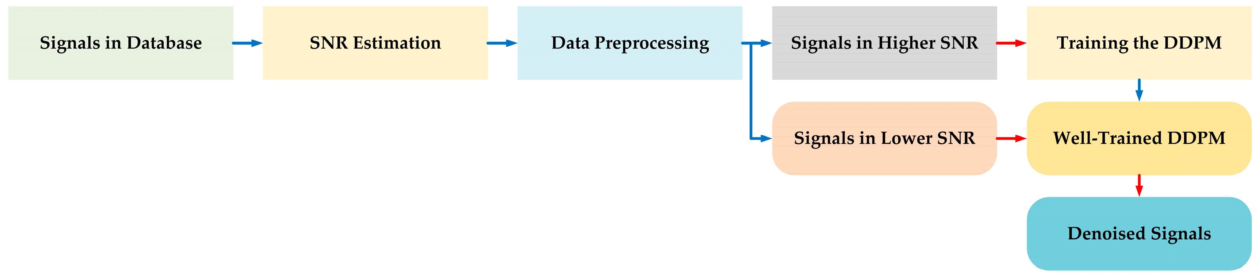
The overall structure of our approach is shown in Figure 1.

Figure 1.
The overall structure of our approach.
In the first part (blue line), the signals in database are first divided into two groups through the processing of SNR estimation and data preprocessing. Then, the group with signals higher in SNR is used for training the DDPM model. After the DDPM is well-trained, the second part (red line) is launched. The group with signals lower in SNR is sent to the well-trained DDPM model, so that the resulting output comprises the relevant denoised signals.
2.1. Denoising Method Based on DDPM
In many studies, DDPMs have been widely used for image generation [25,26,27,28,29,30]. DDPMs carry out the forward process by adding the input with AWGN with variance. Let be the original input, which has a good SNR quality. The forward process, which is also named diffusion process, could be written as follows:
where is the last time step. During the forward process, the relationship between and is written as follows, where the time step of belongs to .
where and . and are two factors with the time step of . is the standard normal distribution when the time step is . Following the forward process, it could be noted that:
According to the superposition of the normal distribution, the distribution of the sum of the above-mentioned multiple independent normal noises is actually a normal distribution with a mean of 0 and a variance of . As ; it could be noted that the variance is 1. Therefore, the forward process could be written as follows:
where we let and .
The equation provides a means for calculating . By setting a proper value for , the value of will be close to 0, where diffused by AWGN could be seen as a normal distribution.
During the forward process, we obtain a lot of data pairs . In order to finish the process , we let the DNN model be . Therefore, the original loss function could be based on Euclidean distance, which is widely used for designing the DNN’s loss function, and it is written as follows:
Based on Equation (2), it also could be written as:
Then, the could be written as:
where refers to the resultant output of the DNN model with the parameters of based on the given input of and the time step of .
Therefore, the original loss function could be rewritten as:
where is a parameter of the DNN model. The previous factor represents the weight of loss. Ignoring this temporarily, we obtain the expression of loss function as follows:
Due to the superposition of the normal distribution, we have the following relationship:
Therefore, . Then, could be rewritten as follows, with and :
The expectation of has the following relationship:
Ignoring the constant and loss weight , the final loss function for DDPM is written as follows:
where, in this paper, we choose to use the designed DDPM-based DNN model to output the information, including the weight factor , automatically.
Generally, the input of the DNN model comprises the samples polluted by AWGN with scale factor and the relevant time step. Then, the label is the relevant AWGN used for pollution. After the training session, when giving a sample polluted by AWGN and the relevant time step , the DNN model should output a result that is close to this AWGN at the time step . That is to say, the DNN model could be seen as a noise predicter.
After finishing the training process, we could use a sample lower in SNR, starting from a certain time step, to carry out the reverse process, also named denoising process. This process could be written as follows:
The value setting for , , and certain time step to carry out the reverse process will be illustrated in Section 3.
2.2. Structure of the U-Net Model for Denoising
CNN has been widely used for image segmentation and image reconstruction tasks. For DDPM, there are two main input components: the data themselves and the resulting time step. Therefore, the number of the designed input for DDPM model should be two. In this paper, we design a U-Net-structure-based [31] model with time embedding. The time embedding is used to add the time step information for training. The use of time embedding can help the U-Net-based DNN model understand time correlation, thereby improving the model performance. As the DDPM requires multiple iterations to gradually predict AWGN, by employing the time embedding, the information of time step can be encoded into the network, which allows the U-Net to predict the AWGN appropriately in each iteration. In this paper, we use embedding layers to map the discrete time step into relevant high-dimensional features, where the parameters of the embedding layers are learnable.
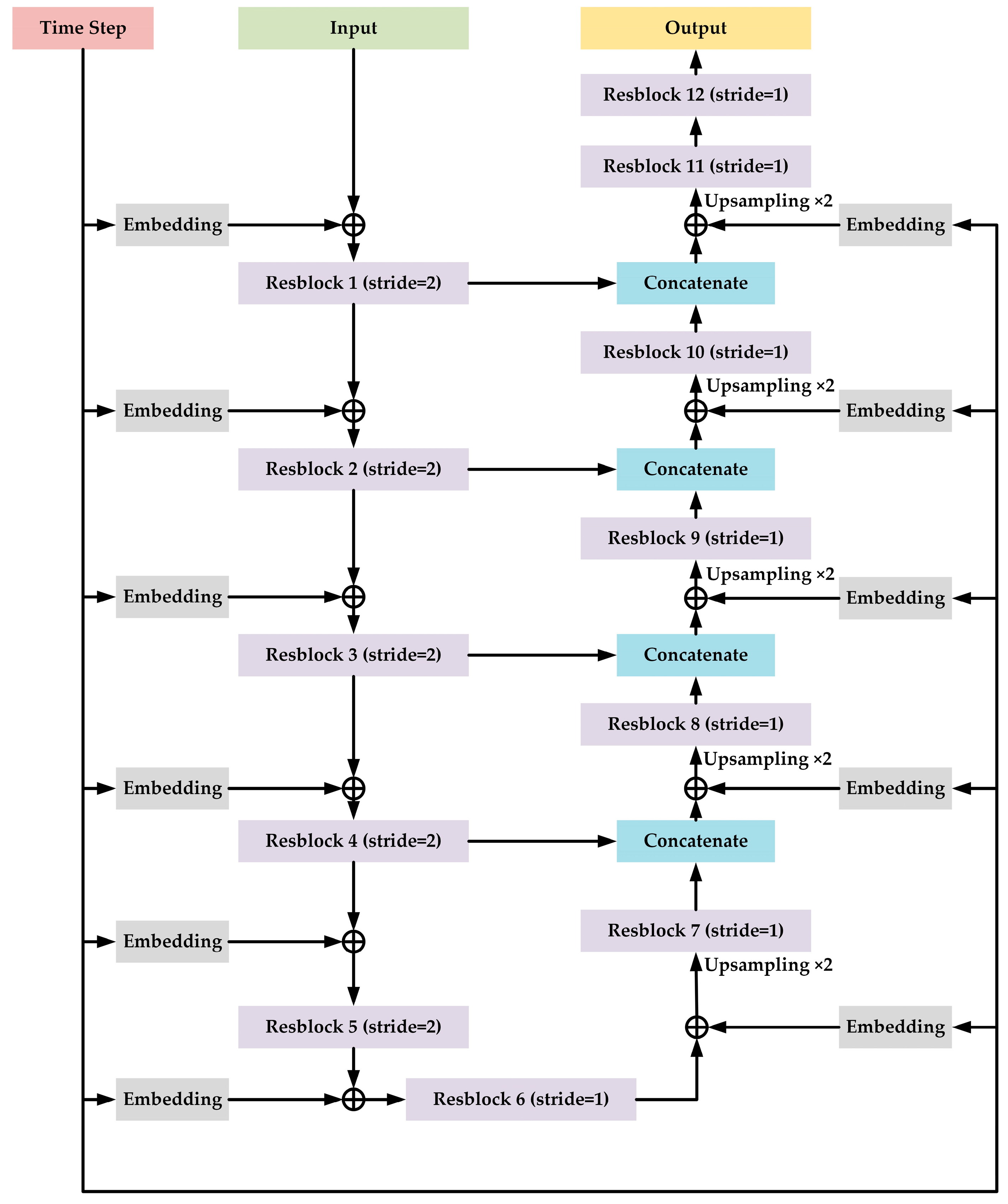
The structure of the proposed U-Net model for denoising is shown in Figure 2.

Figure 2.
The structure of the proposed U-Net model for denoising.
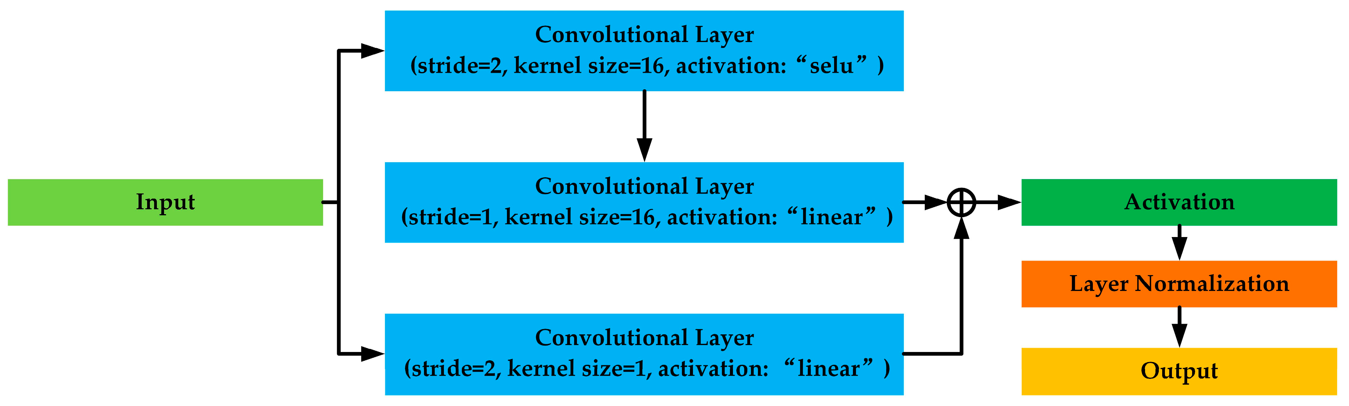
The proposed U-Net model is based on 1-D CNN, which takes the 1-D time-domain radar emitter signal sequence as input. The model contains 12 Resblocks and the structure of the Resblock is shown in Figure 3.
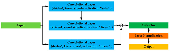
Figure 3.
The structure of the Resblock.
The Resblock is based on same structure of ResNet [32]. Each Resblock contains a short connection part and a trunk part. The short connection part includes one 1-D convolution layer, whose kernel size is 1 with a “linear” activation function and the step size is set to a certain value (we will introduce this later). The trunk part contains two cascaded 1-D convolutional layers, where the kernel size is 16 and 1, respectively. The activation functions for two 1-D convolutional layers are “selu”, which stands for “scaled exponential linear unit” [33], and “linear”, respectively, and the step size is set to a certain value (we will introduce this later) and 1. Then, an addition operation is employed to fuse two output results from the short connection part and the trunk part. Next, the result of addition operation will be activated by “selu” function. After that, layer normalization [34] is used to normalize the according result.
For Resblock 1 to Resblock 5, the step size mentioned to have a certain value is set to 2. Therefore, the output length of the corresponding Resblock is half of the input length of the corresponding Resblock. For the rest of Resblocks, the step size is set to 1. And, before sending the features from Resblock 7 to Resblock 11, the up-sampling operation, where the rate is set to be 2, is applied. Therefore, the length of the final output is same as that of the original input. Moreover, in Resblock 12 (the last Resblock), we delete the layer normalization and the subsequent activation function “selu” is changed to “linear”.
According to the design ideas of U-Net, we employ connection to some of the Resblocks; that is, the output of Resblock 1, 2, 3, and 4 is concatenated with the output of Resblock 10, 9, 8, and 7, respectively.
Moreover, as the input shape for each Resblock is different, the embedding blocks are designed independently to convert the time step to high-dimensional features. The high-dimensional features are added to different part of the proposed model.
The channel number of Resblock 1 to Resblock 12 is 64, 128, 128, 256, 256, 256, 256, 128, 128, 64, 64, and 1, respectively. Note that this U-Net-structure-based model with time embedding is only aiming for denoising. The classification models will be introduced in Section 3.3 in detail.
2.3. SNR Estimation
For our proposed U-Net model based on DDPM, the SNR of the signal waiting to be denoised has an impact on the value of the original time step to the reverse process. The sampler samples the radar emitter signal, not only the pulse part, but also the blank part that only contains the noise without the target signal. As the power of AWGN is stable during a period of time, the power of AWGN in the pulse part should be same as that in the blank part. By estimating the power of the full pulse part and the blank part, the SNR of the radar emitter signal could be calculated. The process could be written as follows:
where: is the sampled pulse part with length of , and is the sampled blank part which only contains the AWGN with length . and refer to the power of and , respectively.
2.4. Data Preprocessing
For the received time-domain sequence radar emitter signals in dataset, although some of the samples are in same SNR condition, their amplitude may different. Therefore, it is necessary to normalize the amplitude of the samples.
For convenience, we define the SNR with a 1 dB interval, where the mid value of each corresponding interval is an integer in “dB”. For example, SNR = 5 dB means that the actual SNR belongs to [4.5 dB, 5.5 dB). Based on the above rule, we could define the SNR for each sample. For example, if the actual estimated results are −4.3 dB, −4.9 dB, and 6.4 dB, then the defined SNR results are −4 dB, −5 dB, and 6 dB, respectively. As we have already known the SNR of the sample and the definition of SNR is a ratio, which means that the received signals with different power may have the same SNR due to different power of AWGN in the environment, we choose to normalize the sample, where the power of the pure signal without AWGN is set close to 0.5.
The normalization for the samples could be written as follows:
where is the defined SNR, whose value is an integer in “dB”. is the normalization result of the sampled time-domain pulse sequence with length of .
3. Dataset and Experimental Settings
In this section, we generate a simulation dataset which contains 11 different types of intra-pulse modulation. In order to show the effectiveness of our proposed denoising method, we split the dataset according to different conditions, and the description is provided in detail. We develop three DNN classification models, which take the time-domain sequences, frequency-domain sequences, and TFIs as the input, respectively, as the baseline classification methods, and the structure of these model will be illustrated. In addition, the CDAE is chosen as the baseline denoising method.
The program is based on a computer with the following specifications: Intel 10900K, 128 GB RAM, RTX 4090 GPU, MATLAB 2021a, Keras 2.3.1 and Python 3.7.
3.1. Radar Emitter Signal Intra-Pulse Modulation Dataset
In this paper, 11 types of intra-pulse modulation signals were chosen in the dataset, which include single-carrier frequency (SCF) signals, linear frequency modulation (LFM) signals, sinusoidal frequency modulation (SFM) signals, quadratic frequency modulation (EQFM) signals, dual linear frequency modulation (DLFM) signals, multiple linear frequency modulation (MLFM) signals, binary frequency shift keying (BFSK) signals, quadrature frequency shift keying (QFSK) signals, binary phase shift keying (BPSK) signals, Frank phase-coded (Frank) signals, and composite modulation with LFM and BPSK (LFM-BPSK) signals. These 11 types of modulations are more typical and widely used in radar emitter signals.
Although the carrier frequency of a radar emitter signal could range from 300 MHz to 300 GHz, the receiver of radar systems, whose local oscillators will down-mix the frequency, can output the signal sequences with a lower frequency. For example, an LFM signal sent from the emitter at 8200 MHz to 8220 MHz (in 20 MHz bandwidth) could have its frequency be down-mixed by the local oscillators of receivers. Then, the output LFM signal could be in the range of 30 MHz to 50 MHz (in 20 MHz bandwidth). Therefore, in this paper, we focus on the output signals from the receiver. Based on the above reasons, we design the dataset as follows.
The pulse width ranges from 5 us to 20 us. Assuming that the bandwidth of the receiver is 100 MHz, which is adequate for covering the bandwidth widely used for typical radar emitter signals, based on the Nyquist sampling theorem, we choose single-channel sampling with a 200 MHz sampling frequency. The parameters of the 11 intra-pulse modulations are shown in Table 1.

Table 1.
Parameters for 11 different intra-pulse modulations of radar emitter signals.
The type of noise is AWGN. The actual SNR for each modulation ranges from −10.5 dB to 10.5 dB. Based on the defined SNR in Section 2.4, there are 21 points of the defined SNR from −10 dB to 10 dB. In the rest of paper, unless otherwise specified, the SNR refers to the defined SNR in Section 2.4.
The number of samples for each modulation at each SNR is 250, where 100 samples, 50 samples, and 100 samples are used for forming the training dataset, validation dataset, and testing dataset, respectively.
3.2. Description of the Experiments with Different Conditions
In order to show the effectiveness of our proposed denoising method, we split the dataset according to different conditions. Specifically, we take three main conditions into consideration and they are shown as follows:
Condition 1.
Samples whose SNR is in the range of −10 dB to 0 dB are chosen to make the resulting training dataset, validation dataset, and testing dataset.
Condition 2.
Samples whose SNR is in the range of −10 dB to 5 dB are chosen to make the resulting training dataset, validation dataset, and testing dataset.
Condition 3.
Samples whose SNR is in the range of −10 dB to 10 dB are chosen to make the resulting training dataset, validation dataset, and testing dataset.
3.3. Baseline DNN Classification Models for Classification
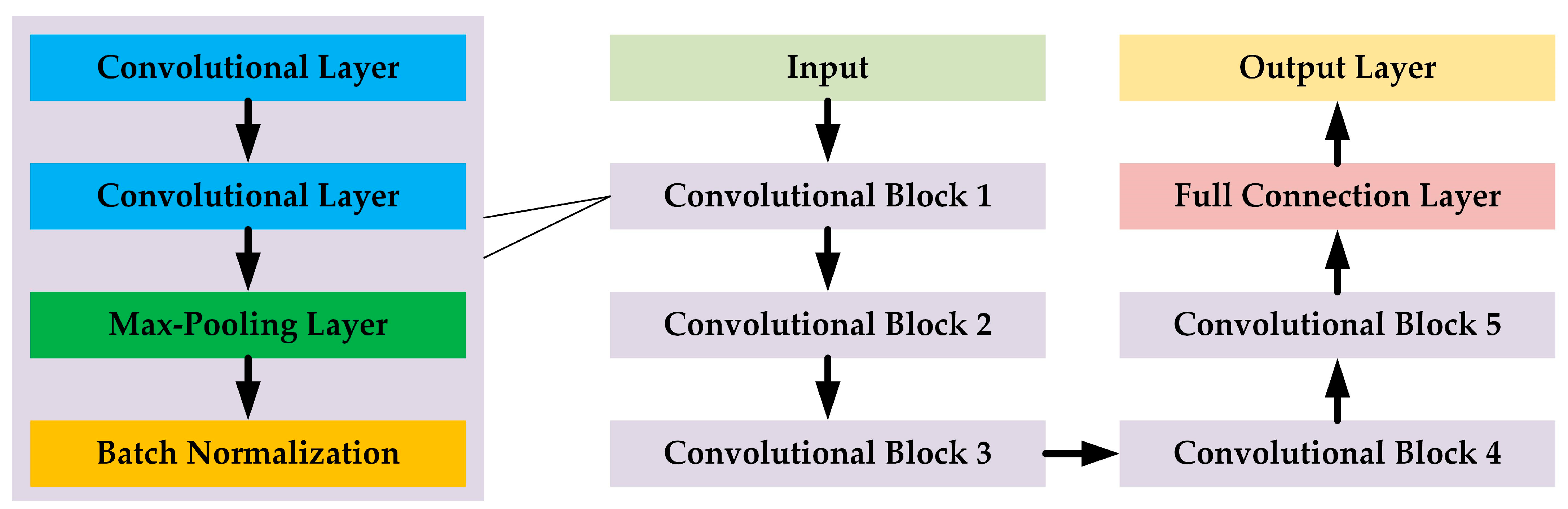
We design three representative DNN classification models based on the structure of the VGG [35], which take the time-domain sequences, frequency-domain sequences, and TFIs as the input, respectively. The main structure of these three classification models is shown in Figure 4.
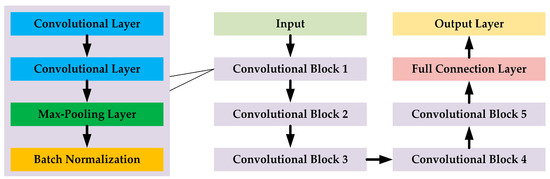
Figure 4.
The main structure of the time-domain-sequence-based, the frequency-domain-sequence-based, and the TFI-based classification models. Although the input shape and the dimensions for the convolutional blocks for these models are slightly different, all of these three models follow the same basic structure.
The three models follow the same design ideas, where each model contains five cascaded convolutional blocks, a full connection layer, and an output layer. Each convolutional block consists of two cascaded convolutional layers, a max-pooling layer, and a batch normalization layer [36]. The number of channels in each convolutional block is the same and the channels are 16, 32, 64, 128, and 256 for Convolutional Block 1 to Convolutional Block 5, respectively. The nodes of the full connection layer and the output layer are 256 and 11, respectively. Except for the output layer using the “softmax” activation function, the other related layers use the “selu” activation function.
“Adam” [37] is chosen as the optimization algorithm. The learning rate is set to be 0.001. Categorical cross-entropy is used as the loss function. The weights for the testing sections were chosen to have the highest overall recognition accuracy on the corresponding validation dataset.
For the time-domain-sequence-based and frequency-domain-sequence-based DNN classification models, they are 1-D CNN, where the kernel size in the model is set to be 16. The pooling size and step sizes are [4,4], [4,4], [4,4], [2,2], and [2,2] for Convolutional Block 1 to Convolutional Block 5, respectively. The input length for the time-domain-sequence-based DNN classification and the frequency-domain-sequence-based DNN classification is 4000 and 4096, respectively. The training epochs for the two models is 400.
The data preprocessing for the time-domain-sequence-based DNN classification model is the same as [7], where the time-domain sequences are padded with zero so that the length of all the sequences is same, at 4000. Then, the padded sequence is normalized as follows:
where is the padded time-domain sequence with a length of 4000. refers to the calculation of the absolute value of the given vector. refers to the max value obtained of the given vector. refers to the input data for the time-domain-sequence-based DNN classification model.
The data preprocessing for the frequency-domain-sequence-based DNN classification model is the same as [10], where fast Fourier transformation (FFT) with 4096 points is applied to convert the time-domain sequence to the frequency domain. By calculating the modulus of the complex frequency-domain sequence and normalizing it as follows, the input data for the frequency-domain-sequence-based DNN classification model could be obtained.
where is modulus of the complex frequency-domain sequence based on 4096-point FFT.
For the TFI-based DNN classification model, it is a 2-D CNN, where the kernel size in the model is set to be 3 × 3. The pooling size and step size for all convolutional blocks are [(2 × 2), (2 × 2)]. The input shape for the TFI-based classification DNN is 128 × 128. The training epochs for this model is 100.
The data preprocessing for the TFI-based DNN classification model is the same as [15], which is based on STFT. The normalization method is the Max–Min normalization.
3.4. CDAE Model
The CDAE is a special auto-encoder. It is widely used for image processing. In [22], the authors use the CDAE to denoise the signals in the poor SNR condition. Although the model structure and the source signal are not the same, the ideas of the CDAE are still instructive. We redesign the CDAE model, which deletes the time-embedding part of our proposed U-Net model in Section 2.2. That is to say, the denoising process in the CDAE method is one-step, while, in our method, it is multi-step, controlled by the time step. For other parameter settings, the CDAE is the same as our proposed model.
4. Experiment
4.1. Parameter Setting for Denoising U-Net Model
In a real environment, it is not possible to obtain a pure signal without AWGN. Therefore, we set three conditions in Section 3.2. For each condition, we only select the samples with the highest SNR to train our proposed denoising U-Net model.
First, we give the value of in Section 2.1 as follows:
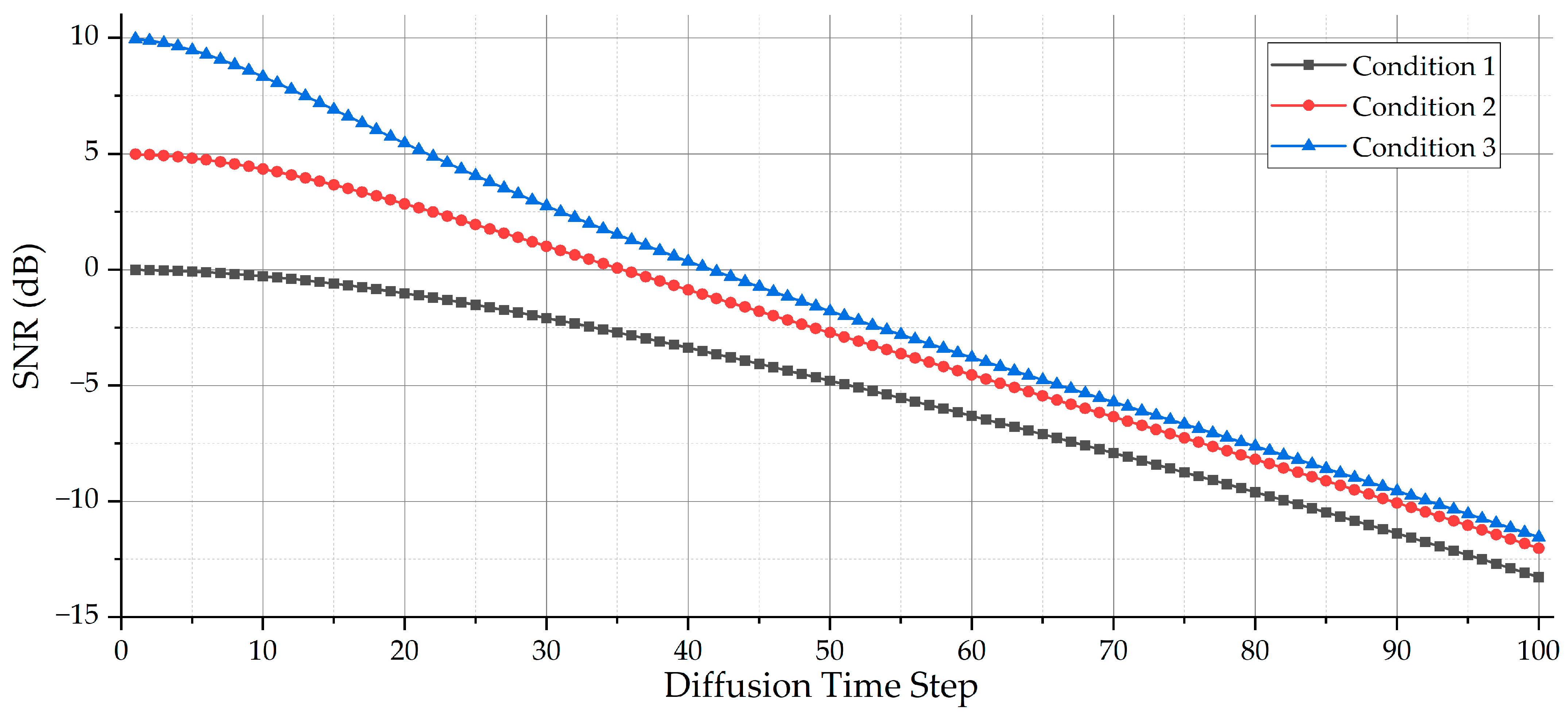
where the is the max time step of the forward process; in this paper, we set . With the forward process, the selected samples with a high SNR from the three conditions in Section 3.2 will be diffused by adding AWGN. Figure 5 shows the SNR tendency with different diffusion time steps.
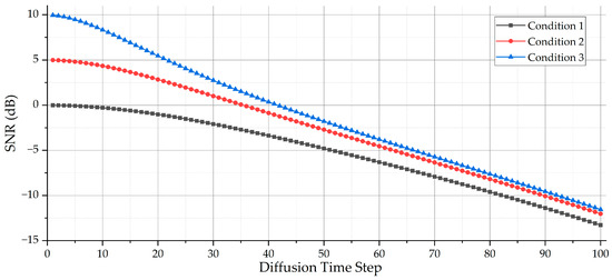
Figure 5.
The SNR tendency with different diffusion time steps based on the given . When the diffusion time step is 0, the SNR of the samples is the original value. As the diffusion time step increases, the SNR of the samples diffused by adding AWGN decreases, and, finally, the values of the SNR are at least lower than −11 dB.
It could be noticed that the start of the SNR tendency is different, as the highest SNRs of the three conditions are not the same. For Condition 1, the highest SNR is 0 dB, while, for Condition 3, the highest SNR is 10 dB. When the diffusion time step increases close to the end, the SNR tendency for all is at least lower than −11 dB.
As the length of the samples ranges from 1000 to 4000, we pad 0 to the end of each normalized sample to ensure that all the padded samples are the same length. Therefore, the input length of the denoising U-Net in Section 2.2 is 4000. Through the forward process, we could generate the resulting training dataset and the resulting validation dataset for training our denoising U-Net model.
The training epoch is set to be 400, where “Adam” [37] is used as the optimization algorithm. The learning rate is set to be 0.001. L2-distance is used as the loss function. The weights which are used for the reverse process are the weights which have the lowest L2-distance for the resulting validation dataset.
After training the denoising U-Net model well for each condition, the reverse process will be conducted. Except for the selected samples for training the denoising U-Net model, the rest of the samples, including the training samples and validation samples, will be sent to the well-trained denoising model. As the samples have different SNRs, the certain time step for the samples are different. Based on the SNR tendency with different diffusion time steps, we can find the closest time step to the sample with its SNR. After ensuring the certain time step in Section 2.2, the padded normalized sample needs to be multiplied with . Then, the result can be sent to the reverse process.
After the samples are sent to the reverse process, we only keep the part that originally contains the signal, which has the same length as its original time-domain sequence. Accordingly, the data preprocesses for the DNN classification models in Section 3.3 are all based on these signals.
Table 2 shows the certain time step for the reverse process in Section 2.2 for samples with different SNRs in Condition 1 to Condition 3, where the selected samples for training our denoising method do not participate in the reverse process. For example, in Condition 1, the samples with an SNR of 0 dB are used for training the proposed denoising U-Net based on the DDPM. For the rest of the samples in −10 dB, −9 dB, −8 dB, −7 dB, −6 dB, −5 dB, −4 dB, −3 dB, −2 dB, and −1 dB, respectively, the resultant certain time step, which is also the starting step for carrying out the reverse process based on the well-trained denoising U-Net based on the DDPM, is 82, 77, 71, 64, 58, 51, 45, 37, 29, and 20, respectively.
Table 2.
The certain time step for reverse process in Section 2.2 for samples with different SNRs in Condition 1 to Condition 3.
For the testing session, the original testing samples are all first preprocessed based on Section 2.4. Then, for the CDAE and our method, the preprocessed testing samples need to be denoising accordingly.
4.2. Classification Results
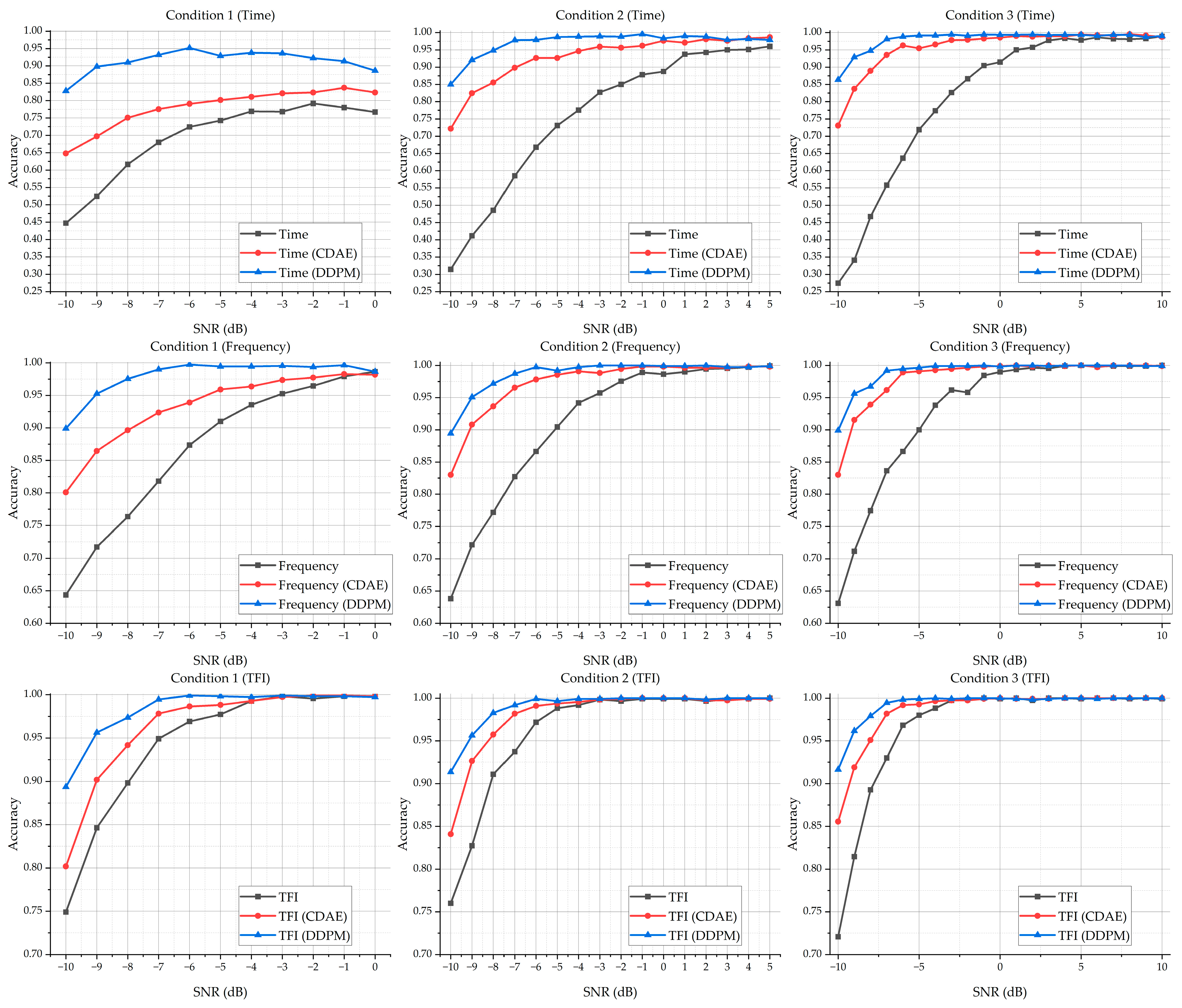
The classification accuracy of the models based on the dataset without a denoising process, with a denoising process by the CDAE, and with a denoising process by our proposed U-Net method is shown in Figure 6. Note that the transformation process for these frequency-domain sequences and the TFIs is based on the relevant undenoised or the denoised time-domain data by the CDAE and our method. For more details on the experimental results, please see Table A1, Table A2 and Table A3 in Appendix A.
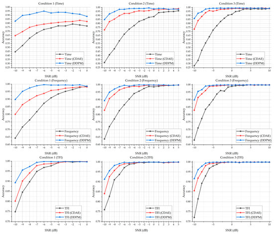
Figure 6.
The accuracy of the DNN classification models based on the dataset without a denoising process, with a denoising process by CDAE, and with a denoising process by our proposed U-Net method.
It could be noted that, without carrying out a denoising operation on the dataset, the time-domain-sequence-based DNN classification model performs extremely poorly when the SNR is low. Moreover, it also indicates that the time-domain-based DNN classification model is not stable, where the classification accuracy for the samples of Condition 1 with a lower SNR and for the samples of Condition 3 with a lower SNR are varying. The other two classification models that take the frequency-domain sequence and the TFIs as the input perform better, especially the TFI-based model, which demonstrates better accuracy when classifying the samples with a lower SNR.
It can also be seen that, with a denoising process by the CDAE, the accuracy of the three DNN classification models increases. In some conditions, even, the performance of the time-domain-sequence-based DNN classification model can compete with the original frequency-domain-based DNN classification model and the original TFI-based DNN classification model. Compared with the original DNN classification models without a denoising process, all three models trained by the denoised data with the CDAE could classify the resulting samples in a lower SNR condition with better accuracy.
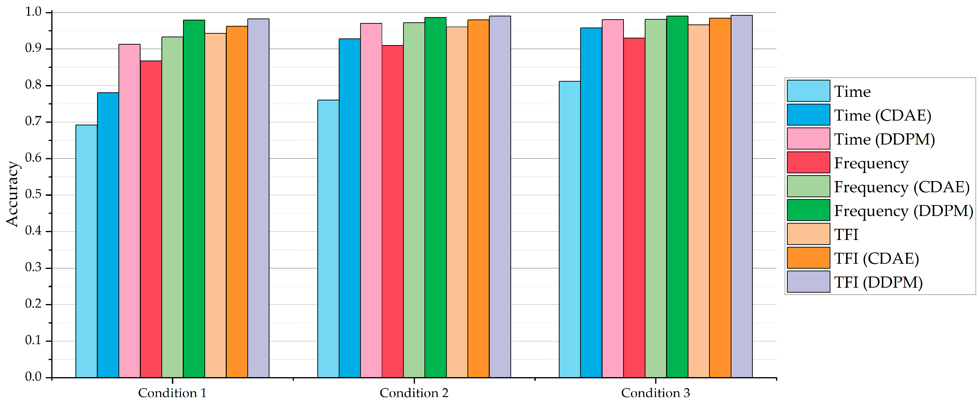
Meanwhile, it could be noticed that, trained with the data based on our proposed U-Net method, even the time-domain-sequence-based DNN classification model could classify the samples at −10 dB with over 80% accuracy. In these conditions, its performance could be better than the original frequency-domain-based DNN classification model, and even the original TFI-based DNN classification model. Compared with the classification models with a denoising process by the CDAE, the classification models with our method’s denoising process perform better, where the global average accuracy for each condition is over 90%. Figure 7 shows the average classification accuracy based on the DNN classification models for Condition 1 to Condition 3.
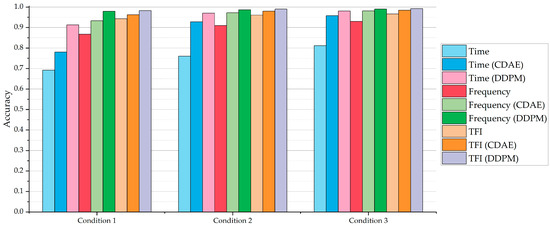
Figure 7.
The average accuracy based on three types of DNN classification models with Condition 1 to Condition 3.
Figure 7 indicates that, in the three different conditions, both the CDAE denoising method and our denoising method can increase the performance of the DNN classification models. In terms of the results based on the time-domain-sequence-based classification DNN model, it can be found that our denoising method is better than the CDAE denoising method, where the average classification accuracy is improved by about 15 to 20 percentage points.
Meanwhile, the relevant DNN classification models, which are trained with the resulting frequency-domain sequences and the resulting TFIs that are transformed by the denoised time-domain sequences with the CDAE denoising method, demonstrate better accuracy than those trained with the data without a denoising process. Although, for the frequency-domain-sequence-based DNN classification model and TFI-based DNN classification model, the average classification accuracy is not improved by as much as that of the time-domain-sequence-based DNN classification model, the effectiveness of the denoising process based on our method is still obvious.
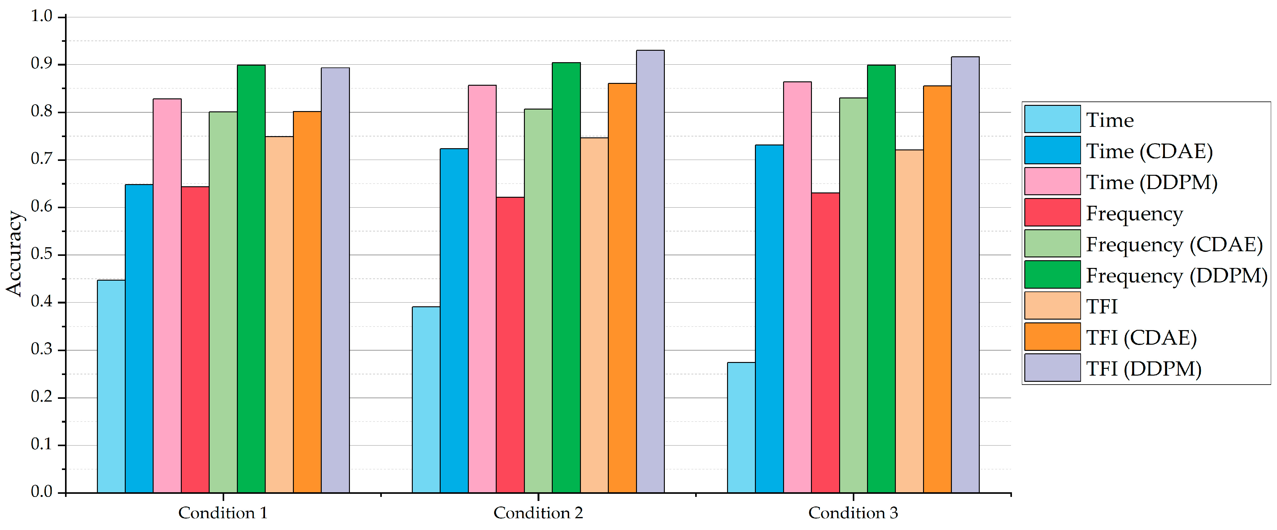
Figure 8 shows the accuracy of the DNN classification models for the samples with an SNR of −10 dB in Condition 1 to Condition 3 without a denoising process, with a denoising process by the CDAE, and with a denoising process by our method, respectively. It could be noted that, when denoising by our method, the relevant DNN classification models have been greatly improved compared to those without a denoising process.
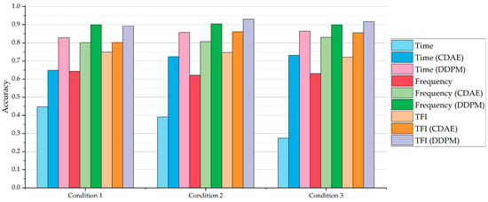
Figure 8.
The accuracy of the DNN classification models for the samples with SNR of −10 dB in Condition 1 to Condition 3 without a denoising process, with a denoising process by CDAE, and with a denoising process by our method, respectively.
In addition, it could be seen that, for each condition, the accuracy of the resultant DNN classification model generally improves with the increment in the SNR. Therefore, in order to analyze the effectiveness of the denoising process, we set an accuracy threshold of 90% for the three conditions. Table 3 shows the lowest value of the SNR for each condition that meets the accuracy threshold of 90% or more.
Table 3.
The lowest value of SNR for each condition that meets the accuracy threshold of 90% or more. “N/A” means that, in this condition, the highest accuracy of the samples based on this classification model in any point of SNR is lower than 90%. For example, in Condition 1, the highest accuracy of the samples based on the time-domain-sequence-based DNN classification model without a denoising process in any point of SNR is lower than 90%.
Note that, although in some conditions like Condition 1, based on the DNN classification model with a denoising process by our method, the accuracy for some samples with a lower SNR is higher than those with a higher SNR; generally, the tendency of the accuracy rises when the value of the SNR increases. As a result, the lowest value of the SNR for the relevant DNN classification model in this Condition 1 is chosen to be −8 dB.
Table 3 illustrates that, for the DNN classification models with the same modal input, generally, both the CDAE and our method can make the accuracy based on the relevant classification models for the samples with a lower value SNR meet the accuracy threshold of 90%. For example, in Condition 3, only the accuracy for the samples that are greater than or equal to −1 dB based on the time-domain-sequence-based DNN classification model can reach the threshold of 90%. When a denoising process is employed, the minimum SNR that meets the accuracy threshold based on the relevant time-domain-sequence-based DNN classification model is reduced to −7 dB by the CDAE and −9 dB by our U-Net method, respectively. Meanwhile, it can be seen that the improvement based on our denoising method is better than that based on the CDAE method, especially when the classification models are trained with time-domain sequences.
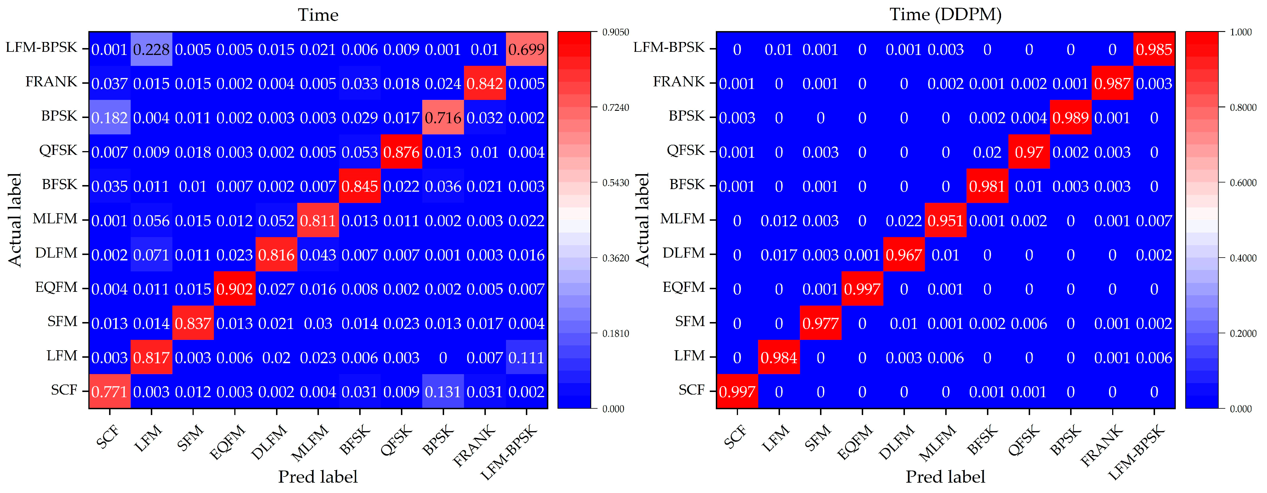
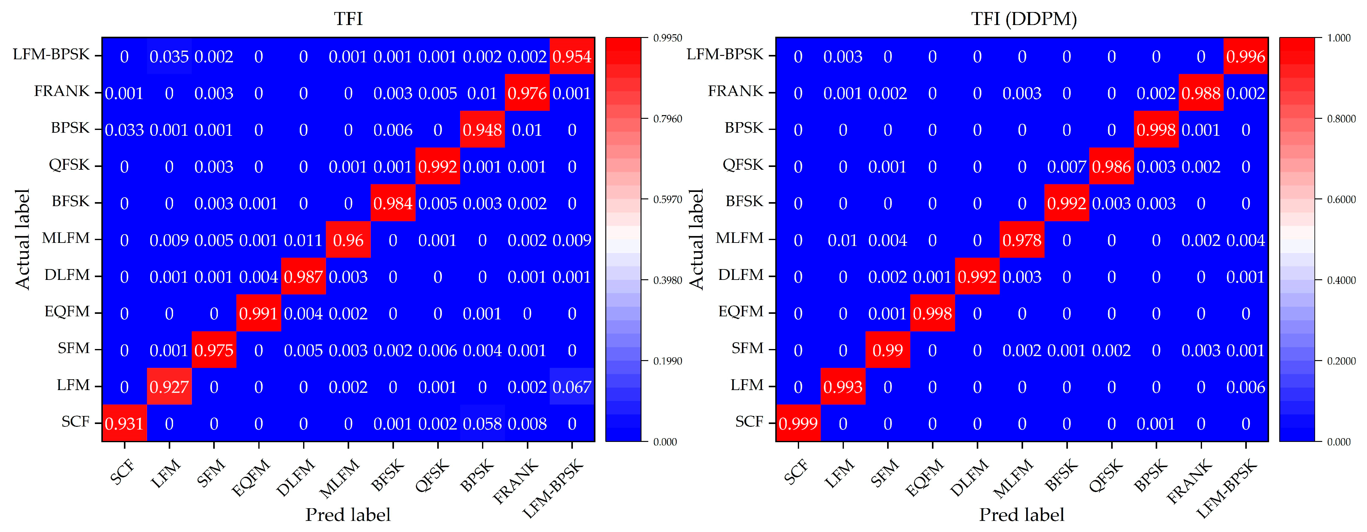
To further evaluate the performance of the DNN classification models without and with a denoising process by our method, we focus on the confusion matrix for the 11 different intra-pulse modulations with the DNN classification models in Condition 3, where this condition can represent a general situation in real environments. Figure 9, Figure 10 and Figure 11 show the confusion matrices of the relevant DNN classification models based on Condition 3, which take the time-domain sequences, frequency-domain sequences, and TFIs as the input, respectively.
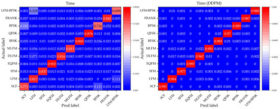
Figure 9.
The confusion matrix of the time-domain-sequence-based DNN classification models without and with a denoising process by our method for the 11 different intra-pulse modulations in Condition 3.
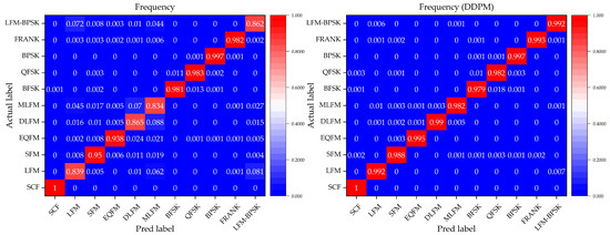
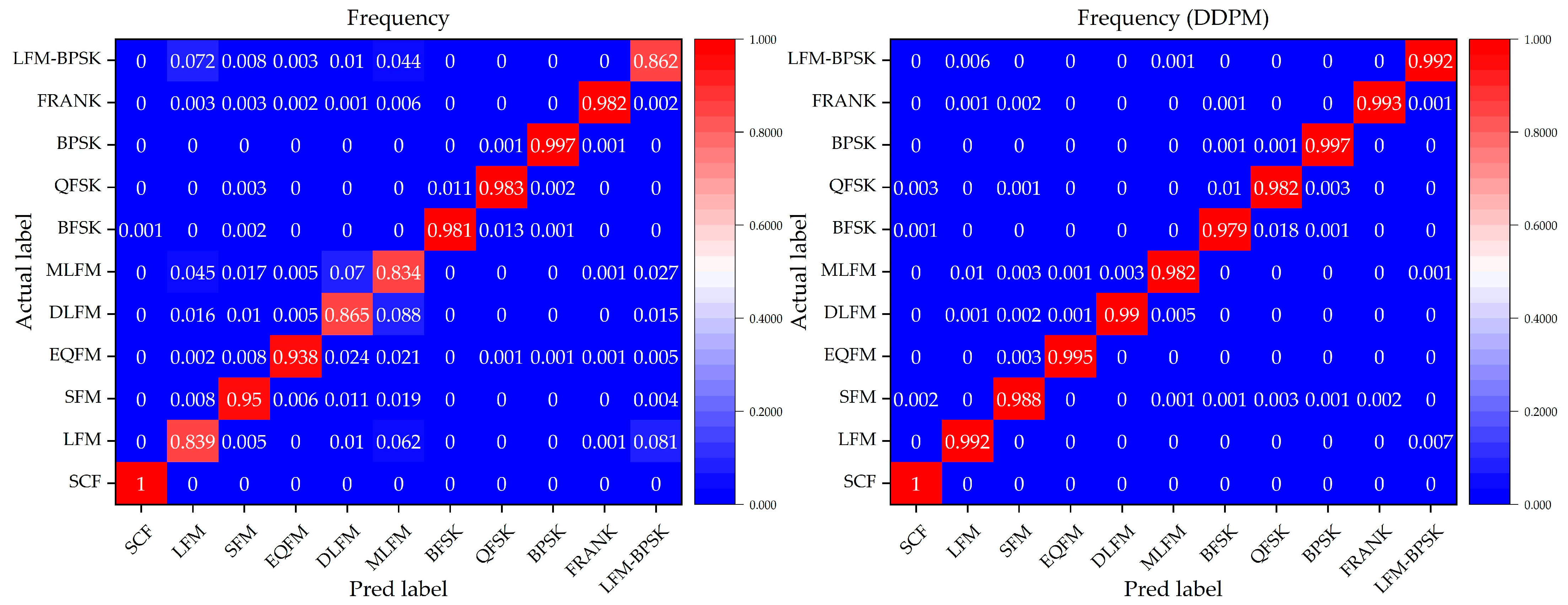
Figure 10.
The confusion matrix of the frequency-domain-sequence-based DNN classification models without and with a denoising process by our method for the 11 different intra-pulse modulations in Condition 3.
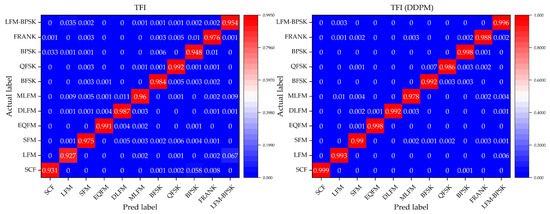
Figure 11.
The confusion matrix of the TFI-domain-sequence-based DNN classification models without and with a denoising process by our method for the 11 different intra-pulse modulations in Condition 3.
It is indicated that, for the 11 different intra-pulse modulations, our method increases the classification accuracy. From the confusion matrices, it can be seen that the DNN classification models without a denoising process cannot classify some intra-pulse modulations as well as others, like LFM samples and LFM-BPSK samples. However, with our denoising method, the DNN classification models can overcome their weakness in classifying the above-mentioned intra-pulse modulations. For example, the ratio of the confusion pairs of LFM and LFM-BPSK, and SCF and BPSK in the time-domain-sequence-based DNN classification model, are greatly suppressed with the usage of our denoising method. Taking a comprehensive look at the performance on classifying 11 modulations, our method is effective and can further improve the accuracy of all three DNN classification models.
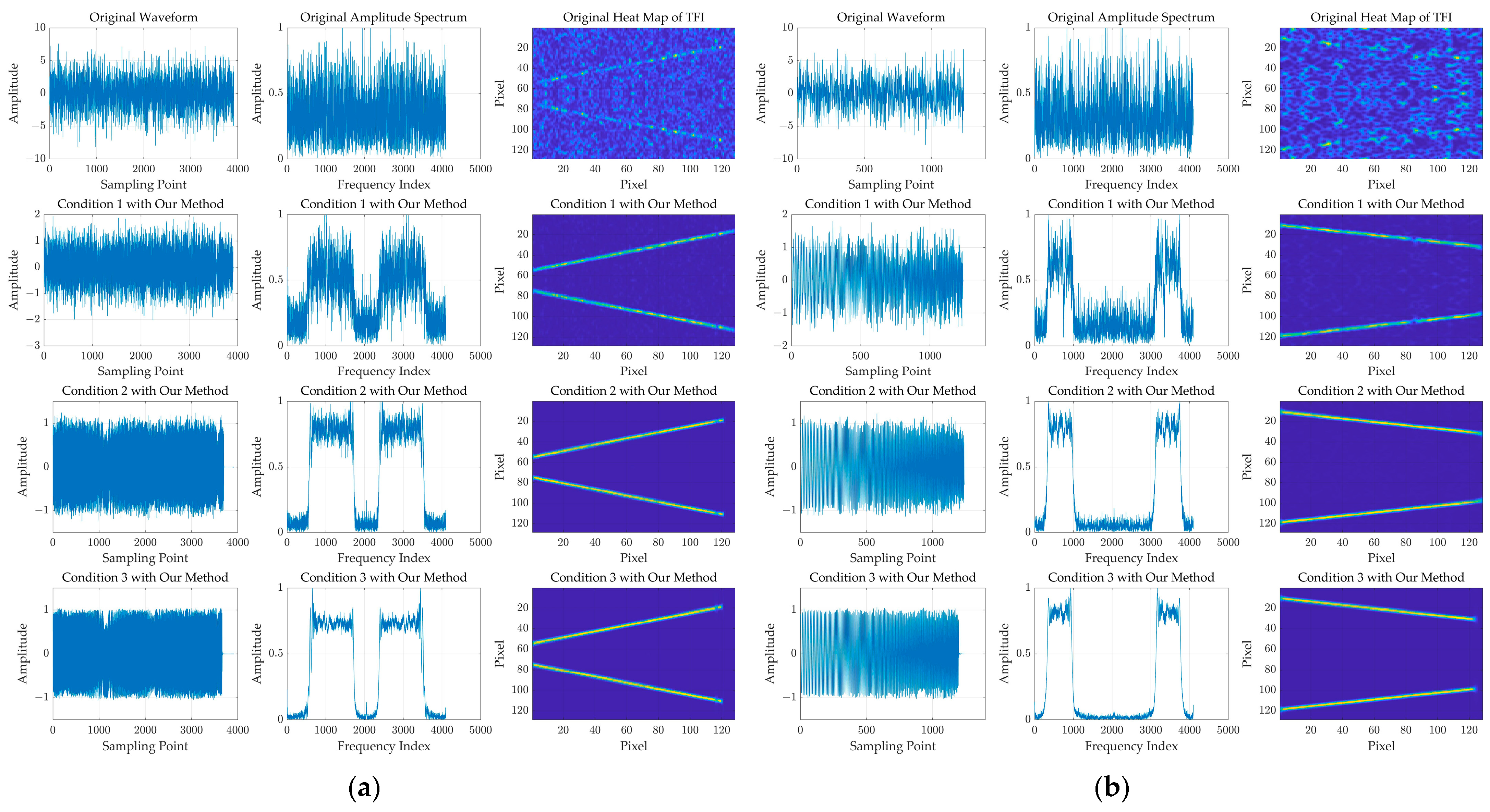
Figure 12 shows a denoising result based on our denoising method for two LFM samples in Condition 1, Condition 2, and Condition 3, respectively, where the two LFM samples are have a −10 dB SNR.

Figure 12.
The denoising result based on our denoising method for two LFM samples with −10 dB SNR in Condition 1, Condition 2, and Condition 3, respectively. (a) is the relevant result for the first LFM sample. (b) is the relevant result for the second LFM sample. The columns from left to right represent the waveform, the amplitude spectrum, and the heat map of TFI, respectively.
For our method based on the DDPM, it could be found that, through the denoising process, some parts of the sample may be over-denoised, like the small part at the end of the signal, where the model outputs the resulting parts with a value of approximately “0”. However, the denoising effect based on our method is stable, generally. Moreover, it could be noted that, if choosing a sample with a higher value of SNR to train our denoising model, the denoising effect will be better.
As a result, based on the extensive experimental results with the three different conditions, it is indicated that our proposed method can denoise and increase the quality of the signal so that, trained with the denoised signals and denoising the signal to be classified, the classification models can effectively increase their accuracy for intra-pulse modulations.
5. Discussion
5.1. Ablation Study on the Max Time Step of Forward Process
We analyze the influence of the max time step of the forward process setting on signal denoising. Specifically, we conduct the denoising methods when the value of is 25, 50, and 200 (the experiment with could be seen in Section 4.2). Based on the resulting denoised samples, we train and test the resulting DNN classification models. The set of based on the above value of is shown as follows.
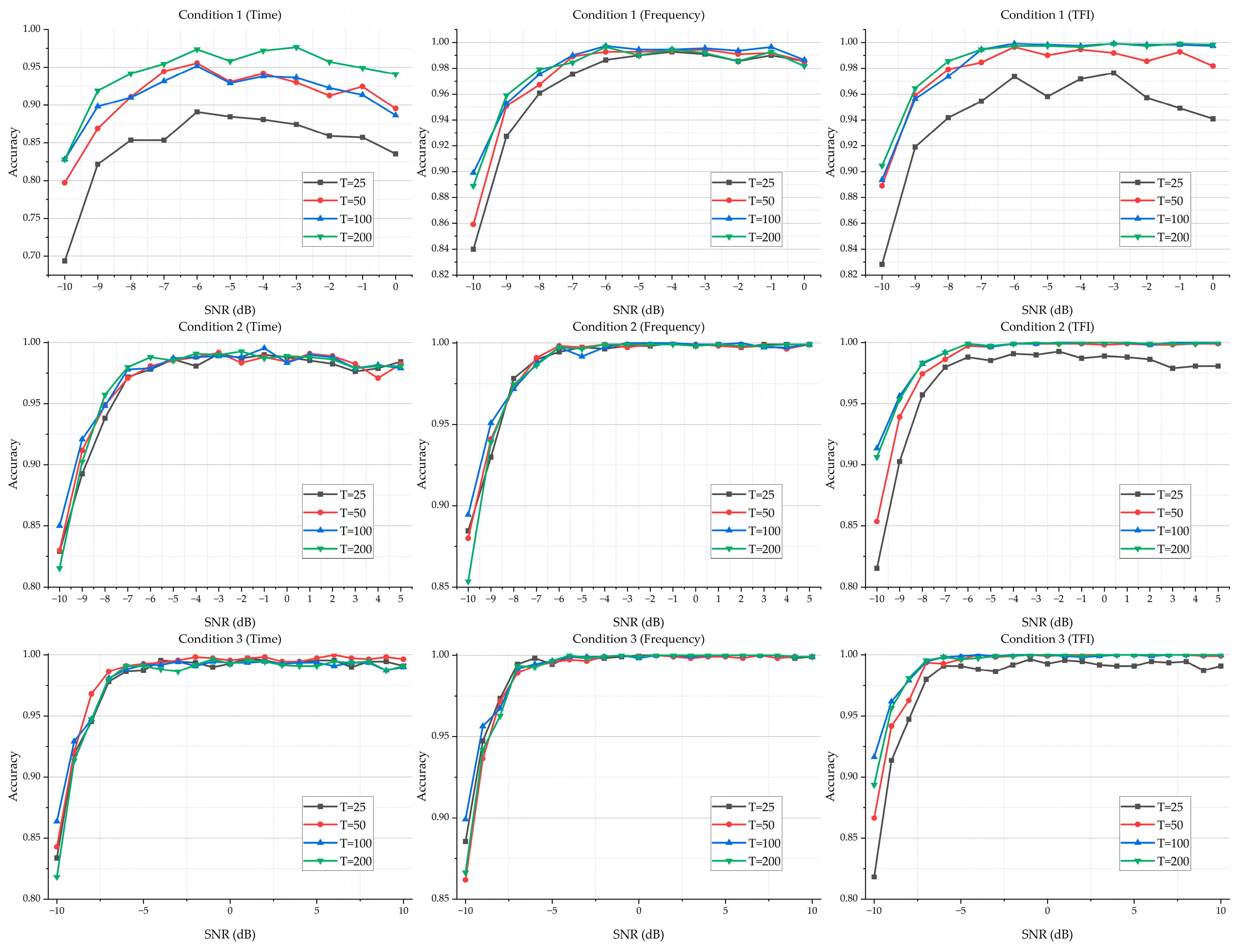
Under a different value of , the classification results of the time-domain-sequence-based DNN classification models, frequency-domain-sequence-based DNN classification models, and TFI-based DNN classification models in Condition 1, Condition 2, and Condition 3, respectively, are shown in Figure 13. For more details on the experimental results, please see Table A4, Table A5 and Table A6 in Appendix B.
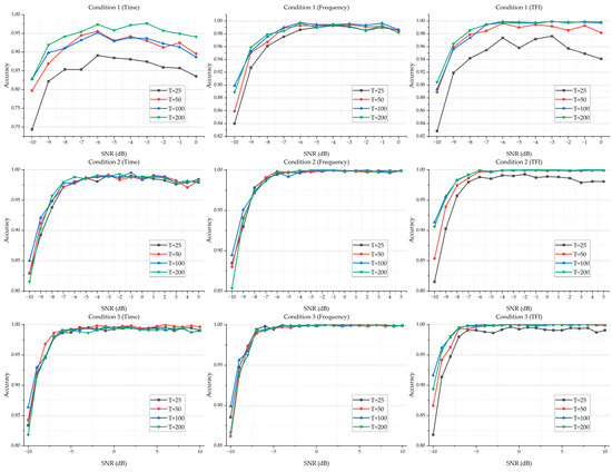
Figure 13.
The classification results of time-domain-sequence-based DNN classification models, frequency-domain-sequence-based DNN classification models, and TFI-based DNN classification models in Condition 1, Condition 2, and Condition 3, respectively, with a different value of .
It is noted that increasing the value of could improve the performance of the resulting DNN classification models. Compared with other values of , the classification models with have an obvious gap in accuracy in these conditions, where the selected samples for training the denoising U-Net model have a lower SNR (like Condition 1).
However, as the value of increases, the classification accuracy increases first and then levels off. In addition, when the selected samples for training the denoising U-Net model have a good SNR, the classification models based on a lower value of could provide a competitive or similar level of performance compared with those based on a higher value of (like Condition 3).
Moreover, although increasing the value of will improve the classification models’ performance for different conditions, the computation time will increase accordingly. For example, after training the denoising model with and based on Condition 3, the resulting certain time step of a reverse process for the sample in −10 dB is 46 and 186, where the processing time for the latter is around four times than that of the former. In this paper, taking the classification accuracy and time usage into considerations, we set the value of the max time step to 100.
5.2. Potential Application Scenarios
Through the experimental results, our proposed denoising method based on the DDPM could denoise the signal in poor SNR conditions and provide high-quality samples for the DNN classification models. Focusing on the training process of our method, it is noted that the training of the denoising method is unsupervised-like, where the source data are not manually annotated with information such as categories. Therefore, the proposed denoising method is easy to conduct as there is no traditional expensive data annotation process.
At the same time, in addition to helping to train the DNN classification models, our method is also an effective data quality improvement method, which could be used in semi-supervised classification and the open set recognition of radar emitter signal intra-pulse modulation. Moreover, our method could also be applied to other radar signal recognition and classification tasks, like radar jamming recognition tasks and specific emitter identification tasks.
6. Conclusions
In this paper, we proposed an effective denoising method based on the DDPM for radar emitter signal intra-pulse modulation classification. With the denoised samples by our method, the classification accuracies of three DNN models with the time-domain-sequence-based input, the frequency-domain-sequence-based input, and the TFI-based input improve more than with the original samples and the samples denoised by the CDAE method. Additionally, the ablation study shows that both increasing the max time step samples or selecting the samples with a higher SNR for training our proposed denoising U-Net model could help the DNN classification models perform better. Moreover, our proposed denoising method could also provide potential guidance for other radar signal recognition and classification tasks.
As our proposed denoising process is carried out step by step, in a future work, we will attempt to optimize the proposed denoising method with a faster denoising process.
Author Contributions
Conceptualization, S.Y. and P.L.; methodology, S.Y. and P.L.; software, S.Y. and Y.C.; validation, S.Y.; formal analysis, S.Y. and P.L.; investigation, S.Y.; resources, S.Y., P.L. and B.W.; data curation, S.Y.; writing—original draft preparation, S.Y.; writing—review and editing, S.Y.; visualization, S.Y. and X.Z.; supervision, P.L. and B.W.; project administration, P.L. All authors have read and agreed to the published version of the manuscript.
Funding
This research received no external funding.
Data Availability Statement
The data are contained within the article.
Acknowledgments
The authors would like to show their gratitude to the editors and the reviewers for their insightful comments.
Conflicts of Interest
The authors declare no conflicts of interest.
Appendix A
The details of the experimental results in Section 4.2 are shown in Table A1, Table A2 and Table A3.
Table A1.
The accuracy of the time-domain-sequence-based, frequency-domain-sequence-based, and TFI-based DNN classification models based on the dataset without a denoising process in Condition 1 to Condition 3.
Table A1.
The accuracy of the time-domain-sequence-based, frequency-domain-sequence-based, and TFI-based DNN classification models based on the dataset without a denoising process in Condition 1 to Condition 3.
| SNR/dB | Condition 1 | Condition 2 | Condition 3 | ||||||
|---|---|---|---|---|---|---|---|---|---|
| Time | Frequency | TFI | Time | Frequency | TFI | Time | Frequency | TFI | |
| −10 | 0.4473 | 0.6436 | 0.7491 | 0.3145 | 0.6382 | 0.7600 | 0.2745 | 0.6309 | 0.7209 |
| −9 | 0.5245 | 0.7173 | 0.8464 | 0.4118 | 0.7218 | 0.8273 | 0.3409 | 0.7118 | 0.8145 |
| −8 | 0.6164 | 0.7636 | 0.8982 | 0.4855 | 0.7718 | 0.9109 | 0.4673 | 0.7745 | 0.8927 |
| −7 | 0.6800 | 0.8182 | 0.9491 | 0.5855 | 0.8273 | 0.9373 | 0.5582 | 0.8364 | 0.9300 |
| −6 | 0.7245 | 0.8736 | 0.9691 | 0.6682 | 0.8664 | 0.9718 | 0.6364 | 0.8664 | 0.9682 |
| −5 | 0.7427 | 0.9100 | 0.9773 | 0.7309 | 0.9045 | 0.9882 | 0.7191 | 0.9000 | 0.9800 |
| −4 | 0.7691 | 0.9355 | 0.9927 | 0.7755 | 0.9418 | 0.9918 | 0.7736 | 0.9382 | 0.9882 |
| −3 | 0.7682 | 0.9527 | 0.9982 | 0.8273 | 0.9573 | 0.9982 | 0.8264 | 0.9618 | 0.9973 |
| −2 | 0.7918 | 0.9645 | 0.9955 | 0.8500 | 0.9755 | 0.9964 | 0.8664 | 0.9582 | 0.9982 |
| −1 | 0.7800 | 0.9791 | 0.9982 | 0.8782 | 0.9891 | 0.9991 | 0.9045 | 0.9845 | 1.0000 |
| 0 | 0.7673 | 0.9864 | 0.9982 | 0.8873 | 0.9864 | 0.9991 | 0.9145 | 0.9900 | 0.9991 |
| 1 | — | — | — | 0.9373 | 0.9900 | 0.9991 | 0.9500 | 0.9936 | 1.0000 |
| 2 | — | — | — | 0.9427 | 0.9945 | 0.9964 | 0.9573 | 0.9964 | 0.9973 |
| 3 | — | — | — | 0.9500 | 0.9955 | 0.9982 | 0.9773 | 0.9955 | 1.0000 |
| 4 | — | — | — | 0.9509 | 0.9973 | 0.9991 | 0.9836 | 0.9991 | 1.0000 |
| 5 | — | — | — | 0.9600 | 0.9991 | 1.0000 | 0.9782 | 1.0000 | 0.9991 |
| 6 | — | — | — | — | — | — | 0.9864 | 0.9982 | 1.0000 |
| 7 | — | — | — | — | — | — | 0.9818 | 0.9991 | 1.0000 |
| 8 | — | — | — | — | — | — | 0.9809 | 0.9991 | 0.9991 |
| 9 | — | — | — | — | — | — | 0.9827 | 0.9991 | 1.0000 |
| 10 | — | — | — | — | — | — | 0.9891 | 1.0000 | 0.9991 |
| AA | 0.6920 | 0.8677 | 0.9429 | 0.7597 | 0.9098 | 0.9608 | 0.8119 | 0.9301 | 0.9659 |
Table A2.
The accuracy of the time-domain-sequence-based, frequency-domain-sequence-based, and TFI-based DNN classification models based on the dataset with a denoising process by CDAE in Condition 1 to Condition 3.
Table A2.
The accuracy of the time-domain-sequence-based, frequency-domain-sequence-based, and TFI-based DNN classification models based on the dataset with a denoising process by CDAE in Condition 1 to Condition 3.
| SNR/dB | Condition 1 | Condition 2 | Condition 3 | ||||||
|---|---|---|---|---|---|---|---|---|---|
| Time | Frequency | TFI | Time | Frequency | TFI | Time | Frequency | TFI | |
| −10 | 0.6482 | 0.8009 | 0.8018 | 0.7218 | 0.8300 | 0.8409 | 0.7309 | 0.8300 | 0.8555 |
| −9 | 0.6973 | 0.8645 | 0.9018 | 0.8245 | 0.9082 | 0.9264 | 0.8373 | 0.9155 | 0.9191 |
| −8 | 0.7509 | 0.8964 | 0.9418 | 0.8555 | 0.9364 | 0.9573 | 0.8891 | 0.9391 | 0.9509 |
| −7 | 0.7755 | 0.9236 | 0.9782 | 0.8982 | 0.9655 | 0.9818 | 0.9355 | 0.9618 | 0.9818 |
| −6 | 0.7909 | 0.9391 | 0.9864 | 0.9264 | 0.9782 | 0.9909 | 0.9627 | 0.9891 | 0.9918 |
| −5 | 0.8018 | 0.9591 | 0.9882 | 0.9264 | 0.9855 | 0.9936 | 0.9545 | 0.9909 | 0.9927 |
| −4 | 0.8109 | 0.9636 | 0.9927 | 0.9464 | 0.9909 | 0.9955 | 0.9655 | 0.9927 | 0.9964 |
| −3 | 0.8209 | 0.9736 | 0.9973 | 0.9591 | 0.9882 | 0.9982 | 0.9782 | 0.9945 | 0.9973 |
| −2 | 0.8236 | 0.9773 | 0.9991 | 0.9564 | 0.9945 | 0.9991 | 0.9791 | 0.9964 | 0.9973 |
| −1 | 0.8373 | 0.9827 | 0.9991 | 0.9618 | 0.9982 | 1.0000 | 0.9827 | 0.9982 | 0.9991 |
| 0 | 0.8236 | 0.9818 | 0.9982 | 0.9764 | 0.9982 | 1.0000 | 0.9855 | 0.9991 | 1.0000 |
| 1 | — | — | — | 0.9709 | 0.9964 | 1.0000 | 0.9900 | 1.0000 | 0.9991 |
| 2 | — | — | — | 0.9809 | 0.9964 | 0.9973 | 0.9882 | 0.9982 | 0.9991 |
| 3 | — | — | — | 0.9764 | 0.9964 | 0.9973 | 0.9900 | 1.0000 | 0.9991 |
| 4 | — | — | — | 0.9836 | 0.9982 | 0.9991 | 0.9891 | 0.9991 | 1.0000 |
| 5 | — | — | — | 0.9864 | 0.9982 | 0.9991 | 0.9945 | 1.0000 | 1.0000 |
| 6 | — | — | — | — | — | — | 0.9927 | 0.9973 | 1.0000 |
| 7 | — | — | — | — | — | — | 0.9918 | 1.0000 | 1.0000 |
| 8 | — | — | — | — | — | — | 0.9955 | 1.0000 | 1.0000 |
| 9 | — | — | — | — | — | — | 0.9918 | 1.0000 | 1.0000 |
| 10 | — | — | — | — | — | — | 0.9873 | 0.9991 | 1.0000 |
| AA | 0.7801 | 0.9330 | 0.9622 | 0.9282 | 0.9724 | 0.9798 | 0.9577 | 0.9810 | 0.9847 |
Table A3.
The accuracy of the time-domain-sequence-based, frequency-domain-sequence-based, and TFI-based DNN classification models based on the dataset with a denoising process by our proposed U-Net method in Condition 1 to Condition 3.
Table A3.
The accuracy of the time-domain-sequence-based, frequency-domain-sequence-based, and TFI-based DNN classification models based on the dataset with a denoising process by our proposed U-Net method in Condition 1 to Condition 3.
| SNR/dB | Condition 1 | Condition 2 | Condition 3 | ||||||
|---|---|---|---|---|---|---|---|---|---|
| Time | Frequency | TFI | Time | Frequency | TFI | Time | Frequency | TFI | |
| −10 | 0.8282 | 0.8991 | 0.8936 | 0.8500 | 0.8945 | 0.9136 | 0.8636 | 0.8991 | 0.9164 |
| −9 | 0.8982 | 0.9527 | 0.9564 | 0.9209 | 0.9509 | 0.9564 | 0.9291 | 0.9564 | 0.9618 |
| −8 | 0.9100 | 0.9755 | 0.9736 | 0.9482 | 0.9718 | 0.9827 | 0.9473 | 0.9673 | 0.9791 |
| −7 | 0.9318 | 0.9900 | 0.9945 | 0.9782 | 0.9873 | 0.9918 | 0.9809 | 0.9918 | 0.9945 |
| −6 | 0.9518 | 0.9973 | 0.9991 | 0.9791 | 0.9973 | 0.9991 | 0.9882 | 0.9945 | 0.9982 |
| −5 | 0.9291 | 0.9945 | 0.9982 | 0.9873 | 0.9918 | 0.9964 | 0.9918 | 0.9964 | 0.9991 |
| −4 | 0.9382 | 0.9945 | 0.9973 | 0.9882 | 0.9973 | 0.9991 | 0.9918 | 0.9991 | 1.0000 |
| −3 | 0.9364 | 0.9955 | 0.9991 | 0.9891 | 1.0000 | 0.9991 | 0.9945 | 0.9991 | 0.9991 |
| −2 | 0.9227 | 0.9936 | 0.9982 | 0.9882 | 1.0000 | 1.0000 | 0.9909 | 0.9991 | 1.0000 |
| −1 | 0.9136 | 0.9964 | 0.9982 | 0.9955 | 1.0000 | 1.0000 | 0.9945 | 1.0000 | 1.0000 |
| 0 | 0.8864 | 0.9864 | 0.9973 | 0.9836 | 0.9991 | 1.0000 | 0.9936 | 0.9982 | 1.0000 |
| 1 | — | — | — | 0.9900 | 0.9991 | 1.0000 | 0.9936 | 1.0000 | 0.9991 |
| 2 | — | — | — | 0.9882 | 1.0000 | 0.9982 | 0.9945 | 1.0000 | 0.9982 |
| 3 | — | — | — | 0.9791 | 0.9973 | 1.0000 | 0.9927 | 0.9991 | 0.9991 |
| 4 | — | — | — | 0.9818 | 0.9973 | 1.0000 | 0.9936 | 1.0000 | 1.0000 |
| 5 | — | — | — | 0.9791 | 0.9991 | 1.0000 | 0.9936 | 1.0000 | 1.0000 |
| 6 | — | — | — | — | — | — | 0.9909 | 1.0000 | 0.9991 |
| 7 | — | — | — | — | — | — | 0.9936 | 1.0000 | 1.0000 |
| 8 | — | — | — | — | — | — | 0.9936 | 1.0000 | 1.0000 |
| 9 | — | — | — | — | — | — | 0.9873 | 0.9991 | 1.0000 |
| 10 | — | — | — | — | — | — | 0.9900 | 0.9991 | 1.0000 |
| AA | 0.9133 | 0.9796 | 0.9823 | 0.9704 | 0.9864 | 0.9898 | 0.9805 | 0.9904 | 0.9926 |
Appendix B
The details of the experimental results in Section 5.1 are shown in Table A4, Table A5 and Table A6.
Table A4.
The accuracy of the time-domain-sequence-based, frequency-domain-sequence-based, and TFI-based DNN classification models based on the dataset with a denoising process by our proposed U-Net method in Condition 1 to Condition 3 when the value of is set to be 25.
Table A4.
The accuracy of the time-domain-sequence-based, frequency-domain-sequence-based, and TFI-based DNN classification models based on the dataset with a denoising process by our proposed U-Net method in Condition 1 to Condition 3 when the value of is set to be 25.
| SNR/dB | Condition 1 | Condition 2 | Condition 3 | ||||||
|---|---|---|---|---|---|---|---|---|---|
| Time | Frequency | TFI | Time | Frequency | TFI | Time | Frequency | TFI | |
| −10 | 0.6936 | 0.8400 | 0.8282 | 0.8291 | 0.8845 | 0.8155 | 0.8336 | 0.8855 | 0.8182 |
| −9 | 0.8218 | 0.9273 | 0.9191 | 0.8927 | 0.9300 | 0.9027 | 0.9191 | 0.9473 | 0.9136 |
| −8 | 0.8536 | 0.9609 | 0.9418 | 0.9382 | 0.9782 | 0.9573 | 0.9455 | 0.9736 | 0.9473 |
| −7 | 0.8536 | 0.9755 | 0.9545 | 0.9718 | 0.9900 | 0.9800 | 0.9782 | 0.9945 | 0.9800 |
| −6 | 0.8909 | 0.9864 | 0.9736 | 0.9782 | 0.9945 | 0.9882 | 0.9864 | 0.9982 | 0.9909 |
| −5 | 0.8845 | 0.9900 | 0.9582 | 0.9864 | 0.9973 | 0.9855 | 0.9873 | 0.9945 | 0.9909 |
| −4 | 0.8809 | 0.9927 | 0.9718 | 0.9809 | 0.9964 | 0.9909 | 0.9955 | 0.9991 | 0.9882 |
| −3 | 0.8745 | 0.9909 | 0.9764 | 0.9909 | 0.9982 | 0.9900 | 0.9945 | 0.9982 | 0.9864 |
| −2 | 0.8591 | 0.9855 | 0.9573 | 0.9873 | 0.9982 | 0.9927 | 0.9936 | 0.9982 | 0.9918 |
| −1 | 0.8573 | 0.9900 | 0.9491 | 0.9900 | 1.0000 | 0.9873 | 0.9900 | 0.9991 | 0.9964 |
| 0 | 0.8355 | 0.9855 | 0.9409 | 0.9882 | 0.9982 | 0.9891 | 0.9927 | 1.0000 | 0.9927 |
| 1 | — | — | — | 0.9855 | 0.9991 | 0.9882 | 0.9973 | 1.0000 | 0.9955 |
| 2 | — | — | — | 0.9827 | 0.9973 | 0.9864 | 0.9955 | 1.0000 | 0.9945 |
| 3 | — | — | — | 0.9764 | 0.9991 | 0.9791 | 0.9927 | 0.9991 | 0.9918 |
| 4 | — | — | — | 0.9791 | 0.9991 | 0.9809 | 0.9936 | 1.0000 | 0.9909 |
| 5 | — | — | — | 0.9845 | 0.9991 | 0.9809 | 0.9955 | 1.0000 | 0.9909 |
| 6 | — | — | — | — | — | — | 0.9955 | 1.0000 | 0.9945 |
| 7 | — | — | — | — | — | — | 0.9900 | 1.0000 | 0.9936 |
| 8 | — | — | — | — | — | — | 0.9945 | 1.0000 | 0.9945 |
| 9 | — | — | — | — | — | — | 0.9945 | 0.9982 | 0.9873 |
| 10 | — | — | — | — | — | — | 0.9909 | 0.9991 | 0.9909 |
| AA | 0.8460 | 0.9659 | 0.9428 | 0.9651 | 0.9849 | 0.9684 | 0.9789 | 0.9897 | 0.9772 |
Table A5.
The accuracy of the time-domain-sequence-based, frequency-domain-sequence-based, and TFI-based DNN classification models based on the dataset with a denoising process by our proposed U-Net method in Condition 1 to Condition 3 when the value of is set to be 50.
Table A5.
The accuracy of the time-domain-sequence-based, frequency-domain-sequence-based, and TFI-based DNN classification models based on the dataset with a denoising process by our proposed U-Net method in Condition 1 to Condition 3 when the value of is set to be 50.
| SNR/dB | Condition 1 | Condition 2 | Condition 3 | ||||||
|---|---|---|---|---|---|---|---|---|---|
| Time | Frequency | TFI | Time | Frequency | TFI | Time | Frequency | TFI | |
| −10 | 0.7973 | 0.8591 | 0.8891 | 0.8300 | 0.8800 | 0.8536 | 0.8427 | 0.8618 | 0.8664 |
| −9 | 0.8691 | 0.9509 | 0.9591 | 0.9118 | 0.9409 | 0.9391 | 0.9209 | 0.9364 | 0.9418 |
| −8 | 0.9109 | 0.9673 | 0.9791 | 0.9491 | 0.9727 | 0.9745 | 0.9682 | 0.9718 | 0.9627 |
| −7 | 0.9445 | 0.9891 | 0.9845 | 0.9709 | 0.9909 | 0.9864 | 0.9864 | 0.9891 | 0.9936 |
| −6 | 0.9555 | 0.9927 | 0.9964 | 0.9809 | 0.9982 | 0.9973 | 0.9909 | 0.9936 | 0.9927 |
| −5 | 0.9309 | 0.9927 | 0.9900 | 0.9855 | 0.9973 | 0.9964 | 0.9927 | 0.9955 | 0.9964 |
| −4 | 0.9418 | 0.9936 | 0.9945 | 0.9882 | 0.9991 | 0.9991 | 0.9936 | 0.9973 | 1.0000 |
| −3 | 0.9300 | 0.9945 | 0.9918 | 0.9918 | 0.9973 | 0.9991 | 0.9955 | 0.9964 | 0.9982 |
| −2 | 0.9127 | 0.9909 | 0.9855 | 0.9836 | 0.9991 | 0.9991 | 0.9982 | 0.9991 | 0.9991 |
| −1 | 0.9245 | 0.9918 | 0.9927 | 0.9882 | 1.0000 | 0.9991 | 0.9973 | 1.0000 | 1.0000 |
| 0 | 0.8955 | 0.9855 | 0.9818 | 0.9845 | 0.9991 | 0.9982 | 0.9955 | 0.9991 | 0.9991 |
| 1 | — | — | — | 0.9909 | 0.9982 | 0.9991 | 0.9973 | 1.0000 | 1.0000 |
| 2 | — | — | — | 0.9891 | 0.9973 | 0.9982 | 0.9982 | 0.9991 | 1.0000 |
| 3 | — | — | — | 0.9827 | 0.9982 | 0.9982 | 0.9945 | 0.9982 | 1.0000 |
| 4 | — | — | — | 0.9709 | 0.9964 | 0.9991 | 0.9945 | 0.9991 | 1.0000 |
| 5 | — | — | — | 0.9827 | 0.9991 | 0.9991 | 0.9973 | 0.9991 | 1.0000 |
| 6 | — | — | — | — | — | — | 1.0000 | 0.9982 | 1.0000 |
| 7 | — | — | — | — | — | — | 0.9973 | 1.0000 | 1.0000 |
| 8 | — | — | — | — | — | — | 0.9964 | 0.9982 | 1.0000 |
| 9 | — | — | — | — | — | — | 0.9982 | 0.9991 | 0.9991 |
| 10 | — | — | — | — | — | — | 0.9964 | 0.9991 | 0.9991 |
| AA | 0.9102 | 0.9735 | 0.9768 | 0.9676 | 0.9852 | 0.9835 | 0.9834 | 0.9871 | 0.9880 |
Table A6.
The accuracy of the time-domain-sequence-based, frequency-domain-sequence-based, and TFI-based classification DNN models based on the dataset with a denoising process by our proposed U-Net method in Condition 1 to Condition 3 when the value of is set to be 200.
Table A6.
The accuracy of the time-domain-sequence-based, frequency-domain-sequence-based, and TFI-based classification DNN models based on the dataset with a denoising process by our proposed U-Net method in Condition 1 to Condition 3 when the value of is set to be 200.
| SNR/dB | Condition 1 | Condition 2 | Condition 3 | ||||||
|---|---|---|---|---|---|---|---|---|---|
| Time | Frequency | TFI | Time | Frequency | TFI | Time | Frequency | TFI | |
| −10 | 0.8282 | 0.8891 | 0.9045 | 0.8155 | 0.8536 | 0.9064 | 0.8182 | 0.8664 | 0.8936 |
| −9 | 0.9191 | 0.9591 | 0.9645 | 0.9027 | 0.9391 | 0.9536 | 0.9136 | 0.9418 | 0.9564 |
| −8 | 0.9418 | 0.9791 | 0.9855 | 0.9573 | 0.9745 | 0.9836 | 0.9473 | 0.9627 | 0.9809 |
| −7 | 0.9545 | 0.9845 | 0.9945 | 0.9800 | 0.9864 | 0.9918 | 0.9800 | 0.9936 | 0.9955 |
| −6 | 0.9736 | 0.9964 | 0.9973 | 0.9882 | 0.9973 | 0.9991 | 0.9909 | 0.9927 | 0.9982 |
| −5 | 0.9582 | 0.9900 | 0.9973 | 0.9855 | 0.9964 | 0.9973 | 0.9909 | 0.9964 | 0.9964 |
| −4 | 0.9718 | 0.9945 | 0.9964 | 0.9909 | 0.9991 | 0.9991 | 0.9882 | 1.0000 | 0.9973 |
| −3 | 0.9764 | 0.9918 | 0.9991 | 0.9900 | 0.9991 | 1.0000 | 0.9864 | 0.9982 | 0.9991 |
| −2 | 0.9573 | 0.9855 | 0.9973 | 0.9927 | 0.9991 | 0.9991 | 0.9918 | 0.9991 | 0.9991 |
| −1 | 0.9491 | 0.9927 | 0.9991 | 0.9873 | 0.9991 | 1.0000 | 0.9964 | 1.0000 | 1.0000 |
| 0 | 0.9409 | 0.9818 | 0.9982 | 0.9891 | 0.9982 | 1.0000 | 0.9927 | 0.9991 | 1.0000 |
| 1 | — | — | — | 0.9882 | 0.9991 | 1.0000 | 0.9955 | 1.0000 | 1.0000 |
| 2 | — | — | — | 0.9864 | 0.9982 | 0.9991 | 0.9945 | 1.0000 | 0.9991 |
| 3 | — | — | — | 0.9791 | 0.9982 | 0.9991 | 0.9918 | 1.0000 | 1.0000 |
| 4 | — | — | — | 0.9809 | 0.9991 | 0.9991 | 0.9909 | 1.0000 | 1.0000 |
| 5 | — | — | — | 0.9809 | 0.9991 | 1.0000 | 0.9909 | 1.0000 | 1.0000 |
| 6 | — | — | — | — | — | — | 0.9945 | 1.0000 | 1.0000 |
| 7 | — | — | — | — | — | — | 0.9936 | 1.0000 | 1.0000 |
| 8 | — | — | — | — | — | — | 0.9945 | 1.0000 | 1.0000 |
| 9 | — | — | — | — | — | — | 0.9873 | 0.9991 | 1.0000 |
| 10 | — | — | — | — | — | — | 0.9909 | 0.9991 | 1.0000 |
| AA | 0.9428 | 0.9768 | 0.9849 | 0.9684 | 0.9835 | 0.9892 | 0.9772 | 0.9880 | 0.9912 |
References
- Richards, M.A. Fundamentals of Radar Signal Processing, 2nd ed.; McGraw-Hill Education: New York, NY, USA, 2005. [Google Scholar]
- Barton, D.K. Radar System Analysis and Modeling; Artech: London, UK, 2004. [Google Scholar]
- Wiley, R.G.; Ebrary, I. ELINT: The Interception and Analysis of Radar Signals; Artech: London, UK, 2006. [Google Scholar]
- Zhao, G. Principle of Radar Countermeasure, 2nd ed.; Xidian University Press: Xi’an, China, 2012. [Google Scholar]
- Schmidhuber, J. Deep learning in neural networks: An overview. Neural Netw. 2015, 61, 85–117. [Google Scholar]
- Krizhevsky, A.; Sutskever, I.; Hinton, G.E. Imagenet classification with deep convolutional neural networks. Adv. Neural Inf. Process. Syst. 2012, 60, 84–90. [Google Scholar] [CrossRef]
- Wu, B.; Yuan, S.; Li, P.; Jing, Z.; Huang, S.; Zhao, Y. Radar Emitter Signal Recognition Based on One-Dimensional Convolutional Neural Network with Attention Mechanism. Sensors 2020, 20, 6350. [Google Scholar] [CrossRef]
- Zhang, S.; Pan, J.; Han, Z.; Guo, L. Recognition of Noisy Radar Emitter Signals Using a One-Dimensional Deep Residual Shrinkage Network. Sensors 2021, 21, 7973. [Google Scholar] [CrossRef] [PubMed]
- Yuan, S.; Wu, B.; Li, P. Intra-Pulse Modulation Classification of Radar Emitter Signals Based on a 1-D Selective Kernel Convolutional Neural Network. Remote Sens. 2021, 13, 2799. [Google Scholar] [CrossRef]
- Yuan, S.; Li, P.; Wu, B.; Li, X.; Wang, J. Semi-Supervised Classification for Intra-Pulse Modulation of Radar Emitter Signals Using Convolutional Neural Network. Remote Sens. 2022, 14, 2059. [Google Scholar] [CrossRef]
- Qu, Z.; Mao, X.; Deng, Z. Radar Signal Intra-Pulse Modulation Recognition Based on Convolutional Neural Network. IEEE Access 2018, 6, 43874–43884. [Google Scholar] [CrossRef]
- Si, W.; Wan, C.; Deng, Z. Intra-Pulse Modulation Recognition of Dual-Component Radar Signals Based on Deep Convolutional Neural Network. IEEE Commun. Lett. 2021, 25, 3305–3309. [Google Scholar] [CrossRef]
- Tan, M.; Le, Q. EfficientNet: Rethinking model scaling for convolutional neural networks. Proc. Int. Conf. Mach. Learn. 2019, 97, 6105–6114. [Google Scholar]
- Yu, Z.; Tang, J.; Wang, Z. GCPS: A CNN Performance Evaluation Criterion for Radar Signal Intrapulse Modulation Recognition. IEEE Commun. Lett. 2021, 25, 2290–2294. [Google Scholar] [CrossRef]
- Yuan, S.; Li, P.; Wu, B. Radar Emitter Signal Intra-Pulse Modulation Open Set Recognition Based on Deep Neural Network. Remote Sens. 2024, 16, 108. [Google Scholar] [CrossRef]
- Zhang, M.; Diao, M.; Guo, L. Convolutional Neural Networks for Automatic Cognitive Radio Waveform Recognition. IEEE Access 2017, 5, 11074–11082. [Google Scholar] [CrossRef]
- Dong, W.; Wang, P.; Yin, W.; Shi, G.; Wu, F.; Lu, X. Denoising Prior Driven Deep Neural Network for Image Restoration. IEEE Trans. Pattern Anal. Mach. Intell. 2019, 41, 2305–2318. [Google Scholar] [CrossRef]
- Cao, X.; Fu, X.; Xu, C.; Meng, D. Deep Spatial-Spectral Global Reasoning Network for Hyperspectral Image Denoising. IEEE Trans. Geosci. Remote Sens. 2022, 60, 5504714. [Google Scholar] [CrossRef]
- Li, K.; Zhou, W.; Li, H.; Anastasio, M.A. Assessing the Impact of Deep Neural Network-Based Image Denoising on Binary Signal Detection Tasks. IEEE Trans. Med. Imaging 2021, 40, 2295–2305. [Google Scholar] [CrossRef] [PubMed]
- Zhang, K.; Zuo, W.; Chen, Y.; Meng, D.; Zhang, L. Beyond a Gaussian Denoiser: Residual Learning of Deep CNN for Image Denoising. IEEE Trans. Image Process. 2017, 26, 3142–3155. [Google Scholar] [CrossRef]
- Zou, H.; Lan, R.; Zhong, Y.; Liu, Z.; Luo, X. EDCNN: A Novel Network for Image Denoising. In Proceedings of the 2019 IEEE International Conference on Image Processing (ICIP), Taipei, Taiwan, 22–25 September 2019; pp. 1129–1133. [Google Scholar] [CrossRef]
- Qu, Z.; Wang, W.; Hou, C.; Hou, C. Radar Signal Intra-Pulse Modulation Recognition Based on Convolutional Denoising Autoencoder and Deep Convolutional Neural Network. IEEE Access 2019, 7, 112339–112347. [Google Scholar] [CrossRef]
- Ho, J.; Jain, A.; Abbeel, P. Denoising diffusion probabilistic models. Proc. Adv. Neural Inf. Process. Syst. 2020, 33, 6840–6851. [Google Scholar]
- Hoang, L.M.; Kim, M.; Kong, S.-H. Automatic Recognition of General LPI Radar Waveform Using SSD and Supplementary Classifier. IEEE Trans. Signal Process. 2019, 67, 3516–3530. [Google Scholar] [CrossRef]
- Lugmayr, A.; Danelljan, M.; Romero, A.; Yu, F.; Timofte, R.; Van Gool, L. RePaint: Inpainting using Denoising Diffusion Probabilistic Models. In Proceedings of the 2022 IEEE/CVF Conference on Computer Vision and Pattern Recognition (CVPR), New Orleans, LA, USA, 18–24 June 2022; pp. 11451–11461. [Google Scholar] [CrossRef]
- Choi, J.; Kim, S.; Jeong, Y.; Gwon, Y.; Yoon, S. ILVR: Conditioning Method for Denoising Diffusion Probabilistic Models. In Proceedings of the 2021 IEEE/CVF International Conference on Computer Vision (ICCV), Montreal, QC, Canada, 11–17 October 2021; pp. 14347–14356. [Google Scholar] [CrossRef]
- Saharia, C.; Ho, J.; Chan, W.; Salimans, T.; Fleet, D.J.; Norouzi, M. Image Super-Resolution via Iterative Refinement. IEEE Trans. Pattern Anal. Mach. Intell. 2023, 45, 4713–4726. [Google Scholar] [CrossRef]
- Liu, L.; Chen, B.; Chen, H.; Zou, Z.; Shi, Z. Diverse Hyperspectral Remote Sensing Image Synthesis with Diffusion Models. IEEE Trans. Geosci. Remote Sens. 2023, 61, 5532616. [Google Scholar] [CrossRef]
- Dhariwal, P.; Nichol, A. Diffusion models beat GANs on image synthesis. Proc. Int. Conf. Neural Inf. Process. Syst. 2021, 34, 8780–8794. [Google Scholar]
- Nichol, A.Q.; Dhariwal, P. Improved denoising diffusion probabilistic models. Proc. Int. Conf. Mach. Learn. 2021, 139, 8162–8171. [Google Scholar]
- Ronneberger, O.; Fischer, P.; Brox, T. U-net: Convolutional networks for biomedical image segmentation. In Proceedings of the International Conference on Medical Image Computing and Computer-Assisted Intervention, Munich, Germany, 5–9 October 2015; Springer: Cham, Switzerland, 2015; pp. 234–241. [Google Scholar]
- He, K.; Zhang, X.; Ren, S.; Sun, J. Deep Residual Learning for Image Recognition. In Proceedings of the 2016 IEEE Conference on Computer Vision and Pattern Recognition (CVPR), Las Vegas, NV, USA, 27–30 June 2016; pp. 770–778. [Google Scholar] [CrossRef]
- Klambauer, G.; Unterthiner, T.; Mayr, A.; Hochreiter, S. Self-normalizing neural networks. Adv. Neural Inf. Process. Syst. 2017, 30, 972–981. [Google Scholar]
- Ba, J.L.; Kiros, J.R.; Hinton, G.E. Layer Normalization. arXiv 2016, arXiv:1607.06450. [Google Scholar]
- Simonyan, K.; Zisserman, A. Very deep convolutional networks for large-scale image recognition. In Proceedings of the 3rd International Conference on Learning Representations (ICLR 2015), San Diego, CA, USA, 7–9 May 2015; pp. 1–14. [Google Scholar]
- Ioffe, S.; Szegedy, C. Batch normalization: Accelerating deep network training by reducing internal covariate shift. arXiv 2015, arXiv:1502.03167. [Google Scholar]
- Kingma, D.P.; Ba, J. Adam: A Method for Stochastic Optimization. arXiv 2014, arXiv:1412.6980. [Google Scholar]
Disclaimer/Publisher’s Note: The statements, opinions and data contained in all publications are solely those of the individual author(s) and contributor(s) and not of MDPI and/or the editor(s). MDPI and/or the editor(s) disclaim responsibility for any injury to people or property resulting from any ideas, methods, instructions or products referred to in the content. |
© 2024 by the authors. Licensee MDPI, Basel, Switzerland. This article is an open access article distributed under the terms and conditions of the Creative Commons Attribution (CC BY) license (https://creativecommons.org/licenses/by/4.0/).