


Analysis of the Influence of Refraction-Parameter Deviation on Underwater Stereo-Vision Measurement with Flat Refraction Interface

Abstract

1. Introduction
2. Methods
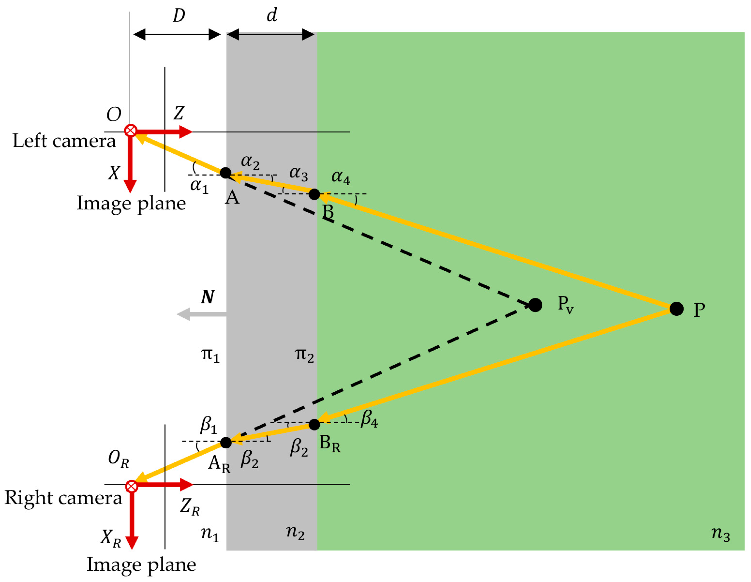
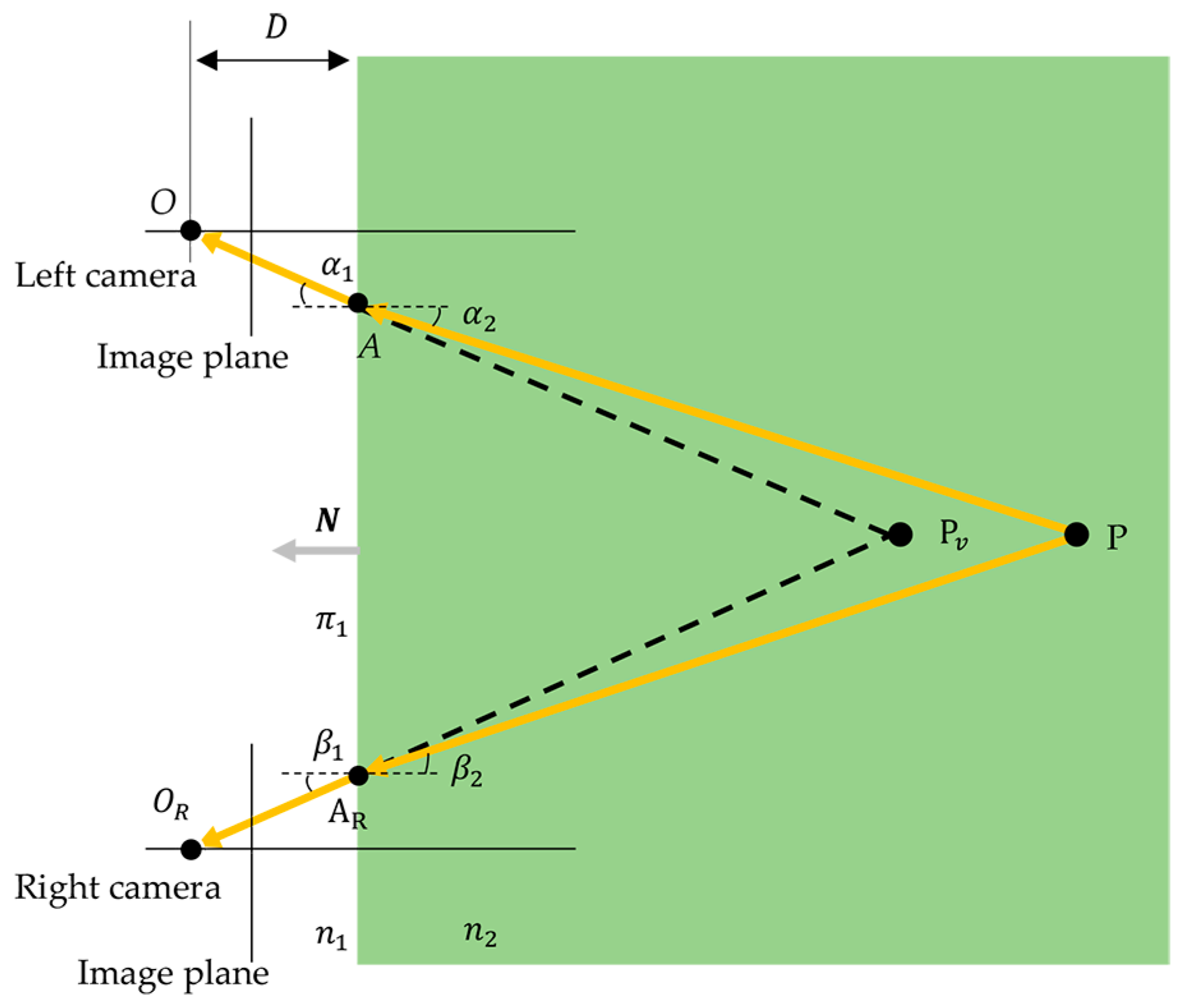
2.1. Measurement Model
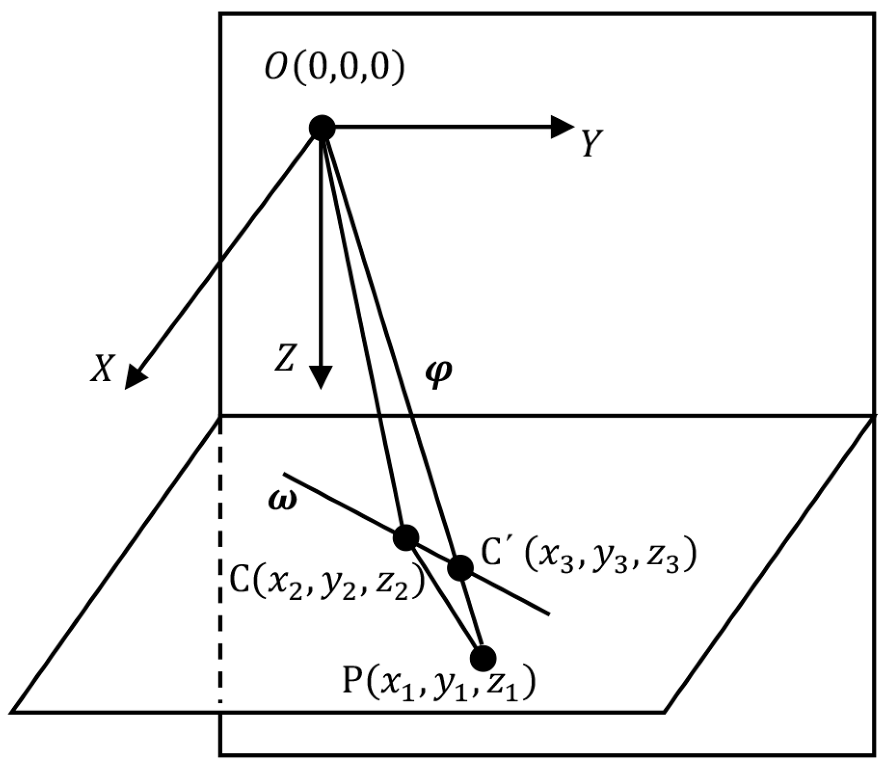
2.2. Dual-Medium Simulation Model
2.3. Simulation Experimental Design
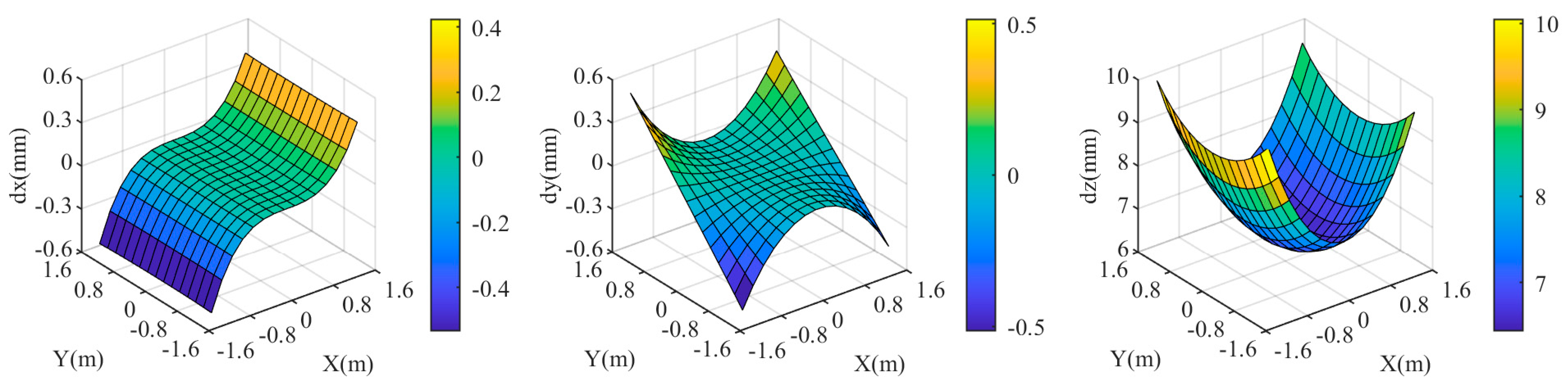
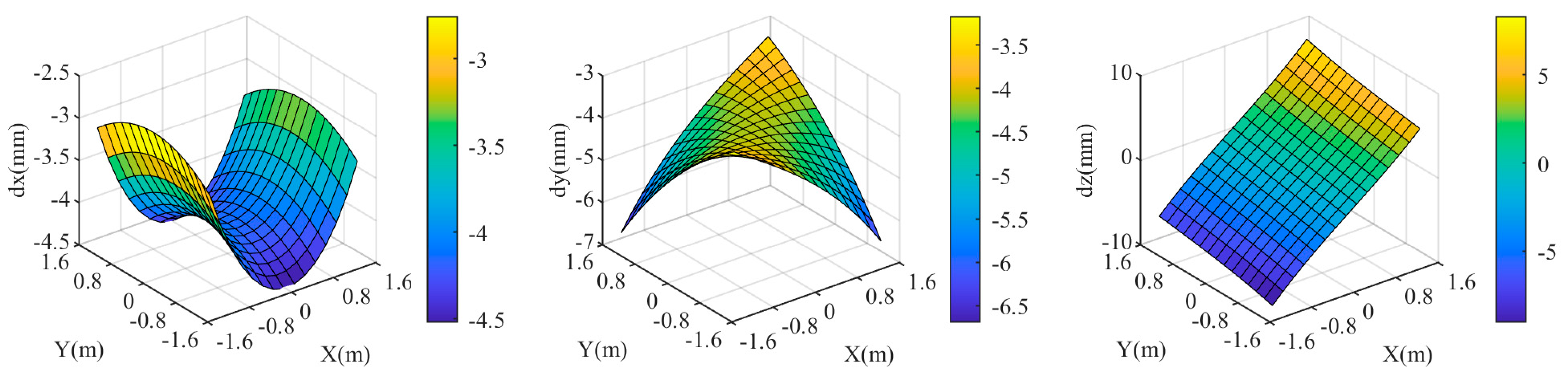
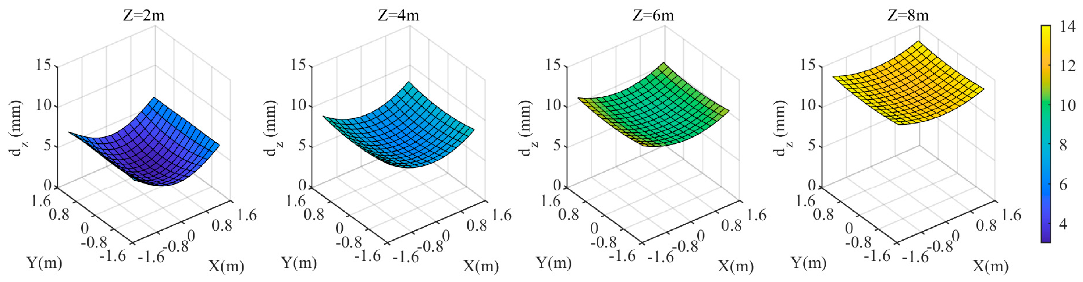
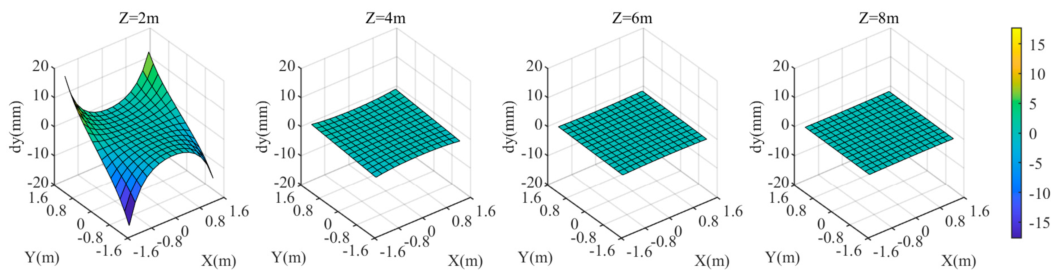
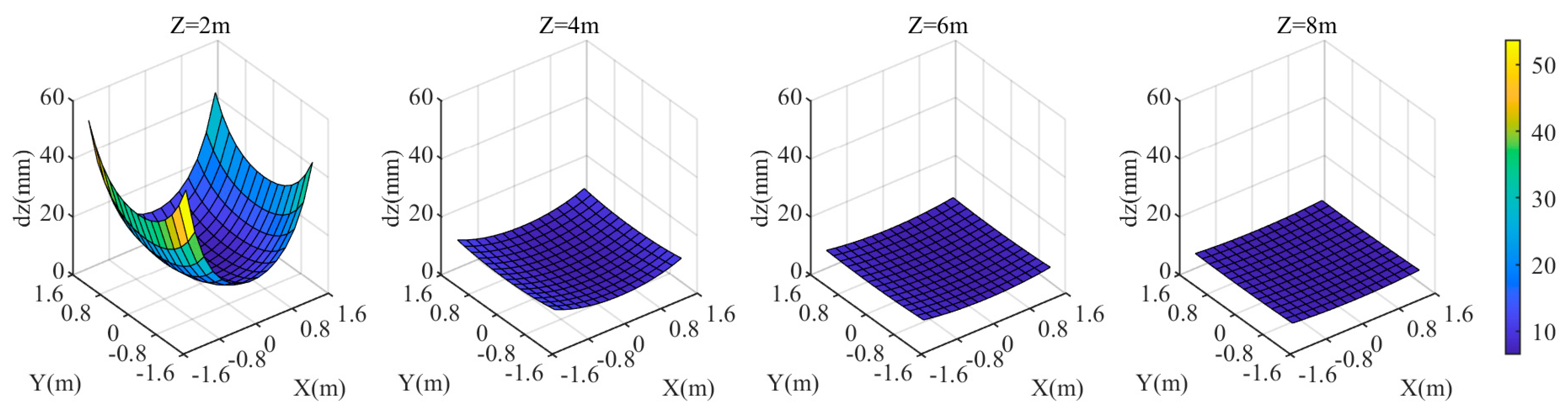
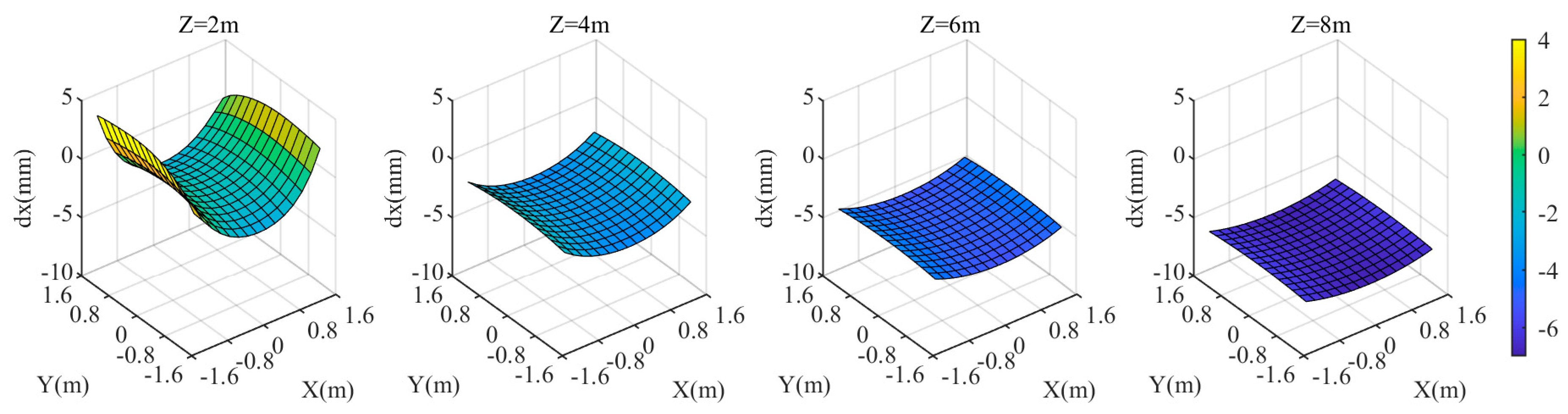
3. Results
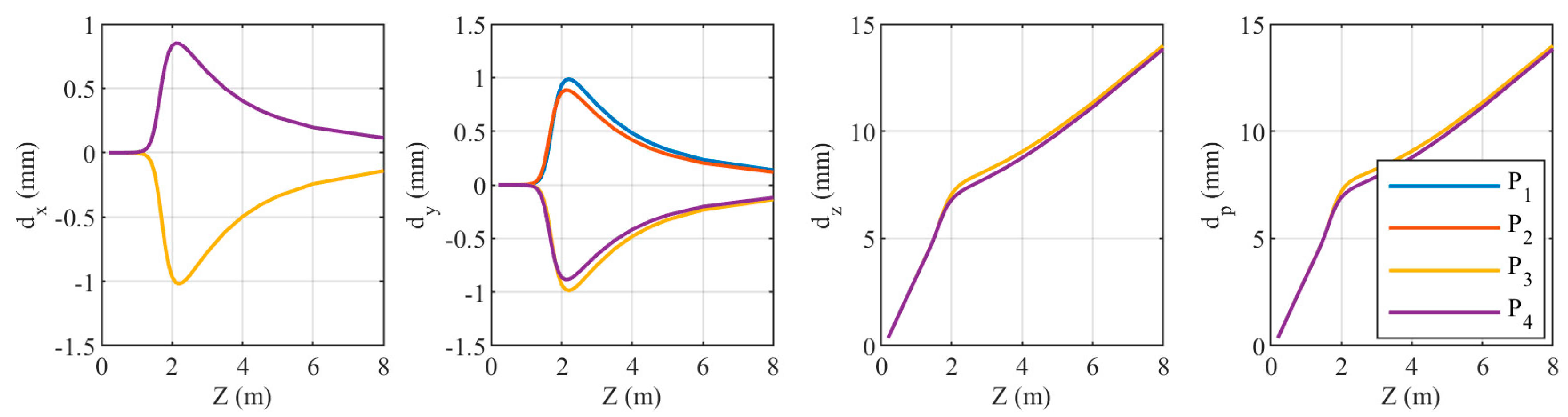
3.1. Experiment 1
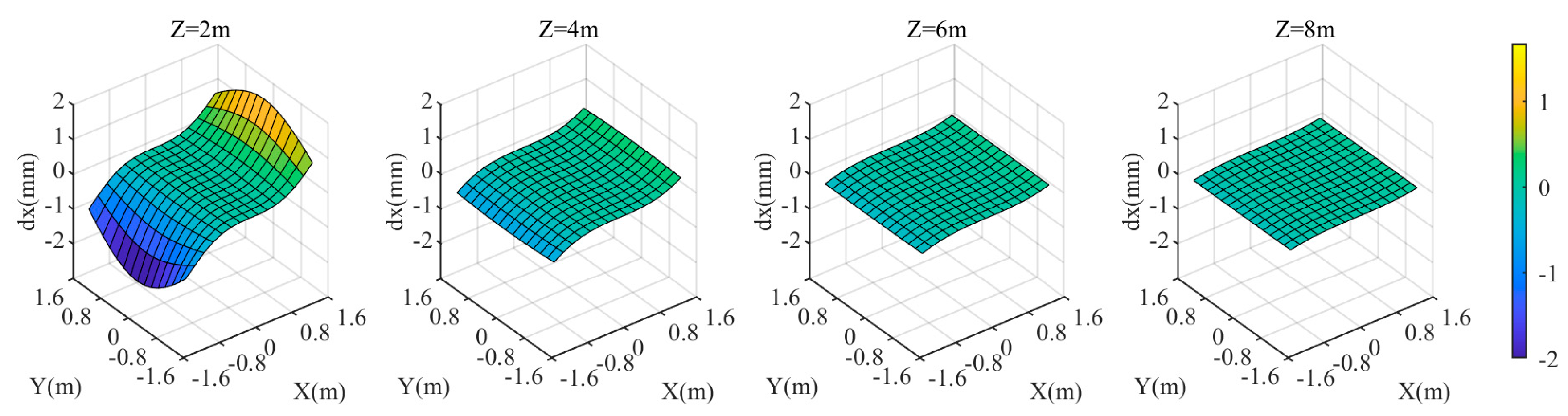
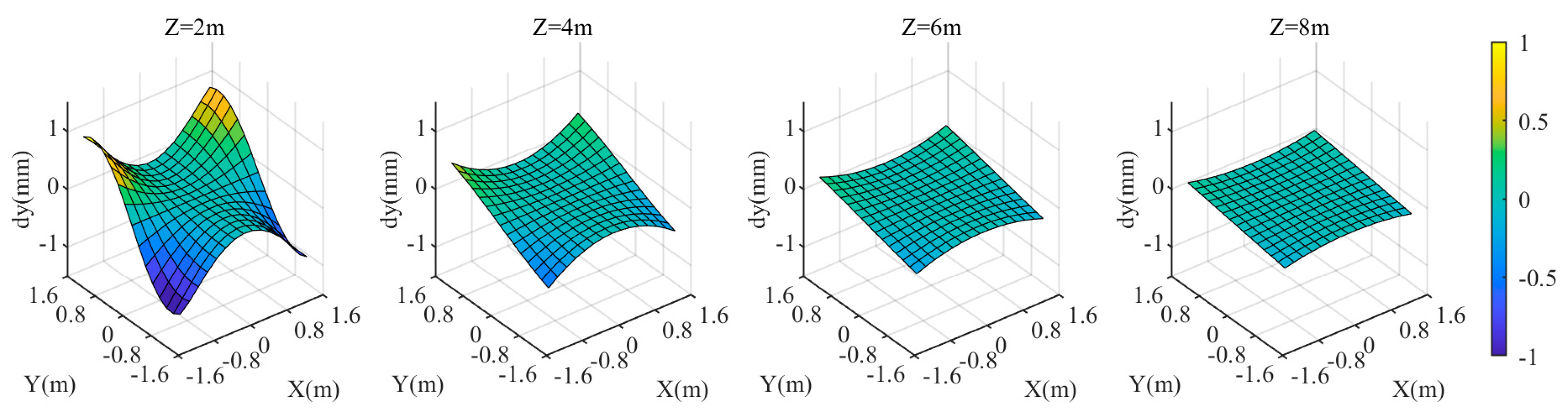
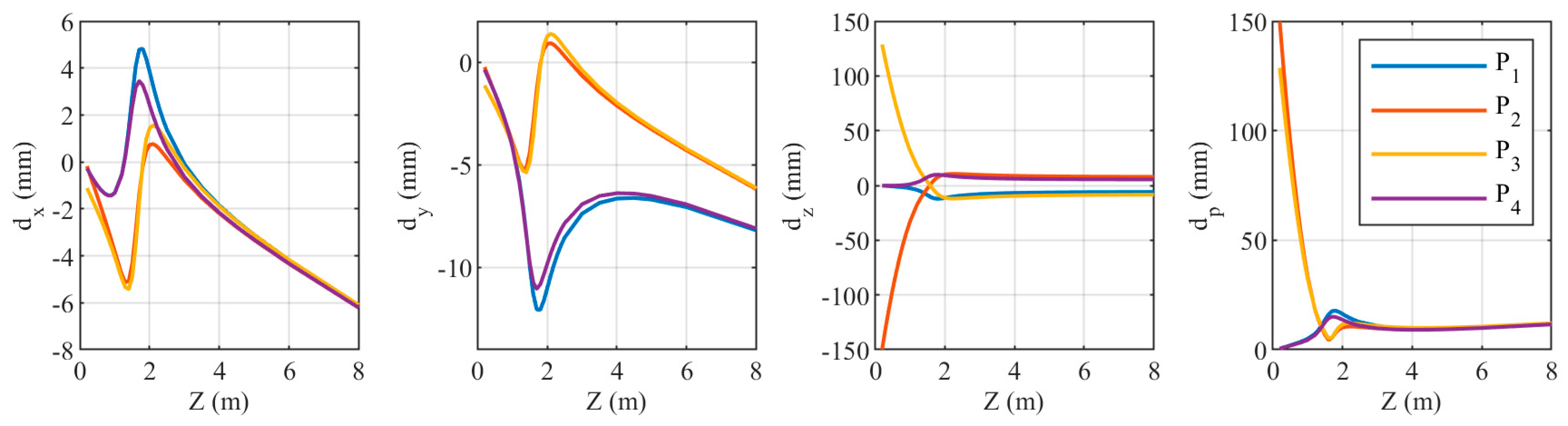
3.2. Experiment 2
3.2.1. Target Plane
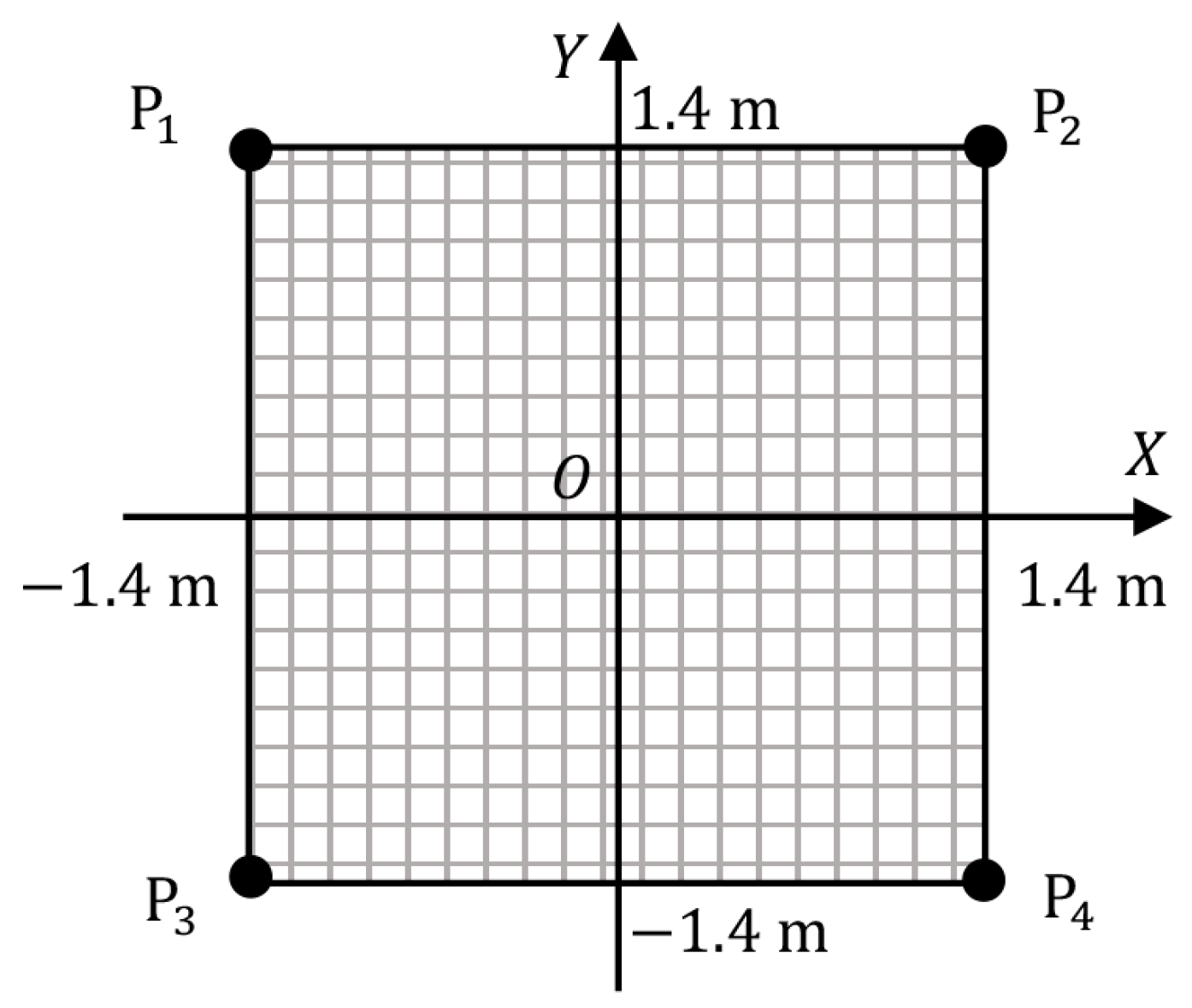
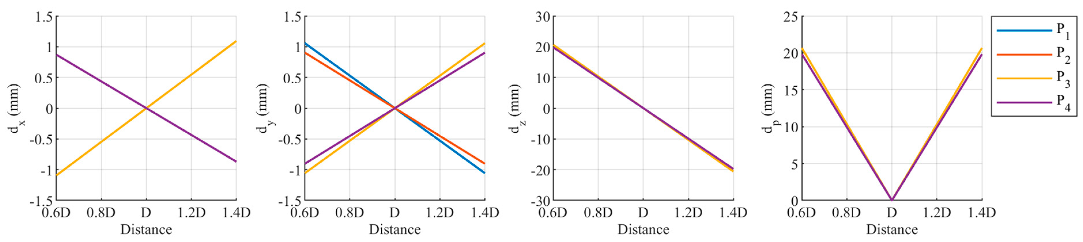
3.2.2. Fixed Points
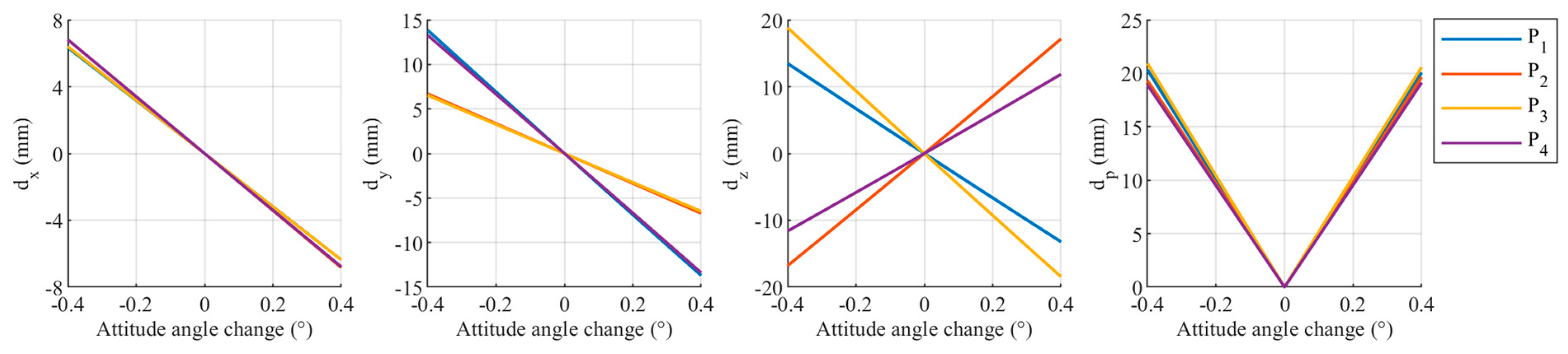
3.3. Experiment 3
4. Discussion
5. Conclusions
Author Contributions
Funding
Data Availability Statement
Conflicts of Interest
References
- Su, Z.; Pan, J.; Lu, L.; Dai, M.; He, X.; Zhang, D. Refractive three-dimensional reconstruction for underwater stereo digital image correlation. Opt. Express 2021, 29, 12131–12144. [Google Scholar] [CrossRef]
- Ding, T.; Sun, C.; Chen, J. Cross-medium imaging model and calibration method based on refractive optical path for underwater morphology measurement. Meas. Sci. Technol. 2024, 35, 15205. [Google Scholar] [CrossRef]
- Łuczyński, T.; Pfingsthorn, M.; Birk, A. The Pinax-model for accurate and efficient refraction correction of underwater cameras in flat-pane housings. Ocean. Eng. 2017, 133, 9–22. [Google Scholar] [CrossRef]
- Chi, Y.; Yu, L.; Pan, B. Low-cost, portable, robust and high-resolution single-camera stereo-DIC system and its application in high-temperature deformation measurements. Opt. Lasers Eng. 2018, 104, 141–148. [Google Scholar] [CrossRef]
- Wu, T.; Hou, S.; Sun, W.; Shi, J.; Yang, F.; Zhang, J.; Wu, G.; He, X. Visual measurement method for three-dimensional shape of underwater bridge piers considering multirefraction correction. Autom. Constr. 2023, 146, 104706. [Google Scholar] [CrossRef]
- Beall, C.; Lawrence, B.J.; Ila, V.; Dellaert, F. 3D reconstruction of underwater structures. In Proceedings of the 2010 IEEE/RSJ International Conference on Intelligent Robots and Systems IEEE, Taipei, Taiwan, 18–22 October 2010; pp. 4418–4423. [Google Scholar]
- Bruno, F.; Bianco, G.; Muzzupappa, M.; Barone, S.; Razionale, A.V. Experimentation of structured light and stereo vision for underwater 3D reconstruction. ISPRS J. Photogramm. Remote Sens. 2011, 66, 508–518. [Google Scholar] [CrossRef]
- Chadebecq, F.; Vasconcelos, F.; Lacher, R.; Maneas, E.; Desjardins, A.; Ourselin, S.; Vercauteren, T.; Stoyanov, D. Refractive Two-View Reconstruction for Underwater 3D Vision. Int. J. Comput. Vis. 2020, 128, 1101–1117. [Google Scholar] [CrossRef]
- Li, G.; Klingbeil, L.; Zimmermann, F.; Huang, S.; Kuhlmann, H. An Integrated Positioning and Attitude Determination System for Immersed Tunnel Elements: A Simulation Study. Sensors 2020, 20, 7296. [Google Scholar] [CrossRef] [PubMed]
- Liu, S.; Xu, H.; Lin, Y.; Gao, L. Visual Navigation for Recovering an AUV by Another AUV in Shallow Water. Sensors 2019, 19, 1889. [Google Scholar] [CrossRef] [PubMed]
- Cowen, S.; Briest, S.; Dombrowski, J. Underwater docking of autonomous undersea vehicles using optical terminal guidance. In Proceedings of the Oceans ’97. MTS/IEEE Conference, Halifax, NS, Canada, 6–9 October 1997; Volume 2, pp. 1143–1147. [Google Scholar]
- Liu, S.; Ozay, M.; Okatani, T.; Xu, H.; Sun, K.; Lin, Y. Detection and Pose Estimation for Short-Range Vision-Based Underwater Docking. IEEE Access 2019, 7, 2720–2749. [Google Scholar] [CrossRef]
- Treibitz, T.; Schechner, Y.; Kunz, C.; Singh, H. Flat Refractive Geometry. IEEE Trans. Pattern Anal. Mach. Intell. 2012, 34, 51–65. [Google Scholar] [CrossRef]
- Treibitz, T.; Schechner, Y.Y. Active Polarization Descattering. IEEE Trans. Pattern Anal. Mach. Intell. 2009, 31, 385–399. [Google Scholar] [CrossRef] [PubMed]
- Schechner, Y.Y.; Karpel, N. Recovery of Underwater Visibility and Structure by Polarization Analysis. IEEE J. Ocean. Eng. 2005, 30, 570–587. [Google Scholar] [CrossRef]
- Yamashita, A.; Kawanishi, R.; Koketsu, T.; Kaneko, T.; Asama, H. Underwater sensing with omni-directional stereo camera. In Proceedings of the 2011 IEEE International Conference on Computer Vision Workshops (ICCV Workshops), Barcelona, Spain, 6–13 November 2011; pp. 304–311. [Google Scholar]
- Menna, F.; Nocerino, E.; Fassi, F.; Remondino, F. Geometric and Optic Characterization of a Hemispherical Dome Port for Underwater Photogrammetry. Sensors 2016, 16, 48. [Google Scholar] [CrossRef] [PubMed]
- She, M.; Nakath, D.; Song, Y.; Köser, K. Refractive geometry for underwater domes. ISPRS J. Photogramm. Remote Sens. 2022, 183, 525–540. [Google Scholar] [CrossRef]
- Bosch, J.; Gracias, N.; Ridao, P.; Ribas, D. Omnidirectional Underwater Camera Design and Calibration. Sensors 2015, 15, 6033–6065. [Google Scholar] [CrossRef]
- Shmutter, B. Orientation Problems in Two-Medium Photogrammetry. Photogramm. Eng. 1967, 33, 1421–1428. [Google Scholar]
- Rinner, K. Problems of Two-Medium Photogrammetry. Photogramm. Eng. 1969, 35, 275–282. [Google Scholar]
- Masry, S.E.; Konecny, G. New Programs for the Analytical Plotter. Photogramm. Eng. 1970, 36, 1269–1276. [Google Scholar]
- Kwon, Y.; Casebolt, J.B. Effects of light refraction on the accuracy of camera calibration and reconstruction in underwater motion analysis. Sports Biomech. 2006, 5, 95–120. [Google Scholar] [CrossRef]
- Fabio, M.; Erica, N.; Salvatore, T.; Fabio, R. A photogrammetric approach to survey floating and semi-submerged objects. In Proceedings of the Videometrics, Range Imaging, and Applications XII, and Automated Visual Inspection, Munich, Germany, 13–16 May 2013. [Google Scholar]
- Kang, L.; Wu, L.; Yang, Y. Experimental study of the influence of refraction on underwater three-dimensional reconstruction using the SVP camera model. Appl. Opt. 2012, 51, 7591–7603. [Google Scholar] [CrossRef] [PubMed]
- Lavest, J.M.; Rives, G.; Laprest, J.T. Dry camera calibration for underwater applications. Mach. Vision. Appl. 2003, 13, 245–253. [Google Scholar] [CrossRef]
- Kang, L.; Wu, L.; Wei, Y.; Lao, S.; Yang, Y. Two-view underwater 3D reconstruction for cameras with unknown poses under flat refractive interfaces. Pattern Recognit. 2017, 69, 251–269. [Google Scholar] [CrossRef]
- Agrawal, A.; Ramalingam, S.; Taguchi, Y.; Chari, V. A theory of multi-layer flat refractive geometry. In Proceedings of the IEEE Conference on Computer Vision and Pattern Recognition (CVPR), Providence, RI, USA, 16–21 June 2012. [Google Scholar]
- Li, R.; Li, H.; Zou, W.; Smith, R.G.; Curran, T.A. Quantitative photogrammetric analysis of digital underwater video imagery. IEEE J. Ocean. Eng. 1997, 22, 364–375. [Google Scholar] [CrossRef]
- Jordt-Sedlazeck, A.; Koch, R. Refractive Structure-from-Motion on Underwater Images. In Proceedings of the IEEE International Conference on Computer Vision (ICCV), Sydney, NSW, Australia, 1–8 December 2013. [Google Scholar]
- Yau, T.; Gong, M.; Yang, Y. Underwater Camera Calibration Using Wavelength Triangulation. In Proceedings of the IEEE Conference on Computer Vision and Pattern Recognition (CVPR), Portland, OR, USA, 23–28 June 2013. [Google Scholar]
- Telem, G.; Filin, S. Photogrammetric modeling of underwater environments. ISPRS J. Photogramm. Remote Sens. 2010, 65, 433–444. [Google Scholar] [CrossRef]
- Chen, X.; Yang, Y.H. Two-View Camera Housing Parameters Calibration for Multi-layer Flat Refractive Interface. In Proceedings of the 2014 IEEE Conference on Computer Vision and Pattern Recognition, Columbus, OH, USA, 23–28 June 2014. [Google Scholar]
- Dolereit, T.; von Lukas, U.F.; Kuijper, A. Underwater stereo calibration utilizing virtual object points. In Proceedings of the Oceans 2015, Genova, Italy, 18–21 May 2015. [Google Scholar]
- Qiu, C.; Wu, Z.; Kong, S.; Yu, J. An Underwater Micro Cable-Driven Pan-Tilt Binocular Vision System with Spherical Refraction Calibration. IEEE Trans. Instrum. Meas. 2021, 70, 1–13. [Google Scholar] [CrossRef]
- Qi, G.; Shi, Z.; Hu, Y.; Fan, H.; Dong, J. Refraction calibration of housing parameters for a flat-port underwater camera. Opt. Eng. 2022, 61, 104105. [Google Scholar] [CrossRef]
- Ma, Y.; Zhou, Y.; Wang, C.; Wu, Y.; Zou, Y.; Zhang, S. Calibration of an underwater binocular vision system based on the refraction model. Appl. Opt. 2022, 61, 1675–1686. [Google Scholar] [CrossRef]
- Tong, Z.; Gu, L.; Shao, X. Refraction error analysis in stereo vision for system parameters optimization. Measurement 2023, 222, 113650. [Google Scholar] [CrossRef]


| D | N | |
|---|---|---|
| 10 cm |
Disclaimer/Publisher’s Note: The statements, opinions and data contained in all publications are solely those of the individual author(s) and contributor(s) and not of MDPI and/or the editor(s). MDPI and/or the editor(s) disclaim responsibility for any injury to people or property resulting from any ideas, methods, instructions or products referred to in the content. |
© 2024 by the authors. Licensee MDPI, Basel, Switzerland. This article is an open access article distributed under the terms and conditions of the Creative Commons Attribution (CC BY) license (https://creativecommons.org/licenses/by/4.0/).
Share and Cite
Li, G.; Huang, S.; Yin, Z.; Zheng, N.; Zhang, K. Analysis of the Influence of Refraction-Parameter Deviation on Underwater Stereo-Vision Measurement with Flat Refraction Interface. Remote Sens. 2024, 16, 3286. https://doi.org/10.3390/rs16173286
Li G, Huang S, Yin Z, Zheng N, Zhang K. Analysis of the Influence of Refraction-Parameter Deviation on Underwater Stereo-Vision Measurement with Flat Refraction Interface. Remote Sensing. 2024; 16(17):3286. https://doi.org/10.3390/rs16173286
Chicago/Turabian StyleLi, Guanqing, Shengxiang Huang, Zhi Yin, Nanshan Zheng, and Kefei Zhang. 2024. "Analysis of the Influence of Refraction-Parameter Deviation on Underwater Stereo-Vision Measurement with Flat Refraction Interface" Remote Sensing 16, no. 17: 3286. https://doi.org/10.3390/rs16173286
APA StyleLi, G., Huang, S., Yin, Z., Zheng, N., & Zhang, K. (2024). Analysis of the Influence of Refraction-Parameter Deviation on Underwater Stereo-Vision Measurement with Flat Refraction Interface. Remote Sensing, 16(17), 3286. https://doi.org/10.3390/rs16173286