Abstract
In the realm of precision space applications, improving the accuracy of orbit determination (OD) is a crucial and demanding task, primarily because of the presence of measurement noise. To address this issue, a novel machine learning method based on bidirectional long short-term memory (BiLSTM) is proposed in this research. In particular, the proposed method aims to improve the OD accuracy of Earth–Moon Libration orbits with angle-only measurements. The proposed BiLSTM network is designed to detect inaccurate measurements during an OD process, which is achieved by incorporating the least square method (LSM) as a basic estimation approach. The structure, inputs, and outputs of the modified BiLSTM network are meticulously crafted for the detection of inaccurate measurements. Following the detection of inaccurate measurements, a compensating strategy is devised to modify these detection results and thereby reduce their negative impact on OD accuracy. The modified measurements are then used to obtain a more accurate OD solution. The proposed method is applied to solve the OD problem of a 4:1 synodic resonant near-rectilinear halo orbit around the Earth–Moon L2 point. The training results reveal that the bidirectional network structure outperforms the regular unidirectional structures in terms of detection accuracy. Numerical simulations show that the proposed method can reduce the estimated error by approximately 10%. The proposed method holds significant potential for future missions in cislunar space.
1. Introduction
The interest in space exploration and the development of space techniques have led to a rapid increase in the number of spacecraft [,,,]. As a result, the need for accurate orbit determination (OD) has become even more crucial for managing long-term space operations [,,,]. OD provides valuable state information that aids in subsequent orbit uncertainty propagation [,,,], guidance [,,], and control [,,]. Currently, there are two main groups of state-of-the-art approaches for OD: the Kalman filter (KF) and its variants and the least square method (LSM) and its variants [,,,,]. These methods can obtain optimal estimations by combining the state propagation and incoming measurements.
The OD task can be challenging, especially when dealing with short-arc, sparse, and noisy measurements, as well as highly nonlinear dynamics environments [,,]. To improve the accuracy of OD, various methods have been developed. These methods include the extended Kalman filter (EKF) [], the unscented Kalman filter (UKF) [,], the cubature Kalman filter (CKF) [,,], and the conjugate unscented Kalman filter (CUKF) [,], all based on the KF algorithm. These methods can capture higher-order terms of the state and measurement equations, which leads to more accurate estimations. However, they also introduce more computational complexity [,,].
The field of space and astrodynamics is witnessing a surge in interest in machine learning approaches, owing to the rapid development of artificial intelligence [,,]. These approaches provide a promising alternative to enhance the accuracy of orbit prediction and estimation [,,]. Peng and Bai first proposed an ML-based framework to improve orbit prediction accuracy, in which a support vector machine (SVM) [] is embedded into a physical-based model to compensate for orbit prediction errors due to the lack of explicit dynamics models. Apart from the SVM, Peng and Bai investigated the artificial neural network (ANN) [] and Gaussian processes (GPs) [] for the same purpose, and a comprehensive comparison of these three ML approaches is provided in []. Additionally, they proposed a fusion strategy to integrate the ML model with conventional OD methods such as the EKF []. These methods are validated to be effective and efficient in simulation-based environments and publicly available data []. In addition to the work of Peng and Bai, the boosting tree (BT) and long short-term memory (LSTM) network have also been employed to model the underlying pattern of orbit estimation. Li et al. employed a BT-based method to model the underlying pattern from past OD data and improve the current OD accuracy of space debris under sparse measurements []. Zhou et al. proposed a hybrid method for the OD of a continuously maneuvering spacecraft, in which an LSTM network is used to detect and compensate for the maneuver [,]. Zhou et al. further proposed a deep neural network (DNN)-based method to compensate for the errors of the low-fidelity dynamics to improve OD accuracy [].
The proposed method for improving OD accuracy does not rely on modeling the underlying patterns of dynamics like other ML-based approaches. Instead, it focuses on detecting and compensating for inaccuracies in measurements, using a modified bidirectional long short-term memory (BiLSTM) network fused with an LSM. The training data were carefully designed with a focus on input and output structures, with measurements identified as inaccurate if their error is greater than two times the standard deviation (STD). The modified BiLSTM network was then trained to predict which measurements belong to this inaccurate class. One of the advantages of using a BiLSTM network structure is that it can address sequential inputs, making it more adaptable and better at generalizing. Furthermore, the bidirectional structure allows for the use of both past and future information to detect inaccurate measurements at the current epoch, which is not possible with conventional unidirectional LSTM networks. To correct these inaccuracies, a compensation strategy is proposed, and the LSM is used to estimate the orbit. This method is then applied to solve the OD problem of a 4:1 synodic resonant near-rectilinear halo orbit (NRHO) in the Earth–Moon three-body system with promising results.
The remainder of this paper is organized as follows. The essential background and mathematical formulations are given in Section 2. The methodology of the proposed BiLSTM-based machine learning approach to improve OD accuracy is presented in Section 3. Numerical simulations are performed in Section 4, and the conclusions are given in Section 5.
2. Preliminaries
2.1. Least Square Method
First, consider an OD system with a state equation and a measurement equation as follows [,]:
where is the state vector of the spacecraft; and represent the position and velocity vectors, respectively; is the dynamics model of the spacecraft; and denote the measurement vector and the measurement model, respectively; is Gaussian-distributed measurement noise; and m is the dimension of the measurement.
Let be the initial estimated state of the spacecraft at the initial epoch , which can be obtained from an initial OD process or orbit propagation based on a previous OD solution. Then, the estimated orbit at any specified epoch t can be computed by propagating using the dynamics . Let and be the deviations of the initial estimated state and the estimated state , respectively. A first-order mapping relationship from to is given by
where represents the state transform matrix (STM). The STM can be obtained by integrating along the estimated orbit .
Let represent the predicted measurement of the estimated state . By performing a Taylor series expansion of the measurement model in terms of the estimated state , the relationship between the deviation of the predicted measurement and the deviation of the estimated state can be approximated as
where .
Assume that n measurements () are available, at known epochs , where is the measurement noise. The residual between the true measurement and the predicted measurement can be written as
The goal of the LSM is to obtain an optimal estimation that minimizes the residual between the true and predicted measurements []. Therefore, the performance metric is written as
The optimal estimation can be computed by solving the equation given by
and the initial estimated state is renewed as .
Notice that the optimal estimation from Equation (10) is not sufficiently accurate, as only the linear terms are considered during the derivation process (i.e., Equations (2) and (3)). Thus, iterations are needed to make the estimation converge to a specified accuracy. The pseudocode of the LSM is shown as Algorithm 1. The inputs of the algorithm are the dynamics and measurement models, income measurements, initial estimated state , maximal iteration , and threshold . When the Frobenius norm of the optimal estimation is smaller than the given threshold, i.e., , the LSM is considered converged. In this work, the threshold is set to .
| Algorithm 1: Pseudocode of least squares method [] |
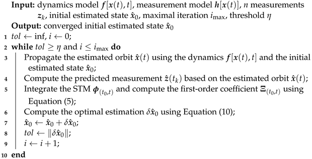 |
2.2. Networks For Addressing Sequential Inputs
The OD is essentially a sequential input problem, as a single incoming measurement is usually insufficient to determine the orbit state. In this subsection, three networks, i.e., the recurrent networks (RNN), LSTM and BiLSTM, that can address sequential inputs are introduced.
2.2.1. RNN
RNN is an elegant way to deal with (epoch) sequential inputs [,]. In contrast to conventional machine learning methods, such as SVM [], ANN [], GPs [], and BT [], which require a fixed number of inputs, the RNN architecture can make use of all the available input information up to the current epoch to predict the current label [,]. However, the standard RNN suffers from some drawbacks, such as gradient explosion and disappearance, and not retaining long-distance information [].
2.2.2. LSTM
The LSTM network is an improved network model extended from the RNN [,]. By adding a gating mechanism in the LSTM structure, the drawbacks of the RNN are solved to a certain extent. A standard LSTM structure is shown in Figure 1, in which , , and represent the input state, the hidden state, and the cell state of the k-th LSTM cell (corresponding to epoch ), respectively. The hidden state and the cell state are used to control and store the long-term information of the input state . At any specified epoch , the inputs of the k-th LSTM cell include the current input state , the previous hidden state and the previous cell state , whereas the outputs are the current hidden state and the current cell state . The mathematical model of the k-th LSTM cell is given as
where and are the weight and bias, respectively, (i.e., in Figure 1) and represent the sigmoid and tanh activation functions, respectively, and ⊗ denotes the elementwise vector multiplication.
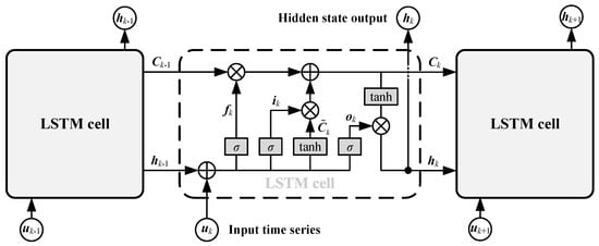
Figure 1.
Structure of a standard LSTM network.
2.2.3. BiLSTM
As presented in Figure 1, the outputs of the k-th LSTM cell (i.e., and ) depend on all the inputs up to the current epoch . However, future input information coming up later than the current epoch can also be useful for the current output prediction []. To make use of all available input information, including previous, current, and future inputs, the BiLSTM network is proposed, which uses two separate LSTM networks (one for each time direction) and then merges the results [,]. The structure of a standard BiLSTM network is shown in Figure 2. The BiLSTM network contains two independent LSTM layers, i.e., the forward and reverse LSTM layers, with each BilSTM cell consisting of two LSTM cells, i.e., a forward LSTM cell and a reverse LSTM cell. The input and output vectors of different LSTM cells in the BiLSTM network are detailed in Table 1.
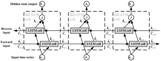
Figure 2.
Structure of a standard BiLSTM network.

Table 1.
Inputs and outputs of LSTM cells in the BiLSTM network.
All the hidden states from the LSTM layer are arranged in chronological order and in reverse order. Then, the forward hidden state sequence and its reverse sequence are obtained. The BiLSTM hidden state is computed using a connecting function , given by
3. Methodology
In this section, the methodology for improving OD accuracy using BiLSTM is provided. The proposed method improves OD accuracy by detecting inaccurate measurements and then compensating for those measurements. A modified BiLSTM neutral network is designed for inaccurate measurement detection. In this paper, the OD of a spacecraft near the Earth–Moon L2 point using angle-only measurements from a ground-based station is taken as an example to show the sample construction and training processes of the modified BiLSTM neutral network.
3.1. Dynamics and Measurement Model
The high-fidelity dynamics model of a spacecraft in cislunar includes the point-mass gravity field from the Earth, Moon, and Sun (using the ephemeris VSOP2000 [,,]), given as
where and are the position and velocity vector in Earth-centered equatorial inertial (ECI) coordinates, respectively; , and are gravitational constants of the Earth, the Sun, and the Moon, respectively; and and label the positions of the Sun and Moon in ECI coordinates respectively.
Assume that a ground-based station can measure the line-of-sight (LOS) direction from the station to the spacecraft. The LOS direction can be represented by two angles, i.e., the right ascension (RA) () and the declination (DEC) () [,,]. Therefore, the measurement model used in this work can be written as
where denotes the position vector of the station in the ECI coordinate at a specified epoch t. The standard deviation (STD) of the noises of RA and DEC are set to be , i.e., . The parameters of the ground-based station used in this work are shown in Table 2. The azimuth range restriction of the ground-based station is ignored, and only the elevation restriction is considered. The spacecraft is invisible when it is on the opposite side of Earth. Thus, the elevation should be constrained in deg.
Table 2.
Parameters of the ground-based station used.
3.2. Sample Construction
Careful design of the structure of the training sample is vital for the network to accurately detect inaccurate measurements. The construction of the sample dataset for the BiLSTM-based approach is illustrated in Figure 3. Figure 3a,b present the cases without and with inaccurate measurements, respectively. In Figure 3, the black solid and dashed curves denote the true orbit and the estimated orbit obtained from the LSM, respectively.
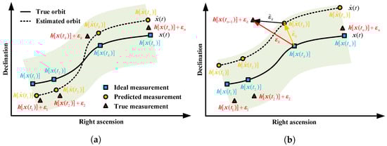
Figure 3.
Illustration of the sample dataset for the BiLSTM-based approach to improve OD accuracy. (a) Case without inaccurate measurements; (b) case with inaccurate measurements.
As annotated in Figure 3, three types of measurements, the ideal measurements , the true measurements and the predicted measurements , are represented by blue squares, red triangles and orange circles, respectively. The light green regions are admissible regions of measurements. In this work, the admissible regions are defined as the regions where the measurement noises are smaller than two times the STD. The measurements inside and outside the admissible regions are defined as accurate and inaccurate measurements, respectively. As shown in Figure 3a, the estimated orbit is close to the true orbit when the true measurements are located in the admissible region, while the estimated errors are large when some of the true measurements are outside the admissible region (see Figure 3b).
According to Figure 3, three types of measurement errors are defined at a specified epoch :
- True measurement error . Note that the true measurement error is equivalent to the measurement noise defined in Equation (1).
- Predicted measurement error .
- Relative measurement error .
The three types of measurement errors can be related using the following equation:
Among the three types of measurement errors mentioned above, the true measurement error can directly evaluate whether the true measurement is inside the admissible regions. Unfortunately, the true measurement error is unavailable, as one can never know the true state of a spacecraft. Only the relative measurement error is available during the OD process. The relative measurement error is related to the true measurement error , which is expected to carry the necessary information for detecting inaccurate measurements.
Next, the structure of the training sample is constructed. Apart from the relative measurement error , there are also some variables, such as the true measurements and predicted state, that are available and might contain useful information for inaccurate measurement detection. Taking a specified epoch as an instance, the learning variables of the sample dataset are given as follows:
- The relative measurement error . The relative measurement error is assumed to contain information related to the true measurement error .
- The variables related to the measurements, including the true measurements and the position of the ground-based station (in the ECI coordinate) . These variables may reflect the sensitivity of the estimated errors to measurement errors.
- The estimated state obtained using the LSM. The estimated state can reflect the physical information of the orbit, for example, the orientation and the distance of the spacecraft.
- The measurement interval (). When , in this work. The measurement interval is an important variable, as the longer the measurement interval is, the weaker the relationship between two successive measurements.
With the aforementioned learning variables, the input vector of the sample dataset at a specified epoch is written as
Inaccurate measurement detection is essentially a binary classification problem. Motivated by [], the output vector of the sample dataset at epoch is expressed as
where , , and . and mean that RA is inside and outside the admissible region, respectively, whereas and mean that DEC is inside and outside the admissible region, respectively. This type of output form is particularly common in binary classification problems. In this way, the cross entropy can be used as a loss function to train the network.
Note that the output at the current epoch is related not only to the current input , but also to the inputs at the previous and future epochs. By collecting all the inputs () and sequentially processing them, the output can be better predicted. Thus, the structure of the sample dataset is written as
where denotes the sample dataset, and and are the input and output sets of the sample dataset , respectively. Note that the number of inputs and outputs in one sample , n, is not fixed in our work, as the number of incoming measurements in an OD process is arbitrary.
Based on the above discussion on sample input and output, a method is proposed for effectively generating a large number of samples herein. First, three groups of Earth–Moon LPOs, i.e., a group of Southern L2 Halo orbits, a group of Northern L2 Halo orbits, and a group of L2 Lyapunov orbits, are generated []. The nondimensional orbits in the circle restrict three-body problem (CRTBP) are shown in Figure 4. The corresponding nondimensional initial conditions, periods, and Jacobi constants of the Southern L2 Halo and L2 Lyapunov orbits are listed in Table 3 and Table 4, respectively, where T and J denote the orbit period and Jacobi constant, respectively. The Northern L2 Halo family can be obtained by reflecting the southern Halo family across the x-y plane.
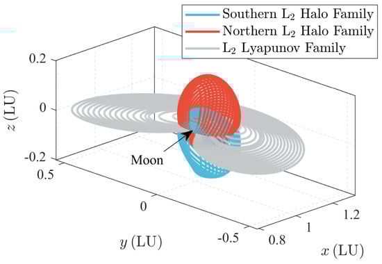
Figure 4.
An illustration of orbit families for sample generation.
Table 3.
Orbit parameters of the Southern L2 Halo family [,].
Table 4.
Orbit parameters of the Lyapunov family [,].
Moreover, the nondimensional Southern L2 Halo and L2 Lyapunov orbits in the Earth–Moon CRTBP are plotted in Figure 5a and Figure 5b, respectively, with the colors representing the Jacobi constant of the orbits. According to Table 3 and Table 4, 25 Southern L2 Halo orbits, 25 Northern L2 Halo orbits, and 21 L2 Lyapunov orbits are obtained. Notice that the second L2 Lyapunov orbit repeatedly appears in the southern and Northern L2 Halo families. Therefore, 69 nondimensional periodic orbits are available after the repetitive orbits are removed.
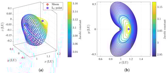
Figure 5.
Earth–Moon Libration point orbits in the nondimensional rotating coordinate. (a) Earth–Moon L2 Halo orbits; (b) Earth–Moon L2 Lyapunov orbits.
Second, these nondimensional periodic orbits are corrected in the high-fidelity ephemeris force model (i.e., Equation (13)) using the two-level differential corrector [], after which 69 ephemeris trajectories are computed. These ephemeris trajectories are propagated using the Runge–Kutta (4,5) solver [] with a relative tolerance of 10−12 and an absolute tolerance of 10−12, with an initial epoch of 1 Jan 2020 and a propagation period of 1 month (approximately 27.32 days). The ephemeris trajectories of the 25th Halo orbit and 21st Lyapunov orbit are presented in Figure 6a and Figure 6b, respectively.
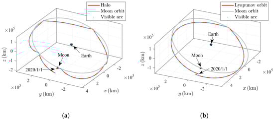
Figure 6.
Earth–Moon Libration point orbits in the ECI coordinate. (a) The 25th Earth–Moon L2 Halo orbit; (b) The 21st Earth–Moon L2 Lyapunov orbit.
Next, each ephemeris trajectory is discretized into several points, with a constant interval of 6 h. In this way, 7590 points are obtained. For each point, one sample is constructed using the following steps:
Step 1: The state and associated epoch of the point are taken as the initial state and epoch of one OD, i.e., and . The time of flight (i.e., the measurement duration) , the number of measurements n, and the initial estimated error are randomly generated based on the lower and upper bounds listed in Table 5. The final epoch is calculated as . The first and final measurements are assumed to be available at the initial and epochs, i.e., and . The epochs of the remaining measurements, () are randomly generated using the Latin hypercube sampling method [] over the duration .
Table 5.
Parameter ranges for generating samples.
Step 2: Propagate the true orbit using the high-fidelity ephemeris force model in the duration . Check the visibility over the duration according to the feasible elevation range in Table 2. If visible, go to Step 3.
Step 3: Calculate the ideal measurement at n epochs (). Randomly generate the true measurement error according to the given STDs (i.e., ). Compute the true measurement . Check whether the true measurement error exceeds the admissible region. If the true measurement error of RA is inside the admissible region, and , whereas if the true measurement error of RA is outside the admissible region, and , which are the same for DEC. Then, the output set is obtained.
Step 4: The initial estimated state is obtained using . Compute the optimal estimated state using the LSM. The input set is then constructed using Equations (16) and (17).
Step 5: A sample is constructed as .
Using the above process, 3761 valid samples are obtained. All these samples, including the inputs and outputs, are normalized to . Notice that in the ECI coordinate is a constant. Thus, in this work, is normalized to 0.5. In the following subsections, the modified BiLSTM network is trained using these samples.
3.3. Modified BiLSTM Structure
With the sample from Equation (18) given, the structure of the designed modified BiLSTM network is displayed in Figure 7. Apart from n BiLSTM cells, the modified BiLSTM network also contains two initialization layers, a pre-BiLSTM layer, a post-BiLSTM layer, and a sigmoid layer.
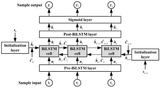
Figure 7.
Structure of the designed modified BiLSTM network.
As shown in Figure 7, the pre-BiLSTM layer is applied to the first layer of the designed network, which is employed to extract the useful features from the sequential input (as defined in Equation (16)). The BiLSTM cells serve as the second layer, which is expected to fully learn information extracted by the pre-BiLSTM layer. The forward and backward association characteristics of the relative measurement errors, true measurements, station positions, estimated states, and measurement intervals of different epochs are abstracted and merged by the BiLSTM cells. Then, using a post-BilSTM layer, the hidden states obtained from the BiLSTM cells are reweighted. In this way, the key features will be given more weight to reduce interferences from inconsequential information and improve the classification performance. The sigmoid layer is the last layer in the designed network, which is a typical operation in binary classifications. The sigmoid function is a mathematical function that takes any real number and “squashes” it into a range between 0 and 1. It is often used in machine learning and neural networks to introduce non-linearity and convert an input into a probability [,]. The function has an S-shaped curve and is expressed as . This function is particularly useful for scenarios where we need to make predictions or classify data into two categories. Its smooth gradient also makes it useful for efficient learning during backpropagation in neural networks. In addition, two initialization layers are added to the network to generate the hidden states and . The input vectors of two initialization layers, and , are assumed to be 14-dimensional zero vectors, i.e., .
The initialization, pre-BiLSTM, post-BiLSTM, and sigmoid layers are designed as deep neural networks (DNNs). A standard DNN contains input, output, and hidden layers [], with its structure presented in Figure 8. In Figure 8, each circle represents a neuron. The sigmoid layer is designed as a three-layer fully connected DNN with the sigmoid as the activation function. The initialization, pre-BiLSTM and post-BiLSTM layers are assumed to have the same structure in their hidden layers, i.e., the number of hidden layers, the number of neurons and the activation function used are the same. Let L and M denote the number of hidden layers and the corresponding number of neurons in one hidden layer, respectively. Moreover, the dimensions of the hidden and cell states of the BiLSTM cells are also set to M, and and are assumed to be M-dimensional zero vectors. According to the above discussion, the structures of the four layers are shown in Table 6. Notice that in this work, two independent networks are trained for anomaly detection of RA and DEC; therefore, the dimension of the predictions of the proposed modified BiLSTM network is 2.
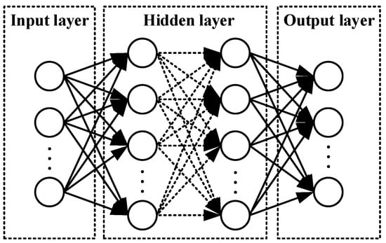
Figure 8.
Structure of a standard DNN network.
Table 6.
Structures of the initialization, pre-BiLSTM, post-BiLSTM, and sigmoid layers.
3.4. Training Process and Results
Before training the modified BiLSTM network, the 3761 samples are randomly divided into two sample datasets: one training dataset and one validation dataset. The training dataset contains 80% of the samples (3009 samples), and the validation dataset has the remaining 20% (662 samples). The training dataset is used to train the modified BiLSTM network, whereas the validation dataset is used to test its accuracy. In this paper, the modified BiLSTM networks for inaccurate RA and DEC detection are called RA BiLSTM and DEC BiLSTM, respectively. In this work, the construction and training of the modified BiLSTM network are based on the Python implementation of PyTorch. The cross-entropy loss is employed as the loss function during the training process. For RA, the cross-entropy loss of one sample is written as
whereas for DEC, the cross-entropy loss of one sample is given as
where and are the predictions of the RA BiLSTM and DEC BiLSTM, respectively.
In addition, the maximal iteration is set to 100. In each iteration, the 3009 samples from the training dataset are sequentially trained. The parameters of the modified BiLSTM networks are updated once one sample is trained. Thus, the parameters are updated 3009 times in one iteration. The learning rate is initialized as and decayed by 0.98 every iteration, given as
where lr and iter denote the learning rate and the number of iterations, respectively.
In each iteration, the cross-entropy loss of 3009 training samples and 662 validation samples are recorded. The mean cross-entropy (MCE) losses of the training and validation datasets are then calculated. The network parameters with minimal validation MCE are retained and used in the subsequent inaccurate measurement detection. It takes approximately 2 h to train the neural network using a workstation (CPU: 13th Gen Intel(R) Core(TM) i9-13900KF; GPU: NVIDIA GeForce RTX 4090). The training results of the modified BiLSTM networks with different structures are listed in Table 7. Several conclusions can be drawn from Table 7. First, for the concerned anomaly detection problem, the network with one hidden layer performs better than that with two hidden layers. Second, the minimal validation MCEs using Leaky ReLU are smaller than those using ReLU and Tanh. Third, the networks with 32 neurons per layer are more accurate than those with 16, 64, and 128 neurons per layer. Therefore, the modified BiLSTM network with one hidden layer, thirty-two neurons in the hidden layer, and the Leaky ReLU activation function is chosen to detect inaccurate measurements in this work.
Table 7.
Training results of networks with different structures.
The time histories of the MCE of the chosen network are plotted in Figure 9. It can be seen from Figure 9 that the training and validation MCEs decrease synchronously as the iteration increases. The modified BiLSTM networks have not overfitted during the training process, meaning that the design of the inputs, outputs, and structure of the networks is reasonable.
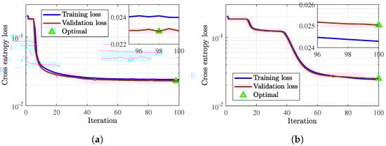
Figure 9.
Training convergence history. The green triangle represents the iteration of the minimal validation MCE. (a) RA, (b) DEC.
To verify the classification accuracy of the trained network, 3629 new samples that are different from the previously obtained 3761 samples are randomly generated using the same method in Section 3.2. The trained networks are employed to detect inaccurate measurements for each newly generated sample. The accuracy rate (AR) is employed as the metric to evaluate the performance of the networks, which is defined as the percentage of all the measurements belonging to each class that are correctly classified. Taking a specified sample with n inputs and n outputs as an example, the AR of the inaccurate class is defined as
where and () represent the number of inaccurate measurements and the number of inaccurate measurements that are correctly classified, respectively.
The ARs of 3629 newly generated samples are computed and shown in Figure 10. Scatter plots are provided in the left subplots of Figure 10a,b, in which the x- and y-axes represent the number of measurements and the AR, respectively. Additionally, violin plots are provided in the right subplots of Figure 10a,b. The violin plot depicts distributions of the corresponding ARs using density curves. The width of each curve corresponds with the approximate frequency of the ARs in each region. In the middle of each density curve is a small box plot, with the rectangle showing the ends of the first and third quartiles and the central showing the median. It can be seen from Figure 10 that the ARs of the accurate class are higher than 95%. For most samples, the ARs of the inaccurate class are higher than 80%. In addition, the predicted accuracy is better as the number of measurements increases.
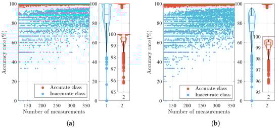
Figure 10.
Accuracy test results of 3629 newly generated samples. (a) RA; (b) DEC.
Furthermore, the classification results of 905018 measurements (3629 samples, with each sample containing 121–361 measurements) are shown in Table 8 and Table 9. The true positive rate (TPR) and false negative rate (FNR) represent the percentages of all the measurements belonging to each class that are correctly and incorrectly classified, respectively. The TPRs of the accurate and inaccurate classes are approximately 99.6% and 87%, respectively. The overall accuracies are higher than 99%. These results mean that it is almost impossible for the trained networks to wrongly identify an accurate measurement as inaccurate, whereas they may miss approximately 13% of the inaccurate measurements.
Table 8.
Accuracy test results of RA BiLSTM (overall accuracy = 99.0633%).
Table 9.
Accuracy test results of DEC BiLSTM (overall accuracy = 99.0039%).
Finally, two regular unidirectional LSTMs, i.e., a forward LSTM and a backward LSTM, are trained using the same training dataset, with the time histories of the validation losses and the TPRs shown in Figure 11 and Table 10, respectively. The number of hidden layers, the number of neurons, and the activation function of the forward and backward LSTMs are the same as those in the modified BiLSTM network. The validation losses and the TPRs of the modified BiLSTM network are plotted in Figure 11 and Table 10 as a comparison. Several interesting properties of the modified BiLSTM network in general can be seen from Figure 11 and Table 10. First, the BiLSTM network has a smaller validation loss and higher TPRs than the other two unidirectional LSTMs, indicating that the bidirectional structure has a better classification capacity. The second is that BiLSTM converges slower than the forward and backward LSTMs, as the bidirectional structure is more complex than the forward and backward structures. Although the BiLSTM has better training convergence and better accuracy, it requires more computational burden when training. In this work, the computational time of training a BiLSTM is approximately 2 times the computational time of training a unidirectional LSTM.
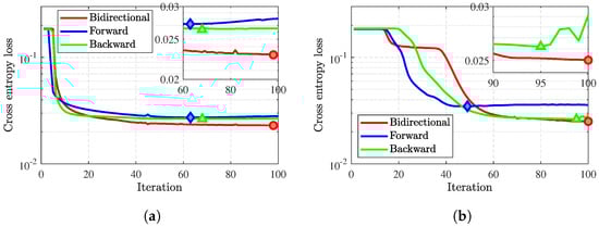
Figure 11.
Validation losses of the bidirectional LSTM, forward LSTM, and backward LSTM. The minimal validation MCEs of the three LSTMs are represented by the red circle, blue diamond, and green triangle, respectively. (a) RA; (b) DEC.
Table 10.
True positive rate results of different network structures.
3.5. Overall Methodology
Using the trained modified BiLSTM networks, inaccurate measurements can be detected. Then, a method is proposed to compensate for these inaccurate measurements to improve OD accuracy. Take the epoch as an instance. If the RA is classified as inaccurate (i.e., the measurement error exceeds ), the following operation is implemented:
where represents the relative measurement error of RA and denotes the sign function, expressed as
In addition, if DEC is detected as inaccurate, the DEC is compensated using
where represents the relative measurement error of DEC.
The reason for using Equations (23)–(25) is that, although the relative measurement errors are not equivalent to the true ones, they should have the same signs. Therefore, the signs of the relative measurement errors are employed to provide the directions of the measurement compensation. Moreover, the magnitudes of the measurement compensation are set as the STD of the measurement error. This is because, although the overall accuracies of the trained modified BiLSTM networks are higher than 99%, a few measurements belonging to the accurate class are still incorrectly classified. These incorrectly classified measurements have true measurements smaller than (i.e., two times the STD of measurement errors). Thus, the magnitude of one STD is used to avoid negative influences from those incorrectly classified measurements.
In this paper, the LSM using BiLSTM-based inaccurate measurement detection is denoted as BiLSTM-LSM. The overall procedure of the proposed BiLSTM-LSM for improving OD accuracy is shown in Algorithm 2. The optimal estimations obtained by the LSM with and without BiLSTM-based inaccurate measurement detection are distinguished using the superscripts ‘BiLSTM-LSM’ and ‘LSM’.
| Algorithm 2: Pseudocode of the proposed method |
|
4. Numerical Simulation
In this section, a cislunar periodic orbit case is investigated to show the advantages of the proposed BiLSTM-LSM in improving OD accuracy. The nominal orbit is a 4:1 synodic resonant NRHO. Note that the 4:1 NRHO is not used in the training or validation datasets. Thus, it is easier to show the generalization capacity of the proposed method in scenarios that have not been trained. In this work, the MATLAB (version R2022a) is employed to generate samples, carry out the estimation process, and plot results, and PyCharm (Python 3.10) is employed to construct and train the neural networks.
4.1. Scenario Descriptions
The nominal 4:1 synodic resonant NRHOs are shown in Figure 12, where the solid red line and blue dots represent the nominal obit and the visible arcs, respectively. The beginning epoch of the OD simulation is selected from a perilune of the 4:1 synodic resonant NRHO. The initial epoch and the associated initial state in the ECI coordinate are listed in Table 11. The measurement duration and the number of measurements are set as 6 h and 361, respectively.
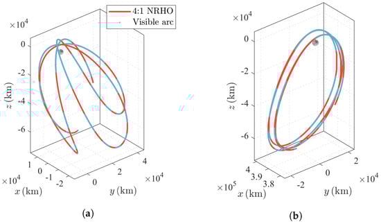
Figure 12.
The 4:1 synodic resonant NRHO. (a) Moon-centered inertial frame; (b) Earth–Moon rotating frame.
Table 11.
Parameters of the simulated case.
4.2. Simulation Results
Three hundred Monte Carlo (MC) runs are performed using both LSM and the proposed BiLSTM-LSM methods. For each MC run, the intervals between two successive measurements and the true measurement errors are randomly generated. In addition, the initial estimated errors are generated using the bounds listed in Table 5. The MC simulation results of the conventional LSM and the proposed BiLSTM-LSM methods are summarized in Figure 13. In Figure 13, and denote the position and velocity estimated errors, respectively. The projections of -, - and - of 300 MC runs are represented using the scatters in Figure 13a, Figure 13b and Figure 13c, respectively. In addition, the ellipses of the 300 estimated errors of the LSM and BiLSTM-LSM methods and the violin plots of each variable are provided in Figure 13. As seen in Figure 13, the ellipses of the proposed BiLSTM-LSM are smaller than those of the LSM method, showing that the estimated errors are reduced using the proposed methods.
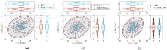
Figure 13.
Monte Carlo simulation results (when the measurement duration is 6 h). (a) Projection of -; (b) projection of -; (c) projection of -.
Furthermore, 300 MC simulations are performed for cases with different measurement durations to illustrate the dependency of the method performance on the measurement durations. Five cases, with measurement durations of 2, 3, 4, and 5 h, are simulated. The number of measurements of these five cases are set to 121, 181, 241, and 301, respectively. Two individual metrics, the position-estimated STD and the velocity-estimated STD , are defined as
where , , , , and are the STDs of , , , , and of the 300 MC runs, respectively.
The 300 MC results of the case when the measurement duration is 2 h are shown in Figure 14, and the results for all six cases are compared in Table 12 and Figure 15. The estimation errors decrease as the measurement durations increase. For example, the position-estimated STDs of the two methods are larger than 100 km when the measurement duration is 2 h, whereas the position-estimated STDs are reduced to approximately 14 km when the measurement duration increases to 6 h. Additionally, Figure 15 shows that the OD accuracy is improved using the proposed BiLSTM-LSM method in all six cases.
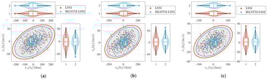
Figure 14.
Monte Carlo simulation results (when the measurement duration is 2 h). (a) Projection of -; (b) projection of -; (c) projection of -.
Table 12.
Estimated STDs comparison results.
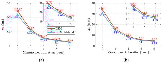
Figure 15.
Monte Carlo simulation results with different measurement durations. (a) Position-estimated STD; (b) velocity-estimated STD.
Moreover, the reduced ratios of the proposed BiLSTM-LSM methods are provided in Figure 16. The reduced ratio is defined as
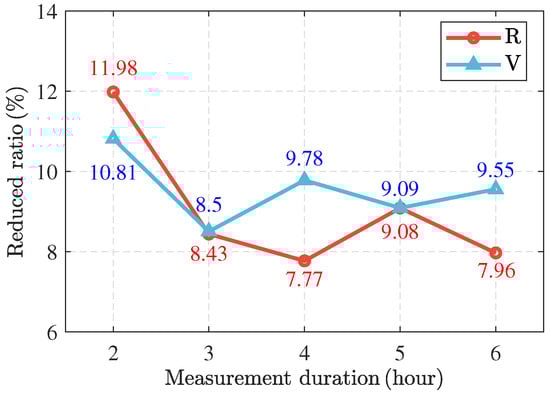
Figure 16.
Reduced ratios of using the proposed BiLSTM-LSM.
As shown in Figure 16, the proposed BiLSTM-LSM method can reduce the estimated errors by approximately 10%. When the measurement duration is 2 h, the reduced ratios in position and velocity are 11.99% and 10.82%, respectively, whereas when the measurement duration is 6 h, the reduced ratios in position and velocity are 7.97% and 9.56%, respectively. Compared with the case of 2 h, the OD improvement performance of the proposed BiLSTM-LSM in the case of 6 h is worse, which is expected since the negative influences of the anomalous measurements are weaker when more measurements are available. However, as shown in Figure 16, the relationship between the measurement duration and the improvement performance is weak. This is because the outputs of the neural network are usually unexplainable, and more results are expected to be analyzed in future work.
Finally, the proposed BiLSTM-LSM is compared with the least sum of absolute residuals (LSAR) method [], which is capable of rejecting outlier measurements when estimating the states. Different from the LSM (Equations (9) and (10)), the LSAR method obtains the optimal solution by solving a linear programming problem (LPP), given by
where
In this work, the LPP in Equations (29)–(33) are solved using the solver MOSEK (https://www.mosek.com, accessed on 3 September 2024) with its interior point algorithm. The initial state is iteratively estimated and the convergence conditions are set as the same as the LSM in Algorithm 1. Three hundred MC runs are carried out for the LSAR method, and the corresponding estimated position and velocity STDs are listed in Table 12. It can be seen from Table 12 that the proposed method obtains more accurate estimations than the LSAR method. The estimations of the LSAR method are even worse than those of the LSM. This is because the LSAR is particularly designed for addressing outlier measurements that have large errors (larger than ten times the measurement STDs). The LSAR performs worse than the standard LSM when none of the measurements are outliers [] (note that the inaccurate measurements defined in this paper are not outliers), which is, of course, worse than the proposed method.
5. Conclusions
In this paper, a bidirectional long short-term memory (BiLSTM) network-based approach is proposed to improve orbit termination (OD) accuracy. Inaccurate measurements are classified using the designed modified BiLSTM network. After compensating for these inaccurate measurements, a more accurate OD solution is then obtained. The training results show that the overall classification accuracy of the designed modified BiLSTM network is higher than 99%. Compared with the regular unidirectional LSTM networks, the designed modified BiLSTM network has a smaller validation loss and higher predicted accuracy. The proposed method is applied to solve the OD problem of a 4:1 synodic resonant near-rectilinear halo orbit, which is not included in the training and validation dataset. Numerical simulations show that the proposed method can provide a more accurate OD solution than the conventional least square method (LSM), with the estimated errors reduced by 7–12%. Although the LSM is used in this paper, the proposed modified BiLSTM network can be generalized to other systems with different orbit estimation methods by directly replacing the LSM with the corresponding orbit estimation method. In the future, the performances of the proposed method can be validated under different dynamics and measurement models to investigate if such a method can improve OD accuracy in other scenarios. In addition, only Gaussian-distributed measurement errors are considered; thus, it is necessary to further investigate whether the proposed method can improve OD accuracy when non-Gaussian measurement errors (e.g., measurement system errors) exist.
Author Contributions
Methodology, Z.Z. (Zhe Zhang); Writing—review & editing, Y.S.; Supervision, Z.Z. (Zuoxiu Zheng). All authors have read and agreed to the published version of the manuscript.
Funding
This work was supported by the National Natural Science Foundation of China (No. 62394353, No. 12150008) and the Beijing Institute of Technology Research Fund Program for lnnovative talents (No. 2022CX01008).
Data Availability Statement
The original contributions presented in the study are included in the article, further inquiries can be directed to the corresponding author.
Acknowledgments
Thanks to Dong Qiao for providing theoretical guidance.
Conflicts of Interest
The authors declare no conflict of interest.
References
- Abusali, P.A.; Tapley, B.D.; Schutz, B.E. Autonomous navigation of global positioning system satellites using cross-link measurements. J. Guid. Control Dyn. 1998, 21, 321–327. [Google Scholar] [CrossRef]
- Zhou, X.; Qiao, D.; Macdonald, M. Orbit Determination for Impulsively Maneuvering Spacecraft Using Modified State Transition Tensor. J. Guid. Control Dyn. 2024, 47, 822–839. [Google Scholar] [CrossRef]
- Li, X.; Scheeres, D.J.; Qiao, D. Bouncing Return Trajectory Design for Precise Lander Deployment to Asteroids. J. Guid. Control Dyn. 2021, 45, 121–137. [Google Scholar] [CrossRef]
- Zhou, X.; Li, X.; Huo, Z.; Meng, L.; Huang, J. Near-Earth Asteroid Surveillance Constellation in the Sun-Venus Three-Body System. Space Sci. Technol. 2022, 2022, 9864937. [Google Scholar] [CrossRef]
- Duong, N.; Winn, C.B. Orbit determination by range-only data. J. Spacecr. Rocket. 1973, 10, 132–136. [Google Scholar] [CrossRef]
- Hill, K.; Born, G.H. Autonomous interplanetary orbit determination using satellite-to-satellite tracking. J. Guid. Control Dyn. 2007, 30, 679–686. [Google Scholar] [CrossRef]
- Hill, K.; Born, G.H. Autonomous orbit determination from lunar halo orbits using crosslink range. J. Spacecr. Rocket. 2008, 45, 548–553. [Google Scholar] [CrossRef]
- Cinelli, M.; Ortore, E.; Mengali, G.; Quarta, A.A.; Circi, C. Lunar orbits for telecommunication and navigation services. Astrodynamics 2024, 8, 209–220. [Google Scholar] [CrossRef]
- Geller, D.K.; Klein, I. Angles-only navigation state observability during orbital proximity operations. J. Guid. Control Dyn. 2014, 37, 1976–1983. [Google Scholar] [CrossRef]
- Qiao, D.; Zhou, X.; Li, X. Analytical configuration uncertainty propagation of geocentric interferometric detection constellation. Astrodynamics 2023, 7, 271–284. [Google Scholar] [CrossRef]
- Li, X.; Qiao, D.; Circi, C. Mars High Orbit Capture Using Manifolds in the Sun–Mars System. J. Guid. Control Dyn. 2020, 43, 1383–1392. [Google Scholar] [CrossRef]
- Qiao, D.; Zhou, X.; Li, X. Configuration uncertainty propagation of gravitational-wave observatory using a directional state transition tensor. Chin. J. Aeronaut. 2024. [Google Scholar] [CrossRef]
- Kedarisetty, S.; Shima, T. Sinusoidal Guidance. J. Guid. Control Dyn. 2023, 47, 1–16. [Google Scholar] [CrossRef]
- Han, H.; Li, X.; Qiao, D. Aerogravity-assist capture into the three-body system: A preliminary design. Acta Astronaut. 2022, 198, 26–35. [Google Scholar] [CrossRef]
- Chen, J.; Qiao, D.; Han, H. Augmented Analytical Aerocapture Guidance by Segmented State Approximation. J. Guid. Control Dyn. 2024, 1–12. [Google Scholar] [CrossRef]
- Li, X.; Warier, R.R.; Sanyal, A.K.; Qiao, D. Trajectory Tracking Near Small Bodies Using Only Attitude Control. J. Guid. Control Dyn. 2018, 42, 109–122. [Google Scholar] [CrossRef]
- Li, X.; Qiao, D.; Macdonald, M. Energy-saving capture at mars via backward-stable orbits. J. Guid. Control Dyn. 2019, 42, 1136–1145. [Google Scholar] [CrossRef]
- Yao, Q.; Han, H.; Qiao, D. Nonsingular Fixed-Time Tracking Guidance for Mars Aerocapture with Neural Compensation. IEEE Trans. Aerosp. Electron. Syst. 2022, 58, 3686–3696. [Google Scholar] [CrossRef]
- Luo, Y.; Qin, T.; Zhou, X. Observability Analysis and Improvement Approach for Cooperative Optical Orbit Determination. Aerospace 2022, 9, 166. [Google Scholar] [CrossRef]
- Qiao, D.; Zhou, X.; Zhao, Z.; Qin, T. Asteroid Approaching Orbit Optimization Considering Optical Navigation Observability. IEEE Trans. Aerosp. Electron. Syst. 2022, 58, 5165–5179. [Google Scholar] [CrossRef]
- Fossà, A.; Losacco, M.; Armellin, R. Perturbed initial orbit determination. Astrodynamics 2024, 1–16. [Google Scholar] [CrossRef]
- Cao, Z.; Li, X.; Qi, Y. Semi-Analytical Assessment of Multiple Gravity-Assist Opportunities Based on Feasibility Domains. J. Guid. Control Dyn. 2024, 47, 1645–1659. [Google Scholar] [CrossRef]
- Zhou, X.; Qin, T.; Macdonald, M.; Qiao, D. Observability analysis of cooperative orbit determination using inertial inter-spacecraft angle measurements. Acta Astronaut. 2023, 210, 289–302. [Google Scholar] [CrossRef]
- Park, R.S.; Scheeres, D.J. Nonlinear semi-analytic methods for trajectory estimation. J. Guid. Control Dyn. 2007, 30, 1668–1676. [Google Scholar] [CrossRef]
- Zhang, S.; Fu, T.; Chen, D.; Ding, S.; Gao, M. An Initial Orbit Determination Method Using Single-Site Very Short Arc Radar Observations. IEEE Trans. Aerosp. Electron. Syst. 2020, 56, 1856–1872. [Google Scholar] [CrossRef]
- Zhou, X.; Jia, F.; Li, X. Configuration Stability Analysis for Geocentric Space Gravitational-Wave Observatories. Aerospace 2022, 9, 519. [Google Scholar] [CrossRef]
- Kaufman, E.; Lovell, T.A.; Lee, T. Nonlinear observability for relative orbit determination with angles-only measurements. J. Astronaut. Sci. 2016, 63, 60–80. [Google Scholar] [CrossRef]
- Julier, S.J.; Uhlmann, J.K. Unscented filtering and nonlinear estimation. Proc. IEEE 2004, 92, 401–422. [Google Scholar] [CrossRef]
- Chang, L.; Hu, B.; Li, A.; Qin, F. Transformed unscented kalman filter. IEEE Trans. Autom. Control 2013, 58, 252–257. [Google Scholar] [CrossRef]
- Arasaratnam, I.; Haykin, S. Cubature kalman filters. IEEE Trans. Autom. Control 2009, 54, 1254–1269. [Google Scholar] [CrossRef]
- Jia, B.; Xin, M.; Cheng, Y. High-degree cubature Kalman filter. Automatica 2013, 49, 510–518. [Google Scholar] [CrossRef]
- Zhang, L.; Yang, H.; Lu, H.; Zhang, S.; Cai, H.; Qian, S. Cubature Kalman filtering for relative spacecraft attitude and position estimation. Acta Astronaut. 2014, 105, 254–264. [Google Scholar] [CrossRef]
- Adurthi, N.; Singla, P. Conjugate unscented transformation-based approach for accurate conjunction analysis. J. Guid. Control Dyn. 2015, 38, 1642–1658. [Google Scholar] [CrossRef]
- Nanda, A.; Singla, P.; Karami, M.A. Conjugate unscented transformation–based uncertainty analysis of energy harvesters. J. Intell. Mater. Syst. Struct. 2018, 29, 3614–3633. [Google Scholar] [CrossRef] [PubMed]
- Luo, Y.; Yang, Z. A review of uncertainty propagation in orbital mechanics. Prog. Aerosp. Sci. 2017, 89, 23–39. [Google Scholar] [CrossRef]
- Qiao, D.; Zhou, X.; Li, X. Feasible domain analysis of heliocentric gravitational-wave detection configuration using semi-analytical uncertainty propagation. Adv. Space Res. 2023, 72, 4115–4131. [Google Scholar] [CrossRef]
- Shang, H.; Liu, Y. Assessing accessibility of main-belt asteroids based on Gaussian process regression. J. Guid. Control Dyn. 2017, 40, 1144–1154. [Google Scholar] [CrossRef]
- Sun, Z.; Simo, J.; Gong, S. Satellite Attitude Identification and Prediction Based on Neural Network Compensation. Space Sci. Technol. 2023, 3, 9. [Google Scholar] [CrossRef]
- Xu, L.; Zhang, G.; Qiu, S.; Cao, X. Optimal Multi-impulse Linear Rendezvous via Reinforcement Learning. Space Sci. Technol. 2023, 3, 47. [Google Scholar] [CrossRef]
- Li, H.; Chen, S.; Izzo, D.; Baoyin, H. Deep networks as approximators of optimal low-thrust and multi-impulse cost in multitarget missions. Acta Astronaut. 2020, 166, 469–481. [Google Scholar] [CrossRef]
- Gao, T.; Peng, H.; Bai, X. CaLibration of atmospheric density model based on Gaussian Processes. Acta Astronaut. 2020, 168, 273–281. [Google Scholar] [CrossRef]
- Yang, B.; Li, S.; Feng, J.; Vasile, M. Fast Solver for J2-Perturbed Lambert Problem Using Deep Neural Network. J. Guid. Control Dyn. 2022, 45, 875–884. [Google Scholar] [CrossRef]
- Peng, H.; Bai, X. Improving orbit prediction accuracy through supervised machine learning. Adv. Space Res. 2018, 61, 2628–2646. [Google Scholar] [CrossRef]
- Peng, H.; Bai, X. Artificial neural network-based machine learning approach to improve orbit prediction accuracy. J. Spacecr. Rocket. 2018, 55, 1248–1260. [Google Scholar] [CrossRef]
- Peng, H.; Bai, X. Gaussian Processes for improving orbit prediction accuracy. Acta Astronaut. 2019, 161, 44–56. [Google Scholar] [CrossRef]
- Peng, H.; Bai, X. Comparative evaluation of three machine learning algorithms on improving orbit prediction accuracy. Astrodynamics 2019, 3, 325–343. [Google Scholar] [CrossRef]
- Peng, H.; Bai, X. Fusion of a machine learning approach and classical orbit predictions. Acta Astronaut. 2021, 184, 222–240. [Google Scholar] [CrossRef]
- Peng, H.; Bai, X. Machine Learning Approach to Improve Satellite Orbit Prediction Accuracy Using Publicly Available Data. J. Astronaut. Sci. 2020, 67, 762–793. [Google Scholar] [CrossRef]
- Li, B.; Huang, J.; Feng, Y.; Wang, F.; Sang, J. A Machine Learning-Based Approach for Improved Orbit Predictions of LEO Space Debris with Sparse Tracking Data From a Single Station. IEEE Trans. Aerosp. Electron. Syst. 2020, 56, 4253–4268. [Google Scholar] [CrossRef]
- Zhou, X.; Qin, T.; Meng, L. Maneuvering Spacecraft Orbit Determination Using Polynomial Representation. Aerospace 2022, 9, 257. [Google Scholar] [CrossRef]
- Zhou, X.; Qin, T.; Ji, M.; Qiao, D. A LSTM assisted orbit determination algorithm for spacecraft executing continuous maneuver. Acta Astronaut. 2022, 204, 568–582. [Google Scholar] [CrossRef]
- Zhou, X.; Qiao, D.; Li, X. Neural Network-Based Method for Orbit Uncertainty Propagation and Estimation. IEEE Trans. Aerosp. Electron. Syst. 2024, 60, 1176–1193. [Google Scholar] [CrossRef]
- Zhou, X.; Wang, S.; Qin, T. Multi-Spacecraft Tracking and Data Association Based on Uncertainty Propagation. Appl. Sci. 2022, 12, 7660. [Google Scholar] [CrossRef]
- Zhou, X.; Cheng, Y.; Qiao, D.; Huo, Z. An adaptive surrogate model-based fast planning for swarm safe migration along halo orbit. Acta Astronaut. 2022, 194, 309–322. [Google Scholar] [CrossRef]
- Zhou, X.; Li, X.; Zhang, Z. Neural Network–Assisted Initial Orbit Determination Method for Libration Point Orbits. J. Aerosp. Eng. 2024, 37, 4024046. [Google Scholar] [CrossRef]
- Schuster, M.; Paliwal, K. Bidirectional recurrent neural networks. IEEE Trans. Signal Process. 1997, 45, 2673–2681. [Google Scholar] [CrossRef]
- Bonet, I.; Rodriguez, A.; Grau, I. Bidirectional Recurrent Neural Networks for Biological Sequences Prediction BT—Advances in Soft Computing and Its Applications; Springer: Berlin/Heidelberg, Germany, 2013; pp. 139–149. [Google Scholar]
- Gouhara, K.; Watanabe, T.; Uchikawa, Y. Learning process of recurrent neural networks. In Proceedings of the 1991 IEEE International Joint Conference on Neural Networks, Singapore, 18–21 November 1991; Volume 1, pp. 746–751. [Google Scholar] [CrossRef]
- Boden, M.; Hawkins, J. Improved access to sequential motifs: A note on the architectural bias of recurrent networks. IEEE Trans. Neural Netw. 2005, 16, 491–494. [Google Scholar] [CrossRef] [PubMed]
- Hochreiter, S.; Schmidhuber, J. Long Short-Term Memory. Neural Comput. 1997, 9, 1735–1780. [Google Scholar] [CrossRef]
- Greff, K.; Srivastava, R.K.; Koutnik, J.; Steunebrink, B.R.; Schmidhuber, J. LSTM: A Search Space Odyssey. IEEE Trans. Neural Netw. Learn. Syst. 2017, 28, 2222–2232. [Google Scholar] [CrossRef]
- Siami-Namini, S.; Tavakoli, N.; Namin, A.S. The Performance of LSTM and BiLSTM in Forecasting Time Series. In Proceedings of the 2019 IEEE International Conference on Big Data (Big Data), Los Angeles, CA, USA, 9–12 December 2019; pp. 3285–3292. [Google Scholar] [CrossRef]
- Hameed, Z.; Garcia-Zapirain, B. Sentiment Classification Using a Single-Layered BiLSTM Model. IEEE Access 2020, 8, 73992–74001. [Google Scholar] [CrossRef]
- Bretagnon, P. Theory for the motion of all the planets-The VSOP82 solution. Astron. Astrophys. 1982, 114, 278–288. [Google Scholar]
- Moisson, X.; Bretagnon, P. Analytical planetary solution VSOP2000. Celest. Mech. Dyn. Astron. 2001, 80, 205–213. [Google Scholar] [CrossRef]
- Han, H.; Li, X.; Ren, J. Transfer between Libration orbits through the outer branches of manifolds for Phobos exploration. Acta Astronaut. 2021, 189, 321–336. [Google Scholar] [CrossRef]
- Ou, Y.; Zhang, H.; Li, B. Absolute orbit determination using line-of-sight vector measurements between formation flying spacecraft. Astrophys. Space Sci. 2018, 363, 1–13. [Google Scholar] [CrossRef]
- Hu, Y.; Sharf, I.; Chen, L. Three-spacecraft autonomous orbit determination and observability analysis with inertial angles-only measurements. Acta Astronaut. 2020, 170, 106–121. [Google Scholar] [CrossRef]
- Hu, Y.; Sharf, I.; Chen, L. Distributed orbit determination and observability analysis for satellite constellations with angles-only measurements. Automatica 2021, 129, 109626. [Google Scholar] [CrossRef]
- Karim, F.; Majumdar, S.; Darabi, H.; Chen, S. LSTM Fully Convolutional Networks for Time Series Classification. IEEE Access 2018, 6, 1662–1669. [Google Scholar] [CrossRef]
- Daniel, J.G. Generating Periodic Orbits in the Circular Restricted Three-Body Problem with Applications to Lunar South Pole Coverage. Ph.D. Thesis, Purdue University, West Lafayette, IN, USA, 2006. [Google Scholar]
- Zhou, X.; Qiao, D.; Li, X. Adaptive Order-Switching Kalman Filter for Orbit Determination Using Deep-Neural-Network-Based Nonlinearity Detection. J. Spacecr. Rocket. 2023, 60, 1724–1741. [Google Scholar] [CrossRef]
- Howell, K.C.; Pernicka, H.J. Numerical determination of Lissajous trajectories in the restricted three-body problem. Celest. Mech. 1987, 41, 107–124. [Google Scholar] [CrossRef]
- Dormand, J.R.; Prince, P.J. A family of embedded Runge-Kutta formulae. J. Comput. Appl. Math. 1980, 6, 19–26. [Google Scholar] [CrossRef]
- Olsson, A.; Sandberg, G.; Dahlblom, O. On Latin hypercube sampling for structural reliability analysis. Struct. Saf. 2003, 25, 47–68. [Google Scholar] [CrossRef]
- Ghiasi-Shirazi, K. Competitive Cross-Entropy Loss: A Study on Training Single-Layer Neural Networks for Solving Nonlinearly Separable Classification Problems. Neural Process. Lett. 2019, 50, 1115–1122. [Google Scholar] [CrossRef]
- Prabhu, K.; Majji, M.; Alfriend, K.T. Least Sum of Absolute Residuals Orbit Determination. J. Guid. Control Dyn. 2022, 45, 468–480. [Google Scholar] [CrossRef]
Disclaimer/Publisher’s Note: The statements, opinions and data contained in all publications are solely those of the individual author(s) and contributor(s) and not of MDPI and/or the editor(s). MDPI and/or the editor(s) disclaim responsibility for any injury to people or property resulting from any ideas, methods, instructions or products referred to in the content. |
© 2024 by the authors. Licensee MDPI, Basel, Switzerland. This article is an open access article distributed under the terms and conditions of the Creative Commons Attribution (CC BY) license (https://creativecommons.org/licenses/by/4.0/).