A Small-Scale Landslide in 2023, Leshan, China: Basic Characteristics, Kinematic Process and Cause Analysis

Abstract

Sudden mountain landslides can pose substantial threats to human lives and property. On 4 June 2023, a landslide occurred in Jinkouhe District, Leshan City, Sichuan Province, resulting in 19 deaths and 5 injuries. This study, drawing on field investigations, geological data, and historical imagery, elucidates the characteristics and causes of the landslide and conducts a reverse analysis of the landslide movement process using Massflow V2.8 numerical simulation software. The results indicate that rainfall and human engineering activities are key factors that triggered this landslide. Numerical simulation shows that the landslide stopped after 60 s of sliding, with a movement distance of approximately 286 m, a maximum sliding speed of 17 m/s, and a maximum accumulation thickness of 7 m, eventually forming a loose landslide debris accumulation of approximately 5.25 × 10³ m³. The findings of this study provide significant reference value for research on landslide movement characteristics and disaster prevention and mitigation in mountainous areas.

1. Introduction

Landslides are common geological hazards that cause significant damage to individuals, society, and the environment [1]. They also significantly accelerate ecosystem degradation and desertification. The occurrence of landslides depends on local conditions (such as topography and lithology), meteorological and hydrological conditions, and may also be influenced by rainfall [2,3,4], earthquakes [5,6], typhoons [7], floods [8,9], snowmelt [10], and human engineering activities [11,12,13]. Sometimes, multiple factors may jointly contribute to landslides [14,15].

Catastrophic landslides often exhibit hidden and sudden characteristics. With the increase in population density and engineering development in mountainous areas, the frequency of disastrous landslides has risen, particularly high-frequency small landslides, which are especially hazardous [16]. Numerous large-scale landslide events are recorded in the Emergency Events Database (EM-DAT) and the “China Statistical Yearbook” [17]. However, due to the lack of on-site monitoring data, real-time disaster parameter acquisition, and predictive data, smaller-scale landslides (<10⁵ m³) are often not recorded. This results in data gaps in landslide risk assessments, complicating disaster prevention and mitigation efforts. Research on the movement processes of landslides is of great significance for understanding landslide mechanisms and formulating effective disaster prevention and mitigation strategies. Both domestic and international scholars have extensively studied landslide movement processes using the discrete element and continuum mechanics methods. Poisel et al. employed PFC3D 3.10 software to study the movement process of a landslide in Peru and verified the accuracy of the simulation results [18]. Roslan et al. indicated that UDEC V6.0 software could simulate the process of rock fracturing and subsequent displacement, making it an essential tool for studying slope stability [19]. While these methods have made significant progress in simulating landslide movement processes, their application scope and accuracy still need further improvement.

In recent years, advances in technology, particularly in remote sensing and Geographic Information Systems (GIS), have introduced new tools and methods for landslide research. Unmanned Aerial Vehicle (UAV) technology, as an emerging remote sensing tool, has been extensively applied in acquiring geospatial data and environmental monitoring due to its efficiency, cost-effectiveness, and flexibility. UAVs can rapidly acquire high-resolution terrain data, thereby providing essential data support for landslide research. For example, Filice et al. integrated field investigations with UAV data to evaluate the stability of rocky slopes, thereby demonstrating further the crucial role of UAV technology in terrain analysis [20]. Schilirò et al. employed UAV technology to examine landslides induced by earthquakes in central Italy, underscoring the significant role of UAVs in real-time monitoring and data acquisition [21]. Additionally, digital terrain models (DTM) generated by UAVs are invaluable for real-time monitoring and geological disaster assessment and for the accurate simulation of landslide accumulation areas. Niethammer et al. used high-precision DTM data to investigate the Super-Sauze landslide event, demonstrating the utility of UAV technology for detailed dynamic monitoring of landslides and elucidating the impact of terrain changes on landslide accumulation areas [22]. Massaro et al. conducted a study in a volcanic structural area, utilizing DTM data generated by UAVs to simulate rockfall trajectories, thereby showcasing their potential applications in geological hazard monitoring [23]. These studies indicate that high-resolution DTM data are indispensable for landslide research, offering substantial support for a comprehensive understanding of landslide mechanisms and disaster prevention.

In this context, Ouyang et al. developed the Massflow numerical software based on the theory of deep continuous integration, which has been successfully applied to multiple landslide cases. For instance, Ouyang et al. demonstrated the effectiveness of Massflow in dynamic analysis and landslide prediction through numerical simulations of the Shenzhen Guangming New District landslide [24]. Scaringi et al. conducted detailed numerical simulations using Massflow software to study the Xinmo Village landslide in Mao County, revealing the triggering mechanisms and movement processes of the landslide and proposed new methods for landslide risk assessment [25]. Fan et al. performed comprehensive numerical simulations of multi-hazard chains using Massflow software to study the Baige landslide in the Jinsha River, predicting possible development trends and disaster impacts [26]. Massflow has achieved notable application results in simulating the movement process of landslides, hazard assessment, and risk evaluation [27]. It has been widely used in the research of the dynamic evolution processes of mountain disasters. As UAV technology continues to advance, the precision and efficiency of generated DTM are continuously improving. This advancement provides more reliable and detailed terrain information support for Massflow and other simulation software, further promoting the development and application of landslide movement process simulations.

Around 4 a.m. on 4 June 2023 (UTC+8), a small, catastrophic landslide occurred in Yongsheng Township, Jinkouhe District, Leshan City, Sichuan Province, China (hereinafter referred to as the Yongsheng landslide). Landslides frequently occur in mountainous geological environments, posing serious threats to the safety of local residents and their property. Therefore, studying the developmental characteristics and triggering factors of landslides is of considerable scientific and practical importance. Using the Yongsheng landslide as a case study, this research involved a detailed field investigation to record the primary developmental characteristics of the landslide, including its scale, morphology, and sliding direction. Additionally, a systematic analysis of the landslide’s triggering mechanisms was performed by considering various factors such as topography, rainfall, and human engineering activities. High-resolution images and surface deformation data of the landslide at various periods were acquired through historical landslide images, UAV aerial photography, and InSAR deformation analysis, providing abundant foundational data for studying the instability characteristics of the landslide. On this basis, a Massflow numerical model was developed to perform a quantitative analysis of the landslide’s movement speed and final accumulation configuration. Numerical simulations elucidated the principles of energy conversion and material transport during the landslide process. These findings not only enhance the understanding of the causes and dynamic processes of landslides but also provide a scientific foundation for the development of future landslide disaster monitoring and early warning systems.

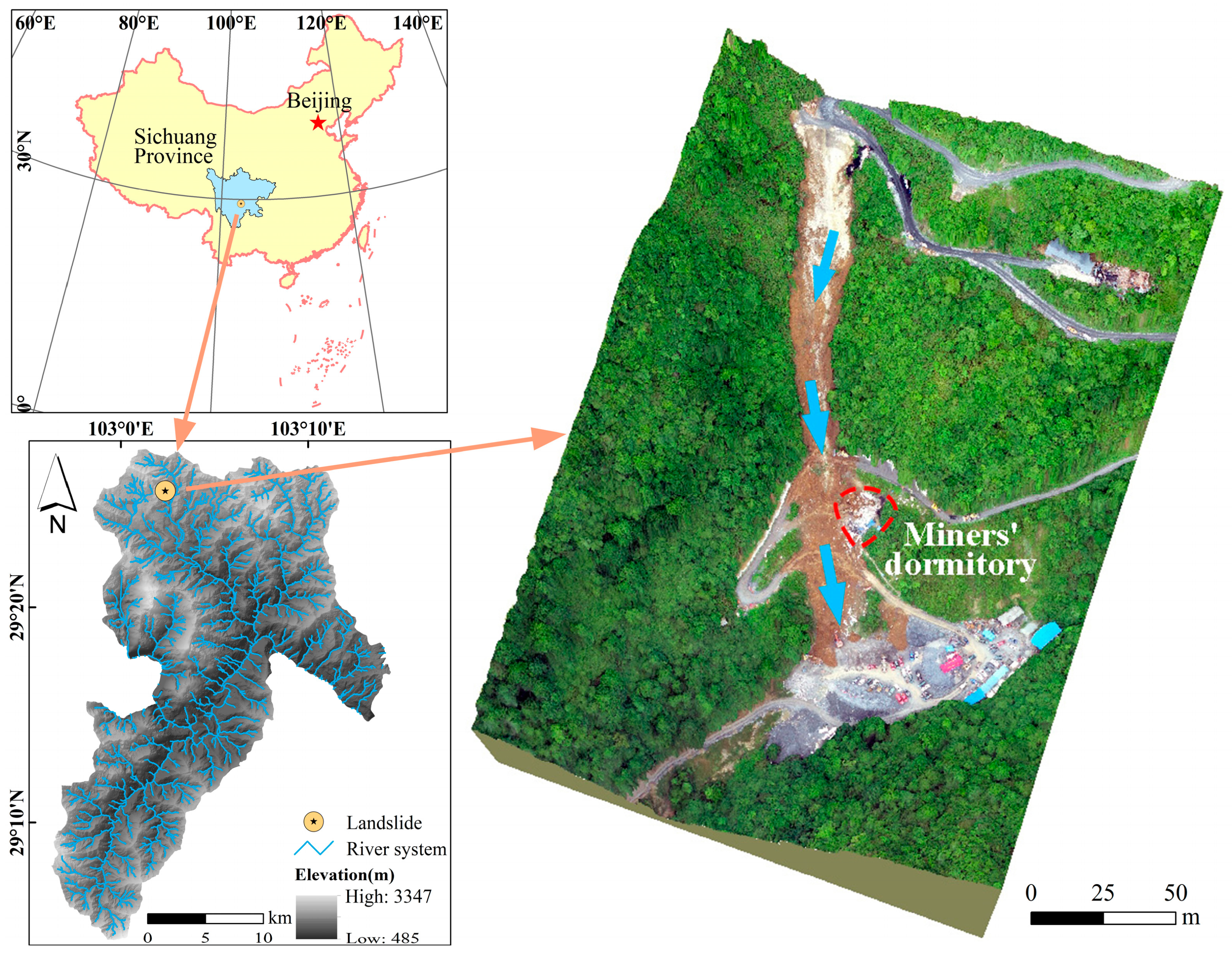
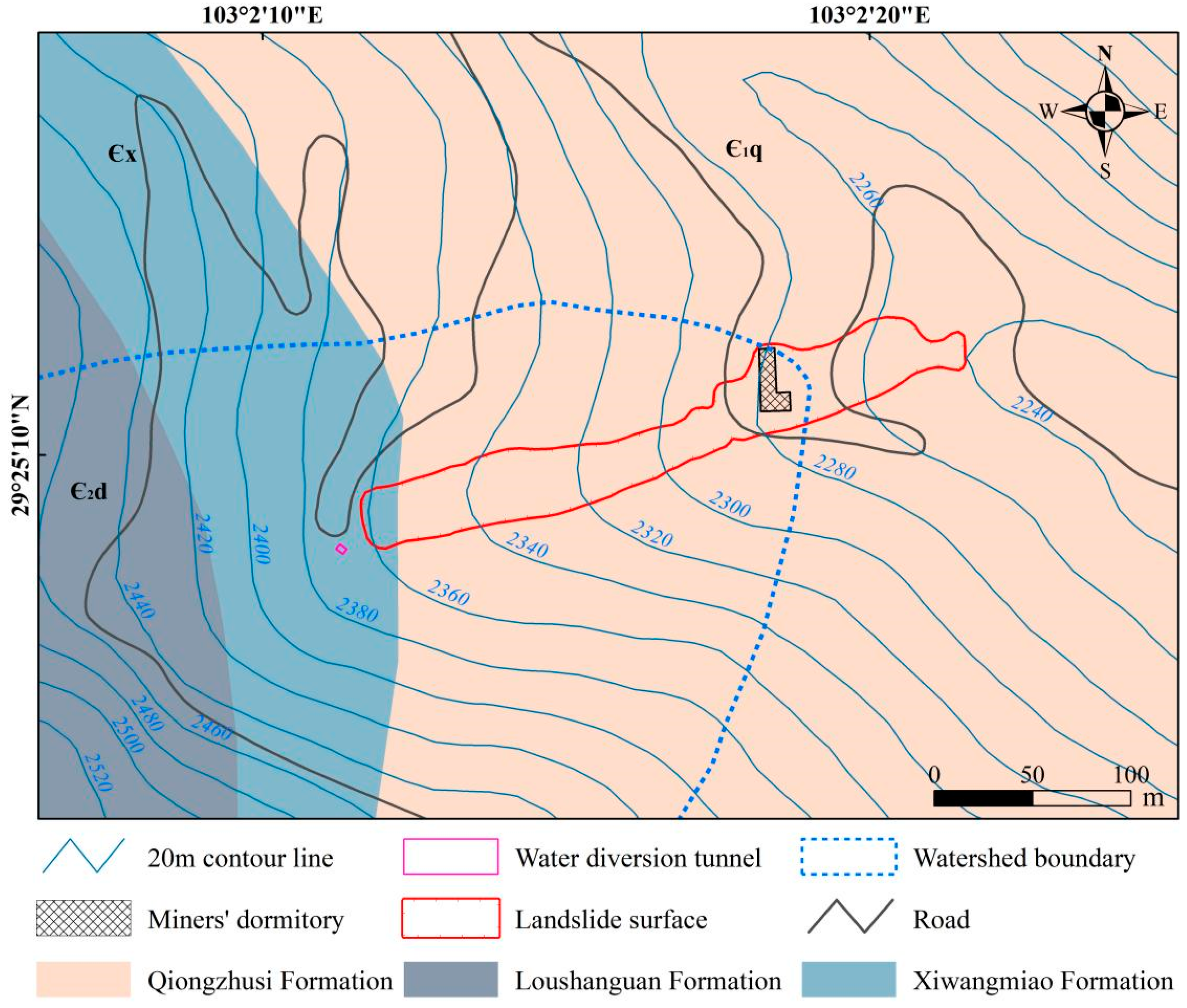
2. Overview of the Landslide Area

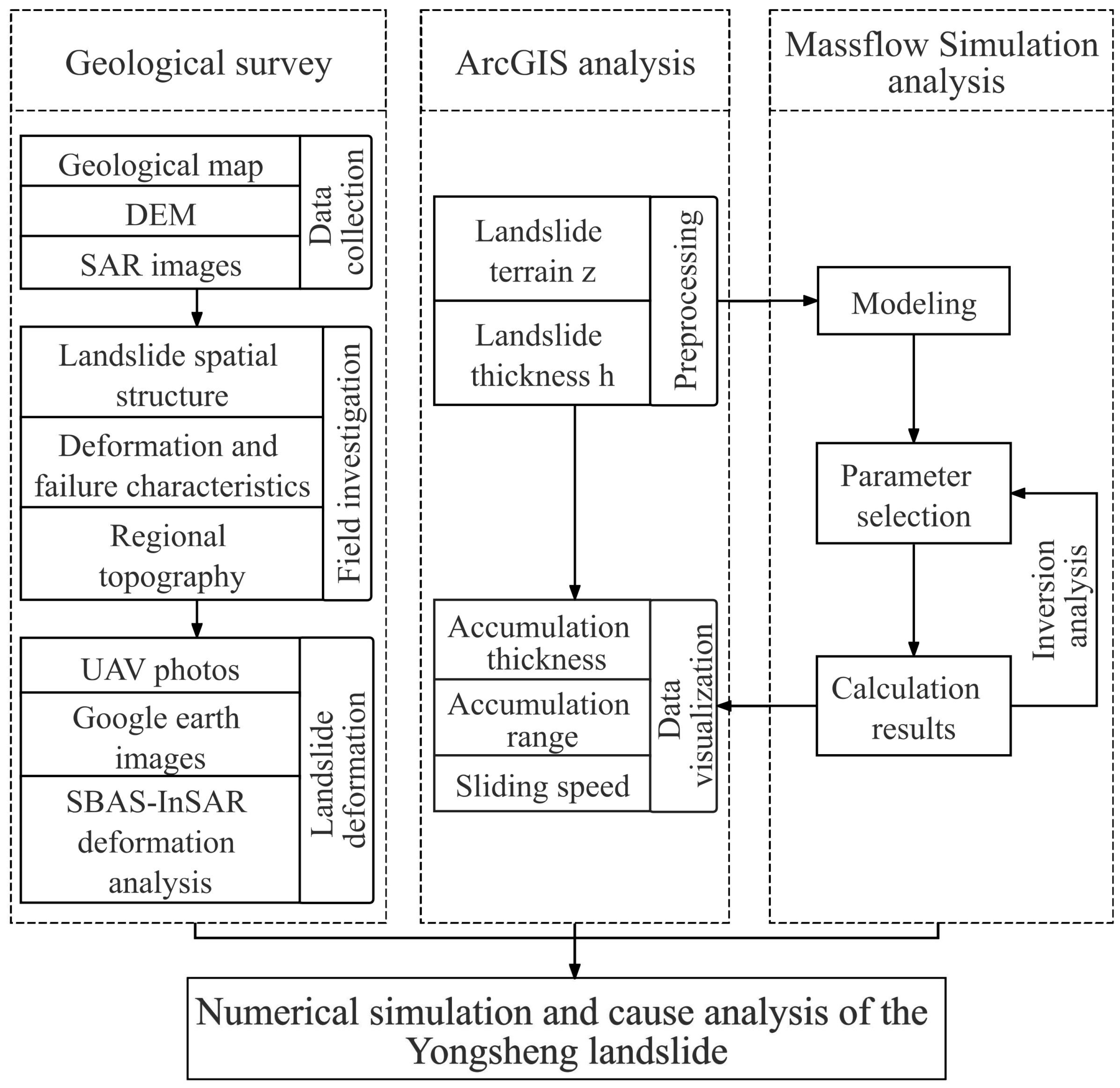
The Yongsheng landslide is located in Yongsheng Township, Sichuan Province, at geographical coordinates of 103°2′25.75′′E and 29°25′0.6′′N. This area has abundant water systems and an elevation above 2000 m a.s.l., with the overall terrain trending higher in the southwest and lower in the northeast. The maximum elevation is 3347 m, and the minimum elevation is 485 m (Figure 1).

The landslide area is situated in the transitional zone between the eastern edge of the Qinghai–Tibet Plateau and the Sichuan Basin, characterized by complex geological structures including folds, faults, and fracture zones. Crustal uplift and river erosion have resulted in the formation of steep terrain, significantly impacting landslide activity. The stratigraphy of the gully catchment area where the Yongsheng landslide is located can be divided into two sections: the upper section is part of the Middle Cambrian Louzhanguan Formation (Є₂d), while the lower section consists of the Lower Cambrian Xiwangmiao Formation (Єx) and Qiongzhusi Formation (Є₁q) (Figure 2). Among these, the water diversion tunnel located on the right side of the landslide’s rear edge is within the Xiwangmiao Formation. This tunnel extends to a depth of approximately 57 m, and the lithology at the tunnel entrance is dolomite. The strata of the Xiwangmiao and Qiongzhusi Formations have a dip direction of 110°–120° and a dip angle of 10°–30°. The rock mass features well-developed fractures that divide it into blocks, resulting in fragmentation. According to field investigations, the main material of the landslide body is Quaternary Holocene residual slope deposits (Q₄^el+dl), primarily composed of gravelly silty clay.

The region where the Yongsheng landslide occurred is characterized by a subtropical monsoon climate featuring mild temperatures, abundant rainfall, and significant freeze-thaw action. Figure 3 depicts the daily and cumulative rainfall in Leshan City. The figure shows that the area experienced continuous heavy rainfall in the month preceding the landslide, with the highest daily rainfall reaching 31.23 mm and the cumulative rainfall totaling 159.75 mm.

3. Data and Methods

3.1. Data

The data used in this study includes the 1:200,000 geological maps provided by the China Geological Survey (http://www.ngac.org.cn/, accessed on 4 February 2024); The 12.5 m resolution digital elevation model (DEM) provided by the Advanced Land Observing Satellite (ALOS) of Japan (https://search.asf.alaska.edu, accessed on 22 February 2024); Landslide photos are sourced from UAV images, on-site photography, and 0.6 m resolution Google Earth imagery. Rainfall data were obtained from the 2023 meteorological data provided by the National Centers for Environmental Information under the National Oceanic and Atmospheric Administration (NOAA) (https://www.ncei.noaa.gov/data/global-summary-of-the-day/archive/, accessed on 23 February 2024). The SAR imagery data are the ascending orbit Sentinel-1A satellite images of the area before the landslide occurred (https://search.asf.alaska.edu, accessed on 2 March 2024).

3.2. Methods

3.2.1. Methods for Analyzing Pre-Landslide Deformation

This study conducted detailed field investigations of various areas of the landslide and its surrounding environment, gaining an understanding of the region’s environment, geomorphology, geological structures, rock and soil characteristics, and the scale, extent, and morphological features of the collapse zone. To analyze the dynamic changes of the landslide, this study utilized multiple high-resolution satellite images from Google Earth, obtained prior to the landslide, to systematically assess the geomorphological changes in the vicinity.

Additionally, employing Short Baseline Subset Interferometric Synthetic Aperture Radar (SBAS-InSAR) technology [28], 22 ascending track Sentinel-1A radar images acquired before the landslide event, spanning from 2 September 2022 to 24 May 2023, were obtained. The parameters of the data are presented in

Table 1. Sentinenl-1A data parameters.

Orbital Direction	Imaging Mode	Band	Wavelength/m	Resolution/m	Polarization Mode	Number/Scene	Processing Method
Ascending orbit	IW	C	5.63	5 × 20	VV	22	SBAS-InSAR

. Through a time-series analysis, surface displacement changes in the landslide area were monitored, revealing deformation characteristics and rates preceding the landslide event.

To improve the accuracy of SBAS-InSAR interferometry and reduce errors caused by phase discontinuities in the interferogram, this study selected 22 precision orbit datasets of Sentinel-1A encompassing periods before and after the acquisition time of each scene for image correction, generated corresponding single look complex (SLC) images. Subsequently, it cropped the images to the range suitable for the research object. Given the significant topographical variations in the study area, this study utilized global DEM data with a resolution of 12.5 m to mitigate the influence of the topographic phase on the deformation phase. The specific process of SBAS-InSAR is as follows:

• Interferogram Baseline Combination: The Sentinel-1A data, which had been clipped, was processed using SARscape 5.2 software in ENVI to perform interferometric filtering. A total of 101 image pairs were generated, with the temporal and spatial baseline thresholds set at 75 d and 5%, respectively.
• Interferometric Workflow: The entire process includes coherence generation, interferogram flattening, filtering (using the Goldstein filtering method to enhance filtering), and phase unwrapping (using the minimum cost flow method). By setting the multi-look number to 1:4, speckle noise can be effectively suppressed. Setting the unwrapping grade to 2 and the unwrapping threshold to 0.29 ensures sufficient unwrapped data in mountainous areas, thereby removing some noise and reducing data storage requirements.
• Orbit Refinement and Reflattening: Given the complex terrain and numerous mountains in the study area, Google Earth was used to select stable points, such as stable transportation hubs and other structures, as ground control points (GCP) to reduce errors caused by improper point selection.
• SBAS Inversion: This includes estimating deformation rates and residual topography based on the thresholds of the first inversion and optimizing the unwrapped map generated in the second step for subsequent processing.
• Geocoding: By unifying the geographical coordinates of the results from the two inversions, an annual average deformation rate map of the deformation points in the study area was obtained.

3.2.2. Methods for Kinematic Analysis of Landslides

Massflow adopts the principles of depth-integrated continuum mechanics and an improved MacCormack-TVD finite difference method. It is independently programmed using Fortran and C# languages. Based on the conservation of mass and momentum equations, the physical quantities of the Navier–Stokes equations are integrated in the Z direction [23]. The calculation equations can be expressed as (Equations (1) and (2)):

$${\displaystyle \frac{\partial h_1}{\partial t}}+{\displaystyle \frac{\partial h_1{u}_1}{\partial x}}+{\displaystyle \frac{\partial h_1{v}_1}{\partial y}}=0$$

(1)

$${\displaystyle \frac{\partial ({\rho }_1{h}_1{u}_1)}{\partial t}}+{\displaystyle \frac{\partial ({\rho }_1{h}_1{u}_1^2)}{\partial x}}+{\displaystyle \frac{\partial ({\rho }_1{h}_1{u}_h{v}_1)}{\partial v}}={\rho }_1{u}_1{z}_{1bot}{E}_{1bot}-{\tau }_{1zybot}-{\rho }_{1}g{h}_1{\displaystyle \frac{\partial (h_1+z_{1bot})}{\partial x}}$$

(2)

In the equations, ${\rho }_1$ and $h_1$ represent the density and thickness of the top flowing layer; $u_1$ and $v_1$ are the boundary velocities in the $x$ and $y$ directions; ${\tau }_{1zybot}$ is the shear stress of the upper flowing layer on the bottom; $z_{1bot}$ is the basal boundary of the top flowing layer; $E_{1bot}$ is the entrainment rate of the bottom stable layer; $g$ is the gravitational acceleration.

This study utilized UAV photogrammetry to obtain the DEM of the study area. The elevation data from the DEM were converted into an ASCII format file using the conversion tools in ArcGIS and then imported into the Massflow software. In this simulation, the computational model used a 2 × 2 m grid, dividing the landslide calculation area into 210 × 122 square grids. Based on actual conditions and considering model simplification and computational efficiency, the computational model was set to a single-layer, single-phase flow, ignoring changes in density during the evolution process and considering the influence of inertial forces on gravitational acceleration as zero. Additionally, although the actual movement of the landslide involves scouring along the path, the complex mechanical calculation equations would make numerical simulation difficult; therefore, this study does not consider erosion during the slope movement process. Based on the landslide movement properties and field survey data, the Coulomb friction model [29] was selected to simulate the Yongsheng landslide. The expression of the Coulomb friction model in the Massflow software is shown in Equation (3):

$${\tau }_b=c+\overline{\rho }gh\left(1-\lambda \right)\tan \varphi$$

(3)

In the equations, ${\tau }_b$ is the basal friction force; $c$ and $\varphi$ are the material cohesion and internal friction angle; $\overline{\rho }$ is the average density of the material; $g$ is the gravitational acceleration; $h$ is the thickness of the landslide body at a specific point; $\lambda$ is the basal liquefaction coefficient, with values ranging from 0–1.

Based on field investigations and related academic studies, the geotechnical mechanical parameters have been demonstrated to not vary significantly overall [30]. The sliding mass of the Yongsheng landslide consists of Quaternary Holocene residual slope deposits comprising gravelly silty clay. In this simulation, the following physical and mechanical parameters were selected: density, cohesion, internal friction angle, basal friction coefficient, and pore water pressure coefficient. The selection of these parameters was based on site survey reports and relevant literature to ensure the accuracy and reliability of the simulation results. In this study, the density was determined from the range of 1980–2190 kg/m³ provided in the literature for materials similar to silty clay [31], with an average density of 2100 kg/m³ being chosen, and the cohesion was set at 13 kPa. According to the existing site survey report, the internal friction angle was determined to be 10.3°. The basal friction coefficient was referenced from the study on the Mabian landslide in Leshan City, Sichuan Province [32], and it was determined to be 0.36. The pore water pressure coefficient was identified through trial-and-error tests conducted within the range of 0.4–0.6. By comparing the inversion results of the numerical simulation with the site deposit conditions, a pore water pressure coefficient of 0.53 was determined to produce simulation results closely matching the actual conditions. The main parameter combinations are shown in

Table 2. The parameter values.

Parameter	Value
Density/(kg·m−3)	2100
Cohesion/kPa	13
Substrate friction coefficient	0.36
Pore water pressure coefficient	0.53
Angle of internal friction/(°)	10.3

.

Figure 4 presents the flowchart of this study, including the following steps: (1) Field investigations were conducted, and the surface elevation before and after the landslide was extracted using DEM. Geological profiles were drawn, and the basic characteristics of the landslide were analyzed. Subsequently, the causes of the landslide were discussed based on surface InSAR deformation analysis results, regional topography, rainfall, and human engineering activities in the landslide area; (2) The Yongsheng landslide movement process was simulated using Massflow numerical simulations and the simulation results were imported into ArcGIS 10.8 software for data visualization and analysis; (3) Geological investigation, ArcGIS analysis, and Massflow numerical simulation were combined to analyze the kinematic process of the landslide.

4. Results

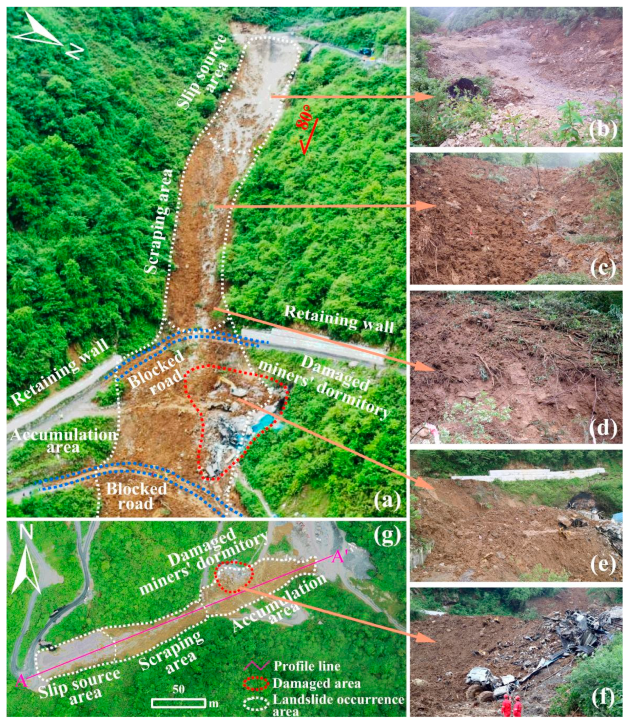
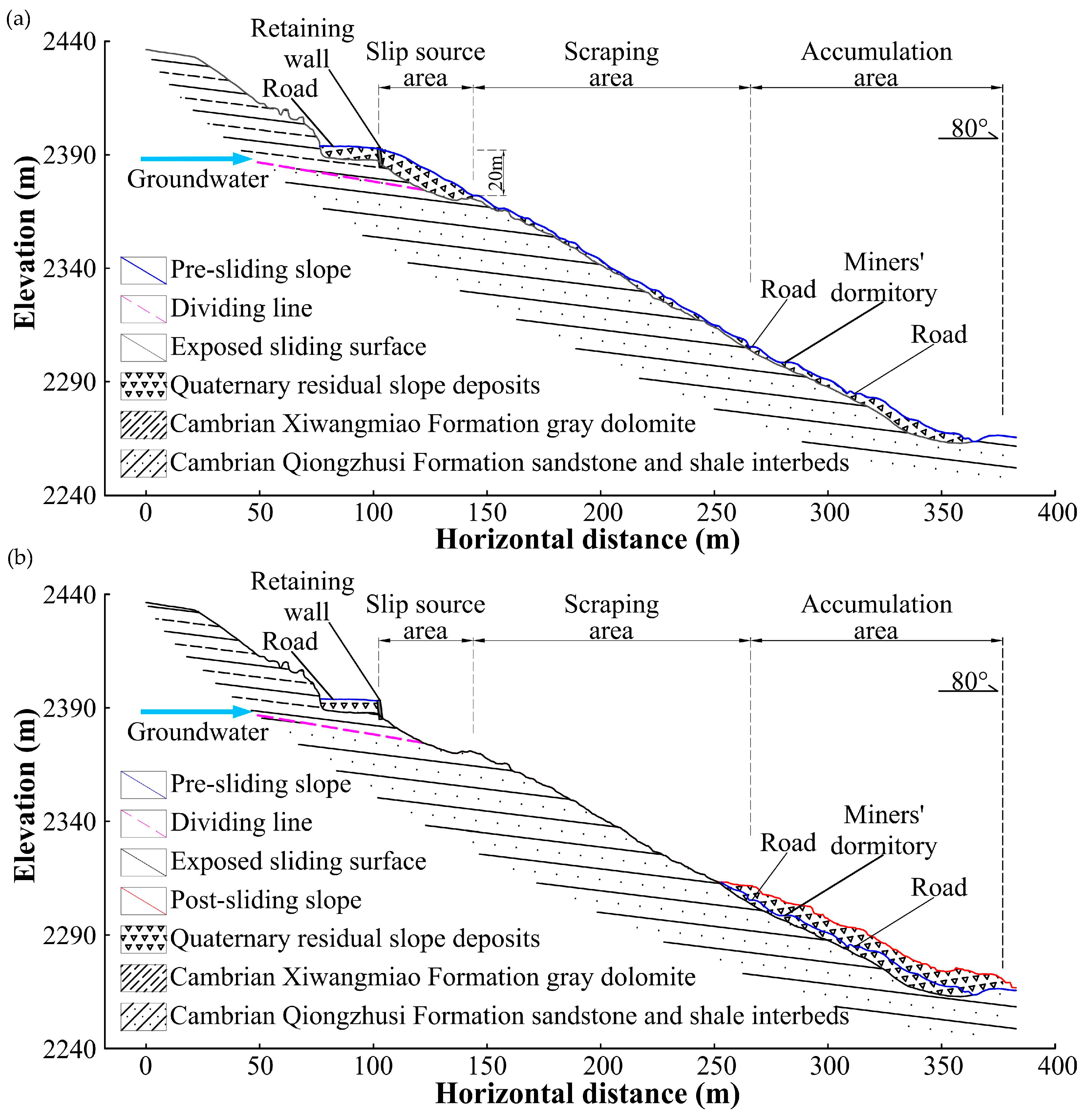
4.1. Basic Characteristics of the Landslide

The planform of the Yongsheng landslide resembles a long “tongue”, with a downslope length of 308 m, an average width of 36 m, and a sliding direction of 80°. Through the analysis of the topography, geomorphology, and depositional characteristics of the landslide area, we categorized it into the slip source area, the scarp area, and the accumulation area (as shown in Figure 5a). At the initiation of the landslide, approximately 1.3 × 10⁴ m³ of soil became destabilized due to continuous heavy rainfall and nearby human engineering activities. The soil subsequently fractured and disintegrated, rapidly sliding downslope from the slip source area (as shown in Figure 5b), scraping loose soil from the slope surface (Figure 5c,d), with the volume increasing to approximately 2 × 10⁴ m³. Part of the landslide body destroyed and buried the miners’ dormitory at the foot of the mountain, disrupted mining area roads, knocked down utility poles, causing a fire, and destroyed vehicles parked near the dormitory, resulting in approximately 3.1 × 10⁴ m³ of loose landslide debris (Figure 5e,f).

A cross-section A-A’ of the landslide was selected (Figure 5g), and a geological profile of the pre-landslide sliding surface was drawn (Figure 6a). Based on post-landslide field investigations and high-precision DEM obtained from UAV imagery, the post-landslide geological profile was drawn (Figure 6b). From the figures, it can be seen that the elevation at the rear edge is approximately 2397 m, and the lowest point of the front edge of the landslide surface is approximately 2277 m, with a relative height difference of 120 m. The slip source area of the landslide has a longitudinal length of 76 m, a height difference of 20 m, an average width of about 23 m, and an average thickness of 6 m. The scarp area has a longitudinal length of 96.4 m, an average width of about 17 m, and an average thickness of about 3 m. The accumulation area has a longitudinal length of 110.9 m, an average width of about 38 m, and an average thickness of about 6 m.

The sliding surface of the landslide is steep at the upper part and gentle at the lower part, forming a near-arc shape (as shown in Figure 7a). The slip source area of the landslide is located within a groove mid-slope on the mountain, the upper part of which consists of limestone from the Loushanguan Formation, characterized by well-developed rock joints and a downslope slope direction. At the rear edge of the landslide (viewed from top to bottom), a significant amount of residual abandoned slag is evident, comprising approximately 10% of the total volume of the collapsed mass (as shown in Figure 7b). Approximately 15 m to the right of the rear edge, there is a water diversion tunnel under construction, with an entrance width of 4 m and a height of 3 m (as shown in Figure 7c). According to the data, the construction length of the water diversion tunnel was approximately 57 m during the landslide. The abandoned slag generated during excavation was partially used for road construction, with the remaining portion deposited at the rear edge. On-site observations indicate significant seepage on the rear wall of the landslide, as shown in Figure 7d.

4.2. Characteristics of Pre-Landslide Deformation

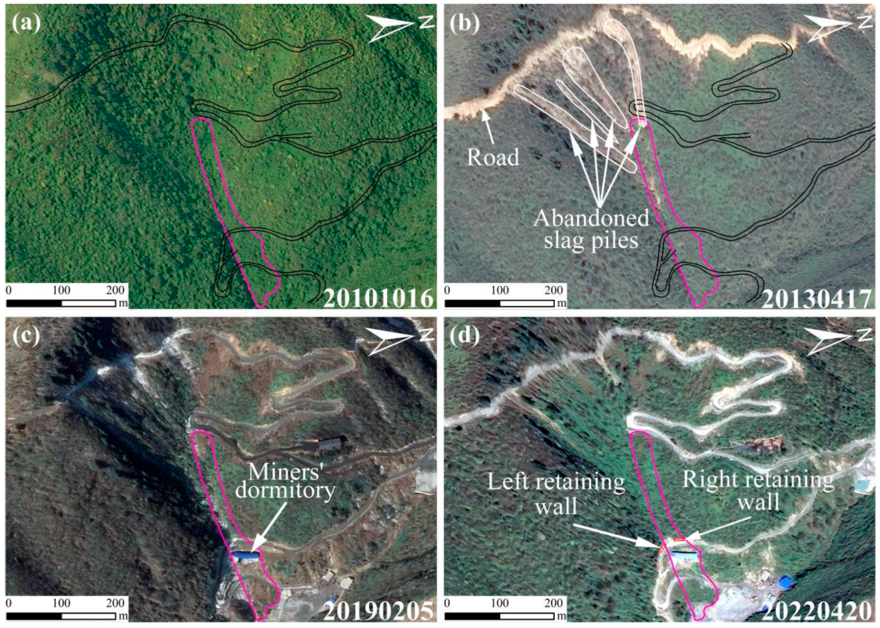
4.2.1. Analysis of Historical Imagery before Landslides

In the observation on 16 October 2010, no evident engineering activity was detected in the landslide area. The vegetation coverage of the gully watershed was approximately 92%, predominantly consisting of trees and shrubs (as shown in Figure 8a). By 17 April 2013, newly constructed roads were observed in the landslide area, with slope cuts during road construction altering the original landform. Simultaneously, abandoned slag was piled up in the catchment area within the gully at the top of the landslide area, and the image showed several long strips of white abandoned slag piles (as shown in Figure 8b). The observation on 5 February 2019 revealed evident human engineering activities in the landslide area, with accumulations in the slip source area and noticeable changes in the terrain height and slope within the gully. Additionally, a miners’ dormitory had been constructed at the bottom of the gully (as shown in Figure 8c). On 20 April 2022, two concrete retaining walls were constructed on the inner side of the road at the bottom of the gully, thereby widening the road foundation (as shown in Figure 8d). Compared to the observation image from 5 February 2019, no significant changes were detected in this area.

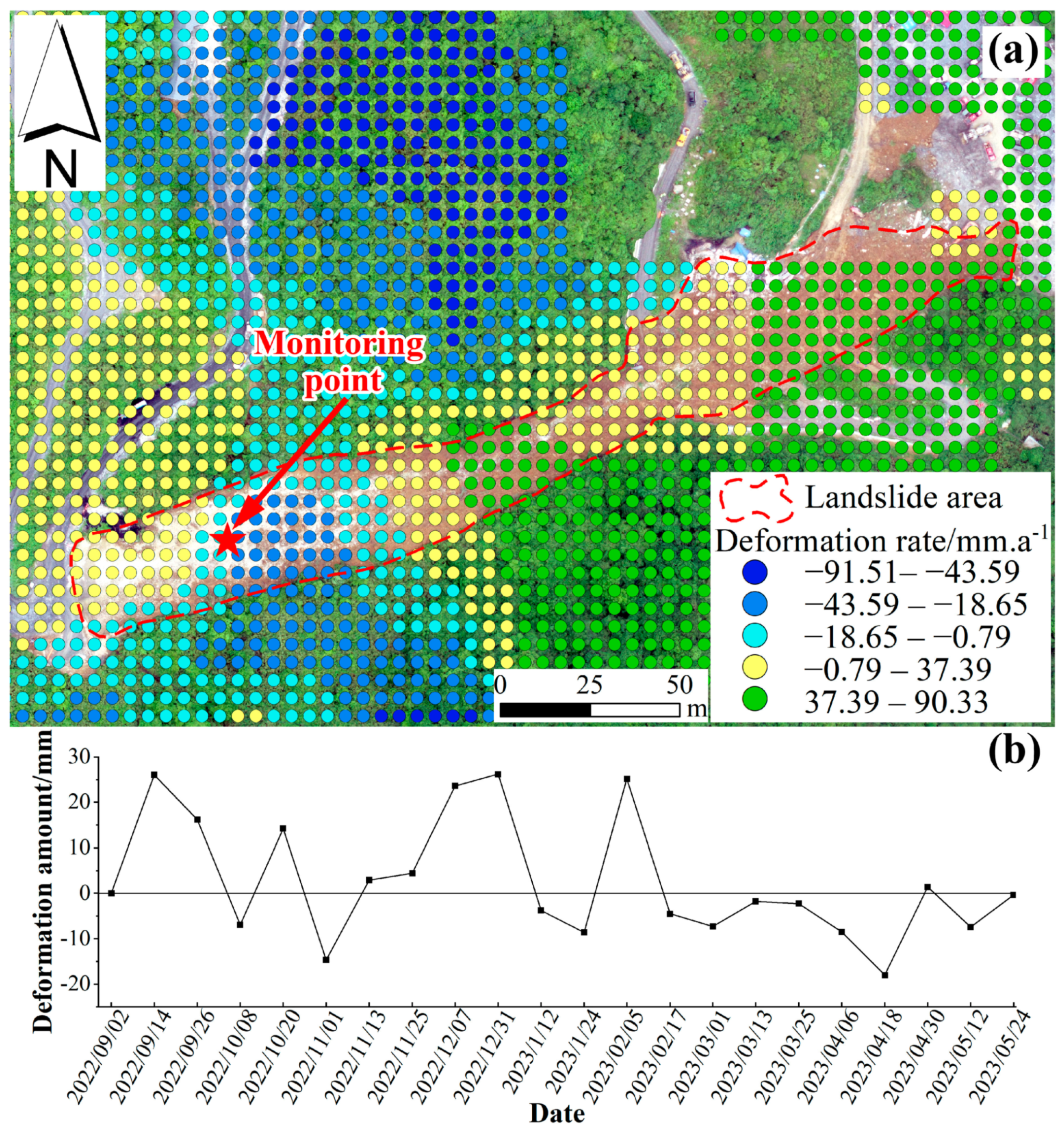
4.2.2. Analysis of Pre-Landslide Surface InSAR Deformation

Using the SBAS-InSAR method, 22 Sentinel radar satellite data scenes were analyzed from 2 September 2022 to 24 May 2023, generating a surface deformation rate map for the landslide area (Figure 9a). In the map, positive values indicate an uplift towards the satellite, while negative values indicate subsidence away from the satellite. The map reveals distinct deformation zones in the area prior to the landslide disaster. The section of the landslide source area near the road showed varying uplift rates (yellow areas), with an annual average deformation rate ranging from −0.79–37.39 mm/a during this period. The central and nearby regions of the landslide source area also showed varying rates of subsidence (cyan and dark blue areas), with a maximum deformation rate of −43.59 mm/a. Areas with deformation rates exceeding 0 mm/a were located in the central and front parts of the landslide body.

Given that InSAR technology encounters difficulties in capturing large displacements (on the meter scale) and in detecting displacements exceeding the millimeter scale, this paper focuses on analyzing the characteristics of subtle surface deformations of the Yongsheng landslide, concentrating on minor deformations detectable by this technology. Due to the varying rates of subsidence and uplift in the source area during the study period, a centrally located monitoring point in the landslide source area was selected to monitor the deformation process. The time-series map is based on an image from 2 September 2022, assuming a surface displacement of 0 mm at that time. During this period, the monitoring point exhibited multiple instances of uplift in the early stages and several instances of subsidence in the later stages, with displacement fluctuating between −20–30 mm (Figure 9b). This indicates that the slope body underwent long-term creep deformation prior to the occurrence of the Yongsheng landslide. The SBAS-InSAR results clearly demonstrate the presence of deformation in the slip source area prior to the landslide. Additionally, historical imagery revealed human engineering activities within the slip source area, suggesting that the accumulation of abandoned slag may have contributed to the landslide.

4.3. Kinematic Process of the Landslide

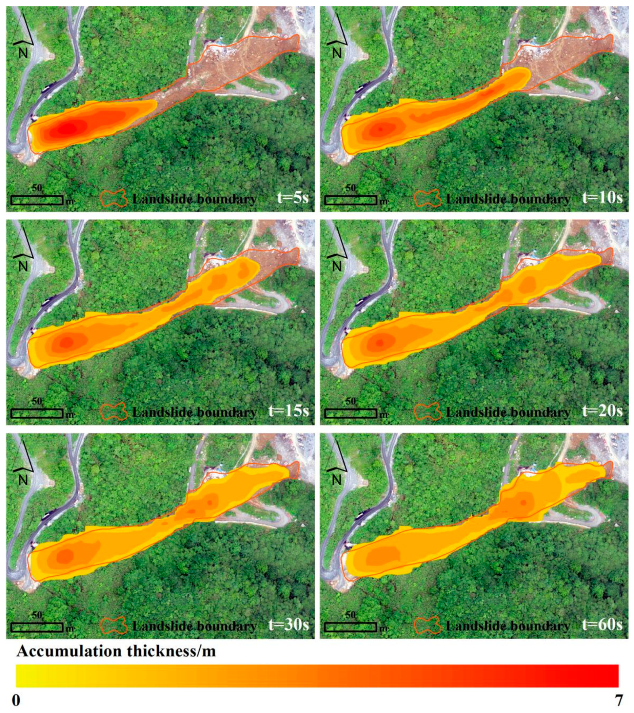
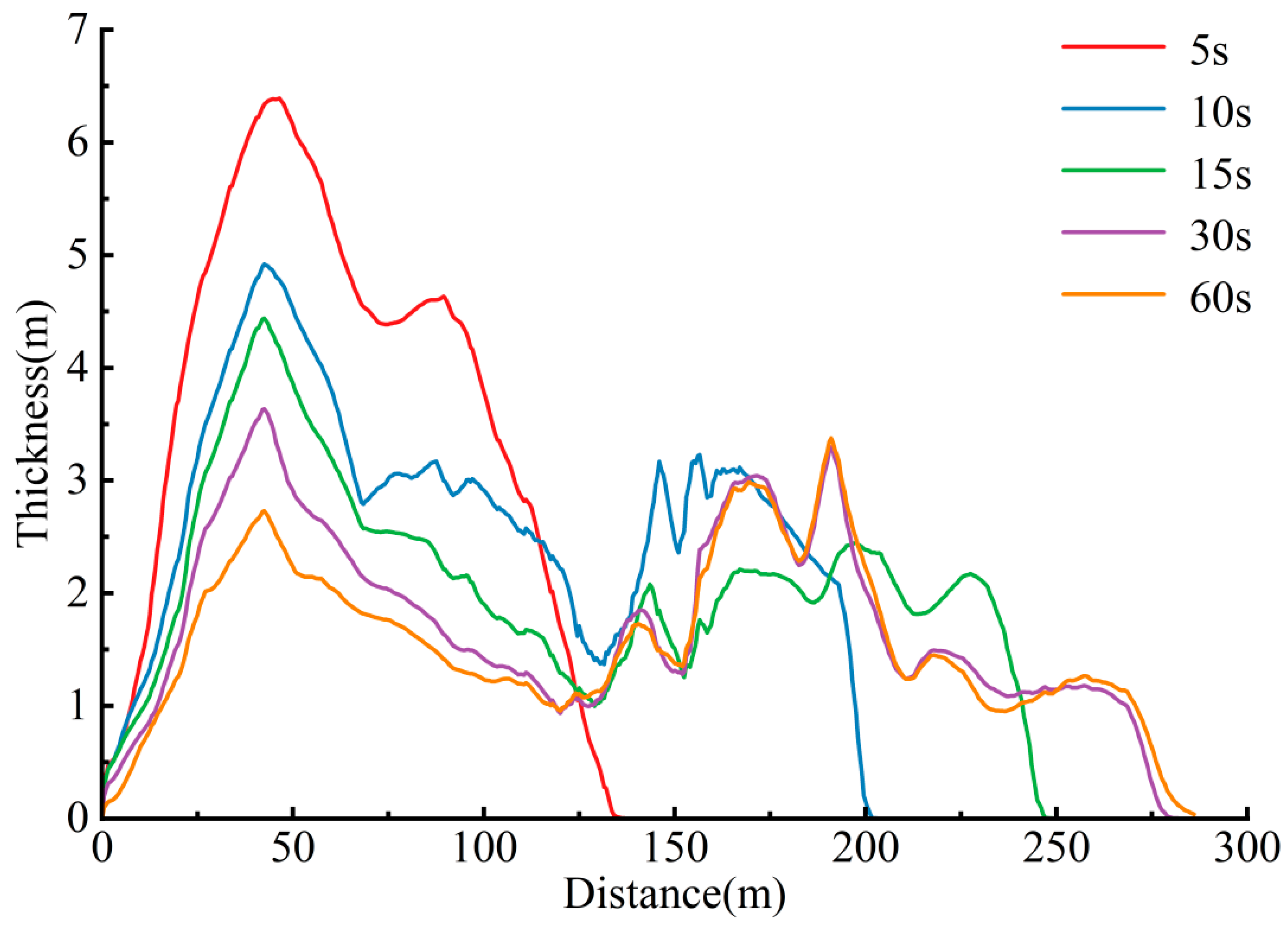
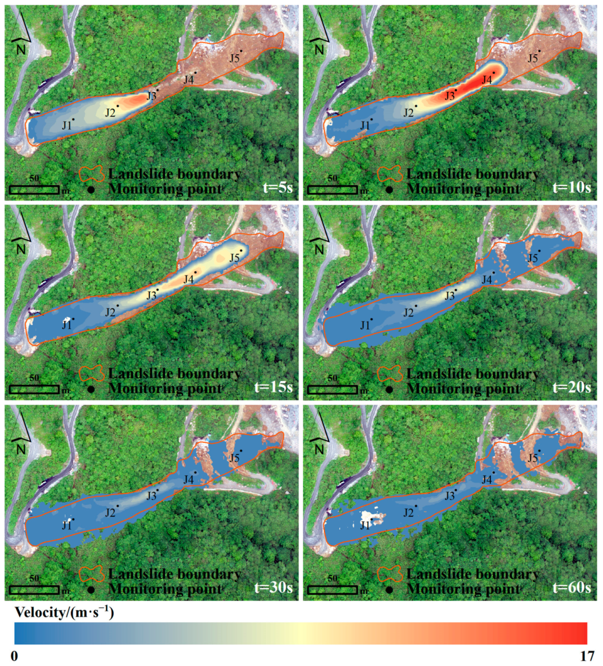
4.3.1. Analysis of Landslide Accumulation Range and Stages

The simulation results obtained using Massflow software are illustrated in Figure 10. Landslide movement forms at different time steps are depicted at 5 s intervals, with the entire landslide movement process lasting approximately 60 s. Due to the influence of terrain and landslide volume, the area and thickness of landslide deposition vary at different intervals. This landslide movement process is characterized by rapid initial movement followed by slower movement in later stages, with the maximum variation range of landslide deposition thickness being 0–7 m.

At t = 5 s, the front end of the landslide body moved forward by 42 m, which represents the period with the greatest longitudinal variation in deposition thickness. At t = 10 s, the landslide body accumulated and rushed down along the gully, with the front edge beginning to form deposits and causing damage to the miners’ dormitory. From 15–30 s, most of the landslide body had left the slip source area, and the expansion range of the front edge of the landslide body was still changing, moving forward by about 83 m. From 30–60 s, the forward movement of the landslide body stopped, with little overall change in deposition thickness except for a small area in the upper part of the slope. The maximum movement distance was about 286 m, eventually forming approximately 5.25 × 10³ m³ of loose landslide debris, with a deposition area of 3.54 × 10³ m².

Due to the strong mobility of the landslide, a certain degree of lateral diffusion was observed on its periphery. Considering source volume conservation, the numerically simulated deposition thickness is less than the actual deposition thickness.

The thickness of the accumulation body was extracted at five different times along section A-A’ (Figure 5g) to obtain the landslide accumulation thickness at different intervals, as shown in Figure 11.

Within 0–5 s, the debris at the rear edge of the landslide rapidly moved towards the front edge due to gravity, sliding 139 m, with a peak accumulation thickness of 6.4 m. Within 5–15 s, the accumulation thickness began to gradually decrease, with a large amount of debris at the rear edge still poised to slide, and the landslide slid to 249 m. Within 15–60 s, the thickness of the accumulation area stabilized, reaching its maximum extent at 60 s. The thickness at the rear edge of the landslide reached its minimum, while the front edge thickness remained almost unchanged, indicating that the overall movement of the landslide had ceased. The accumulation state at this point represents the final accumulation state.

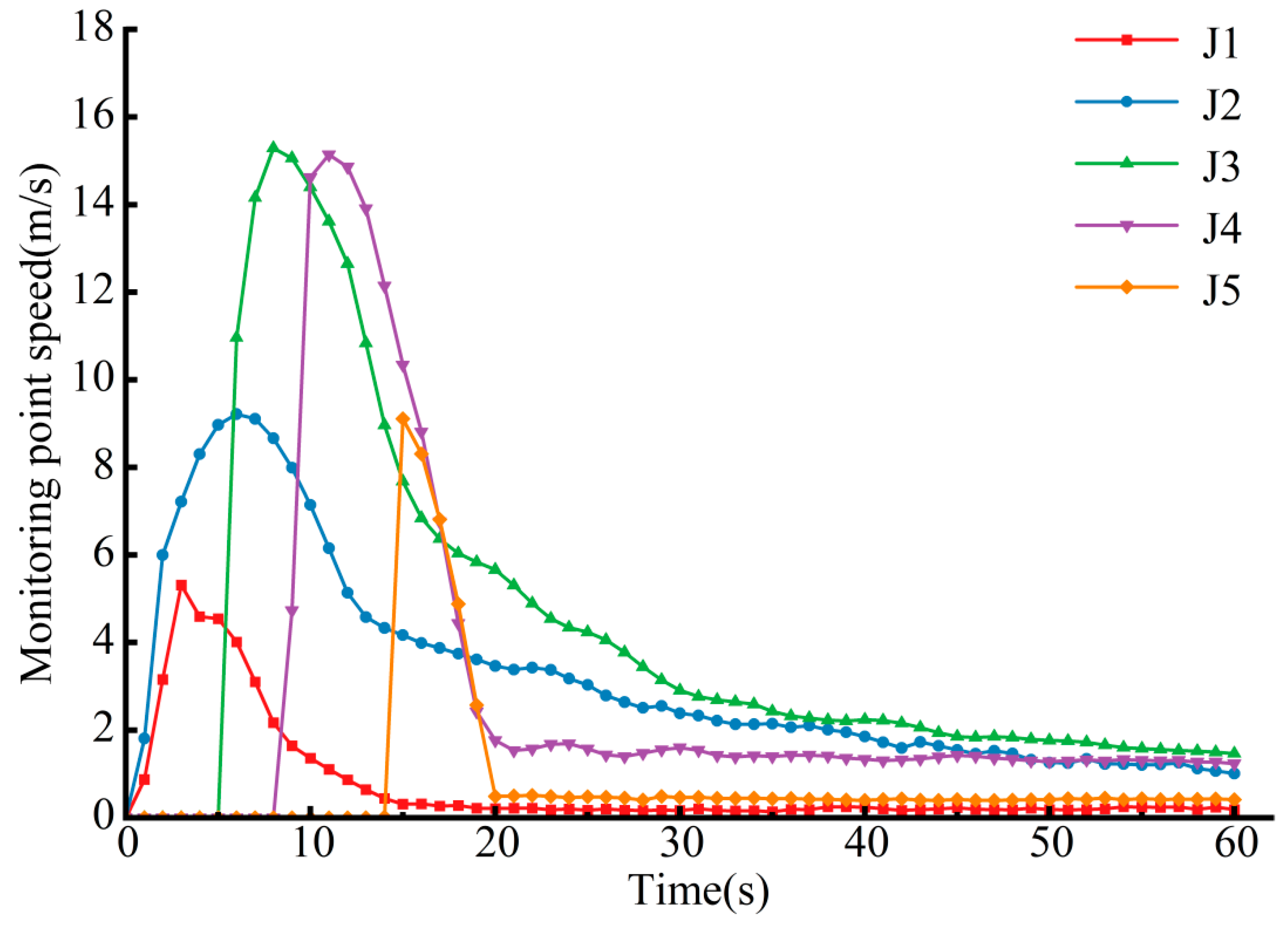
4.3.2. Analysis of Landslide Movement Velocity and Stages

The magnitude of landslide movement speed significantly affects the overall hazard intensity of the landslide. Figure 12 illustrates the speed distribution characteristics of the landslide body at different time intervals.

At t = 5 s, the landslide body was in an acceleration state, achieving a speed of 13.6 m/s. At t = 10 s, the speed reached a peak of 17 m/s, the highest value monitored during the entire movement of the landslide body, appearing in the frontal deposits and indicating that the kinetic energy of the frontal deposits was the greatest at this time. Between 15–60 s, as the range of the landslide body continued to expand forward, the speed at each node began to disperse and decrease. At t = 60 s, the main sliding zone has stopped, while localized small-scale sliding still occurred, and the speed at each node has decreased to below 2 m/s, indicating that most of the landslide bodies had stopped moving.

To further study the sliding characteristics of landslides at different stages, this study established monitoring points to observe changes in speed (Figure 13). J1 is located at the rear edge of the landslide, with a peak speed of 5.3 m/s. This area’s sliding body has high potential energy, and when passing through this point, the sliding body is still in the acceleration phase. J2 is located in the middle of the gully, where the speed is characterized by low acceleration and high velocity, reaching its peak speed at t = 6 s. The peak speed of J3 slightly lags behind those of the first two monitoring points, reaching 15.3 m/s at t = 8 s. J4 is located near the miners’ dormitory. The landslide impacts this area at a speed of 7.9 m/s at t = 9 s, and the speed continues to increase, reaching a peak speed of 15.1 m/s. After passing this point, the speed significantly decreases due to obstruction. J5 is located at the front edge of the landslide. After passing J4, the energy of the landslide decreases, resulting in a reduction in velocity.

The movement process of the Yongsheng landslide can be divided into three stages: the instability sliding stage, the sliding and scraping stage, and the deceleration and accumulation stage.

Instability Sliding Stage (0–5 s): During this stage, rain infiltrates the silty clay, causing it to absorb water and swell. This swelling reduces the gaps between the silty clay particles, thereby decreasing overall porosity. The altered soil structure becomes more compact, increasing pore water pressure. Due to the low permeability of silty clay, water movement within the soil is restricted, leading to the accumulation of pore water pressure. This increased pressure reduces the effective stress within the soil, thereby lowering its shear strength. Consequently, part of the soil may liquefy, resulting in landslide instability and sliding. The significant height difference in the landslide rapidly converts gravitational potential energy into kinetic energy, causing a gradual increase in movement speed.

Sliding and Scraping Stage (5–15 s): In this stage, the landslide body slides along the gully, entraining and continuously increasing the volume. The landslide body reaches its maximum speed as the kinetic energy increases.

Deceleration and Accumulation Stage (15–60 s): During the final stage, the landslide decelerates as it moves towards the leading edge area, where it begins to form an accumulation. The movement slows down significantly, and the debris starts to settle, marking the completion of the landslide’s motion.

5. Discussion

5.1. Causes of the Landslide

The landslide occurs in a groove area within the mid-mountain geomorphological zone, and the elevation at the ridge top at the groove’s rear is approximately 2600 m, with a relative height difference of 120 m between the front and rear edges. The slope of the landslide terrain ranges from 20°–30°, and the overall negative terrain facilitates the convergence of surface water, forming groundwater. Consequently, this process reduces the stability of the slope.

The maximum daily rainfall during the week preceding the landslide was 11.43 mm (Figure 3). An analysis of meteorological data from the past five years at the nearby Emei Mountain weather station indicates that the region typically experiences varied rainfall patterns, with an average annual precipitation of approximately 2005.6 mm. The occurrence of daily rainfall exceeding 10 mm is observed on average approximately 53 times per year. Therefore, although a daily rainfall of 10 mm may not be particularly uncommon, in conjunction with the preceding continuous rainfall, this amount of precipitation is sufficient to saturate the soil and create conditions conducive to a landslide. This precipitation likely generated infiltration-excess overland flow, which caused surface water to converge and seep into the gray dolomite of the Lower Cambrian Series at the top of the instability initiation zone, forming groundwater. We measured the flow using a volumetric flow meter that operates by continuously filling and emptying a standard small volume, with a recorded outflow of approximately 86 m³/d at the site. Both rainfall and groundwater collectively provided the dynamic conditions necessary for the collapse. Many small landslides typically occur when rainfall intensity increases or approaches its peak [33]. For instance, during the Yongsheng landslide, continuous heavy rainfall occurred in the month preceding the event. Notably, the two largest rainfall events occurred 18 and 28 days before the landslide, respectively. During the persistent rainfall, water infiltrated through cracks and structural planes, gradually accumulating as groundwater. With the increase in groundwater, both dynamic and static water pressures increased, leading to a reduction in the strength of the saturated soil and rock. This reduction in strength can trigger the redistribution and accumulation of stress, causing damage to the rock structure and eventually resulting in deformation and the occurrence of a landslide. The variation in the timing of landslide occurrences is attributed to the differential responses of various soil and rock types to rainfall infiltration and pore water pressure accumulation. In large-scale landslide events, there is typically a lag between the peak rainfall intensity and the occurrence of the landslide [34,35], reflecting the time required for rainwater to infiltrate into the deeper layers of the soil and rock. Unlike sudden landslides triggered directly by heavy rainfall [36], the Yongsheng landslide resulted from the cumulative effects of prior rainfall events. This suggests that when the rainfall intensity reaches a threshold, infiltration can rapidly induce changes in pore water pressure, precipitating landslides. Therefore, continuous heavy rainfall is a triggering factor in this landslide event.

Prior to the occurrence of the landslide, the area experienced extensive human engineering activities, including road construction, mining operations, and water diversion tunnel construction. These activities may have affected the stability of the natural slopes. Through on-site investigation and Google Earth historical images (Figure 8), it is evident that since 2012, the construction and maintenance of mine roads have produced approximately 900 m³ of abandoned slag. However, this abandoned slag was not promptly transported to designated locations but instead accumulated at the top of the slope instability initiation zone, thereby exerting a loading effect on the slope’s stability. Since 23 May 2023, approximately 400 m³ of additional abandoned slag was generated due to the construction of a water diversion tunnel on the right side of the landslide’s rear edge. This increased the total abandoned slag at the rear edge to approximately 1300 m³, causing the slope to approach a critical state of stability. At the same time, an analysis of pre-landslide surface deformation using SBAS-InSAR technology (Figure 9) revealed an uplift in the rear edge of the landslide. This uplift was caused by the accumulation of abandoned slag, while other parts of the rear edge exhibited subsidence at varying rates. The data is consistent with actual conditions, indicating that the accumulation of abandoned slag was a predisposing factor in the occurrence of this landslide.

5.2. Simulation Accuracy Analysis

The elevation difference results before and after the landslide can intuitively reflect the distribution of source material accumulation in various parts of the landslide. Regarding the accuracy of numerical simulations, the more the simulated accumulation is distributed outside the landslide boundary, the lower its accuracy; conversely, it indicates a higher accuracy of the numerical simulation. To quantitatively analyze the accuracy of numerical simulations, as shown in

Table 3. Statistics of numerical simulation accuracy parameters.

Data Type	$\mathit{L}$/m	${\mathit{S}}_{\mathit{i}}$/m2	${\mathit{S}}_{\mathit{b}}$/m2	$\mathit{S}$/m2	$\mathit{\eta }$
Real landslide body	284	7550	/	7550	100
Simulated landslide body	286	7011	1033	8044	79.2

, by statistically analyzing the simulated landslide displacement L, the area within the landslide boundary $S_i$, the area outside the landslide boundary $S_b$, the total landslide area $S$, and the actual landslide accumulation range $S_0$, the following formula for the accuracy $\eta$ of the Massflow numerical simulation is proposed [37]:

$$\eta ={\displaystyle \frac{S_i-S_b}{S_0}}$$

(4)

The accuracy η obtained from the simulated landslide event is lower than that of the actual landslide. Analysis indicates that, after instability, the motion process of the Yongsheng Landslide resembles that of a debris flow landslide. After the slope experiences instability and failure, it gradually fractures and disintegrates during movement, exhibiting fluid-like motion characteristics as it slides toward the gully mouth. If the slopes on both sides are relatively gentle and unconstrained, the landslide tends to flow freely on the surface. Due to the high mobility, the slip source and accumulation areas exhibit a certain degree of lateral spread along the direction of the landslide body, increasing the area outside the landslide boundary and thereby reducing the simulation accuracy η. Analysis of the simulation results indicates that the maximum erosion depth near the slip source area is consistent with the actual depth. It can be concluded that the numerical simulation results from Massflow are generally consistent with the actual accumulation situation.

Moreover, this study does not take into account the effects of erosion during the landslide process. In a real-world scenario, the landslide mass can also incorporate surrounding loose soil and rock particles, further increasing its volume. The substantial increase in landslide volume poses major challenges for numerical simulations. Although existing numerical codes like Delft3D [38] and Telemac [39] can calculate erosion, they still face numerous difficulties in simulating substantial changes in landslide volume. First, accurately capturing the erosion and incorporation processes during landslides requires precise data on surface material properties and dynamics. Secondly, balancing computational efficiency and accuracy is a key issue, as high-precision numerical calculations can significantly increase computation time. Additionally, several parameters in numerical models, such as erosion rate and incorporation coefficient, need to be calibrated and validated with field observation data to ensure the reliability of the simulation results. Future research should focus on enhancing the physical basis of numerical models, developing a deeper understanding of the specific mechanisms of erosion and incorporation during landslides through more field experiments and observations, and incorporating these mechanisms into numerical models. By improving computational algorithms and developing more efficient computational methods, both computational efficiency and simulation accuracy can be enhanced. Utilizing big data and machine learning technologies to extract patterns from a large number of landslide events and further optimize numerical model parameters can also be beneficial. These improvements will help enhance the accuracy of landslide disaster prediction and risk assessment.

6. Conclusions

This study conducted a comprehensive analysis of the developmental characteristics of the Yongsheng landslide through detailed field investigations in conjunction with factors such as topography, rainfall, and human engineering activities. By utilizing historical landslide imagery, UAV aerial photography, and InSAR deformation analysis over different periods, high-resolution imagery and surface deformation data were obtained for various time periods, providing substantial data support for the study of landslide instability characteristics. Based on this, a Massflow numerical model was developed to simulate the dynamic process of the entire landslide. The simulation results indicate that the landslide ceased movement after sliding for 60 s, covering a distance of approximately 286 m. The maximum accumulation thickness reached 7 m, and the maximum sliding speed was 17 m/s, ultimately resulting in approximately 5.25 × 10³ m³ of loose landslide debris. Compared to actual observations, the simulation results reflect the landslide movement process to a considerable extent, exhibiting a high degree of consistency in movement characteristics and accumulation morphology. Through the comprehensive application of multi-source data, this study provides a systematic framework for landslide analysis and, for the first time, quantitatively analyzes the movement patterns of the Yongsheng landslide using the Massflow model. This offers a scientific basis for the optimization of landslide disaster identification, monitoring, and early warning systems.

References

1. Zhao, C.; Lu, Z. Remote Sensing of Landslides—A Review. Remote Sens. 2018, 10, 279. [Google Scholar] [CrossRef]
2. Dai, F.; Lee, C.; Wang, S. Characterization of rainfall-induced landslides. Int. J. Remote Sens. 2003, 24, 4817–4834. [Google Scholar] [CrossRef]
3. Fan, L.; Lehmann, P.; Mcardell, B.; Or, D. Linking rainfall-induced landslides with debris flows runout patterns towards catchment scale hazard assessment. Geomorphology 2017, 280, 1–15. [Google Scholar] [CrossRef]
4. Li, Y.; Ma, C.; Wang, Y. Landslides and debris flows caused by an extreme rainstorm on 21 July 2012 in mountains near Beijing, China. Bull. Eng. Geol. Environ. 2019, 78, 1265–1280. [Google Scholar] [CrossRef]
5. Yin, Y.; Zheng, W.; Li, X.; Sun, P.; Li, B. Catastrophic landslides associated with the M8. 0 Wenchuan earthquake. Bull. Eng. Geol. Environ. 2011, 70, 15–32. [Google Scholar] [CrossRef]
6. Shrestha, S.; Kang, T. Assessment of seismically-induced landslide susceptibility after the 2015 Gorkha earthquake, Nepal. Bull. Eng. Geol. Environ. 2019, 78, 1829–1842. [Google Scholar] [CrossRef]
7. Lin, C.; Chang, W.; Liu, S.; Tsai, T.; Lee, S.; Tsang, Y.; Shieh, C.; Tseng, C. Landslides triggered by the 7 August 2009 Typhoon Morakot in southern Taiwan. Eng. Geol. 2011, 123, 3–12. [Google Scholar] [CrossRef]
8. Bhardwaj, A.; Wasson, R.; Ziegler, A.; Ziegler, A.; Chow, W.; Sundriyal, Y. Characteristics of rain-induced landslides in the Indian Himalaya: A case study of the Mandakini Catchment during the 2013 flood. Geomorphology 2019, 330, 100–115. [Google Scholar] [CrossRef]
9. Bezak, N.; Jež, J.; Sodnik, J.; Jemec, A.; Mikoš, M. An extreme May 2018 debris flood case study in northern Slovenia: Analysis, modelling, and mitigation. Landslides 2020, 17, 2373–2383. [Google Scholar] [CrossRef]
10. Kotlyakov, V.; Rototaeva, O.; Nosenko, G. The September 2002 Kolka glacier catastrophe in North Ossetia, Russian Federation: Evidence and analysis. Mt. Res. Dev. 2004, 24, 78–83. [Google Scholar] [CrossRef]
11. Ma, P.; Peng, J.; Wang, Q.; Zhuang, J.; Zhang, F. The mechanisms of a loess landslide triggered by diversion-based irrigation: A case study of the South Jingyang Platform, China. Bull. Eng. Geol. Environ. 2019, 78, 4945–4963. [Google Scholar] [CrossRef]
12. Cui, Y.; Xu, C.; Xu, S.; Chai, S.; Fu, G.; Bao, P. Small-scale catastrophic landslides in loess areas of China: An example of the March 15, 2019, Zaoling landslide in Shanxi Province. Landslides 2020, 17, 669–676. [Google Scholar] [CrossRef]
13. Zhang, F.; Liu, G.; Chen, W.; Liang, S.; Chen, R.; Han, W. Human-induced landslide on a high cut slope: A case of repeated failures due to multi-excavation. J. Rock Mech. Geotech. Eng. 2012, 4, 367–374. [Google Scholar] [CrossRef]
14. Zhuang, Y.; Xing, A.; Jiang, Y.; Sun, Q.; Yan, J.; Zhang, Y. Typhoon, rainfall and trees jointly cause landslides in coastal regions. Eng. Geol. 2022, 298, 106561. [Google Scholar] [CrossRef]
15. Cui, Y.; Hu, J.; Xu, C.; Zheng, J.; Wei, J. A catastrophic natural disaster chain of typhoon-rainstorm-landslide-barrier lake-flooding in Zhejiang Province, China. J. Mt. Sci. 2021, 18, 2108–2119. [Google Scholar] [CrossRef]
16. Yin, Y. Recent catastrophic landslides and mitigation in China. J. Rock Mech. Geotech. Eng. 2011, 3, 10–18. [Google Scholar] [CrossRef]
17. Lin, Q.; Wang, Y. Spatial and temporal analysis of a fatal landslide inventory in China from 1950 to 2016. Landslides 2018, 15, 2357–2372. [Google Scholar] [CrossRef]
18. Poisel, R.; Preh, A.; Hungr, O. Run out of landslides–continuum mechanics versus discontinuum mechanics models. Geomech. Tunnelbau 2008, 1, 358–366. [Google Scholar] [CrossRef]
19. Roslan, R.; Omar, R.; Putri, R.; Wahab, W.; Baharuddin, I.; Jaafar, R. Slope stability analysis using Universal Distinct Element Code (UDEC) method. IOP Conf. Ser. Earth Environ. Sci. 2020, 451, 012081. [Google Scholar] [CrossRef]
20. Filice, F.; Pezzo, A.; Lollino, P.; Perrotti, M.; Ietto, F. Multi-approach for the assessment of rock slope stability using in-field and UAV investigations. Bull. Eng. Geol. Environ. 2022, 81, 502. [Google Scholar] [CrossRef]
21. Schilirò, L.; Massaro, L.; Forte, G.; Santo, A.; Tommasi, P. Analysis of Earthquake-Triggered Landslides through an Integrated Unmanned Aerial Vehicle-Based Approach: A Case Study from Central Italy. Remote Sens. 2024, 16, 93. [Google Scholar] [CrossRef]
22. Niethammer, U.; James, M.; Rothmund, S.; Travelletti, J.; Joswig, M. UAV-based remote sensing of the Super-Sauze landslide: Evaluation and results. Eng. Geol. 2012, 128, 2–11. [Google Scholar] [CrossRef]
23. Massaro, L.; Forte, G.; De Falco, M.; Rauseo, F.; Santo, A. Rockfall source identification and trajectory analysis from UAV-based data in volcano-tectonic areas: A case study from Ischia Island, Southern Italy. Bull. Eng. Geol. Environ. 2024, 83, 75. [Google Scholar] [CrossRef]
24. Ouyang, C.; Zhou, K.; Xu, Q.; Yin, J.; Peng, D.; Wang, D.; Li, W. Dynamic analysis and numerical modeling of the 2015 catastrophic landslide of the construction waste landfill at Guangming, Shenzhen, China. Landslides 2017, 14, 705–718. [Google Scholar] [CrossRef]
25. Scaringi, G.; Fan, X.; Xu, Q.; Liu, C.; Ouyang, C.; Domènech, G.; Yang, F.; Dai, L. Some considerations on the use of numerical methods to simulate past landslides and possible new failures: The case of the recent Xinmo landslide (Sichuan, China). Landslides 2018, 15, 1359–1375. [Google Scholar] [CrossRef]
26. Fan, X.; Yang, F.; Siva, S.; Xu, Q.; Feng, Z.; Mavrouli, O.; Peng, M.; Ouyang, C.; Jansen, J.; Huang, R. Prediction of a multi-hazard chain by an integrated numerical simulation approach: The Baige landslide, Jinsha River, China. Landslides 2020, 17, 147–164. [Google Scholar] [CrossRef]
27. Ouyang, C.; He, S.; Xu, Q.; Luo, Y.; Zhang, W. A MacCormack-TVD finite difference method to simulate the mass flow in mountainous terrain with variable computational domain. Comput. Geosci. 2013, 52, 1–10. [Google Scholar] [CrossRef]
28. Zhao, C.; Kang, Y.; Zhang, Q.; Lu, Z.; Li, B. Landslide Identification and Monitoring along the Jinsha River Catchment (Wudongde Reservoir Area), China, Using the InSAR Method. Remote Sens. 2018, 10, 993. [Google Scholar] [CrossRef]
29. Ouyang, C.; He, S.; Xu, Q. MacCormack-TVD finite difference solution for dam break hydraulics over erodible sediment beds. J. Hydraul. Eng. 2015, 141, 06014026. [Google Scholar] [CrossRef]
30. Ching, J.; Schweckendiek, T. State-of-the-art review of inherent variability and uncertainty in geotechnical properties and models. ISSMGE Tech. Comm. 2021, 304, 219. Available online: http://140.112.12.21/issmge/2021/SOA_Review_on_geotechnical_property_variablity_and_model_uncertainty.pdf (accessed on 2 August 2024).
31. Chu, H.; Sun, C.; Zhang, X.; Li, C. Research on engineering geology characteristics of Wangshan-Zhuakousi landslide in sliding zone in Emeishan city. Chin. J. Geol. Hazard Control 2017, 28, 48–52. [Google Scholar] [CrossRef]
32. Chen, X.; Zhao, Z.; Wei, J.; Xu, C. Numerical study of Mabian landslide kinematics and impact intensity. Coal Geol. Explor. 2021, 49, 234–241. [Google Scholar] [CrossRef]
33. Godt, J.; Baum, R.; Chleborad, A. Rainfall characteristics for shallow landsliding in Seattle, Washington, USA. Earth Surf. Process. Landf. J. Br. Geomorphol. Res. Group 2006, 31, 97–110. [Google Scholar] [CrossRef]
34. Chigira, M. September 2005 rain-induced catastrophic rockslides on slopes affected by deep-seated gravitational deformations, Kyushu, southern Japan. Eng. Geol. 2009, 108, 1–15. [Google Scholar] [CrossRef]
35. Evans, S.; Guthrie, R.; Roberts, N.; Bishop, N. The disastrous 17 February 2006 rockslide-debris avalanche on Leyte Island, Philippines: A catastrophic landslide in tropical mountain terrain. Nat. Hazards Earth Syst. Sci. 2007, 7, 89–101. [Google Scholar] [CrossRef]
36. De Falco, M.; Forte, G.; Marino, E.; Massaro, L.; Santo, A. UAV and field survey observations on the November 26th 2022 Celario flowslide, Ischia Island (Southern Italy). J. Maps 2023, 19, 2261484. [Google Scholar] [CrossRef]
37. Zhou, Q.; Xu, Q.; Zhou, X.; Zhao, K.; Xiu, D.; Peng, D. Research on the predicting hazard range of abrupt loess landslide—A case study of jj6 # landslide in Heifangtai tableland. J. Catastrophol. 2020, 35, 216–221. [Google Scholar] [CrossRef]
38. Elias, E.; Walstra, D.; Roelvink, J.; Stive, M.; Klein, M. Hydrodynamic validation of Delft3D with field measurements at Egmond. Coast. Eng. 2001, 2000, 2714–2727. [Google Scholar] [CrossRef]
39. Villaret, C.; Hervouet, J.; Kopmann, R.; Merkel, U.; Davies, A. Morphodynamic modeling using the Telemac finite-element system. Comput. Geosci. 2013, 53, 105–113. [Google Scholar] [CrossRef]
Figure 1. Geographical location map of the study area.
Remotesensing 16 03324 g001
Figure 2. Geological map of the study area.
Remotesensing 16 03324 g002
Figure 3. Daily rainfall and cumulative rainfall data for 1 May–4 June 2023 from the Emei Mountain meteorological station.
Remotesensing 16 03324 g003
Figure 4. Flowchart of research methodology.
Remotesensing 16 03324 g004
Figure 5. Landslide Characteristics: (a) Panoramic view of the Yongsheng landslide (modified from a picture from www.news.cn); (b) on-site photo of the slip source area; (c) on-site photo of the scraping area; (d) scraped landslide body; (e) on-site photo of the damaged miners’ dormitory; (f) destroyed vehicles; and (g) overhead view of the Yongsheng landslide (photographed by UAV).
Remotesensing 16 03324 g005
Figure 6. Geological profile A-A’: (a) Pre-landslide profile, and (b) post-landslide profile.
Remotesensing 16 03324 g006
Figure 7. Characterization of the trailing edge of the landslide: (a) Overview of the trailing edge of the landslide; (b) exposed sliding surface; (c) water diversion tunnel on the right side of the rear edge; and (d) seepage area on the trailing edge wall.
Remotesensing 16 03324 g007
Figure 8. Historical imagery of the landslide area: (a) Google Earth imagery for 16 October 2010; (b) Google Earth imagery for 17 April 2013; (c) Google Earth imagery for 5 February 2019; and (d) Google Earth imagery for 20 April 2022.
Remotesensing 16 03324 g008
Figure 9. Landslide radar satellite imagery time-series differential results: (a) Time-series difference map of surface displacement satellite data; and (b) deformation curve of the monitoring point.
Remotesensing 16 03324 g009
Figure 10. Numerical simulation of landslide accumulation extent at different moments.
Remotesensing 16 03324 g010
Figure 11. Schematic diagram of longitudinal accumulation thickness of landslides at different moments in time.
Remotesensing 16 03324 g011
Figure 12. Numerical simulation of landslide motion velocity at different times.
Remotesensing 16 03324 g012
Figure 13. Velocity variation of monitoring points at different times.
Remotesensing 16 03324 g013