Enhancing Alfalfa Biomass Prediction: An Innovative Framework Using Remote Sensing Data

Abstract

Estimating pasture biomass has emerged as a promising avenue to assist farmers in identifying the best cutting times for maximizing biomass yield using satellite data. This study aims to develop an innovative framework integrating field and satellite data to estimate aboveground biomass in alfalfa (Medicago sativa L.) at farm scale. For this purpose, samples were collected throughout the 2022 growing season on different mowing dates at three fields in Kansas, USA. The satellite data employed comprised four sources: Sentinel-2, PlanetScope, Planet Fusion, and Biomass Proxy. A grid of hyperparameters was created to establish different combinations and select the best coefficients. The permutation feature importance technique revealed that the Planet’s PlanetScope near-infrared (NIR) band and the Biomass Proxy product were the predictive features with the highest contribution to the biomass prediction model’s. A Bayesian Additive Regression Tree (BART) was applied to explore its ability to build a predictive model. Its performance was assessed via statistical metrics (r²: 0.61; RMSE: 0.29 kg.m⁻²). Additionally, uncertainty quantifications were proposed with this framework to assess the range of error in the predictions. In conclusion, this integration in a nonparametric approach achieved a useful predicting tool with the potential to optimize farmers’ management decisions.

1. Introduction

Alfalfa (Medicago sativa L.) is a perennial forage legume widely cultivated in arid and semi-arid regions. This forage crop gained popularity among farmers in recent decades due to its agronomic and nutritive value [1,2]. Alfalfa is highly productive, nutrient-rich (with a protein content ranging 15–22%), capable of fixing nitrogen, and adaptable to diverse environmental conditions [3,4]. Alfalfa is commonly cultivated in a four-year rotation, not only because it enhances nitrogen levels for subsequent crops but also because younger stands yield higher yields than older stands [5,6]. Optimal production is contingent upon the implementation of an array of management practices, including irrigation, fertilization, weed control, and disease management. When these practices are properly executed, as a perennial crop, alfalfa fields can be harvested multiple times within a single growing season, during the same growing season, and across years (e.g., for approximately 3–4 times), contingent upon the prevailing climatic and soil conditions [7,8]. This characteristic contributes to a production system that is both sustainable and economically viable [9]. Furthermore, alfalfa has multiple uses, including hay, silage, and pasture. Additionally, it serves as a source for by-products utilized in biofuel production, pharmaceutical compounds, enzymes, and industrial proteins [10]. Despite all these favorable characteristics, inadequate planning in determining mowing or grazing times can lead to low and inconsistent forage production, posing a challenge to meeting the yield and nutritional requirements for livestock [11].

Addressing the challenge of inconsistent forage production, satellite remote sensing-based models have emerged as a promising solution for estimating forage quantity and nutritive value [12,13]. The scientific literature on remote sensing for alfalfa is scarce, focusing on terrestrial and satellite platforms. Biomass regression models frequently compare data from disparate sources rather than integrating them. For example, Song et al. (2021) [14] showed that combining satellite data like Sentinel-2 and MODIS enhances temporal resolution, improving alfalfa harvest monitoring. Similarly, Wang et al. (2020) [15] found that integrating data from multiple sources is more effective for wheat monitoring than using a single satellite source. Consequently, an evaluation was conducted of the efficacy of different spectral bands from various sources in the estimation of biomass. Remote sensing and field data combined with advanced algorithms, such as regression trees (RT), support vector machine (SVM), and extreme gradient boosting models (XGBoost), have been successfully employed to predict biomass and quality characteristics in alfalfa and other crops [16,17,18]. Additionally, these models have also been instrumental in leaf area index [19] and phenotypic determinations [20]. These tools already play a significant role in pastoral decision-making and the improvement of management strategies. However, estimating biomass via remote sensing remains challenging, requiring multi-source data, features, and algorithm selection to enhance biomass estimation performance [21]. Among recent approaches, the Bayesian Additive Regression Trees (BART) algorithm has experienced rapid development and gained widespread popularity in various applications [22]. The incorporation of BART into the analysis was based on the observation that most preceding studies have concentrated on models that yield point estimates but yet fail to provide confidence intervals for biomass predictions [12,23]. A major issue with these approaches is the lack of uncertainty quantification, leading to limited or inaccurate interpretations. This is the case of Linear and generalized linear models (GLMs) are useful for summarizing linear relationships between predictors and responses. However, they fall short when dealing with complex nonlinear patterns. In such cases, nonparametric regressions are a better alternative, as they allow the relationship to be determined directly by the data [24,25]. BART represents a non-parametric ensemble regression tree model constructed by amalgamating a collective assembly of weakly performing decision trees [26]. Furthermore, the Bayesian framework allows the consideration of nonlinear patterns between dependent variables and predictors and the assessment of the uncertainty in the prediction, improving the ability of current models to capture uncertainty and provide sensitivity analysis [27]. From a productive standpoint, it is essential to consider the uncertainties of the predictions during the decision-making process and to change from static to dynamic decision-making [28].

Following this rationale, this study employed field and satellite data to develop an innovative framework to estimate aboveground biomass in alfalfa at the on-farm scale. Specific objectives were to (i) determine the best spectral bands to build an alfalfa biomass predictive model and (ii) explore the capability of BART regression models to predict alfalfa biomass by assessing its performance.

2. Materials and Methods

2.1. Study Area

The study was conducted at the farm level in three fields in Wichita, Kansas, United States (Figure 1) during the 2022 summer season (May to August). The area is described as flat plains at 1050 m above sea level [29] with a semi-humid and semi-arid climate zone with an annual mean temperature of 14 °C. Two fields were under dryland conditions (Fields 2 and 3, Figure 1C,D), while the remaining was under irrigated conditions (Field 1, Figure 1B).

Table 1. Mean, minimum, and maximum temperature (°C) and cumulative precipitations (mm) from May 1st to September 30st. Obtained from Mesonet (Station Mount Hope 3NE GDM).

Weather Variable	Value
Mean temperature (°C)	24
Minimum temperature (°C)	3.7
Maximum temperature (°C)	41
Cumulative precipitation (mm)	384

describes the temperature and precipitations for the studied season. The lowest and highest temperatures recorded during the study were −22 °C and 41 °C, respectively [30]. May was the month with the highest precipitation, with a cumulative value of 208 mm.

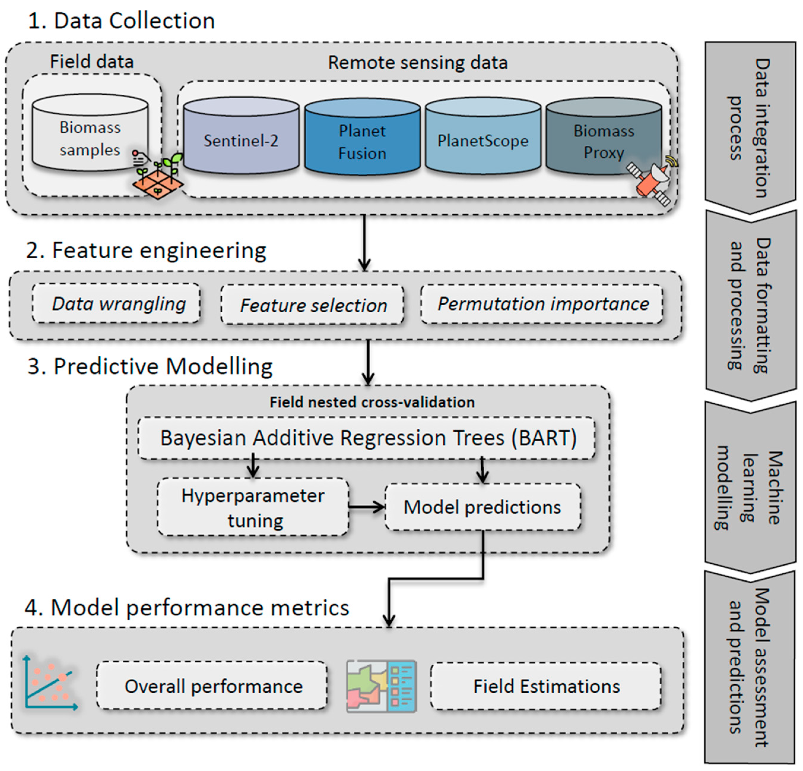
2.2. Framework Development

Figure 2 presents the framework followed in this study, showcasing four main stages or levels: 1. Data collection, 2. Feature Engineering, 3. Predictive Modeling, and 4. Model Performance metrics.

2.2.1. Data Collection

Field Data

Before the biomass sampling, productive zones inside each field were delimited to capture field spatial variability among and within different fields. This delimitation was performed using the Green Chlorophyll Vegetation Index (GCVI) calculated by Sentinel-2. The GCVI time series signatures from 2018, 2019, 2020, and 2021 were clustered to define regions with similar patterns using the approach described in Córdoba et al., 2014 [31]. The resulting productivity zones were employed to define the sampling protocol for each site. Biomass samples were collected on a total of 35 geo-referenced points. Biomass was cut at ground level within one square meter to determine the wet yield of pasture at the time of cutting. After that, those samples were dried for seven days in dryers at a constant temperature (60 °C). The biomass samples were collected the day before the farmers’ harvest decision. This resulted in two to five sampling moments per field, depending on the farmers’ management. A description of the sampling dates and the field areas is shown in

Table 2. Description of the field area and sampling dates.

Field	Surface (ha)			Sampling Dates
1	25	3 May	13 June	8 July	27 July	8 August
2	58	13 May	14 June
3	63	16 May	14 June	27 July

.

Remote Sending Data

Four satellite data sources were employed in this analysis: Sentinel-2 from the European Space Agency (ESA) and Fusion, PlanetScope, and Biomass Proxy from the satellite company Planet. Planet Fusion offers daily observations of surface reflectance at 3 m spatial resolution. It provides images with four spectral bands [32]. PlanetScope has similar spatial resolution but it is composed of eight spectral bands [33]. The Biomass Proxy is a new vegetation monitoring product that employs a fusion of radar data from Sentinel-1 and optical satellite imagery from Sentinel-2 to estimate the relative aboveground crop biomass at a spatial resolution of 10 m regardless of cloud cover. As mentioned, the Biomass Proxy provides a relative measure of biomass, where each pixel has a value ranging from 0 (low biomass) to 1 (high biomass) [34]. Sentinel-2 is a free access data source, with spectral bands at 10, 20, and 60 m of spatial resolution, and a temporal revisit time of five days. Sentinel-2 provides 10 bands [35].

Table 3. Sources, bands, and spectral resolution included in the analysis.

Sources	Bands	Spectral Resolution (μm)
Planet Fusion	Blue	0.45–0.51
	Green	0.53–0.59
	Red	0.64–0.67
	NIR	0.85–0.88
PlanetScope	Coastalblue	0.431–0.452
	Blue	0.465–0.515
	GreenI	0.513–0.549
	Green	0.547–0.583
	Yellow	0.600–0.620
	Red	0.650–0.680
	Rededge	0.697–0.713
	NIR	0.845–0.885
Sentinel-2	B2	0.459–0.525
	B3	0.542–0.578
	B4	0.649–0.680
	B5	0.697–0.712
	B6	0.733–0.748
	B7	0.773–0.793
	B8	0.780–0.886
	B8A	0.854–0.875
	B9	0.935–0.955
	B11	1.568–1.659
	B12	2.115–2.290

describes the bands and spectral resolution of the different sources.

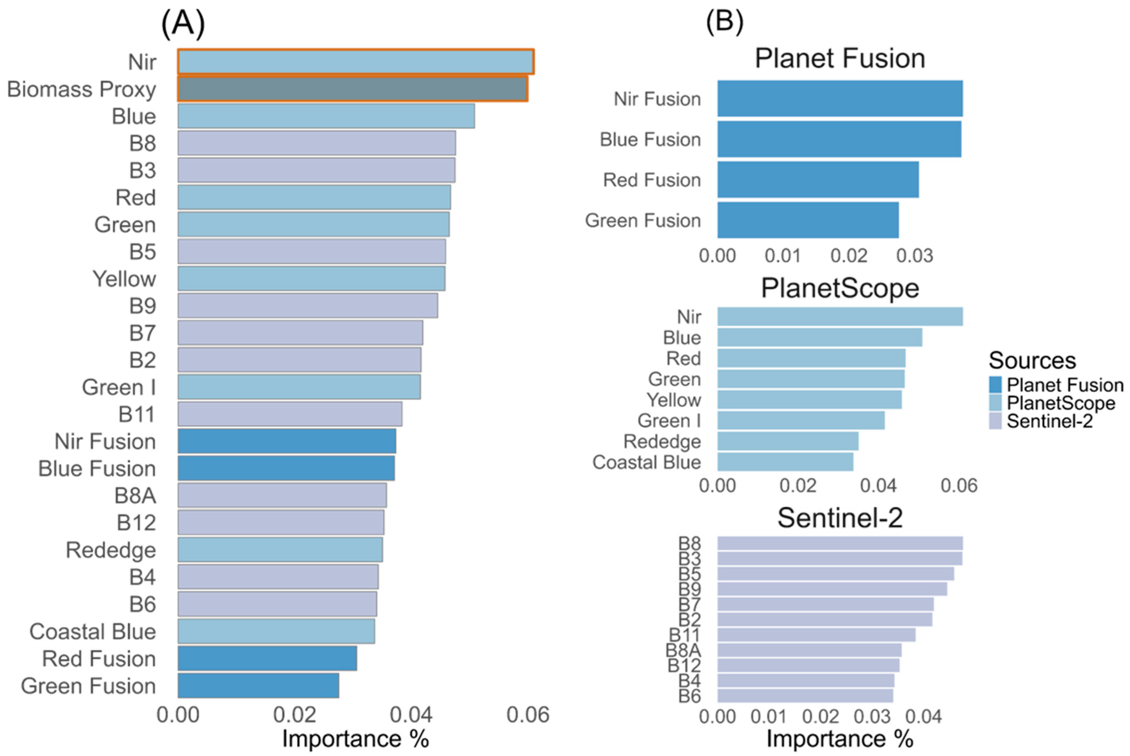
2.2.2. Feature Engineering

The datasets from each source were processed independently employing R statistics software [36]. In the case of Sentinel-2, the dataset was obtained from Google Earth Engine [37], and Biomass Proxy, PlanetScope, and Planet Fusion were obtained through Planet’s platform. The first steps were determining the interested area, georeferenced sampling points, and sampling dates. As mentioned, each satellite data source has a different number of spectral bands. Therefore, the “investigate_var_importance” function from the bartMachine R package [29] was employed to perform a feature selection and recognize the most relevant spectral bands for estimating biomass in alfalfa.

Furthermore, a permutation importance cross-validation through “var_selection_by_permute_cv” from the bartMachine R package [38] was applied to improve the robustness of feature selection. This permutation allows minimizing autocorrelation and spatial dimensionality within variables to obtain fewer inputs to build a model in a simpler way [39].

To calibrate the BART models, the hyperparameter tuning process was performed to select the best coefficients. In addition, a grid search was created to establish different combinations between four hyperparameters (k, q, Nu, and Num of trees), obtaining each combination for each value in the range of hyperparameters. A detailed description of the hyperparameters fitted, implemented, and optimal values found can be seen in

Table 4. Hyperparameters, values, and optimized value incorporated within the BART model evaluation.

Hyperparameter	Values Implemented	Optimized Value
k	1–3–5–7–9	1
q	0.1–0.3–0.5–0.7–0.9	0.1
Nu	1–3–5–7–9	1
Num tress	1 to 100 (By steps of 3)	61

. For k and Nu, values from 1 to 10 were implemented, q comprised values between 0.1 and 0.9, and 1 to 100 was the interval to several trees. The resulting combinations were ranked by root mean squared error (RMSE), considering as the best combination the group of hyperparameters with the lowest RMSE.

2.2.3. Predictive Modeling

To improve the fit of the model while minimizing the risk of overfitting, nested cross-validation was implemented. This method consists of two levels of validation: an outer and an inner loop. The first step was to partition the dataset into k-field folds, which formed the outer loop. In this partitioning, each field and its corresponding samples (observations within a field) were treated as a separate test dataset, while the samples of the remaining fields were used for model training. The data were then partitioned again, this time into inner resample training and test datasets within each outer fold (Figure 3). The goal of the inner loop was to optimize the hyperparameters of the model by testing each combination three times, using two fields for training and one field for testing [40]. The final selection was made based on the combination of hyperparameters that minimized the median root mean square error (RMSE). This approach allowed the construction of three optimized models, one for each array.

A regression model for biomass yield forecasting was constructed using the ‘bartMachine’ function from the bartMachine R package [38], incorporating the optimal parameters determined in the preview stages. The two main predictor variables employed were Planet’s PlanetScope Near-Infrared band and Biomass Proxy product. The primary output of this model, indicative of dry biomass yield, was derived from the length of the 95% credible intervals within the respective distributions, thus providing a probability level for each outcome. The mathematical expression of the BART model can be encapsulated in the following Equation [26].

$$Y=f\left(x\right)+\epsilon =SUM\left(G\left(x;Tj,Mj\right)\right)+\epsilon with \epsilon ~N\left(0,\sigma 2\right)$$

(1)

where $Tj$ is the _jth binary tree structure containing a set of terminal nodes and splitting rules, and $Mj$ = {U_j1, …, U_jbj} denotes a set of parameters of the b_j terminal nodes associated with $Tj$. To regularize the fit of each single tree using prior distributions, BART aims, so that each tree only explains a small part of the variation in the dependent variable.

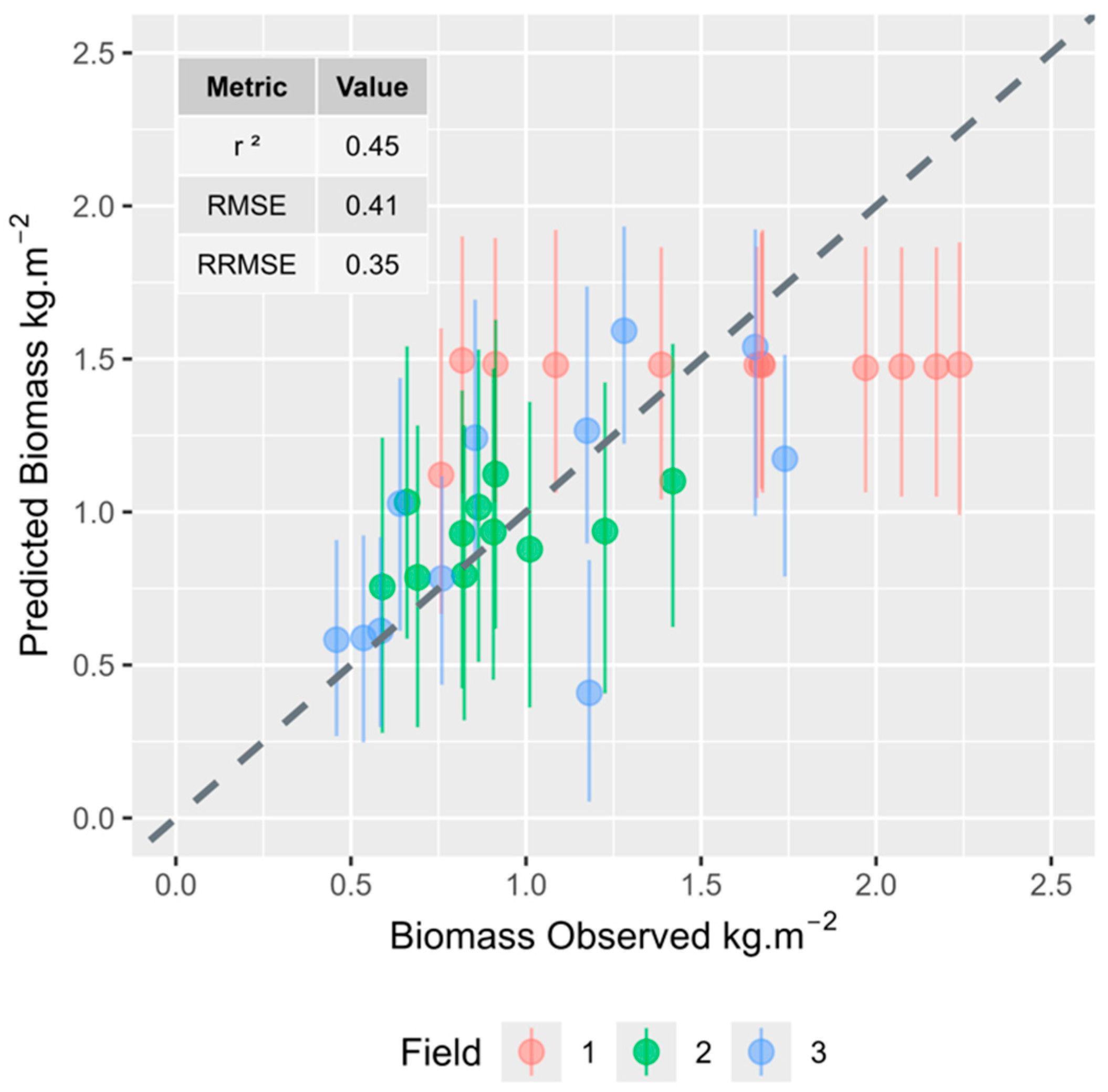
2.2.4. Performance Metrics

Six model performance metrics were employed: the Pearson correlation coefficient (r², Equation (2)), the Root Mean Square Error (RMSE, Equation (3)), the Relative RMSE (RRMSE, Equation (4)), the Pseudo r² (Equation (5)), pi lower, and pi upper.

$$r^2={\displaystyle \frac{SSR}{SST}}={\displaystyle \frac{\sum {\left({\widehat{y}}_i-y\right)}^2}{\sum {\left(y_i-\widehat{y}\right)}^2}}$$

(2)

where SSR (residual) is the sum of squared residuals, representing the amount of variability unexplained by the model, and SST (total), is the total sum of squares, which is the total amount of variability in the dependent variable.

$$RMSE=\sqrt{{\displaystyle \frac{{\sum }_{i=1}^n {\left({\widehat{y}}_i-y_i\right)}^2}{n}}}$$

(3)

where ${\widehat{y}}_i$ is the predicted response, $y_{i }$ is the observed response, and n is the number of samples.

$$RRMSE=\sqrt{{\displaystyle \frac{\frac{1}{n}{\sum }_{i=1}^n {\left(y_i-{\widehat{y}}_i\right)}^2}{{\sum }_{1=1}^n {\left({\widehat{y}}_i\right)}^2}}}$$

(4)

where ${\widehat{y}}_i$ is the predicted response, $y_i$ is the observed response, and n is the number of samples.

$${Pseudo r}^2={\displaystyle \frac{1-SEE}{SST}}$$

(5)

where $SEE$ is the sum of squared errors in the training data and $SST$ is the total sum of squares or the sample variance of the response multiplied by n − 1.

PI: The credible interval, derived from the BART posterior probability and defined between the lower and upper values. Represents the range where there is a 95% probability of containing the true population parameter.

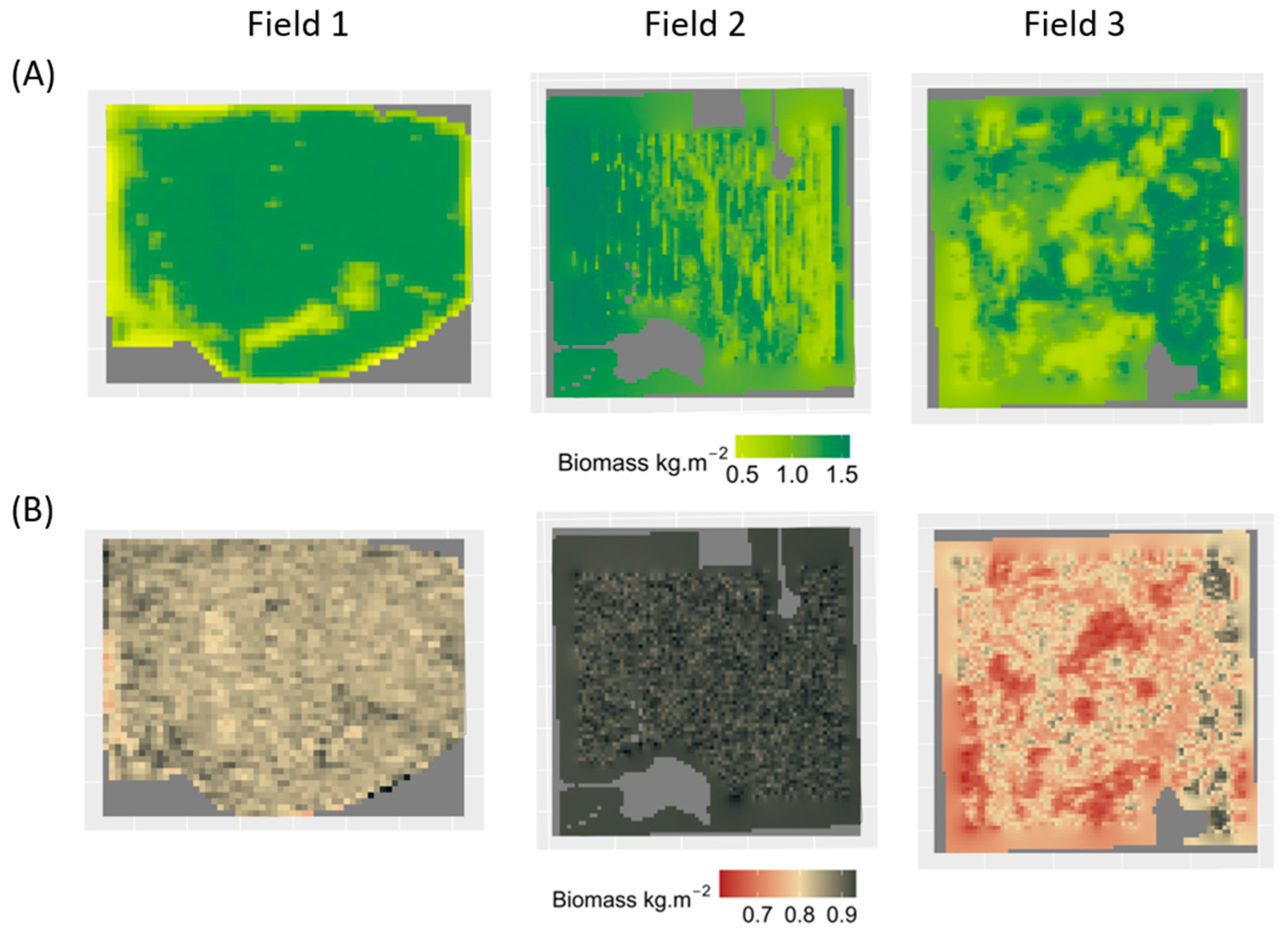
2.2.5. Framework Case Study

Finally, the first biomass sampling was selected to showcase the model’s functionality. Firstly, the biomass values from the first sampling date were compared to their predicted counterparts, and the performance metrics listed in Section 2.2.4 were evaluated. Secondly, the corresponding predictive and uncertainty maps of alfalfa biomass for each field were built. The size of the map pixels was 10 m⁻², composing fields of 3500, 4000, and 3700 pixels. The uncertainty maps were built considering the difference between minimum and maximum uncertainty values from the model.

3. Results

3.1. Biomass Statistics

The values of alfalfa biomass exhibited large variations in yield across the different measurements, ranging from 0.03 (dryland field 3;

Table 5. Dates, means, standard deviation, minimum, and maximum values of biomass obtained through samplings in the different fields. The values are expressed in kg m⁻².

Field	Date	Mean	Standard Deviation	Minimum	Maximum
1	3 May 2022	1.62	0.6	0.76	2.65
	13 June 2022	1.46	0.19	1.06	1.75
	8 July 2022	0.97	0.26	0.26	1.2
	27 July 2022	1	0.2	0.73	1.28
	30 August 2022	0.7	0.26	0.25	1.24
2	13 May 2022	0.9	0.24	0.59	1.42
	14 June 2022	0.92	0.36	0.41	1.41
3	16 May 2022	0.99	0.45	0.46	1.74
	14 June 2022	0.85	0.28	0.37	1.39
	27 July 2022	0.25	0.19	0.03	0.59
Overall		0.98	0.3	0.03	2.64

) to 2.65 kg m⁻² (irrigated field 1; Table 5), with a mean of 0.98 kg m⁻² and a standard deviation of 0.3 kg m⁻². The highest standard deviation in a sampling corresponded to the first sampling of Field 1 (0.6 kg m⁻²), whereas the overall standard deviation was 0.30 kg m⁻². Table 5 presents a summary of the sampling results.

3.2. Feature Selection

The variable importance through the feature selection showed large differences among remote sensing bands and products. The feature importance retrieved from the trained model between alfalfa biomass and spectral bands and different data sources is shown in Figure 4A. The bands with the higher importance corresponded to PlanetScope and Biomass Proxy. NIR from PlanetScope and Biomass proxy presented 6% importance each (Figure 4). Figure 4B shows the bands’ importance comparison expressed in percentage across evaluated sources. Contrastingly, Planet Fusion’s contribution was lower in comparison with the other sources, and it did not present a band with outstanding performance (<4%).

3.3. Model Development

The trained model shows promising results for effectively estimating biomass yield. Figure 5 shows a relation between observed and fitted values, with a trend in the model to underpredict biomass over 1.6 kg m⁻². The model performance results were: r²: 0.61, RMSE: 0.29 kg m⁻², and pseudo r² inner: 0.85. (Figure 5).

3.4. Case Study

Values extracted from the first sampling date were compared with predictions of the model. Figure 6 represents the benchmarking between those points. The performance results were: r²: 0.45, RMSE: 0.41 kg m⁻², and RRMSE: 0.35. Similar to Figure 5, there was a trend to underpredict biomass over 1.6 kg m⁻². Lastly, Figure 7A shows predicted biomass maps, identifying areas of lower (0.5 kg m⁻²; Field 3 Figure 7A) and higher productivity (1.6 kg m⁻²; Field 1 Figure 7A). The total biomass obtained was 3810 kg ha⁻², 3230 kg ha⁻², and 4340 kg ha⁻² for fields 1, 2, and 3, respectively. Figure 7B presents biomass uncertainty maps, with variations in the predicted biomass from 0.6 kg m⁻² to 1.1 kg m⁻². Field 2 had the highest uncertainties (1.08 kg m⁻²; Figure 7B) while Field 3 showed the lowest (0.61 kg m⁻²; Figure 7B). Notably, Field 1 has reduced variability in biomass prediction and is linked to stable uncertainty. Field 2 showed low biomass estimates with high uncertainty. Conversely, Figure 3 demonstrates greater variability in biomass prediction, suggesting more accurate estimations associated with low to medium uncertainty.

4. Discussion

This study presents a novel framework to estimate biomass yield, incorporating ground truth data collection, a robust cross-validation scheme, and a hyperparameter tuning approach to obtain a predictive model from a small dataset. The framework includes an ensemble nested method [41] that addresses model overfitting and spatial autocorrelation among variables [8,42]. This study proposes a validation approach that helps in selecting the best model by identifying the optimal combination of hyperparameters, mainly under reduced-size datasets. This method effectively utilizes the whole dataset for training and testing, yet in different stages, resulting in better hyperparameter tuning [43]. Moreover, overfitting problems can lead to performance deficiencies, making robust non-parametric methods crucial for validating, selecting, and evaluating predictive accuracy [44]. In this regard, BART provides much richer information than classical regression methods [45], as they incorporate uncertainty quantification [46], providing credible intervals to improve estimation accuracy by supplying a flexible database [47]. The findings of this study offer a promising solution to the challenges encountered in remote sensing and pasture modeling publications due to small experimental datasets, paving the way for future research avenues.

When working with remote sensing, it is essential to consider the vast array of satellite products and resources available today. This study provided insights regarding the performance of spectral bands for estimating alfalfa biomass, while previous efforts focused on ranking vegetation indexes [48]. Despite the work that has been carried out, a better understanding of the spectral reflectance saturation of vegetation remains a challenge. Variability in spectral reflectance saturation depends on a sensor type and vegetation structure [49]. The superior results of PlanetScope NIR and Biomass-Proxy are not only due to the higher geometric resolution that better matches the sample areas, but also due to the ability to adjust the pixel purity, which measures the degree of homogeneity with respect to the target crop. The results show that the optimal pixel size and wavelengths are not universal and vary from crop to crop. Therefore, it is reasonable to conclude that the PlanetScope NIR and Biomass-Proxy stand out for their geometric and spectral resolution as they relate to specific crops [50,51]. The assessment of biomass in crops such as alfalfa requires the consideration of different wavelengths, as observed by Tedeco et al. (2022) [52]. In concordance with this study results, a more comprehensive analysis by She et al. (2020) [53] ranked the B8 (Sentinel-2) band as crucial in determining yield estimation and crop management for crops such as corn, soybean, and rice. Additionally, Sentinel-2 proved superior to SAR (Sentinel-1) in explaining crop changes due to the latter’s complexities in image processing and interpretation [54]. A recent review by Tedesco et al. (2022) [54] found that Sentinel-2 bands were especially relevant for predicting alfalfa biomass. In this study, we found that PlanetScope NIR band and the radar-based Biomass Proxy product were the most important features in predicting alfalfa biomass. The relevant bands in this study were selected using permutation importance for selecting stable features [55]. This approach enables the comparison and selection of the most important bands from widely used data sources to estimate alfalfa biomass yield-reducing multicollinearity issues.

Predicting alfalfa biomass based on remote sensing products has been a challenging task with varying levels of performance reported in the literature (R² from 0.39 to 0.85; RMSE from 143 kg ha⁻² to 330 kg ha⁻²) [5,56,57,58]. Sileshi et al. (2014) [59] identified several common errors in the development of biomass regression models. These errors include an arbitrary selection of analytical methods, inadequate model evaluation, failure to account for collinearity, uncritical application of model selection criteria, and insufficient presentation of results. In our study, we tried to avoid these confusions. Therefore, our potential errors are likely more closely tied to the limited size of the dataset. Among these previous studies, a major weakness is the lack of spatial measurements of uncertainty in their predictions. The present study amends this limitation by employing a BART approach. Recent research has demonstrated that BART approaches can successfully predict coverage using remote sensing imagery and field data [60]. Remote sensing imagery and the Bayesian approach have also been applied to crops such as maize and sorghum to obtain regressions and uncertainty intervals in predictions [61,62]. This methodology has outperformed other methods, such as gradient-boosting machines and random forests, as evaluated on different datasets [63]. Not only does this instill confidence in its robustness and reliability, but it can also provide valuable insights into the spatial uncertainty associated with the predictions.

A few limitations of this study were related to the limited availability of ground truth data, exploring different environments, and cutting times during the growing season. The spatial transference of this model to other fields is limited to the training dataset, and further testing is needed in order to use this model with values of biomass beyond the range explored in this study. Therefore, future efforts should be made to explore more extensive geographic coverage and sampling moments during the growing season. The integration of new data leads to continual improvement in predictions over time, thus offering more accurate insights for management [39]. Furthermore, incorporating data from weather (such as precipitation, accumulated radiation, and temperatures), crop management information (e.g., days after sowing), soil variables, and weather could improve the prediction performance [16,64]. All these efforts contribute to developing a nondestructive tool for determining alfalfa cutting time using satellite imagery.

5. Conclusions

This study described an innovative framework to develop predictive models from small datasets. Through implementing nested cross-validation with a hyperparameter tuning optimization in the same approach, this study obtained promising estimation results (r²: 0.61; RMSE: 0.29 kg m⁻²), despite its small ground truth dataset. In addition, the proposed framework provides the uncertainty quantification to assess the range of error in the predictions. Furthermore, another outcome of this study is the comparison of different bands and satellite products. In this regard, PlanetScope NIR band and Biomass Proxy from Planet were used to train the model. Future steps should focus on expanding the spatial footprint of the observed data and include sampling moments in different crop stages. Finally, the proposed method represents a first step towards developing a nondestructive tool for determining alfalfa cutting time using satellite imagery.

References

1. Elfanssi, S.; Ouazzani, N.; Mandi, L. Soil properties and agro-physiological responses of alfalfa (Medicago sativa L.) irrigated by treated domestic wastewater. Agric. Water Manag. 2018, 202, 231–240. [Google Scholar] [CrossRef]
2. Zhang, J.; Wang, Q.; Pang, X.P.; Xu, H.P.; Wang, J.; Zhang, W.N.; Guo, Z.G. Effect of partial root-zone drying irrigation (PRDI) on the biomass, water productivity and carbon, nitrogen and phosphorus allocations in different organs of alfalfa. Agric. Water Manag. 2021, 243, 106525. [Google Scholar] [CrossRef]
3. Arshad, M.; Feyissa, B.A.; Amyot, L.; Aung, B.; Hannoufa, A. MicroRNA156 improves drought stress tolerance in alfalfa (Medicago sativa) by silencing SPL13. Plant Sci. 2017, 258, 122–136. [Google Scholar] [CrossRef] [PubMed]
4. Avci, M.A.; Ozkose, A.; Tamkoc, A. Determination of yield and quality characteristics of alfalfa (Medicago sativa L.) varieties grown in different locations. J. Anim. Vet. Adv. 2013, 12, 487–490. [Google Scholar]
5. Noland, R.L.; Wells, M.S.; Coulter, J.A.; Tiede, T.; Baker, J.M.; Martinson, K.L.; Sheaffer, C.C. Estimating alfalfa yield and nutritive value using remote sensing and air temperature. Field Crops Res. 2018, 222, 189–196. [Google Scholar] [CrossRef]
6. Oates, L.G.; Undersander, D.J.; Gratton, C.; Bell, M.M.; Jackson, R.D. Management-intensive rotational grazing enhances forage production and quality of subhumid cool-season pastures. Crop Sci. 2011, 51, 892–901. [Google Scholar] [CrossRef]
7. Caddel, J.; Stritzke, J.; Berberet, R.; Bolin, P.; Huhnke, R.; Johnson, G.; Cuperus, G. Alfalfa Production Guide for the Southern Great Plains. 2001, 71, E-826. Available online: https://extension.okstate.edu/fact-sheets/print-publications/e/e-826-2018.pdf (accessed on 28 August 2024).
8. Gou, J.; Debnath, S.; Sun, L.; Flanagan, A.; Tang, Y.; Jiang, Q.; Wen, J.; Wang, Z. From model to crop: Functional characterization of SPL 8 in M. truncatula led to genetic improvement of biomass yield and abiotic stress tolerance in alfalfa. Plant Biotechnol. J. 2018, 16, 951–962. [Google Scholar] [CrossRef]
9. Lorenzo, C.D.; García-Gagliardi, P.; Antonietti, M.S.; Sánchez-Lamas, M.; Mancini, E.; Dezar, C.A.; Vazquez, M.; Watson, G.; Yanovsky, M.J.; Cerdán, P.D. Improvement of alfalfa forage quality and management through the down-regulation of Ms FT a1. Plant Biotechnol. J. 2020, 18, 944–954. [Google Scholar] [CrossRef]
10. Diatta, A.A.; Min, D.; Jagadish, S.V.K. Drought stress responses in non-transgenic and transgenic alfalfa—Current status and future research directions. In Advances in Agronomy; Elsevier: Amsterdam, The Netherlands, 2021; Volume 170, pp. 35–100. [Google Scholar] [CrossRef]
11. Katanski, S.; Milić, D.; Vasiljević, S.; Milošević, B.; Živanov, D.; Ćupina, B. Dry matter yield and plant density of alfalfa as affected by cutting schedule and seeding rate. In Proceedings of the 27th General Meeting of the European Grassland Federation “Sustainable Meat and Milk Production from Grasslands”, Cork, Ireland, 17–21 June 2018; Teagasc, Animal and Grassland Research and Innovation Centre: Cork, Ireland, 2018; Volume 23, pp. 265–267. [Google Scholar]
12. Ramoelo, A.; Cho, M.A.; Mathieu, R.; Madonsela, S.; Van De Kerchove, R.; Kaszta, Z.; Wolff, E. Monitoring grass nutrients and biomass as indicators of rangeland quality and quantity using random forest modelling and WorldView-2 data. Int. J. Appl. Earth Obs. Geoinf. 2015, 43, 43–54. [Google Scholar] [CrossRef]
13. Reinermann, S.; Asam, S.; Kuenzer, C. Remote Sensing of Grassland Production and Management—A Review. Remote Sens. 2020, 12, 1949. [Google Scholar] [CrossRef]
14. Song, X.P.; Huang, W.; Hansen, M.C.; Potapov, P. An evaluation of Landsat, Sentinel-2, Sentinel-1 and MODIS data for crop type mapping. Sci. Remote Sens. 2021, 3, 100018. [Google Scholar] [CrossRef]
15. Wang, X.; Lei, H.; Li, J.; Huo, Z.; Zhang, Y.; Qu, Y. Estimating evapotranspiration and yield of wheat and maize croplands through a remote sensing-based model. Agric. Water Manag. 2023, 282, 108294. [Google Scholar] [CrossRef]
16. Whitmire, C.D.; Vance, J.M.; Rasheed, H.K.; Missaoui, A.; Rasheed, K.M.; Maier, F.W. Using Machine Learning and Feature Selection for Alfalfa Yield Prediction. AI 2021, 2, 71–88. [Google Scholar] [CrossRef]
17. Sivasankar, T.; Lone, J.M.; Sarma, K.K.; Qadir, A.; Raju, P.L.N. Estimation of Above Ground Biomass Using Support Vector Machines and ALOS/PALSAR data. Vietnam J. Earth Sci. 2019, 41, 95–104. [Google Scholar] [CrossRef]
18. Hernandez, C.M.; Correndo, A.; Kyveryga, P.; Prestholt, A.; Ciampitti, I.A. On-farm soybean seed protein and oil prediction using satellite data. Comput. Electron. Agric. 2023, 212, 108096. [Google Scholar] [CrossRef]
19. Xu, J.; Quackenbush, L.J.; Volk, T.A.; Im, J. Forest and Crop Leaf Area Index Estimation Using Remote Sensing: Research Trends and Future Directions. Remote Sens. 2020, 12, 2934. [Google Scholar] [CrossRef]
20. Gao, F.; Zhang, X. Mapping Crop Phenology in Near Real-Time Using Satellite Remote Sensing: Challenges and Opportunities. J. Remote Sens. 2021, 2021, 8379391. [Google Scholar] [CrossRef]
21. Lu, D. The potential and challenge of remote sensing-based biomass estimation. Int. J. Remote Sens. 2006, 27, 1297–1328. [Google Scholar] [CrossRef]
22. Wu, W.; Tang, X.; Lv, J.; Yang, C.; Liu, H. Potential of Bayesian additive regression trees for predicting daily global and diffuse solar radiation in arid and humid areas. Renew. Energy 2021, 177, 148–163. [Google Scholar] [CrossRef]
23. Jia, X.; Zhang, Z.; Wang, Y. Forage yield, canopy characteristics, and radiation interception of ten alfalfa varieties in an arid environment. Plants 2022, 11, 1112. [Google Scholar] [CrossRef]
24. Andersen, R. Nonparametric methods for modeling nonlinearity in regression analysis. Annu. Rev. Sociol. 2009, 35, 67–85. [Google Scholar] [CrossRef]
25. Mancino, G.; Falciano, A.; Console, R.; Trivigno, M.L. Comparison between parametric and non-parametric supervised land cover classifications of sentinel-2 msi and landsat-8 oli data. Geographies 2023, 3, 82–109. [Google Scholar] [CrossRef]
26. Chipman, H.A.; George, E.I.; McCulloch, R.E. BART: Bayesian additive regression trees. Ann. Appl. Stat. 2010, 4, 266–298. [Google Scholar] [CrossRef]
27. Makowski, D.; Jeuffroy, M.-H.; Guérif, M. Bayesian methods for updating crop-model predictions, applications for predicting biomass and grain protein content. Frontis 2004, 3, 57–68. [Google Scholar]
28. Correndo, A.A.; Tremblay, N.; Coulter, J.A.; Ruiz-Diaz, D.; Franzen, D.; Nafziger, E.; Prasad, V.; Rosso, L.H.M.; Steinke, K.; Du, J.; et al. Unraveling uncertainty drivers of the maize yield response to nitrogen: A Bayesian and machine learning approach. Agric. For. Meteorol. 2021, 311, 108668. [Google Scholar] [CrossRef]
29. Hamilton, V.L.; Kansas Agricultural Experiment Station; United States. Soil Survey, Wichita County, Kansas. U.S. Dept. of Agriculture, Soil Conservation Service. 1965. Available online: https://catalog.hathitrust.org/Record/101740228 (accessed on 10 February 2024.).
30. Kansas Mesonet. Available online: https://mesonet.k-state.edu/ (accessed on 20 December 2022).
31. Córdoba, M.; Vega, A.; Balzarini, M. Protocolo de Análisis para la Delimitación de Zonas de Manejo Intralote; Conference: XIX Reunión Científica del GABAt: Santiago del Estero, Argentina, 2014. [Google Scholar] [CrossRef]
32. Planet Fusion Monitoring Technical Specifications. 2021. Available online: https://assets.planet.com/docs/Planet_fusion_specification_March_2021.pdf (accessed on 15 December 2022).
33. Roy, D.P.; Huang, H.; Houborg, R.; Martins, V.S. A global analysis of the temporal availability of PlanetScope high spatial resolution multi-spectral imagery. Remote Sens. Environ. 2021, 264, 112586. [Google Scholar] [CrossRef]
34. Burger, R.; Aouizerats, B.; Den Besten, N.; Guillevic, P.; Catarino, F.; Van Der Horst, T.; Jackson, D.; Koopmans, R.; Ridderikhoff, M.; Robson, G.; et al. The Biomass Proxy: Unlocking Global Agricultural Monitoring through Fusion of Sentinel-1 and Sentinel-2. Remote Sens. 2024, 16, 835. [Google Scholar] [CrossRef]
35. Gatti, A.; Bertolini, A. Sentinel-2 Products Specification Document; Thales Alenia Space: Cannes, France, 2018; pp. 1–487. [Google Scholar]
36. R Core Team. R: A Language and Environment for Statistical Computing; R Foundation for Statistical Computing: Vienna, Austria, 2021; Available online: https://www.R-project.org/ (accessed on 12 September 2022).
37. Aybar, C.; Wu, Q.; Bautista, L.; Yali, R.; Barja, A. rgee: An R package for interacting with Google Earth Engine. J. Open Source Softw. 2020, 5, 2272. [Google Scholar] [CrossRef]
38. Kapelner, A.; Bleich, J. bartMachine: Machine Learning with Bayesian Additive Regression Trees. J. Stat. Softw. 2016, 70, 1–40. [Google Scholar] [CrossRef]
39. Debeer, D.; Strobl, C. Conditional permutation importance revisited. BMC Bioinform. 2020, 21, 307. [Google Scholar] [CrossRef]
40. Zhong, Y.; He, J.; Chalise, P. Nested and Repeated Cross Validation for Classification Model with High-Dimensional Data. Rev. Colomb. Estad. 2020, 43, 103–125. [Google Scholar] [CrossRef]
41. Dinh, T.L.A.; Aires, F. Nested leave-two-out cross-validation for the optimal crop yield model selection. Geosci. Model Dev. 2022, 15, 3519–3535. [Google Scholar] [CrossRef]
42. Roberts, J.; Curran, M.; Poynter, S.; Moy, A.; Ommen, T.V.; Vance, T.; Tozer, C.; Graham, F.S.; Young, D.A.; Plummer, C.; et al. Correlation confidence limits for unevenly sampled data. Comput. Geosci. 2017, 104, 120–124. [Google Scholar] [CrossRef]
43. Trachsel, M.; Telford, R.J. Technical note: Estimating unbiased transfer-function performances in spatially structured environments. Clim. Past 2016, 12, 1215–1223. [Google Scholar] [CrossRef]
44. Hastie, T.; Tibshirani, R.; Friedman, J. The Elements of Statistical Learning; Springer: New York, NY, USA, 2009. [Google Scholar] [CrossRef]
45. Mazzara, M.; Bruel, J.-M.; Meyer, B.; Petrenko, A. Software Technology: Methods and Tools. In Proceedings of the 51st International Conference, TOOLS 2019, Innopolis, Russia, 15–17 October 2019; Volume 11771. [Google Scholar] [CrossRef]
46. Williams, B.K.A.; Eaton, M.J.; Breininger, D.R. Adaptive resource management and the value of information. Ecol. Model. 2011, 222, 3429–3436. [Google Scholar] [CrossRef]
47. Shirley, R.; Pope, E.; Bartlett, M.; Oliver, S.; Quadrianto, N.; Hurley, P.; Duivenvoorden, S.; Rooney, P.; Barrett, A.B.; Kent, C.; et al. An empirical, Bayesian approach to modelling crop yield: Maize in USA. Environ. Res. Commun. 2020, 2, 025002. [Google Scholar] [CrossRef]
48. Feng, L.; Zhang, Z.; Ma, Y.; Du, Q.; Williams, P.; Drewry, J.; Luck, B. Alfalfa Yield Prediction Using UAV-Based Hyperspectral Imagery and Ensemble Learning. Remote Sens. 2020, 12, 2028. [Google Scholar] [CrossRef]
49. Mutanga, O.; Masenyama, A.; Sibanda, M. Spectral saturation in the remote sensing of high-density vegetation traits: A systematic review of progress, challenges, and prospects. ISPRS J. Photogramm. Remote Sens. 2023, 198, 297–309. [Google Scholar] [CrossRef]
50. Duveiller, G.; Defourny, P. A conceptual framework to define the spatial resolution requirements for agricultural monitoring using remote sensing. Remote Sens. Environ. 2010, 114, 2637–2650. [Google Scholar] [CrossRef]
51. Löw, F.; Duveiller, G. Defining the spatial resolution requirements for crop identification using optical remote sensing. Remote Sens. 2014, 6, 9034–9063. [Google Scholar] [CrossRef]
52. Tedesco, D.; Nieto, L.; Hernández, C.; Rybecky, J.F.; Min, D.; Sharda, A.; Ciampitti, I.A. Remote sensing on alfalfa as an approach to optimize production outcomes: A review of evidence and directions for future assessments. Remote Sens. 2022, 14, 4940. [Google Scholar] [CrossRef]
53. She, B.; Yang, Y.; Zhao, Z.; Huang, L.; Liang, D.; Zhang, D. Identification and mapping of soybean and maize crops based on Sentinel-2 data. Int. J. Agric. Biol. Eng. 2020, 13, 171–182. [Google Scholar] [CrossRef]
54. Steele-Dunne, S.C.; McNairn, H.; Monsivais-Huertero, A.; Judge, J.; Liu, P.-W.; Papathanassiou, K. Radar Remote Sensing of Agricultural Canopies: A Review. IEEE J. Sel. Top. Appl. Earth Obs. Remote Sens. 2017, 10, 2249–2273. [Google Scholar] [CrossRef]
55. Zhong, Y.; Chalise, P.; He, J. Nested cross-validation with ensemble feature selection and classification model for high-dimensional biological data. Commun. Stat.—Simul. Comput. 2023, 52, 110–125. [Google Scholar] [CrossRef]
56. Azadbakht, M.; Ashourloo, D.; Aghighi, H.; Homayouni, S.; Shahrabi, H.S.; Matkan, A.; Radiom, S. Alfalfa yield estimation based on time series of Landsat 8 and PROBA-V images: An investigation of machine learning techniques and spectral-temporal features. Remote Sens. Appl. Soc. Environ. 2022, 25, 100657. [Google Scholar] [CrossRef]
57. Li, J.; Wang, R.; Zhang, M.; Wang, X.; Yan, Y.; Sun, X.; Xu, D. A Method for Estimating Alfalfa (Medicago sativa L.) Forage Yield Based on Remote Sensing Data. Agronomy 2022, 13, 2597. [Google Scholar] [CrossRef]
58. Sapkota, A.; Haghverdi, A.; Montazar, A. Estimating fall-harvested alfalfa (Medicago sativa L.) yield using unmanned aerial vehicle–based multispectral and thermal images in southern California. Agrosystems Geosci. Environ. 2023, 6, e20392. [Google Scholar] [CrossRef]
59. Sileshi, G.W. A critical review of forest biomass estimation models, common mistakes and corrective measures. For. Ecol. Manag. 2014, 329, 237–254. [Google Scholar] [CrossRef]
60. McCord, S.E.; Buenemann, M.; Karl, J.W.; Browning, D.M.; Hadley, B.C. Integrating Remotely Sensed Imagery and Existing Multiscale Field Data to Derive Rangeland Indicators: Application of Bayesian Additive Regression Trees. Rangel. Ecol. Manag. 2017, 70, 644–655. [Google Scholar] [CrossRef]
61. Habyarimana, E.; Piccard, I.; Zinke-Wehlmann, C.; De Franceschi, P.; Catellani, M.; Dall’Agata, M. Early within-season yield prediction and disease detection using sentinel satellite imageries and machine learning technologies in biomass sorghum. In Software Technology: Methods and Tools: 51st International Conference, TOOLS, Innopolis, Russia, Proceedings 51; Springer International Publishing: Berlin/Heidelberg, Germany, 2019; pp. 227–234. [Google Scholar] [CrossRef]
62. Ma, Y.; Zhang, Z.; Kang, Y.; Özdoğan, M. Corn yield prediction and uncertainty analysis based on remotely sensed variables using a Bayesian neural network approach. Remote Sens. Environ. 2021, 259, 112408. [Google Scholar] [CrossRef]
63. Hill, J.; Linero, A.; Murray, J. Bayesian Additive Regression Trees: A Review and Look Forward. Annu. Rev. Stat. Its Appl. 2020, 7, 251–278. [Google Scholar] [CrossRef]
64. Vance, J.A.; Rasheed, K.; Missaoui, A.; Maier, F.W. Data Synthesis for Alfalfa Biomass Yield Estimation. AI 2022, 4, 1–15. [Google Scholar] [CrossRef]
Figure 1. (A) Geographical distribution of the fields in Kansas, United States, included in this study. (BD) show the spatial distribution of the samples within each field. The field in panel (B) was under irrigated conditions, while the fields in panels (C,D) were in dryland conditions.
Remotesensing 16 03379 g001
Figure 2. Conceptual framework of integrating and analyzing satellite and ground field data to obtain a biomass prediction model with the application at on-farm scale using a Bayesian approach.
Remotesensing 16 03379 g002
Figure 3. Nested cross-validation diagram. Example of split data holding one field and sample date out to create a training and testing set to tune hyperparameters.
Remotesensing 16 03379 g003
Figure 4. Importance between different spectral bands and alfalfa forage biomass. Panel (A) shows the band comparison across remote sensing sources. The orange highlighting of the first and second boxes identifies the two selected bands. Panel (B) shows the importance of the variables for each source independently. The colors stand for the source of the data (gray = Biomass Proxy, blue = Planet Fusion, light blue = PlanetScope, violet = Sentinel 2). Importance expressed in percentages.
Remotesensing 16 03379 g004
Figure 5. Accuracy evaluation of alfalfa regression model. Relation between observed and predicted biomass. The vertical lines represent the interval of 95 of the probability. Different colors (red = field 1, green = field 2, and blue = field 3) represent the data from the different fields. The dashed line is the 1:1 relation between observed and predicted values.
Remotesensing 16 03379 g005
Figure 6. Benchmarking was obtained between field biomass and model results for the first sampling date. The dashed line is a 1:1 relationship observed/ predicted. Color points represent different fields (red = field 1, green= field 2, and blue field 3). Units are expressed in kg m−2.
Remotesensing 16 03379 g006
Figure 7. (A) Predicted maps of alfalfa biomass. The colors range from yellow (low biomass) to green (high biomass). (B) Uncertainty maps of alfalfa biomass. The maps show the difference between the minimum and maximum prediction. Colors range from brown (low), and beige (intermediate) to black (high).
Remotesensing 16 03379 g007