Himawari-8 Sea Surface Temperature Products from the Australian Bureau of Meteorology

Abstract

As a contribution to the Integrated Marine Observing System (IMOS), the Bureau of Meteorology introduces new reprocessed Himawari-8 satellite-derived Sea Surface Temperature (SST) products. The Radiative Transfer Model and a Bayesian cloud clearing method is used to retrieve SSTs every 10 min from the geostationary satellite Himawari-8. An empirical Sensor Specific Error Statistics (SSES) model, introduced herein, is applied to calculate bias and standard deviation for the retrieved SSTs. The SST retrieval and compositing method, along with validation results, are discussed. The monthly statistics for comparisons of Himawari-8 Level 2 Product (L2P) skin SST against in situ SST quality monitoring (iQuam) in situ SST datasets, adjusted for thermal stratification, showed a mean bias of −0.2/−0.1 K and a standard deviation of 0.4–0.7 K for daytime/night-time after bias correction, where satellite zenith angles were less than 60° and the quality level was greater than 2. For ease of use, these native resolution SST data have been composited using a method introduced herein that retains retrieved measurements, to hourly, 4-hourly and daily SST products, and projected onto the rectangular IMOS 0.02 degree grid. On average, 4-hourly products cover ≈$10\%$ more of the IMOS domain, while one-night composites cover ≈$25\%$ more of the IMOS domain than a typical 1 h composite. All available Himawari-8 data have been reprocessed for the September 2015–December 2022 period. The 10 min temporal resolution of the newly developed Himawari-8 SST data enables a daily composite with enhanced spatial coverage, effectively filling in SST gaps caused by transient clouds occlusion. Anticipated benefits of the new Himawari-8 products include enhanced data quality for applications like IMOS OceanCurrent and investigations into marine thermal stress, marine heatwaves, and ocean upwelling in near-coastal regions.

1. Introduction

Sea Surface Temperature (SST) plays a vital role in numerical weather prediction, global climate modelling, and studies of climate change and variability. Satellite-derived SST measurements benefit a wide spectrum of operational and research applications, including ocean, weather, climate, and seasonal monitoring and forecasting, military operations, coral bleaching assessment, commercial fisheries and aquaculture, and environmental management. Geostationary satellites provide continuous observations of SST with finer temporal scales compared to polar orbiters, providing an invaluable opportunity for applications that require monitoring quickly evolving phenomena, such as ocean upwelling, marine heatwaves, and diurnal warming. This paper describes the new Himawari-8 geostationary satellite SST products from the Bureau of Meteorology (Bureau), which are generated using software based on the European Space Agency (ESA) Climate Change Initiative (CCI) SST version 2 processing code [1].

The Japanese geostationary satellites, Himawari-8 and Himawari-9 [2], offer significant improvements in frequency, resolution, and precision compared with their predecessors, the Multi-functional Transport Satellite (MTSAT) series. They are located at 140.7°E, and observe the Earth from ≈59.5°E to 222°E, and 81°N to 81°S. The optical radiometer, Advanced Himawari Imager (AHI), onboard Himawari-8/9, provides full disk images every 10 min with 2 km spatial resolution, as compared to the MTSAT series with a resolution of 4 km and temporal resolution of 20 min for infrared (IR) frequency data at nadir. It has 16 spectral bands for visible-infrared wavelengths, and of these, the IR bands centred at 3.9, 8.6, 10.4, 11.2, and 12.4 μm are able to sense SSTs. Himawari-8 started providing real-time data on 7 July 2015, while Himawari-9 was on standby. JMA officially replaced Himawari-8 with Himawari-9 on 12 December 2022. At present, several agencies are operationally generating various Himawari-8/9 SST datasets. These include the Japan Aerospace Exploration Agency (JAXA) [3], the National Oceanic and Atmospheric Administration (NOAA) [4], and the Bureau of Meteorology (Bureau), each using different retrieval algorithms. In response to user requests for a high-quality, consistent SST product over the Australian domain, we aim to produce such products from both current and future polar and geostationary platforms at the Bureau. Our goal here is to enhance our capability of producing consistent, high quality SST products from the geostationary platform Himawari-8.

The Bureau produces numerous high-resolution satellite-derived SST data products as a contribution to the Integrated Marine Observing System (IMOS). The Bureau originally produced Himawari-8 SST products in near real time from 2016, but they were not sufficiently accurate for assimilation into operational ocean models or SST analyses. For those legacy products (file version 3, “fv03”), SST was retrieved by regressing against one day of SST data from VIIRS in 2015. The Geostationary Cloud Algorithm Test-bed (GEOCAT) cloud mask [5] was used to detect clouds. This cloud product showed major systematic biases such as a tendency to misclassify boundary layer clouds, cirrus and multilayer cloud types and was not as accurate as other cloud products (e.g., [6]). There was no bias model applied to fv03 legacy product, so uncertainty in the observations was not available for users to decide the quality of data, as required by the International Group for High Resolution SST (GHRSST) [7].

We therefore looked at using the ESA SST CCI processing code which was developed at the University of Reading (UoR) to process Advanced Very High Resolution Radiometer (AVHRR) and Along-Track Scanning Radiometer (ATSR) data to form very accurate satellite-based time series of SST for the 1981–2016 period [1]. The Bureau is collaborating with the University of Reading to modify their SST retrieval methods to improve SST retrievals from Himawari-8 and Himawari-9 geostationary satellites. This paper describes the Bureau’s Level 2 and Level 3 file version 2 (“fv02”) SST products derived using IR data from the AHI sensor on Himawari-8, using an adaptation of the ESA CCI SST processing code version 2.

An empirical bias model based on in situ data were developed in the Bureau to define uncertainty values for every pixel that has valid values for SST, based on the bias model developed for IMOS AVHRR SSTs [8,9]. Using the new merging method developed at the Bureau [8,9], Level 3 composite SST products were further developed. Altogether, Level 2 Pre-processed (L2P) for each scene and Level 3 Collated (L3C) products for 1 h, 4 h, and 1-day night SST products in the GHRSST format (GDS 2.0, [7]) are produced every day with Himawari data. Usually, there are 142 L2P files, 24 L3C 01 h files, six L3C 04 h files and one night file per day.

The remainder of the paper is structured as follows: Section 2 describes methods used to retrieve SST from Himawari-8. A brief description of the RTTOV and Bayesian cloud clearing methods is given in this section. The data used for the SST retrieval process is described in Section 3. The SST retrieval process is outlined in Section 4. The Sensor Specific Error Statistics (SSES) bias model applied to the L2P Himawari-8 SST files is also described in Section 4, along with compositing methods. Resultant SST products and their validation with in situ data are discussed in Section 5. The discussion and conclusions are given in Section 6.

2. Methods

In collaboration with the University of Reading, the Bureau has developed a method to retrieve SSTs from Himawari-8 by using the fast radiative transfer model RTTOV v12.3 [10] for simulating top-of-atmosphere radiances from passive visible and infrared channels of the AHI radiometer on Himawari-8 and a Bayesian approach for detecting clouds to determine clear sky conditions. The optimal estimation and Bayesian cloud clearing method originally developed at the University of Reading for AVHRR and A(A)TSR sensors for SST CCI version 2.1 Climate Data Record [1] were modified so that they could be applied to the AHI sensor on Himawari-8.

The Himawari SST processor is adapted from the ESA SST CCI processor version 2 [1], which is a physically based method to infer skin Sea Surface Temperature (skin SST) at around 10 μm depth [11] from infrared imagery. The two main steps involved are cloud detection (to identify which parts of the image have sufficiently clear skies to estimate SST) and retrieval (the inversion of clear-sky brightness temperatures to infer information about the surface temperature and atmospheric state). Cloud detection is undertaken using a Bayesian calculation of the probability of the presence of cloud across the image [12,13]. SST retrieval is undertaken by optimal estimation [14], an inverse method that provides a value for SST with its uncertainty. Both algorithms are physically based, and use a fast radiative transfer model (RTTOV12.3) [10] to simulate the expected clear-sky radiances informed by numerical weather prediction fields. We used the Bureau’s Global Australian Community Climate and Earth-System Simulator versions APS1, APS2 and APS3 (ACCESS-G1, ACCESS-G2 and ACCESS-G3) meteorological variables (Section 3) as the prior information. The components of the processing chain required to implement these steps are now described in turn.

The Radiative Transfer for TIROS Operational Vertical Sounder (RTTOV) [10,15] has been used for applications such as data assimilation in numerical weather prediction (NWP) models [16] and enabling physical retrievals from satellite data [17]. RTTOV uses an atmospheric profile of temperature, humidity, cloud, and surface properties as state vectors, and simulates radiances for satellite visible, infrared, or microwave nadir scanning instruments. It is able to compute radiances for all channels and brightness temperatures (BTs) for thermal channels and reflectances for solar affected channels.

Detecting clouds is critical in the SST retrieval process as SST retrievals from infrared imagery are possible only for clear sky conditions. A physically based, probabilistic (Bayesian) approach [12] has been used for cloud detection to determine clear sky conditions [13,18]. In Bayesian approaches, satellite observations and prior knowledge of the atmospheric and surface conditions are used to estimate clear-sky probabilities. A single threshold is applied to these clear-sky probabilities to determine a binary cloud mask for SST retrieval. The incidence of both missed cloud and false detection of clouds are significantly less in the Bayesian approach than ‘threshold’-based traditional approaches (e.g., [19,20,21,22]) to cloud screening [18]. In part, this is because prior information employed in the Bayesian approach is dynamic rather than static, which helps with the generality of the method to a wide range of atmospheric conditions [12].

Optimal estimation (OE) is a robust and general inverse method widely applied in remote sensing [23] and data assimilation, and has been used for SST retrievals from IR satellite channels [14,24]. A forward model that includes a priori information about the ocean and atmospheric state is utilised to calculate simulated brightness temperature (BT). The sensitivity of the simulated BTs to the ocean and atmospheric state is also calculated. The difference between the observations and simulated BTs derived from the Radiative Transfer Model (RTM) applied to the full prior-state NWP profile and the sensitivity information are further combined to estimate the difference between the prior information about the state and the actual state, and thus to estimate the actual state. The OE method has significant advantages over the traditional regression based retrieval approach as it can estimate both retrieval uncertainty and sensitivity [25].

3. Data

Himawari-8 AHI Full Disk ‘Himawari Standard Data’ files, Level 1a data [2,26] are used as the source of Himawari-8 AHI data. The Global Australian Multi-Sensor Sea Surface Temperature Analysis (GAMSSA, [27,28]) foundation SST is a daily analysis SST product available on a global 0.25° grid. It is used as the level 4 SST analysis for the background SST field.

The Bureau’s Numerical Weather Prediction (NWP) model ACCESS-G1, ACCESS-G2 and ACCESS-G3 [29,30] data were used as input for the RTTOV model. ACCESS-G1 data were used for 1 September 2015 to 15 March 2016, ACCESS-G2 for 16 March 2016 to 22 July 2019, and ACCESS-G3 for 23 July 2019 to 12 December 2022. The hourly analysis and forecast meteorological variables—atmospheric temperature profile, atmospheric water vapour profile, log surface pressure, sea surface temperature, mean sea level pressure, sea ice cover, 10 m wind U-component, 10 m wind-V-component, 2 m air temperature, 2 m dew point temperature, skin temperature, specific humidity, and cloud specific liquid water content at height of hybrid theta levels (atmosphere_hybrid_height_coordinate) were provided as atmospheric and surface state data. ACCESS-G1 data are output in 12 h intervals at 40 km horizontal resolution, ACCESS-G2 data are output in 6 h intervals at 25 km horizontal resolution, while ACCESS-G3 data are output in 6 h intervals at 12 km spatial resolution, all for 70 model atmospheric levels [30,31,32].

Fractional sea ice cover (unitless) derived from near real-time UKMO Operational Sea Surface Temperature and Ice Analysis (OSTIA) Daily 0.05° L4 is used for ice masking. OSTIA fractional sea ice cover is an optimal interpolation of the operational near real-time EUMETSAT OSI-SAF SSMIS daily 10 km Level 3 sea ice concentration fields [33].

4. Principles for SST Estimates

4.1. SST Retrieval Process

The Bayesian cloud detection scheme is so named as it uses Bayes’ theorem to express the probability of clear-sky (c) given the observations ($\mathit{y}$) and available prior information (${\mathit{x}}_a$) as

$$P\left(c\right|\mathit{y},{\mathit{x}}_a)={\displaystyle \frac{P\left(\mathit{y}\right|{\mathit{x}}_a,c)P\left({\mathit{x}}_a\right|c)P\left(c\right)}{P\left(\mathit{y}\right|{\mathit{x}}_a)P\left({\mathit{x}}_a\right)}},$$

(1)

where the probability terms on the right-hand side may be estimated as detailed in [12]. The observation vector $\mathit{y}$ consists of the satellite observations, and the background state vector ${\mathit{x}}_a$ includes the prior sea surface temperature, total column water vapour (TCWV), and windspeed from Bureau’s NWP model data. The equation simplifies assuming $P\left({\mathit{x}}_a\right|c)=P\left({\mathit{x}}_a\right)$ as the NWP data with length scales ∼10 to ∼100 km cannot resolve cloud structures at the pixel scales ∼1 to ∼10 km. The denominator is the sum of the two possible classes (clear or “not clear”),

$$P\left(\mathit{y}\right|{\mathit{x}}_a)=P\left(\mathit{y}\right|{\mathit{x}}_a,c)P\left(c\right)+P\left(\mathit{y}\right|{\mathit{x}}_a,\overline{c})P\left(\overline{c}\right),$$

(2)

The observation vector $\mathit{y}$ includes both spectral and textural information. The brightness temperatures observed by the five thermal channels correspond to five elements of the observation vector for a specific pixel. Five of the Himawari channels are used for the spectral observations: 0.64, 0.86, 3.9, 10.4, and 12.4 μm. We denote this subset of the observation vector as ${\mathit{y}}_s$, where the s signifies spectral elements because they represent samples from the brightness temperature spectrum. We also incorporated texture (multipixel information) measures as elements in the observation vector. Cloudy regions tend to exhibit greater spatial variability compared to clear-sky regions, making texture measures informative. The local standard deviation in a 3 × 3 pixel box for the 10.4 μm channel provides the textural information ${\mathit{y}}_t$ in our case. ${\mathit{y}}_s$ and ${\mathit{y}}_t$ are assumed to be independent, such that $P\left(\mathit{y}\right|{\mathit{x}}_a,c)=P\left({\mathit{y}}_s\right|{\mathit{x}}_a,c)P\left({\mathit{y}}_t\right|{\mathit{x}}_a,c)$.

The clear-sky spectral probability density functions (PDFs) can be estimated from the RTM output. Simulating top-of-atmosphere radiances on-the-fly for cloudy conditions is computationally expensive. The textural and cloudy-sky PDFs are therefore evaluated from pre-generated lookup tables. The clear-sky spectral PDF is

$$P\left({\mathit{y}}_S\right|{\mathit{x}}_a,c)={\displaystyle \frac{\exp \left(-0.5{(\mathit{y}-F\left({\mathit{x}}_a\right))}^T{({\mathit{KS}}_a{\mathit{K}}^T+{\mathit{S}}_{ϵ})}^{-1}(\mathit{y}-F\left({\mathit{x}}_a\right))\right)}{{\left(2\pi \right)}^{\frac{n}{2}}{|{\mathit{KS}}_a{\mathit{K}}^T+{\mathit{S}}_{ϵ}|}^{\frac{1}{2}}}},$$

(3)

where $F\left(x_a\right)$ is the forward model (RTM), the matrix $\mathit{K}$ contains the partial derivatives of the forward model, and ${\mathit{S}}_a$ and ${\mathit{S}}_{ϵ}$ are the error covariance matrices for the prior and model-observations differences, respectively, and n is the number of spectral elements in the observation vector. The prior uncertainties assumed for ${\mathit{S}}_a$ are 1.2 K in SST and 15% in TCWV.

The empirical PDF lookup tables were built from 281 days of Himawari-8 data using the operational cloud mask between March and December 2020. The lookup table limits are shown in

Table 1. Specifications for lookup tables of conditional cloud probability density functions for Himawari cloud detection. SZA stands for Solar Zenith Angle, and LSD for Local Standard Deviation.

PDF	Dimension	Lower Limit	Upper Limit	Bin Size	Number of Bins
Daytime	Path Length	1.0	2.4	0.35	4
Spectral PDF 1	SZA	0.0	95	2.5	3.8
	0.64 μm	0.0	1.0	0.01	100
	0.86 μm	0.0	1.0	0.01	100
Daytime	Path Length	1.0	2.4	0.35	4
Spectral PDF 2	NWP SST	271	304	1.0	33
	10.4–12.4 μm BT difference	−1	9	0.2	50
	10.4 μm BT-SST	−20	10	1.0	30
Night-time	Path Length	1.0	2.4	0.35	4
Spectral PDF	NWP SST	270	305	2.5	14
	3.9–10.4 μm BT difference	−6	10	0.2	80
	10.4–12.4 μm BT difference	−1	9	0.2	50
	10.4 μm BT-NWP SST	−20	10	1.0	30
Textural PDF	Day/Night	0	180	90	2
	Path Length	1.0	2.4	0.35	4
	10.4 μm LSD	0	2	0.005	400

. The infrared PDF tables are dependent on the path length and NWP SST, while the visible PDF table depends on path length and solar zenith angle.

Optimal Estimation (OE; [23]) retrieves the SST as the prior estimate plus an increment based on the observed BTs and forward modelled BTs:

$$\widehat{\mathit{x}}={\mathit{x}}_a+{({\mathit{K}}^T{\mathit{S}}_{ϵ}^{-1}\mathit{K}+{\mathit{S}}_a^{-1})}^{-1}{\mathit{K}}^T{\mathit{S}}_{ϵ}^{-1}(\mathit{y}-F\left({\mathit{x}}_a\right)),$$

(4)

The matrices calculated for the Bayesian clear-sky spectral PDF can be re-used here with two minor modifications. Firstly, the SST retrieval only uses the three thermal infrared channels: 3.9 (at night only), 10.4, and 12.4 μm. Secondly, the prior SST uncertainty is increased to 5 K. The choice of prior SST uncertainty is a key determinant of the nature of the retrieved SST. The uncertainty in prior SST fields is in most locations and times ≤1 K, and using such a value as the prior SST uncertainty would give a very strong constraint towards the prior SST, given that the sensor noise and radiative transfer modelling uncertainties would be of a comparable magnitude. This choice would be the statistically optimum “maximum a posteriori” SST that would minimise overall retrieved uncertainty. However, the error in the prior SST fields is not well represented by a small uncertainty in all circumstances. Prior SST errors can be >1 K near SST fronts (where temperature changes rapidly with distance) and during warm-layer episodes (where temperature changes from hour to hour under low-wind and high solar insolation conditions). The added value of Himawari-based SSTs is the ability to track fronts and diurnal warming with high temporal fidelity. To avoid damping of frontal and diurnal variability, the retrieval sensitivity needs to be kept high [14,34]. This is achieved by selecting as the prior SST uncertainty a value that is more representative of these minority situations. Diurnal warming can, rarely, be as large as 7 K [35], and therefore a comparable prior SST uncertainty of 5 K is adopted. This choice makes the retrieval close to a maximum likelihood solution, in which the prior SST influence is kept small at the expense of an acceptable increase in retrieval uncertainty overall.

Each pixel is also assigned a quality level (QL) on the GHRSST scale 0 to 5 using a similar scheme as SST-CCI [1], where the quality level is determined by the clear-sky probability, P(c), derived using Bayesian cloud detection, retrieval sensitivity (Sens.), which is the sensitivity of the retrieval to the real SST, and ${\chi }^2$ goodness of fit, i.e., the chi squared of the deviations of the observed BTs relative to the modelled BTs given the retrieval. Overall, there is a valid SST range (271.15 K < SST < 323.15 K), where values outside this are set to bad. The checks for determining quality level are shown in

Table 2. Quality level thresholds used for Himawari L2P products. P(c) is the probability that the pixel is clear from Bayesian cloud detection; Sens. is the estimated retrieval sensitivity to true changes in SST; ${\chi }^2$ is the channel normalised goodness of fit test for the retrieval. The rules are processed in order with the lowest level number that is satisfied being returned.

Level	Meaning	P(c)	Sens	${\mathit{\chi }}^2$	Other
0	No data				Invalid data, land
1	Bad data	<0.5	<0.5	>3	SST < −2 °C; SST > 50 °C; Bad NWP
2	Worst quality	<0.8	<0.9	>2	Limb pixel (satellite zenith $>60°$)
3	Low quality	<0.9	<0.95	>1	Twilight ($87.5°<{\theta }_{sol}<92.5°$)
4	Acceptable quality				Not used for Himawari-8
5	Best quality

, with the quality set to the lowest level (row of table) where a condition is matched.

4.2. SSES Determination

The International Group for High Resolution SST (GHRSST) has established the GHRSST Data Specification format (GDS2.0) [7] to facilitate SST data exchange and use. A key stipulation within GDS 2.0 is the inclusion of Sensor-Specific Error Statistics (SSES) alongside each recorded SST value, encompassing estimates for SST bias and standard deviation (SD) with respect to drifting buoys and tropical moorings [7]. As there was no specific guidance provided on how to calculate SSES, different approaches have been used to define SSES (e.g., [36,37,38]). Many earlier approaches to SSES determination used look-up table-based approaches. These approaches typically included SST deviations from in situ measurements, binned over the field of view (or swath) parameters (such as satellite view angles, and retrieval quality levels), as well as geographical parameters (such as solar angles and latitude/longitude). In practice, the number of matches is somewhat restricted, and inhomogeneous, which demands that a reasonably sized sample is required for binned statistics to be accurate. Further, we require estimates to exhibit some temporal sensitivity, which requires the sample period to be short. We follow the spirit of these approaches with some modifications. To improve the sampling robustness (from inhomogeneity of observations and sample size variability), we add the constraint that SSES should vary in a graduated way over the parameter set, making use of an empirically derived linear model. A trailing thirty-day window of appropriately matched satellite and in situ measurements is binned over the parameters of interest, and fitted with a general functional form for bias ($\mathsf{\mu }$ or sses_bias), standard deviation ($\sigma$ or sses_standard_deviation), and count density (n or sses_count). This model is re-evaluated every five days to account for episodic behaviour. Note that the approach adopted here is identical to that used for SSES estimation based on AVHRR SST derived from direct reception polar-orbiting platforms for the Bureau’s long time series product [8], and no consideration has been made to address specific issues that might arise in the appropriation (or modification) of this method to full disk geostationary satellite platforms.

Adjustments are made to correct for known pathological differences between infrared satellite measurements and in situ buoy measurements and to ensure the appropriateness and representativeness of matches. We allowed for a spatial mismatch of <2 km and a temporal mismatch <60 min to match collocations between observation and drifting buoys or tropical moored buoys. Observations from drifting buoys and tropical moored buoys are typically made at depths 0.2 m and 1 m, respectively, thus a more appropriate bias-free comparison can be made by subtracting a constant $0.17$ K from in situ measurements to compensate for this “cool-skin effect”, as noted in [11,39].

Observations at drifting buoy depths are considerably less representative of sea surface measurements under the influence of diurnal warming and near-surface stratification. Ref. [39] found that during the day, well-mixed ocean conditions are generally supported when surface wind speeds are between 6 m/s and 20 m/s (where turbulence in the ocean surface makes the interpretation of ocean depth difficult), and at night, surface winds are between 2 m/s and 20 m/s. These values were used to ensure that in situ measurements were in well-mixed conditions, and thus exhibit a reasonable correspondence.

Matched observations that show large discrepancies from each other and values that can not be reasonably expected at that latitude are considered suspect, and removed from the data set. Discrepancies of $4.5\sigma$ (approximately 2.5–4 K, representing approximately one measurement if the residuals over typical sample sizes are normally distributed) between satellite and buoy observations and $4.5\sigma$ (approximately 5–8 K) between satellite and expected SST, based on latitude ${\theta }_{lat}$ and time of year $t=\{0\dots 1\}$ (Equation (5) fitted for ${\eta }_i$ with Ordinary Least Squares (OLS)), are removed from the data set.

$$T_{insitu,model}={\eta }_0+{\eta }_1\sin 2\pi t+{\eta }_2\cos 2\pi t+{\eta }_3{\sin }^2\left({\displaystyle \frac{\pi }{180}}{\theta }_{lat}\right),$$

(5)

In this way, we can retain low quality matches with some degree of representativeness to expected SSTs.

Our method separates the SSES estimates into a view-dependent anomaly, compounded with a geographically dependent anomaly based on the idea that view-based anomalies relate to the satellite observation and retrieval system, whereas geographical anomalies are based on geographically specific effects, and these are somewhat separable. Since the period over which match-ups are considered is desirably small, and we revise the model by re-evaluating it frequently, we do not account for time variation explicitly in the model. In terms of count density ($n,\mu ,\sigma$ or sses_count), median SST bias ($\mathsf{\mu }$ or sses_bias), and standard deviation ($\sigma$ or sses_standard_deviation), the model is thus assumed separable in swath component ($n_{swath},{\mu }_{swath},{\sigma }_{swath}$), and geographical components ($n_{geo},{\mu }_{geo},{\sigma }_{geo}$) as follows:

$$\mathtt{sses}\_\mathtt{count}=n=max\left(n_{swath}\times n_{geo},1\right),$$

(6)

$$\mathtt{sses}\_\mathtt{bias}=\mu ={\mu }_{swath}+{\mu }_{geo},$$

(7)

$$\mathtt{sses}\_\mathtt{standard}\_\mathtt{deviation}=\sigma =max({\sigma }_{swath}\times {\sigma }_{geo},{\sigma }_0),$$

(8)

A minimum value of standard deviation (${\sigma }_0$) represents the capability of the equipment, and decoupled uncertainty in correspondence to buoy observation. The model issues additivity in $\mathsf{\mu }$, $\log \sigma$, and $\log n$—the logarithm was chosen to respect the positive definiteness of $\sigma$ and n.

The view or swath component of the SSES model considers dependencies based on the first and second harmonics of the day/night cycle, the interaction between the day/night cycle and the quality level, and variations across the satellite’s field of view, expressed in terms of the three dimensions (${\theta }_z$, ${\theta }_s$, and q). Here, ${\theta }_z$ is the satellite zenith angle at the point of observation. Angular dependence on the amount of atmosphere between the sensor and the sea depends on ($\sec {\theta }_z-1$), which is the standard form used to introduce this dimension. ${\theta }_s$ is the sun zenith angle at the point of observation. The first two harmonics of the diurnal cycle are represented by the four terms $\cos {\theta }_s,\sin {\theta }_s,{\cos }^2{\theta }_s$ and $\cos {\theta }_s\sin {\theta }_s$ and q is the $\mathtt{quality}\_\mathtt{level}$, as defined in the retrieval.

As defined in the retrieval, the geographic component ($n_{geo},{\mu }_{geo},{\sigma }_{geo}$) adds three dimensions, the latitude (${\theta }_{lat}$), the longitude (${\varphi }_{lon}$), and the $\mathtt{quality}\_\mathtt{level}$ (q).

We use a polynomial representation of dimensions latitude ${\theta }_{lat}$ and longitude ${\varphi }_{lon}$ that allows the dimension coupling with the use of cross terms, ${\theta }_{lat}{\varphi }_{lon}$.

The SSES model is represented as shown in Equations (9)–(14),

$$\begin{array}{cc}\hfill \log n_{swath}=& a_0+a_1\cos {\theta }_s+a_2\sin {\theta }_s+a_3\cos {\theta }_s\sin {\theta }_s+a_4({\displaystyle \frac{q}{5}}-1)\cos {\theta }_s+a_5({\displaystyle \frac{q}{5}}-1)\sin {\theta }_s\hfill \\ \hfill & +a_6{\cos }^2{\theta }_s+a_7(1-e^{-(\sec {\theta }_z-1)})\hfill \end{array}$$

(9)

$$\begin{array}{c}\hfill {\mu }_{swath}=(b_0+b_1({\displaystyle \frac{q}{5}}-1)+b_2(\sec {\theta }_z-1)+b_3\cos {\theta }_s+b_4\sin {\theta }_s+b_5({\displaystyle \frac{q}{5}}-1)(\sec {\theta }_z-1)\\ \hfill +b_6({\displaystyle \frac{q}{5}}-1)\cos {\theta }_s+b_7({\displaystyle \frac{q}{5}}-1)\sin {\theta }_s+b_8\cos {\theta }_s\sin {\theta }_s+b_9(\sec {\theta }_z-1)\cos {\theta }_s\\ \hfill +b_{10}(\sec {\theta }_z-1)\sin {\theta }_s+b_{11}{({\displaystyle \frac{q}{5}}-1)}^2+b_{12}{(\sec {\theta }_z-1)}^2+b_{13}{\cos }^2{\theta }_s,\end{array}$$

(10)

$$\begin{array}{c}\hfill {\sigma }_{swath}^2=(c_0+c_1({\displaystyle \frac{q}{5}}-1)+c_2(\sec {\theta }_z-1)+c_3\cos {\theta }_s+c_4\sin {\theta }_s+c_5({\displaystyle \frac{q}{5}}-1)(\sec {\theta }_z-1)\\ \hfill +c_6({\displaystyle \frac{q}{5}}-1)\cos {\theta }_s+c_7({\displaystyle \frac{q}{5}}-1)\sin {\theta }_s+c_8\cos {\theta }_s\sin {\theta }_s+c_9(\sec {\theta }_z-1)\cos {\theta }_s\\ \hfill +c_{10}(\sec {\theta }_z-1)\sin {\theta }_s+c_{11}{({\displaystyle \frac{q}{5}}-1)}^2+c_{12}{(\sec {\theta }_z-1)}^2+c_{13}{\cos }^2{\theta }_s,\end{array}$$

(11)

$$\begin{array}{c}\hfill \log n_{geo}={\alpha }_0+{\alpha }_1{\theta }_{lat}+{\alpha }_2{\varphi }_{lon}+{\alpha }_3{\theta }_{lat}^2+{\alpha }_4{\varphi }_{lon}^2+{\alpha }_5{\theta }_{lat}{\varphi }_{lon}+{\alpha }_6{\theta }_{lat}{\varphi }_{lon}^2+{\alpha }_7{\varphi }_{lon}^3\\ \hfill +{\alpha }_8{\theta }_{lat}{\varphi }_{lon}^3+{\alpha }_9{\theta }_{lat}^2{\varphi }_{lon}^2,\end{array}$$

(12)

$$\begin{array}{c}\hfill {\mu }_{geo}={\beta }_0+{\beta }_1{\theta }_{lat}+{\beta }_2({\displaystyle \frac{q}{5}}-1)+{\beta }_3{\theta }_{lat}({\displaystyle \frac{q}{5}}-1)+{\beta }_4{\theta }_{lat}^2+{\beta }_5{\theta }_{lat}^2({\displaystyle \frac{q}{5}}-1),\end{array}$$

(13)

$$\begin{array}{c}\hfill \log {\sigma }_{geo}={\gamma }_0+{\gamma }_1{\theta }_{lat}+{\gamma }_2({\displaystyle \frac{q}{5}}-1)+{\gamma }_3{\theta }_{lat}({\displaystyle \frac{q}{5}}-1)+{\gamma }_4{\theta }_{lat}^2+{\gamma }_5{\theta }_{lat}^2({\displaystyle \frac{q}{5}}-1),\end{array}$$

(14)

The parameters $\{a_i,b_i,c_i,{\alpha }_i,{\beta }_i,{\gamma }_i\}$ are fitted on binned populations using the Ordinary Least Squares method (OLS). The term $(1-e^{-(\sec {\theta }_z-1)})$ was determined based on exploratory studies of single variable correlations and the dominance of $(\sec {\theta }_z-1)$ as a source, together with a more detailed investigation of the functional dependence of the correlation. Note that the number of parameters determined by this approach, in addition to showing smooth variation with the field of view and geography, is significantly less than what would be required for a “binning only” approach (in which each bin produces parameters, independently of each other). It is worth reiterating that with the filtering suggested by Equation (5), we can determine parameters based on matches overall quality levels, q. The assumption of at most quadratic dependence in q is empirically borne out by direct investigation of the merit of adding higher powered terms. Additionally, it is not unreasonable to expect that if the deviation between observed and modelled observations is small and approximately normally distributed with non-zero mean and standard deviation, then the application of q based on linear ${\chi }^2$ goodness of fit metrics will result in a linear approximation to the bias as a function of q that corrects for the non-zero mean and standard deviation, with further corrections realized by adding higher powers of q.

Degrees of freedom, n, is an indication of the number of in situ measurements made under similar view, quality and geographical conditions, based on an empirical model, and is useful when blending SSTs from multiple sources.

4.3. Compositing of Products

Having SST determinations with high spatial coverage over short time scales is a desired product property, and meaningful SST timescales tend to be longer compared to the time between geostationary observations, thus the option for combining measurements that allow rapidly changing or misclassified clouds, or small regions of poorly retrieved SST, to be removed from retrievals is a meaningful consideration. To this end, we developed a simple method for merging SST that does not rely on accurate cloud identification and attempts at a given location to select from the available observations a retrieval that best exemplifies the clear sky observation at the stated time. Three time periods are chosen, which use data from previous full disk ($\mathrm{L}2\mathrm{P}$) retrievals, which are processed at a temporal resolution of 10 min using two basic algorithms (MERGE and CHOOSE), which we outline below.

L3C-01hour 

The MERGE algorithm uses hourly products estimated at time $T_0$. For every point on the full disk, using up to 7 consecutive current and prior L2P observations, (from time $T_0-T\times 10 \min ,T=\{0\dots 6\}$), by choosing the time point that best approximates the expected SST at time $T_0$, assuming that the SST is linearly trending in the best quality over time.

L3C-04hour 

The MERGE algorithm also permits four-hourly products that are estimated at time $T_0$. For every point on the full disk, using five consecutive current and prior L3C-01hour full disk observations, (from time $T_0-T\times 1\mathrm{h},T=\{0\dots 4\}$), by choosing the time point that best approximates the expected SST, assuming linear trending in the best quality SST over time.

L3C-01day 

Nightly SST products are estimated using the CHOOSE algorithm, which selects the latest best quality hourly L3C-01hour SST during the night, before sunrise, for each point on the full disk.

4.3.1. MERGE Algorithm

The MERGE algorithm works in three main stages, as follows.

PREPARE 

Determine candidate SST at the target time $T_0$, ${\mathrm{SST}}_{T_0,X}$, by interpolating $\left\{{\mathrm{SST}}_{T,X}\right\}$.

• Given a selection of SST retrievals ordered over time T, at location X, $\left\{{\mathrm{SST}}_{T,X}\right\}$, of quality $\left\{Q_{T,X}\right\}$:

  (a)

  Choose an appropriate Land/Ice mask to identify observation locations that are within scope.

  (b)

  Quality control SST, such that:

  • SST is in range, (271 K $<{\mathrm{SST}}_{T,X}<$ 330 K).
  • SST change over consecutive time periods, $\delta T={\mathrm{SST}}_{T,X}-{\mathrm{SST}}_{T-1,X}$, is not too large (−10 K $<\delta T<$ 100 K). Note warm-to-cold transitions are significantly greater causes for removal than cold-to-warm transitions.

  (c)

  Identify the background SST, ${\mathrm{SSTBG}}_{T,X}$, subject to a constraint on Q:

  $${\mathrm{SSTBG}}_{T,X}=\underset{Q_{T,Y}\ge Q_{T,X}}{\underset{|X-Y|\le 10\mathrm{pixel}}{\mathrm{median}}}{\mathrm{SST}}_{T,Y}$$

  (15)

  (d)

  Interpolate SSTBG in T, using the quality_level as an exponential weight:

  $${\mathrm{SSTBG}}_{T,X}\stackrel{\mathrm{OLS}\mathrm{fit}}{\underset{w=\exp \left(Q_{T,X}\right)}{\to }}{\mathrm{SSTBG}}_{T,X,f}={\alpha }_{\mathrm{BG},X}+{\beta }_{\mathrm{BG},X}T$$

  (16)

  (e)

  Identify the foreground SST, ${\mathrm{SSTFG}}_{T,X}$, based on the interpolated background:

  $${\mathrm{SSTFG}}_{T,X}={\mathrm{SST}}_{T,X}-{\mathrm{SSTBG}}_{T,X,f}$$

  (17)

  (f)

  Interpolate SSTFG in T, using the quality_level as an exponential weight:

  $${\mathrm{SSTFG}}_{T,X}\stackrel{\mathrm{OLS}\mathrm{fit}}{\underset{w=\exp \left(Q_{T,X}\right)}{\to }}{\mathrm{SSTFG}}_{T,X,f}={\alpha }_{\mathrm{FG},X}+{\beta }_{\mathrm{FG},X}T$$

  (18)

• Determine the prepared SST at the target time, $T_0$, ${\mathrm{SST}}_{T_0,X,p}$, as approximated by the nearest observed SST, ${\mathrm{SST}}_{T_{obs},X}$:

  $$T_{obs}=\underset{T}{\mathrm{argmin}}\left|{\mathrm{SST}}_{T,X}-\left({\alpha }_{\mathrm{BG},X}+{\alpha }_{\mathrm{FG},X}\right)-\left({\beta }_{\mathrm{BG},X}+{\beta }_{\mathrm{FG},X}\right)T_0\right|,$$

  (19)

  provided it is within the bounds of the data, assuming a fixed trend rate which is not too large, $|{\beta }_{\mathrm{FG},X}+{\beta }_{\mathrm{BG},X}|<0.4 \mathrm{K}$.
• Determine the quality field similarly, $Q_{T_0,X,p}=Q_{T_{obs},X}$.
• If a determination is not possible due to too little data or out of range, ${\mathrm{SST}}_{T_0,X,p}$ is considered to have no value.

SEED 

Determine the seed domain ${\mathrm{SST}}_{T_0,X,s}$, which forms the basis of reliable SSTs by identifying connected regions of approximately constant ${\mathrm{SST}}_{T_0,X,p}$, and significant size. The domain of merged SST is grown from these regions of stability.

• Segregate the prepared SST, ${\mathrm{SST}}_{T_0,X,p}$, into connected regions of nearest neighbours, such that if two adjacent values differ by 0.2 K or less, they belong to the same connected region, regardless of assigned quality.
• Remove connected regions with an area of less than 20 pixels considering them not large enough to have a confirmed stable value.

GROW 

Grow the seed domain ${\mathrm{SST}}_{T_0,X,s}$, to the final merged SST, ${\mathrm{SST}}_{T_0,X}$

• Expand the boundary of ${\mathrm{SST}}_{T_0,X,s}$ by replacing undefined or removed SST values by the inverse distance weighted ${\mathrm{SST}}_{T_0,X,s}$ in a 5 pixel radius (using modified Shepard’s method of radius 5 with $p=1$ on a Euclidean metric in native pixel coordinates).
• Repeat this process 15 times, forming ${\mathrm{SST}}_{T_0,X,g}$.
• Consider the observation with the value closest to the determined domain as before,

  $$T_{obs,g}=\underset{T}{\mathrm{argmin}}\left|{\mathrm{SST}}_{T,X}-{\mathrm{SST}}_{T_0,X,g}\right|$$

  (20)

  which determines ${\mathrm{SST}}_{T_0,X}$,

  $${\mathrm{SST}}_{T_0,X}={\mathrm{SST}}_{T_{obs,g},X}$$

  (21)

4.3.2. CHOOSE Algorithm

The CHOOSE algorithm is used to merge multiple views over a much longer time period, with a desire to keep the latest (most recent) best quality result. In the formation of a merged L3C-1day SST, we apply this algorithm to the time ordered series of component L3C-1hour SST from the same night period in the field of view.

• Start with an undefined set of merged values, with undefined quality.
• If the component SST exists as a night SST, and is of sufficient quality (greater than or equal to the current quality), record this as the best choice SST, along with quality and time.
• Repeat for all identified components within the temporal range.

Once the merged view has been determined, auxilliary parameters for the appropriately chosen view are added to complete the product.

After composition, these composite products are regridded to the standard IMOS 0.02 degree grid. The IMOS grid spans 70°E to 190°E, 70°S to 20°N [9].

4.4. Validation

SST has been reliably measured in situ for more than 150 years with ships, and from the 1980s with drifting and moored buoys, tide gauges, wave buoys, Expendable Bathymographs (XBTs), Conductivity Temperature Depth (CTD) sensors, and other shipborne sensors [40]. We validate our satellite-derived SSTs against in situ observations from drifting buoys and tropical moorings from in situ Quality Monitor (iQuam) (https://www.star.nesdis.noaa.gov/socd/sst/iquam; [41,42,43], accessed on 6 September 2024). The threshold used to validate a matchup between a satellite observation and in situ observation is a distance difference is less than 10 km and a time difference is less than 6 h. Himawari-8 skin SST data were converted to drifting buoy depths by adding 0.17 K [39] before comparing to in situ data, under well-mixed conditions (as described in Section 4.2). The best match is retained and used for the validation of different satellite SST products. Further details on the validation method can be found in Section 2.3 of [9].

5. Results

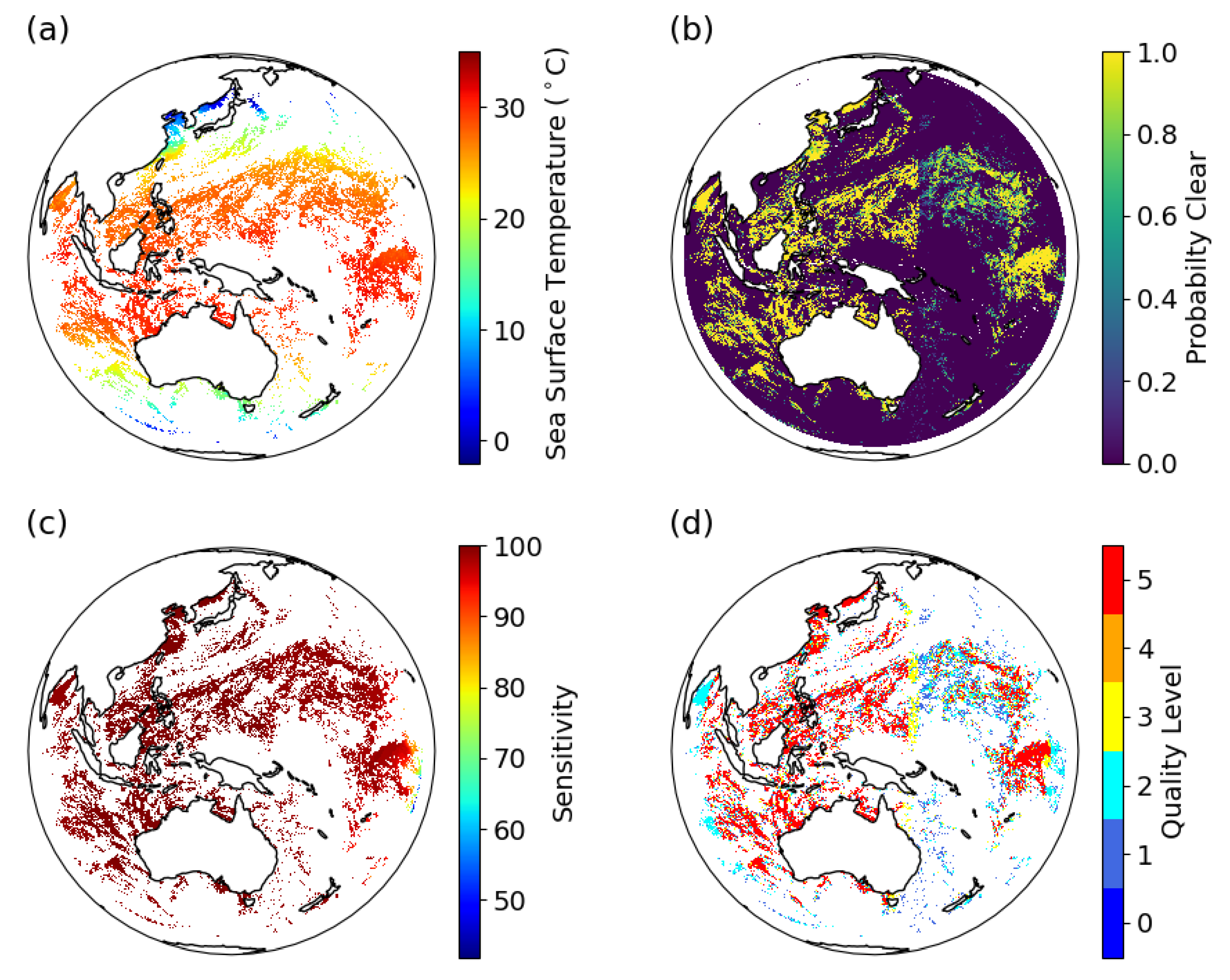
5.1. L2P SST Product

Using the SST retrieval method described in Section 4.1 and Section 4.2, L2P SST products are processed for 2015–2022 every 10 min for Himawari-8. Figure 1a shows skin SST retrieved with our method for one random 10-min instance, for all quality levels. The probability of a pixel being clear derived using the Bayesian approach is shown in Figure 1b. Figure 1c shows sensitivity of retrieved SST to true SST. Sensitivity values are overall greater than 95%, except towards the right edge of the disk, where it falls to approximately 70%. The quality levels assigned to pixels with valid SST values following the process defined in Table 2 are shown in Figure 1d for the same 10 min instance. Towards the edge of the Himawari-8 disk, lower quality levels are generally apparent, mainly reflecting large satellite zenith angles and low sensitivity values. Probability of a pixel being clear and quality level drops off during twilight Figure 1b,d.

An empirical model described in Section 4.2 is applied to the retrieved SST field to estimate uncertainty in the observation. Panel (a) of Figure 2 shows calculated $\mathtt{sses}\_\mathtt{bias}$, panel (b) shows $\mathtt{sses}\_\mathtt{standard}\_\mathtt{deviation}$ and panel (c) $\mathtt{sses}\_\mathtt{count}$ for one 10 min instance L2P SST, based on the model. Large biases are apparent towards the edge of the disk and cloud boundaries. Typically, bias is less than 0.4 K in the tropical regions, whereas the standard deviation is about 0.4–0.6 K. Higher values of biases and standard deviation indicate lower values of quality level (ref Figure 1d).

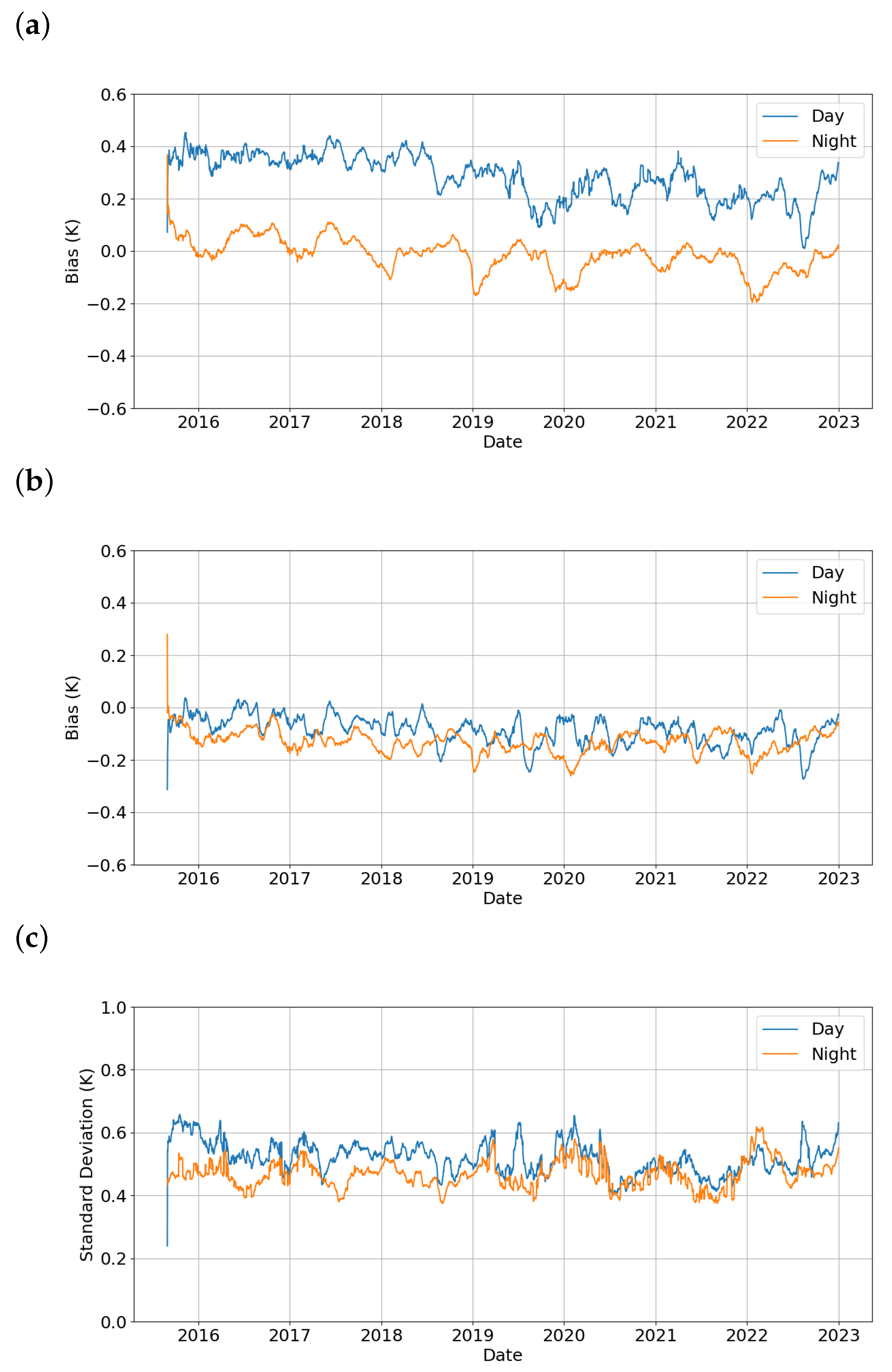
5.2. Coverage and Bias for L2P SST

5.2.1. Temporal and Spatial Bias

Figure 3 shows the L2P validation of SST before and after compensation by subtracting sses_bias, as defined by the presented bias model. The figures represent a full platform lifetime validation, of the parameters $\mathsf{\Delta }\mathrm{SST}$, $\sigma \mathsf{\Delta }\mathrm{SST}$, $\sigma \mathrm{zSST}$, defined as follows.

$$\begin{array}{ccc}\hfill \mathsf{\Delta }\mathrm{SST}& =& {\displaystyle \frac{1}{N}}\sum _{\mathrm{location}}{\mathrm{SST}}_{\mathrm{satellite}}-{\mathrm{SST}}_{\mathrm{in}\mathrm{situ}}\hfill \\ \hfill {\left(\sigma \mathsf{\Delta }\mathrm{SST}\right)}^2& =& {\displaystyle \frac{1}{N}}\sum _{\mathrm{location}}{\left({\mathrm{SST}}_{\mathrm{satellite}}-{\mathrm{SST}}_{\mathrm{in}\mathrm{situ}}-\mathsf{\Delta }\mathrm{SST}\right)}^2\hfill \\ \hfill \mathrm{zSST}& =& {\displaystyle \frac{1}{N}}\sum _{\mathrm{location}}{\displaystyle \frac{{\mathrm{SST}}_{\mathrm{satellite}}-{\mathrm{SST}}_{\mathrm{in}\mathrm{situ}}}{\sigma }}\hfill \\ \hfill {\left(\sigma \mathrm{zSST}\right)}^2& =& {\displaystyle \frac{1}{N}}\sum _{\mathrm{location}}{\left({\displaystyle \frac{{\mathrm{SST}}_{satellite}-{\mathrm{SST}}_{\mathrm{in}\mathrm{situ}}}{\sigma }}-\mathrm{zSST}\right)}^2\hfill \end{array}$$

(22)

Figure 3a clearly shows daytime SST biased positive in the mid-latitudes and tropics, trending warmer closer to the equator. The northern polar latitudes are biased cold, while the south is mainly unbiased, except at high southern latitudes. At night, the tropics remain warm, and all of the southern regions are biased cold, with mid-latitudes close to unbiased. The bias is partially compensated for during the day in the northern hemisphere but overcompensates in the southern hemisphere. The variability, $\sigma \mathsf{\Delta }\mathrm{SST}$, is typically greater in the southern hemisphere and remains unaffected by the bias model (Figure 4), which suggests that the bias correction strategy is not interfering with the independence of measurements. $\sigma \mathrm{zSST}$, which is nominally 1 when the sses_standard_deviation is well chosen, which suggests that while a reasonable estimation is made at night, it is slightly underestimated in the day, and towards edges of the disk (Figure 5).

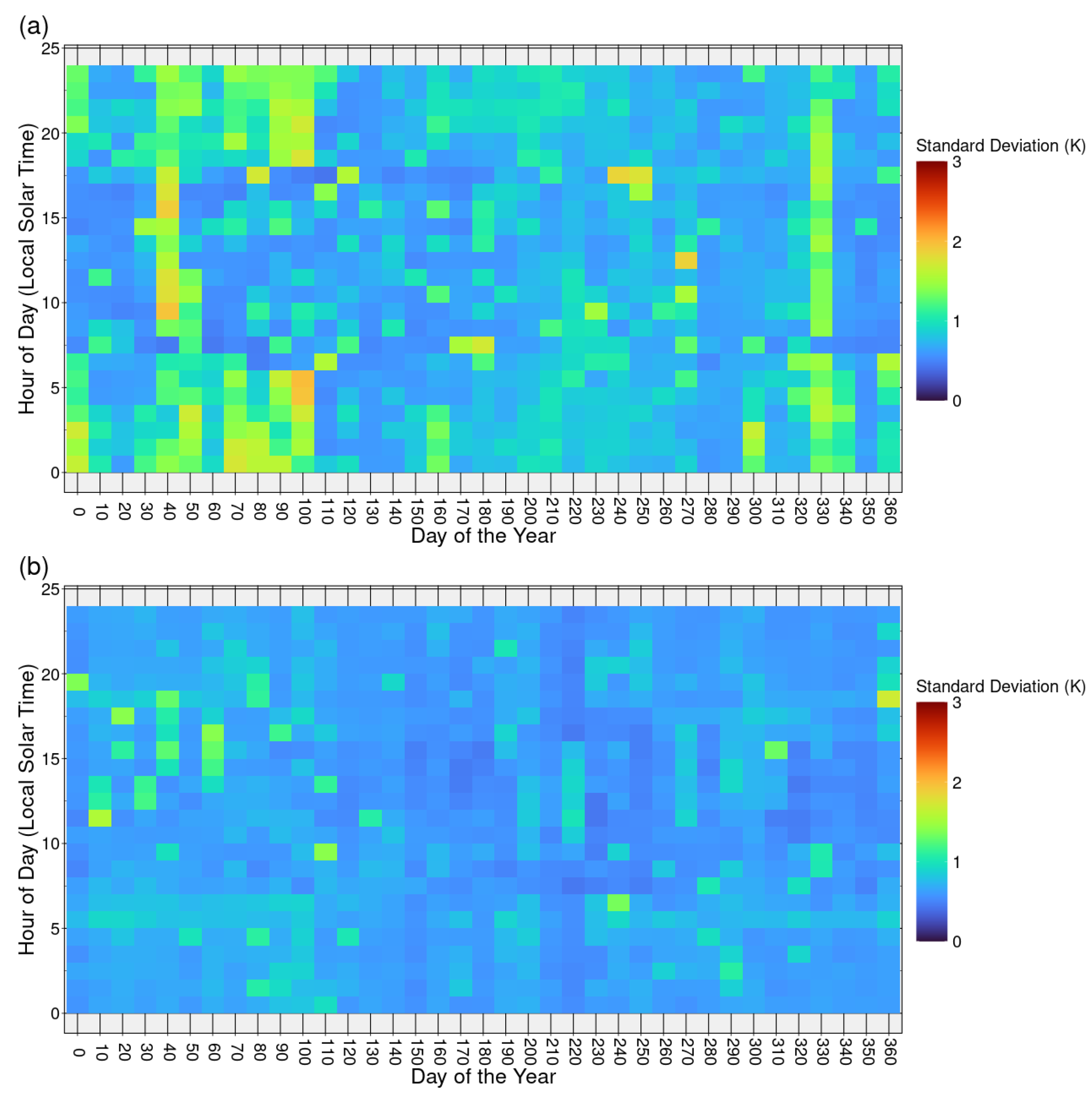
5.2.2. Annual and Diurnal Bias

Figure 6 shows overall bias per hemisphere as a function of time of year and local solar time. Typically, there are negative biases during the night, and positive biases before sunrise and after sunset in summer, with neutral behaviour dominating the northern hemisphere summer. There is no evidence of seasonal hemisphere-wide diurnal signature developing during daytime hours, which is not unexpected, since true diurnal signals would be limited to relatively small well defined geographical regions, and might be expected to be not present on the hemispheric scale shown. Variability (Figure 7) is typically larger in the northern winter than in summer, is larger at night, and relatively lower in the south, which also has a higher consistency compared to the north. $\sigma \mathrm{zSST}$ (Figure 8) is typically high during the northern winter, and slightly lower in the day in both hemispheres. These results demonstrate that the SSES model used has some shortcomings, which reflect the inability of the bias model to functionally reflect the dependencies to temporal parametrisation, and the representativeness of the match-up database that determined the model parameters. The overall negative background bias, with strong positive biases in the vicinity of sunrise/sunset, speaks to the inability to properly fit the time of day dependencies. There are also clear differences in the match-up density that drives these models differently between the hemispheres—the northern hemisphere away from the sunrise/set tends to be relatively neutral compared to the southern hemisphere. This is a focus of ongoing investigation and improvement.

5.2.3. Validation of Full Disk L2P SSTs

Figure 9 shows the monthly validation of L2P SSTs for the entire Himawari-8 platform lifetime, September 2015–December 2022, against iQuam drifting buoys and tropical moorings for QL 3 and above under well mixed conditions. Matchup thresholds used were <10 km distance and $\pm 6$ h time difference. The blue and green lines denote statistics for the northern part of the disk for day and night, respectively, and orange and red lines denote statistics for the southern part of the disk for day and night, respectively. The left-hand side panels show uncorrected mean bias (upper panel) and standard deviation (lower panel), while right-hand panels show results for bias-corrected mean and standard deviation. The bias correction pushes the mean from warmer ($0.3/0.4$ K) to colder ($-0.08/0.01$ K) for daytime for south/north part of the disk, showing more variability over north than south. For night, mean bias is $-0.05$ K for south and $-0.03$ K for north, for uncorrected bias conditions. After bias correction, mean bias is $-0.15$ K for north and $-0.12$ K for south part of the disk. Negative values likely arise due to the bias correction being applied to the skin and we are correcting for the skin effect using $0.2$ m depth typical of drifting buoys data. The standard deviation is between $0.4$ K to $0.7$ K for both cases, before and after bias correction. Both the north and south sides of the disk show lower mean and standard deviation values towards the end years of the lifetime of the platform for both day and night scenarios.

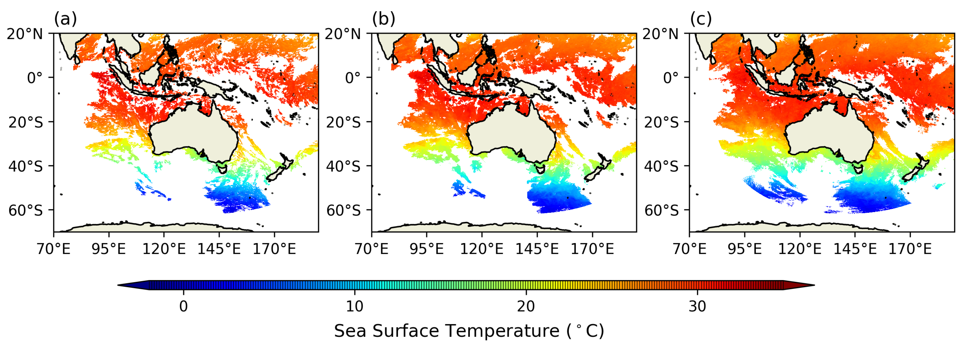
5.3. L3C SST Product

Figure 10 shows composite products for different time scenarios. Panel (a) shows SST data coverage from a 1 h composite, panel (b) shows SST data coverage from a four-hourly composite and panel (c) shows SST data coverage for composition over one night. The progression demonstrates clearly areas near moving clouds that are filled with additional observations due to spatial and temporal proximity in the merging process over the time period of the merge. Generally, the data coverage for L3C-1 h within the IMOS domain is approximately $22\%$, while L3C-04 h has a coverage of about $32\%$. On average, the night composite data spans $47\%$ of the IMOS domain.

The monthly statistics for 1 h and 4 h SST composite products on the IMOS domain for the period September 2015 to December 2022 are shown in Figure 11 and Figure 12, when compared with drifting buoys and tropical moorings from iQuam under well mixed conditions. The upper panels show mean bias and the lower panels show the standard deviation for uncorrected and bias-corrected SSTs. The blue line denotes statistics for the day, and the orange line denotes statistics for the night. With the bias correction, 1 h SST products show a colder bias of about $-0.13$ K and standard deviation $0.45$ K for night (Figure 11). The four-hourly SST product shows similar results with bias-corrected mean bias $-0.1$ K and standard deviation of $0.4$ K for night (Figure 12). Figure 13 shows statistics for L3C 1-night SST product when compared with drifting buoys and tropical moorings from iQuam. Mean is shown in the upper panel, while the standard deviation is shown in the bottom panel of Figure 13 for QL 3 and above. The brown line in this figure denotes statistics calculated with uncorrected SSTs, while the cyan line denotes statistics for bias-corrected SSTs. On average, the mean bias is about $-0.22$ K, which is a colder bias than the mean for uncorrected SSTs ($-0.11$ K). The standard deviation is about $0.48$ K for both cases.

The L3C-1hour SST products are available from the National Computational Infrastructure (NCI) Thematic Real-time Environmental Distributed Data Services (THREDDS) server (https://thredds.nci.org.au/thredds/catalog/qm43/ghrsst/v02.0fv02/Continental/L3C-01hour/ABOM-L3C_GHRSST-SSTskin-AHI_H08/catalog.html, accessed on 6 September 2024) and Australian Ocean Data Network (AODN) (https://thredds.aodn.org.au/thredds/catalog/IMOS/SRS/SST/ghrsst/L3C-1h/h08/catalog.html, accessed on 6 September 2024). L3C-04hour SST products are available at NCI (https://thredds.nci.org.au/thredds/catalog/qm43/ghrsst/v02.0fv02/Continental/L3C-04hour/ABOM-L3C_GHRSST-SSTskin-AHI_H08/catalog.html, accessed on 6 September 2024) and AODN (https://thredds.aodn.org.au/thredds/catalog/IMOS/SRS/SST/ghrsst/L3C-4h/catalog.html, accessed on 6 September 2024). Daily L3C-01day night files are available at NCI (https://thredds.nci.org.au/thredds/catalog/qm43/ghrsst/v02.0fv02/Continental/L3C-01day/night/ABOM-L3C_GHRSST-SSTskin-AHI_H08/catalog.html, accessed on 6 September 2024) and AODN (https://thredds.aodn.org.au/thredds/catalog/IMOS/SRS/SST/ghrsst/L3C-1d/ngt/h08/catalog.html, accessed on 6 September 2024).

6. Application of Himawari-8 SSTs

The Bureau started producing MultiSensor Level 3 super-collated (L3S) SST products on the IMOS 0.02 degree grid [7] by compositing available data from AVHRR sensors on National Oceanic and Atmospheric Administration (NOAA) Polar-orbiting satellites, NOAA-18 and NOAA-19, MetOpB and the Visible Infrared Imaging Radiometer Suite (VIIRS) sensors on Suomi National Polar-orbiting Partnership (SNPP) and NOAA-20 satellites in real-time from October 2018 [9]. These SST products were used until May 2024 for coral heat stress monitoring with the Bureau’s NextGen ReefTemp system [44], and are used by IMOS OceanCurrent (https://oceancurrent.aodn.org.au/, accessed on 6 September 2024) to monitor thermal stress and marine heatwaves. To achieve L3S SST products with fewer spatial data gaps, we composited Himawari-8 night L3C data with the current polar-orbiter-specific operational MultiSensor L3S product using the compositing method described in [9]. The resultant GeoPolar MultiSensor L3S is produced using all available data from AVHRR sensors on polar-orbiters MetOp-B and MetOp-C, VIIRS sensors on Suomi NPP and NOAA-20, and the AHI sensor on Geostationary satellite Himawari-8. The product is available for every night from 1 September 2015 to 12 December 2022.

Figure 14a shows the SST data coverage from the current MultiSensor L3S SST product, which is a composition of data from NOAA-18, MetOpB, SNPP and NOAA-20, while Figure 14b shows SST data coverage from the new GeoPolar MultiSensor L3S SST product which is a composition of data from Himawari-8, MetOpB, SNPP and NOAA-20 for 15 March 2020. As demonstrated here, the GeoPolar MultiSensor L3S SST product has better data coverage compared to the current MultiSensor L3S. On average, the GeoPolar MultiSensor L3S SST product has 20% more data available on the IMOS domain than the regular MultiSensor L3S SST product.

The GeoPolar MultiSensor L3S SST products are available from the NCI THREDDS server (https://thredds.nci.org.au/thredds/catalog/qm43/ghrsst/v02.0fv02/Continental/L3S-01day/night/catalog.html, accessed on 6 September 2024) and AODN (https://thredds.aodn.org.au/thredds/catalog/IMOS/SRS/SST/ghrsst/L3SGM-1d/ngt/catalog.html, accessed on 6 September 2024). The new GeoPolar MultiSensor L3S daily night product is expected to provide better input for Reeftemp NextGen and IMOS OceanCurrent, owing to its better data coverage. With the enhanced spatial data coverage, the GeoPolar MultiSensor L3S product also will help with better monitoring of thermal stress and marine heatwave ocean conditions and facilitate the study of ocean temperature trends.

7. Discussion and Conclusions

Infrared imagery from the AHI sensor on the Himawari-8 satellite is used to retrieve skin SST. The method that the University of Reading developed to derive ESA CCI SST Climate Data Records version 2 from infrared sensors on polar-orbiting satellites was modified and used for the geostationary satellite Himawari-8. Radiative transfer model RTTOV 12.3 was used to simulate top-of-atmosphere radiances from brightness temperatures (BTs). Optimal Estimation was further used to calculate SSTs. Five channels of Himawari-8, $0.64$, $0.86$, $3.9$, $10.4$, and $12.4 \mathsf{\mu }\mathrm{m}$ are used for spectral observations. The channel $3.9 \mathsf{\mu }\mathrm{m}$ was used for only night-time retrievals. The Bureau’s NWP model ACCESS-G analysis and forecast data were used as atmospheric and surface state data. OSTIA L4 ice concentration was used for ice masking and the GAMSSA SST analysis was used as background SST.

A Bayesian approach was used to determine cloud-free regions in the SST retrieval process, where satellite observations and prior knowledge of the surface conditions were used to estimate clear-sky probabilities. The Bayesian approach significantly reduces the occurrence of both missed cloud and false detection of clouds [18]. However, it might not work properly in some specific situations like observations of regions with low-level fog or night-time observations of regions covered with sea ice.

The Bayesian method used in this study for cloud detection did not account for the effect of aerosols. Integrating tropospheric aerosols in the Bayesian cloud detection method may be helpful with some specific SST measurements.

The SSES bias model that the Bureau developed for AVHRR polar orbiters that were acquired through direct reception was applied to Himawari-8. This is an empirical model based on match-ups with in situ SST data. Due to the increase in the frequency of match-up events, a smaller time period was able to be used. A rolling 30-day window was used to define the model parameters, which were re-evaluated every day. For appropriate and representative matchups, we used thresholds of 2 km distance and ±6 h time difference between satellite and in situ observations in well-mixed conditions. Satellite zenith angle, solar zenith angle and quality level of each satellite observation, and geographic coordinates (latitude, longitude, and time of the observation) are used to define bias and standard deviation per pixel. As has been demonstrated, the model has shown some skill in bias correction, although there needs to be further investigation in areas where the original use in polar orbiters differs from geostationary use. This includes investigating and accounting for possible diurnal variability, behaviour around sunrise and sunset, the relationship to the probability of cloud clearance, and the considerable increase in spatial coverage, all of which have been shown to exhibit non-zero bias in the existing model.

The monthly statistics for comparisons of Himawari-8 L2P skin SST against iQuam in situ SST, corrected for the ocean cool-skin under well-mixed conditions, showed mean bias of 0.3–0.4 K for daytime and $-0.2$ K for night-time, for the uncorrected bias case. After bias correction, the mean bias is $-0.04$ K for daytime and $-0.14$ K for night-time. A night-time negative bias is anticipated during high winds, as we are validating skin SST. However, this effect may have been counteracted by diurnal warming during the daytime under conditions of high solar insolation and low winds. The standard deviation is between 0.4 and 0.7 K for both uncorrected and bias-corrected cases. Five years (2016–2020) of the Bureau’s IMOS Himawari-8 L2P skin SST data were validated against shipborne radiometer skin SST measurements obtained from the Infrared SST Autonomous Radiometer (ISAR) onboard research vessel RV Investigator in the study of [45]. They found the daytime mean and median biases are both $-0.12$ K, with an SD/RSD of $0.47/0.31$ K, and night-time mean/median bias of $-0.04/0.03$ K, and an SD/RSD of $0.37/0.24$ K. The negative biases reported in [45] are consistent with our validation results.

The JAXA operationally retrieved Himawari-8 SST from $10.4$, $11.2$, and 8.6 μm channels using a quasi-physical SST algorithm and cloud screening based on a Bayesian cloud detection method. Those JAXA Himawari-8 SSTs on the full disk were compared with drifting buoys and tropical moorings for June to September 2015 in [3]. They found mean bias between $0.044$ and $-0.14$ K during daytime and between $-0.14$ and $-0.24$ K during night-time and twilight. The standard deviation values were between $0.38$ and $0.62$ K during the day where satellite zenith angles were less than 60°, and more than $0.75$ K at night where satellite zenith angles were greater than 60°. When JAXA Himawari-8 skin SST were compared with ISAR skin SST in the Australian region for 2016 and 2017, a mean bias of 0.09 K and standard deviation of 0.30 K were reported [46]. The study [46] found significant differences between skin and bulk SST measurements of maximum value 2.23 K under conditions of high diurnal warming and demonstrated that Himawari-8 AHI skin SST can accurately measure diurnal warming events. Although [45,46] undertook similar comparisons for Himawari-8 SST from JAXA and the Bureau against ISAR, respectively, ref. [46] comparison showed better agreement, which can be attributed to a more stringent choice for their match-up selection—quality Level 5 satellite retrievals far from the edge of suspected cloud boundaries. Statistics can be improved by applying a very harsh cloud mask for the Bureau’s SST product but that would affect the data coverage. Our users, such as fishers, prefer maximum possible data coverage so the trade-off might not be what we aim for if the coverage is then very low in some regions.

The NOAA Centre for Satellite Applications and Research (STAR) operationally produced Himawari-8 SST products using NOAA’s Advanced Clear-Sky Processor for Oceans (ACSPO) SST system and monitored product performance against in situ data in the NOAA SST Quality Monitor (SQUAM, https://www.star.nesdis.noaa.gov/sod/sst/squam, accessed on 3 September 2024). They produce sub-skin SST using regression algorithms. The comparison of the NOAA ACSPO Himawari-8 SST product against drifters and tropical moorings for June to September 2015 showed a bias within ±0.2 K and standard deviation within 0.46 K [4]. A mean bias of 0.18 K with standard deviation of 0.53 K was reported for the comparison of NOAA ACSPO Himawari-8 SST product with tropical moorings and buoys in the Australian Great Barrier Reef region for August to October 2015 [47]. Contrary to their positive biases for sub-skin SSTs, our validation results for L2P skin SST show negative biases similar to JAXA skin SST products.

It is important to note that retrieval error standard deviation can be traded off against SST sensitivity [1]. The SST sensitivity is the amount of change in retrieved SST for a given change in the true SST (background SST). Earlier studies have demonstrated that low sensitivity algorithms can have better standard deviation if they are over-fitted to training data (e.g., [48]). Our retrieved SST showed higher values of sensitivity in general (ref. Figure 1c). For QL $\ge 3$, at least 95 % sensitivity was achieved in our SST retrieval process.

The data were composited for 1 h, 4 h and daily night scenarios and further all composite products were projected on the IMOS standard 0.02 degree grid. All Himawari-8 data were reprocessed back to 2015 and made available through the Australian Ocean Data Network (AODN, https://portal.aodn.org.au, accessed on 3 September 2024) and National Computational Infrastructure (NCI, [49]). All the L3C products were compared with iQuam in situ SSTs and monthly statistics were presented for the entire platform life, September 2015–December 2022, after applying a 0.17 K adjustment for the cool-skin and under well-mixed ocean conditions. The 1 h L3C skin SST showed a bias of −0.13 K and a standard deviation of 0.45 K for night. The four-hourly SST showed a mean bias of −0.1 K and a standard deviation in excess of 0.4 K. The 1-day night skin SST showed a mean bias of −0.22 K and a standard deviation of 0.48 K. The availability of enhanced data coverage with the addition of Himawari-8 data to existent Level 2 and 3 SST products will help with many applications such as IMOS OceanCurrent (https://oceancurrent.aodn.org.au/, accessed on 6 September 2024), and investigations into marine thermal stress, marine heatwaves and ocean upwelling in near-coastal regions.

It is believed there is potential for improvement in these newly developed Himawari-8 SST products. Future work will be focused along two major lines, improvement in SST retrieval process and development of the geostationary satellite specific bias model. The University of Reading has developed ESA SST CCI version 3 code and processed skin SSTs from infrared radiometers on polar orbiters (AVHRR, ATSR, SLSTR) to derive Level 2, Level 3 and Level 4 climate data records [50], which improves the representation of radiative effects of tropospheric aerosols for cloud detection and SST retrieval, reducing the previous few-tenth degrees Celsius cold biases associated with desert dust aerosols. We will be modifying this new version of the code to retrieve skin SSTs from Himawari-8 and Himawari-9. We will also modify the Bureau’s SSES model to better address diurnal discrimination as well as a better representation of the matchup dataset over two hemispheres. With the newly developed code, we plan to process Himawari-9 in near real time by June 2025 and reprocess the entire skin SST data record from Himawari-8 and Himawari-9.

References

1. Merchant, C.J.; Embury, O.; Bulgin, C.E.; Block, T.; Corlett, G.K.; Fiedler, E.; Good, S.A.; Mittaz, J.; Rayner, N.A.; Berry, D.; et al. Satellite-based time-series of sea-surface temperature since 1981 for climate applications. Sci. Data 2019, 6, 223. [Google Scholar] [CrossRef] [PubMed]
2. Bessho, K.; Date, K.; Hayashi, M.; Ikeda, A.; Imai, T.; Inoue, H.; Kumagai, Y.; Miyakawa, T.; Murata, H.; Ohno, T.; et al. An Introduction to Himawari-8/9—Japan’s New-Generation Geostationary Meteorological Satellites. J. Meteorol. Soc. Jpn. Ser. II 2016, 94, 151–183. [Google Scholar] [CrossRef]
3. Kurihara, Y.; Murakami, H.; Kachi, M. Sea Surface Temperature from the New Japanese Geostationary Meteorological Himawari-8 Satellite. Geophys. Res. Lett. 2016, 43, 1234–1240. [Google Scholar] [CrossRef]
4. Kramar, M.; Ignatov, A.; Petrenko, B.; Kihai, Y.; Dash, P. Near real time SST retrievals from Himawari-8 at NOAA using ACSPO system. Ocean. Sens. Monit. VIII 2016, 9827, 149–159. [Google Scholar] [CrossRef]
5. Heidinger, A.K. ABI cloud height. In Algorithm Theoretical Basis Document; NOAA NESDIS Center for Satellite Applications and Research: Silver Spring, MD, USA, 2013; 77p. Available online: https://www.star.nesdis.noaa.gov/goesr/docs/ATBD/Cloud_Height.pdf (accessed on 3 September 2024).
6. Huang, Y.; Siems, S.; Manton, M.; Protat, A.; Majewski, L.; Nguyen, H. Evaluating Himawari-8 Cloud Products Using Shipborne and CALIPSO Observations: Cloud-Top Height and Cloud-Top Temperature. J. Atmos. Ocean. Technol. 2019, 36, 2327–2347. [Google Scholar] [CrossRef]
7. GHRSST Science Team. The Recommended GHRSST Data Specification (GDS) 2.0, Document Revision 4; GHRSST Science Team: Montréal, QC, USA, 2010; p. 123. [Google Scholar] [CrossRef]
8. Griffin, C.; Beggs, H.; Majewski, L. GHRSST Compliant AVHRR SST Products over the Australian Region Version 1; Technical Report; Bureau of Meteorology: Melbourne, Australia, 2017; p. 151. [Google Scholar]
9. Govekar, P.D.; Griffin, C.; Beggs, H. Multi-sensor Sea Surface Temperature products from the Australian Bureau of Meteorology. Remote. Sens. 2022, 14, 3785. [Google Scholar] [CrossRef]
10. Saunders, R.W.; Hocking, J.; Turner, E.; Rayer, P.; Rundle, D.; Brunel, P.; Vidot, J.; Roquet, P.; Matricardi, M.; Geer, A.; et al. An update on the RTTOV fast radiative transfer model (currently at version 12). Int. J. Remote. Sens. 2018, 11, 123–150. [Google Scholar] [CrossRef]
11. Minnett, P.; Kaiser-Weiss, A.K. Near-Surface Oceanic Temperature Gradients; Discussion Document; Group for High Resolution Sea-Surface Temperature: Leicester, UK, 2012; p. 7. Available online: https://www.ghrsst.org/wp-content/uploads/2021/04/SSTDefinitionsDiscussion.pdf (accessed on 3 September 2024).
12. Merchant, C.J.; Harris, A.R.; Maturi, E.; MacCallum, S. Probabilistic physically-based cloud screening of satellite infra-red imagery for operational sea surface temperature retrieval. Q. J. R. Meteorol. Soc. 2005, 131, 2735–2755. [Google Scholar] [CrossRef]
13. Bulgin, C.E.; Mittaz, J.P.D.; Embury, O.; Eastwood, S.; Merchant, C.J. Bayesian cloud detection for 37 Years of Advanced Very High Resolution Radiometer (AVHRR) Global Area Coverage (GAC) data. Remote Sens. 2018, 10, 97. [Google Scholar] [CrossRef]
14. Merchant, C.J.; Borgne, P.L.; Roquet, H.; Legendre, G. Extended optimal estimation techniques for sea surface temperature from the Spinning Enhanced Visible and Infra-Red Imager (SEVIRI). Remote Sens. Environ. 2013, 131, 287–297. [Google Scholar] [CrossRef]
15. Andersson, E.; Haseler, J.; Undén, P.; Courtier, P.; Kelly, G.; Vasiljevic, D.; Brankovic, C.; Gaffard, C.; Hollingsworth, A.; Jakob, C.; et al. The ECMWF implementation of three-dimensional variational assimilation (3D-Var). III: Experimental results. Q. J. Roy. Meteor. Soc 1998, 124, 1831–1860. [Google Scholar] [CrossRef]
16. Eyre, J.R.; Kelly, G.A.; McNally, A.P.; Andersson, E.; Persson, A. Assimilation of TOVS radiance information through one-dimensional variational analysis. Q. J. R. Meteorol. Soc. 1993, 119, 1427–1463. [Google Scholar] [CrossRef]
17. Li, J.; Wolf, W.; Menzel, W.P.; Zhang, W.; Huang, H.; Achtor, T.H. Global soundings of the atmosphere from ATOVS measurements: The algorithm and validation. J. Appl. Meteorol. 2000, 39, 1248–1268. [Google Scholar] [CrossRef]
18. Embury, O.; Merchant, C.J.; Corlett, G.K. A reprocessing for climate of sea surface temperature from the along-track scanning radiometers: Initial validation, accounting for skin and diurnal variability effects. Remote Sens. Environ. 2012, 116, 62–78. [Google Scholar] [CrossRef]
19. Saunders, R.W. An automated scheme for the removal of cloud contamination from AVHRR radiances over Western Europe. Int. J. Remote Sens. 1986, 7, 867–886. [Google Scholar] [CrossRef]
20. Saunders, R.W.; Kriebel, K.T. An improved method for detecting clear-sky and cloudy radiances from AHRR data. Int. J. Remote Sens. 1988, 9, 123–150. [Google Scholar] [CrossRef]
21. Rossow, W.B.; Garder, L.C. Cloud Detection Using Satellite Measurements of Infrared and Visible Radiances for ISCCP. J. Clim. 1993, 12, 2341–2369. [Google Scholar] [CrossRef]
22. Frey, R.; Ackerman, S.; Liu, Y.; Strabala, K.; Zhang, H.; Key, J.; Wang, X. Cloud Detection with MODIS. Part I: Improvements in the MODIS Cloud Mask for Collection 5. J. Ofatmospheric Ocean. Technol. 2008, 25, 1057–1072. [Google Scholar] [CrossRef]
23. Rodgers, C.D. Inverse Methods for Atmospheric Sounding: Theory and Practice; World Scientific: Singapore, 2000; ISBN 139789810227401. [Google Scholar] [CrossRef]
24. Merchant, C.J.; Borgne, P.L.; Roquet, H.; Marsouin, A. Sea surface temperature from a geostationary satellite by optimal estimation. Remote Sens. Environ. 2009, 113, 445–457. [Google Scholar] [CrossRef]
25. Merchant, C.J.; Le Borgne, P.; Marsouin, A.; Roquet, H. Optimal estimation of sea surface temperature from split-window observations. Remote Sens. Environ. 2008, 112, 2469–2484. [Google Scholar] [CrossRef]
26. Bureau of Meteorology (2022): Bureau of Meteorology Satellite Archive (Collection) NCI Australia. Available online: https://geonetwork.nci.org.au/geonetwork/srv/eng/catalog.search#/metadata/f9367_4020_5456_5573 (accessed on 6 September 2024).
27. Zhong, A.; Beggs, H. Operational Implementation of Global Australian Multi-Sensor Sea Surface Temperature Analysis. Anal. Predict. Oper. Bull. Bur. Meteorol. Melb. Aust. 2008, 77, 43. [Google Scholar]
28. Beggs, H.; Qi, L.; Govekar, P.; Griffin, C. Ingesting VIIRS SST into the Bureau of Meteorology’s Operational SST Analyses. In Proceedings of the GHRSST XXI Science Team Meeting, Virtual, 1–4 June 2020; Virtual Meeting Hosted by EUMETSAT. pp. 104–110. [Google Scholar] [CrossRef]
29. Puri, K.; Dietachmayer, G.; Steinle, P.; Dix, M.; Rikus, L.; Logan, L.; Naughton, M.; Tingwell, C.; Xiao, Y.; Barras, V.; et al. Implementation of the initial ACCESS numerical weather prediction system. Aust. Meteorol. Oceanogr. J. 2013, 63, 265–284. [Google Scholar] [CrossRef]
30. National Operational Centre Operations Bulletin Number 125 (2019), APS3 Upgrade of the ACCESS-G/GE Numerical Weather Prediction System. Available online: http://reg.bom.gov.au/australia/charts/bulletins/opsbull_G3GE3_external_v3.pdf (accessed on 27 May 2024).
31. National Meteorological and Oceanographic Centre Operations Bulletin Number 93 (2012), APS1 Upgrade of the ACCESS-G Numerical Weather Prediction System. Available online: http://www.bom.gov.au/australia/charts/bulletins/apob93.pdf (accessed on 27 May 2024).
32. Bureau National Operations Centre Operations Bulletin Number 105 (2016), APS2 Upgrade to the ACCESS-G Numerical Weather Prediction System. Available online: http://www.bom.gov.au/australia/charts/bulletins/APOB105.pdf (accessed on 27 May 2024).
33. Good, S.; Fiedler, E.; Mao, C.; Martin, M.J.; Maycock, A.; Reid, R.; Roberts-Jones, J.; Searle, T.; Waters, J.; While, J.; et al. The Current Configuration of the OSTIA System for Operational Production of Foundation Sea Surface Temperature and Ice Concentration Analyses. Remote Sens. 2020, 12, 720. [Google Scholar] [CrossRef]
34. Merchant, C.J.; Harris, A.R.; Roquet, H.; Borgne, P.L. Retrieval characteristics of non-linear sea surface temperature from the Advanced Very High Resolution Radiometer. Geophys. Res. Lett. 2009, 36, L17604. [Google Scholar] [CrossRef]
35. Gentemann, C.L.; Minnett, P.J.; Borgne, P.L.; Merchant, C.J. Multi-satellite measurements of large diurnal warming events. Geophys. Res. Lett. 2008, 35, L22602. [Google Scholar] [CrossRef]
36. Cayula, J.F.; May, D.; McKenzie, B.; Olszewski, D.; Willis, K. Reliability estimates for real-time sea surface temperature. Sea Technol. 2004, 45, 67–74. [Google Scholar]
37. Kilpatrick, K.A.; Podestá, G.; Walsh, S.; Williams, E.; Halliwell, V.; Szczodrak, M.; Brown, O.B.; Minnett, P.J.; Evans, R. A decade of sea surface temperature from MODIS. Remote Sens. Environ. 2015, 165, 27–41. [Google Scholar] [CrossRef]
38. Petrenko, B.; Ignatov, A.; Kihai, Y.; Dash, P. Sensor-specific error statistics for SST in the Advanced Clear-Sky Processor for Ocean. J. Atmos. Ocean. Technol. 2016, 33, 345–359. [Google Scholar] [CrossRef]
39. Donlon, C.; Minnett, P.J.; Gentemann, C.; Nightingale, T.J.; Barton, I.; Ward, B.; Murray, M.J. Toward improved validation of satellite sea surface skin temperature measurements for climate research. J. Clim. 2002, 15, 353–369. [Google Scholar] [CrossRef]
40. Rayner, N.; Brohan, P.; Parker, D.E.; Folland, C.K.; Kennedy, J.J.; Ansell, M.V.T.J.; Tett, S.F.B. Improved analyses of changes and uncertainties in sea surface temperature measured in situ since the mid-nineteenth century: The HadSST2 dataset. J. Clim. 2006, 19, 446–469. [Google Scholar] [CrossRef]
41. Xu, F.; Ignatov, A. Evaluation of in situ sea surface temperatures for use in the calibration and validation of satellite retrievals. J. Geophys. Res. 2010, 115, C09022. [Google Scholar] [CrossRef]
42. Xu, F.; Ignatov, A. in situ SST quality monitor (iQuam). J. Atmos. Ocean. Technol. 2014, 31, 164–180. [Google Scholar] [CrossRef]
43. Xu, F.; Ignatov, A. Error characterization in iQuam SSTs using triple collocations with satellite measurements. Geophys. Res. Lett. 2016, 43, 10826–10834. [Google Scholar] [CrossRef]
44. Garde, L.; Spillman, M.C.; Heron, S.; Beeden, R. ReefTemp Next Generation: A New Operational System for Monitoring Reef Thermal Stress. J. Oper. Oceanogr. 2014, 7, 21–33. [Google Scholar] [CrossRef]
45. Zhang, H.; Beggs, H.; Griffin, C.; Govekar, P. Validation of Himawari-8 Sea Surface Temperature retrievals using Infrared SST Autonomous Radiometer Measurements. Remote Sens. 2023, 15, 2841. [Google Scholar] [CrossRef]
46. Yang, M.; Guan, L.; Beggs, H.; Morgan, N.; Kurihara, Y.; Kachi, M. Comparison of Himawari-8 AHI SST with Shipboard Skin SST Measurements in the Australian Region. Remote Sens. 2020, 12, 1237. [Google Scholar] [CrossRef]
47. Ditri, A.L.; Minnett, P.J.; Liu, Y.; Kilpatrick, K.; Kumar, A. The Accuracies of Himawari-8 and MTSAT-2 Sea-Surface Temperatures in the Tropical Western Pacific Ocean. Remote Sens. 2018, 10, 212. [Google Scholar] [CrossRef]
48. Petrenko, B.; Ignatov, A.; Shabanov, N.; Kihal, Y. Development and evaluation of SST algorithms for GOES-R ABI using MSG SEVIRI as a proxy. Remote Sens. Environ. 2011, 115, 3647–3658. [Google Scholar] [CrossRef]
49. National Computational Infrastructure (NCI) Australia (2019). Gadi Supercomputer, NCI Australia (Service). Available online: https://nci.org.au (accessed on 6 September 2024).
50. Embury, O.; Merchant, C.J.; Good, S.A.; Rayner, N.A.; Høyer, J.L.; Atkinson, C.; Block, T.; Alerskans, E.; Pearson, K.J.; Worsfold, M.; et al. Satellite-based time-series of sea-surface temperature since 1980 for climate applications. Sci. Data 2024, 11, 326. [Google Scholar] [CrossRef]
51. IMOS fv02 1-Hour Himawari-8 L3C Data. Available online: https://thredds.aodn.org.au/thredds/catalog/IMOS/SRS/SST/ghrsst/L3C-1h/h08/catalog.html (accessed on 26 March 2024).
52. IMOS fv02 4-Hour Himawari-8 L3C Data. Available online: https://thredds.aodn.org.au/thredds/catalog/IMOS/SRS/SST/ghrsst/L3C-4h/h08/catalog.html (accessed on 26 March 2024).
53. IMOS fv02 1-Day Night Himawari-8 L3C Data. Available online: https://thredds.aodn.org.au/thredds/catalog/IMOS/SRS/SST/ghrsst/L3C-1d/ngt/h08/catalog.html (accessed on 26 March 2024).
54. IMOS fv02 Night GeoPolar MultiSensor L3S Data. Available online: https://thredds.aodn.org.au/thredds/catalog/IMOS/SRS/SST/ghrsst/L3SGM-1d/ngt/catalog.html (accessed on 26 March 2024).
55. Bureau Of Meteorology (2021): Bureau of Meteorology Satellite Observations (Collection). NCI Australia. Available online: https://geonetwork.nci.org.au/geonetwork/srv/eng/catalog.search#/metadata/f3533_2249_9116_3778 (accessed on 5 July 2024).
Figure 1. (a) SST, (b) probability of a pixel being clear, (c) sensitivity, and (d) assigned quality levels for one random L2P on 15 December 2020, 20:00:00 UTC, for all quality levels.
Remotesensing 16 03381 g001
Figure 2. (a) sses _ bias , (b) sses _ standard _ deviation , and (c) sses _ count for one random L2P on 15th December 2020, 20:00:00 UTC.
Remotesensing 16 03381 g002
Figure 3. Full disk spatial coverage Himawari-8 L2P validation against drifting buoys and tropical moorings, September 2015–December 2022, showing the impact of bias correction on day (top) and night (bottom) retrievals, Δ SST . Left—hand panels show variables before bias correction, and right—hand panels after bias correction have been applied to the SST values. The grey region indicates pixels with no data.
Remotesensing 16 03381 g003
Figure 4. Same as Figure 3, for σ Δ SST .
Remotesensing 16 03381 g004
Figure 5. Same as Figure 3, for σ zSST .
Remotesensing 16 03381 g005
Figure 6. Annual and diurnal performance of full disk Himawari-8 L2P validation against drifting buoys and tropical moorings for September 2015–December 2022 for (a) northern and (b) southern part of the disk. The colour indicates mean bias, when bias-corrected SST is compared with drifting buoys and tropical moorings.
Remotesensing 16 03381 g006
Figure 7. Same as Figure 6. Here, the colour indicates standard deviation, when bias-corrected SST compared with drifting buoys and tropical moorings for (a) northern and (b) southern part of the disk.
Remotesensing 16 03381 g007
Figure 8. Same as Figure 6. Here, the colour indicates z s s e s , when bias-corrected SST is compared with drifting buoys and tropical moorings for (a) northern and (b) southern part of the disk.
Remotesensing 16 03381 g008
Figure 9. Full disk Himawari-8 L2P skin SST validation against drifting buoys and tropical moorings, 30-day running statistics, September 2015–December 2022, (a) uncorrected mean, (b) bias-corrected mean, (c) uncorrected standard deviation, and (d) bias-corrected standard deviation, for QL ≥ 3.
Remotesensing 16 03381 g009aRemotesensing 16 03381 g009b
Figure 10. Composite SSTs for (a) 1 h, (b) 4 h and (c) 1 night on the IMOS domain for 15 December 2020.
Remotesensing 16 03381 g010
Figure 11. Monthly statistics for validation of 1-hour L3C skin SST against drifting buoys and tropical moorings for September 2015–December 2022 on the IMOS domain, uncorrected (a) mean and (c) standard deviation, bias-corrected (b) mean and (d) standard deviation, for QL ≥ 3. Daytime validations are shown in blue, and night-time validations in orange.
Remotesensing 16 03381 g011aRemotesensing 16 03381 g011b
Figure 12. Same as Figure 11, for L3C-4hour SSTs.
Remotesensing 16 03381 g012aRemotesensing 16 03381 g012b
Figure 13. Monthly statistics for 1-day Night L3C skin SST validation against drifting buoys and tropical moorings for September 2015–December 2022 for the IMOS domain (a) mean, (b) standard deviation, for QL ≥ 3. The brown line denotes uncorrected data, whereas the cyan line corresponds to bias−corrected data.
Remotesensing 16 03381 g013
Figure 14. SST data coverage from (a) MultiSensor and (b) GeoPolar MultiSensor L3S SST product on the IMOS domain for 15th December 2020.
Remotesensing 16 03381 g014