Article

Revisiting the 2017 Jiuzhaigou (Sichuan, China) Earthquake: Implications for Slip Inversions Based on InSAR Data

1
Chengdu Institute of Survey and Investigation, Chengdu 610023, China
2
School of Geodesy and Geomatics, Wuhan University, Wuhan 430079, China
*
Author to whom correspondence should be addressed.
Remote Sens. 2024, 16(18), 3406; https://doi.org/10.3390/rs16183406
Submission received: 29 July 2024 / Revised: 19 August 2024 / Accepted: 10 September 2024 / Published: 13 September 2024
(This article belongs to the Special Issue Synthetic Aperture Radar Interferometry Symposium 2024)

Abstract

:
The 2017 Jiuzhaigou earthquake (Ms = 7.0) struck the eastern Tibetan Plateau and caused extensive concern. However, the reported slip models of this earthquake have distinct discrepancies and cannot provide a good fit for GPS data. The Jiuzhaigou earthquake also presents a good opportunity to investigate the question of how to avoid overfitting of InSAR observations for co-seismic slip inversions. To comprehend this shock, we first used pre-seismic satellite optical images to extract a surface trace of the seismogenic fault, which constitutes the northern segment of the Huya Fault. Then, we collected GPS observations as well as to measure the co-seismic displacements. Lastly, joint inversions were carried out to obtain the slip distribution. Our results showed that the released moment was 5.3 × 10¹⁸ N m, equivalent to Mw 6.4 with a rigidity of 30 GPa. The maximum slip at a depth of ~6.8 km reached up to 1.12 m, dominated by left-lateral strike-slip. The largest potential surface rupture occurred in the center of the seismogenic fault with strike- and dip-slip components of 0.4 m and 0.2 m, respectively. Comparison with the focal mechanisms of the 1973 Ms 6.5 earthquake and the 1976 triplet of earthquakes (Mw > 6) on the middle and south segments of the Huya Fault indicated different regional motion and slip mechanisms on the three segments. The distribution of co-seismic landslides had a strong correlation with surface displacements rather than surface rupture.

1. Introduction

On 8 August 2017, an Mw 6.5 earthquake occurred in the Jiuzhaigou Valley, a well-known famous scenic area in Sichuan, China, and aroused wide concern (Figure 1) [1]. This region is located in the eastern margin of the Tibetan Plateau, where the Kunlun Fault terminates. The left-lateral strike-slip Kunlun Fault is a major intracontinental fault system in Southwest China that plays a significant role in accommodating the post-collisional convergence between the Eurasian and Indian plates [2,3]. In 2001, the Mw 7.8 Kokoxili earthquake ruptured the west part of the Kunlun Fault, with a total length over 400 km [4]. The left-lateral slip rate on the central Kunlun Fault is about 10 mm/yr and decreases gradually eastwards [5,6,7,8]. In its easternmost segment, the left-lateral slip mainly transfers into the Longriba, Minjiang, Huya and Tazang Faults, probably resulting in the uplift of the Min Shan [9,10]. The 2017 Jiuzhaigou earthquake occurred in the transfer zone between the left-lateral and reverse slip.
The transfer region is also seismically active in the recent years. The 2017 Jiuzhaigou earthquake is the third strong shock in the past ten years following the 2008 Mw 7.9 Wenchuan and 2013 Mw 6.6 Lushan earthquakes. Based on the spatial distribution of relocated aftershocks, Xu et al. [10] proposed this shock occurred on the northern segment of the Huya Fault. The GCMT and USGS W-phase moment tensor solutions indicate that it is a left-lateral strike-slip event with the epicenter at a depth of ~14 km (Table 1). In 1973, a Ms 6.5 occurred in the southeast of this event with a distance of ~30 km and was also characterized by strike-slip. Three years later, the Songpan earthquake swarm, including three Mw > 6 shocks, ruptured the southern segment of the Huya Fault. Their focal mechanisms showed mainly reverse-slip motion [14], completely different from that of the Jiuzhaigou earthquake. Until now, there has been no report on surface rupture in the 2017 Jiuzhaigou earthquake. However, according to the empirical relationship between rupture length and magnitude [16], an Ms = 7.0 strike-slip earthquake generally produces co-seismic surface rupture.
After this event, several studies reported the slip models of the Jiuzhaigou earthquake [17,18,19,20,21,22,23,24,25,26,27,28,29,30,31,32,33,34,35]. However, these models have distinct discrepancies. Firstly, the peak slip ranges from 0.68 m to 2.6 m, associated with a slip angle increasing from 0° to 54.8°. The maximum slip magnitude is a significant output of slip inversions. If the long-term slip rate is known from geological and geodetic studies, the recurrence period of an earthquake can be obtained based on these two kinds of results [36]. Secondly, Sun et al. [27] claimed that three fault segments ruptured during this event, which is different from the other models. Thirdly, all the published slip models used Sentinel-1A InSAR data, but their degrees of misfit with the observations range from 0.25 cm to 6 cm. In addition, the slip models from joint inversions of GPS and InSAR data [23,34] cannot provide a good fit for GPS data. Given these reasons, it is necessary to inspect the slip models of the Jiuzhaigou earthquake.
In addition, we noticed that there another question on co-seismic slip inversions using InSAR data, which did not attract sufficient attention before: how to avoid overfitting of InSAR observations. The prominent features of InSAR observations have large enough numbers of observations, except for the case of severe de-coherence in the near field, and are without observation errors, although they can be estimated using a 1D covariance function in the non-deforming areas [37]. This question needs to be answered because more and more co-seismic slip distributions are obtained from inversions of InSAR data. The Jiuzhaigou earthquake provides a good opportunity to investigate the question, which is probably one of the reasons for the difference among the published slip models.
In this study, we first reinterpreted the pre- and post-seismic satellite images to identify the seismogenic fault trace and the triggered landslides. Secondly, we collected GPS data from eight sites in the earthquake region, including five from the Beidou Foundation Reinforcement System (BFRS) and two from the Phase II project of the Crustal Movement Observation Network of China (CMONOC), as well as the two InSAR interferograms, to measure the co-seismic displacements. Thirdly, we conducted joint inversions and checkerboard resolution tests to determine the reasonable weight ratio between GPS and InSAR data. Lastly, we discussed implications for the slip inversions with InSAR data and the relationship between landslide distribution and ground displacements.

2. Materials

2.1. The Seismogenic Fault

The northern Huya Fault, where the 2017 Jiuzhaigou earthquake occurred, does not connect to the Kunlun Fault in the current active tectonics map (Figure 1). Relocated aftershocks with a focal mechanism suggest this shock ruptured a northwest-trending strike-slip fault [13]. However, no surface rupture was reported after the post-seismic field investigation, possibly due to the wide distribution of co-seismic landslides (Figure 2a), which are identified through visual interpretation of post-seismic Geoeye-1 satellite images [10]. The epicenter was located almost at the center of the co-seismic landslides, which also had a NW–SE distribution. Most of the landslides occurred in the northwest of the epicenter.
To find out whether there are some pre-existing surface traces of the 2017 Jiuzhaigou earthquake fault, we can revisit the pre-seismic satellite images. Southeast of the epicenter, there is a clear linear feature crossing the Xiongmao Lake on the pre-seismic Google Earth (version 1.3) imagery, suggesting that a fault existed before the earthquake. Figure 2b reveals that, northwest of the lake, the fault is marked by a linear fault trough and beheaded and deflected channels. In contrast, southeast of the lake, the fault is characterized by linear offset ridges and sag pond (Figure 2c). Northwest of the epicenter, the land is marked by offset ridges and a linear valley at Shawu Village, Zhangzha Town (Figure 2d). These features indicate that the fault underwent left-lateral strike-slip motion and was probably active in the late Quaternary. The plausible fault traces extracted from pre-seismic optical images, associated with the relocated aftershock distribution, show a similar linear feature. Based on them, we simplified the surface trace of the seismogenic fault into a line for subsequent modelling.

2.2. GPS Data

After the Jiuzhaigou earthquake occurred, the National Earthquake Infrastructure Service (NEIS) collected GNSS data including both stations from CMONOC and BFRS. In our study region, there are 7 stations in total (Figure 3a). Among them, only 1 station is located on the southwest side of the seismogenic fault. The other 6 stations are on the northeast side. GSWD and SCSP are CMONOC stations (Table 2).
In data processing, we selected the pre-seismic observations of 15 days at the sites, as well as the post-seismic observations of 4 days. The software GAMIT (version 10.5) was adopted to obtain daily loosely constrained parametric solutions [38]. Then we chose some stable stations as reference stations, which were not affected by the Jiuzhaigou event, to obtain the coordinate time series of all 7 stations in a regional reference frame. In the last, we fitted the pre- and post-seismic time series separately and calculated the co-seismic horizontal displacement of each station with the least-squares estimation method.
To obtain a stable regional reference frame in the observation period, we took the following steps: (1) the GPS stations in a distance of 150–350 km from the epicenter were selected as the initial reference sites based on rapid GNSS solutions; (2) a regional reference frame was fixed by using the HELMERT method and the initial reference stations for each observation day; (3) the common stations in the regional reference frames of 19 days were selected as new reference sites to update the reference stations used in the 2nd step; (4) the 2nd and 3rd steps were repeated cyclically to obtain stable reference stations. Table 2 lists the eventual co-seismic horizontal displacements at 7 sites, with the largest value occurring at station SCJZ and measuring up to 1.0 cm; the sites showed distinct sinistral fault motion (Figure 3a).

2.3. InSAR Data

To measure the co-seismic displacements caused by the Jiuzhaigou earthquake with the classical two-pass differential InSAR technique, we collected two ascending (P128A) and two descending (P062D) images acquired before and after the earthquake from Sentinel-1 Terrain Observation with Progressive Scans (TOPS)-mode SAR data of different geometries (Table 3). The InSAR Scientific Computing Environment (ISCE) software, version 2.1 [39], was used to process Sentinel-1A SAR images (IW mode) and to obtain two co-seismic interferograms (Figure 3a,b). We adopted standard InSAR processing strategies and unwrapped the interferograms using SNAPHU [40].
The two interferograms were cropped to a smaller area surrounding the rupture zone (purple dashed rectangle in Figure 1), which shows that major displacements occurred on the southwest side of the seismogenic fault (Figure 3a,b). It indicates that the fault dips toward the southwest, and the southwest side corresponds to the hanging wall. By comparison with Figure 2a, one can also see that the landslide distribution had a strong correlation with the ground displacements. Both of them mainly occurred in the northwest of the epicenter.
For subsequent inversions, we conducted further reprocessing of the co-seismic interferograms. First, the InSAR pixels with coherence lower than 0.3 were discarded due to the uncertainty. Second, to reduce the spatial correlation and the number of observations involved in the inversion and to improve the computational efficiency, the interferograms were compressed using the quadtree algorithm [41,42]. The numbers of down-sampled observations from ascending and descending interferograms were 766 and 803, respectively.

3. Methods

To obtain a rupture model of the Jiuzhaigou earthquake, we adopted the same inversion scheme as Jiang et al. [43] with the modified Laplacian operator. The seismogenic fault was extended to a width of 20 km, and modeled with 1 km × 1 km rectangular dislocation patches. The elastic half-space dislocation model [44] was used to calculate the Green’s function between slip on the patches and the GPS data and two down-sampled InSAR displacement maps. Then, finite fault models were inverted by the bounded variable least-squares algorithm [45] with parameter bounds for both strike- and dip-slip components.
Since both GPS and InSAR data are used during inversions for slip models, the optimal weight ratio between them should be determined first. We took the observation errors of GPS data as a selection criterion. The slip models should not over- or under-fit the GPS observations. Although the uncertainties of InSAR interferograms can also be estimated using the method of a 1D covariance function in the non-deforming areas [37,46], where the deformation due to the earthquake is expected to be negligible, and these signals in the far field are generally treated as perturbations that are primarily caused by spatially correlated atmospheric and ionospheric delays, the estimated values are not the actual observation errors.

4. Results

Figure 4a shows the misfit of slip models to GPS observations with increasing GPS weight from 1 to 60. During the inversions, the smoothing factor is set to 0.15, and the dip angle is fixed at 77°. The results indicate that, when the weight ratio between GPS and InSAR data is equal to 30:1, the root-mean-square (RMS) GPS misfit is very close to the observation error.
With the optimal weight ratio, we further determined the optimal fault dip angle using the same criterion as before (Figure 4b). Then, with the optimal weight ratio and dip angle, we re-evaluated the preferred smoothing factor (Figure 4c). The results showed that the fault dip angle was 77°, and the preferred smoothing factor was 0.15, which were consistent with the values used to determine the optimal weight ratio. Figure 4d shows the optimal slip distribution from joint inversions. Most of the slip occurred above the depth of 15 km. The maximum slip magnitude reached up to 1.12 m, located at a depth of 6.8 km. The released moment was 5.3 × 10¹⁸ N m, equivalent to Mw 6.4 with a rigidity of 30 GPa.
Figure 3 shows the predicted GPS horizontal and InSAR LOS displacements. From the comparison between the GPS observations and predictions (Figure 3a), it is evident that the optimal slip model produces a good fit for GPS data. The RMS GPS residual was 0.1 cm, equal to the total observation error. Figure 3c,d show the predicted InSAR interferograms of both the ascending track P128A and the descending track P062D. The corresponding residual interferometric fringes are mapped in Figure 3e,f. The degrees of RMS misfit to the ascending and descending InSAR observations were 1.5 cm and 1.6 cm, respectively.

5. Discussion

In the slip model of Ji et al. [20], most slip occurs at depths of 4 to 16 km, with a maximum slip of 0.77 m at a depth of 9 km. The slip model of Zhang et al. [30], derived from both teleseismic waveform and InSAR data, shows that most slip occurs at a depth of 4 to 18 km, with the largest slip of 1.0 m at the depth of ~11 km, which is dominated by left-lateral strike-slip. In comparison with their models, our maximum slip magnitude is close to the value in Zhang et al. [30], but at a shallower depth. Because no residual interferometric fringes were shown in their studies, we cannot evaluate their slip models.

5.1. Implication for Seismic Hazards

Since 1973, the whole Huya Fault has been seismically active. The first earthquake occurred in the middle segment of the Huya Fault, with a magnitude of Ms 6.5 (Figure 1). In 1976, the three main shocks (Mw = 6.7, 6.3 and 6.4) of the Songpan earthquake swarm ruptured the south segment in a seven-day period. The north and middle segments have an approximate length of ~35 km. The south segment, with a length of ~50 km, can produce an M ≈ 6.9 earthquake based on the empirical relationship between moment magnitude and subsurface rupture length [16], which is close to the total moments released by the three earthquakes in 1976. Consequently, we deduced that these three earthquakes ruptured the whole south segment. Considering that the three segments have been ruptured, the seismic risk of the Huya Fault may be at a low level in the future.
The 1976 triplet of earthquakes in the south segment showed different slip mechanisms from the 1973 and 2017 shocks in the north and middle segments, which indicates different regional motion of the three segments of the Huya Fault. The south Huya Fault forms the eastern margin of the Min Shan uplift [47], where the elevation drops 3000–4000 m to the lowland of the western Qinling orogen (<1000 m) over a distance of ~60 km (Figure 5d). It juxtaposes Devonian–Triassic siliciclastic and carbonate rocks to the west with the Proterozoic crystalline basement and cover sequences of the western Qinling orogen to the east [8]. The south segment is characterized by linear valleys, fault scarps and offset channels, suggesting strong activity in the Late Quaternary [48]. The ~4 m high scarp on the T1 terrace with an age of ~14 ka suggests a vertical slip rate of ~0.3 mm/yr [48]. Although some researchers proposed a left-lateral slip rate of >1 mm/yr for this segment [48,49], deriving the horizontal displacement from only one deflected channel always carries a large degree of uncertainty. In contrast, the north Huya Fault is characterized by low relief, suggesting a null or only minor vertical component (Figure 5b,c). Focal mechanism data and offset landforms show dominant strike-slip motion in the north Huya Fault (Figure 1 and Figure 2).

5.2. Relation to Co-Seismic Landslides

Figure 3d shows that the landslides triggered by the earthquake were accompanied by prominent surface displacements, which indicates a close relationship between them. To perform a quantitative analysis, we counted the largest LOS displacement in each landslide area using the ascending P128A interferogram. In total, there were 4836 landslides, with the largest individual area being 0.24 km2. Among them were 2139 landslides without LOS observations due to low coherence (Figure 6a). The statistical results showed that about 92% of landslides occurred in the regions with LOS displacements from 0 to 11 cm (Figure 6b). Among those landslides, approximately a quarter of the total fell within the range of 1.8 to 3.7 cm LOS displacement.
In addition, the landslide distribution seems to be contrary to the fault surface rupture (Figure 2a and Figure 4c). To draw a detailed comparison, we obtained the potential surface rupture of the Jiuzhaigou earthquake (Figure 7) from the slip model. The largest surface rupture occurred at the center of the seismogenic fault, about 25 km from the start point in the northwest, with strike- and dip-slip of approximately 0.4 m and 0.2 m, respectively. Then, we projected the landslides onto the simplified fault and counted their number in each statistical interval along the strike direction. The results showed that distinct opposite features of distribution exist in landslide distribution and surface rupture from 9 km to 35 km, where major rupture happened (Figure 7a). Most of the landslides occurred at the terminals of the rupture fault. The northwest contained about 64% of the landslides. In contrast, as for the 2022 Mw 6.7 Luding strike-slip earthquake, Zhao et al. [50] found that higher landslide concentrations were mainly distributed along the shallower slip section, especially for sections where the upper fault slip section was almost near the surface. In the recent literatures, the factors (such as local lithology, topography and seismic activity) that influence the spatial distribution characteristics of co-seismic landslides have been extensively discussed [51,52,53]. It will be worthwhile to further study the mechanism behind the relationship between co-seismic landslide distribution and surface rupture in additional earthquakes.

6. Conclusions

We have conducted a comprehensive analysis of the 2017 Jiuzhaigou earthquake with pre-seismic satellite images and GPS and InSAR observations, as well as co-seismic landslides. The conclusions of this study can be summarized as follows:
  • Two fault traces, constituting the northern segment of the Huya Fault, were obtained from pre-seismic satellite optical images; the findings revealed that these faults were probably active in the late Quaternary.
  • InSAR observations showed that major co-seismic displacements occurred in the region northwest of the seismogenic fault. The largest horizontal displacement, recorded by the GPS station SCJZ, is up to 1.0 cm.
  • Joint inversion results showed that most of the slip occurred above a depth of 15 km, dominated by left-lateral strike-slip. The peak slip at a depth of 6.8 km reached up to 1.12 m. The released moment was 5.3 × 10¹⁸ N m, equivalent to Mw 6.4 with a rigidity of 30 GPa.
  • The largest potential surface rupture, derived from the slip model, occurred in the center of the seismogenic fault with strike-slip and dip-slip components of 0.4 m and 0.2 m respectively.
  • The southern and northern segments of the Huya Fault are characterized by different slip mechanisms.
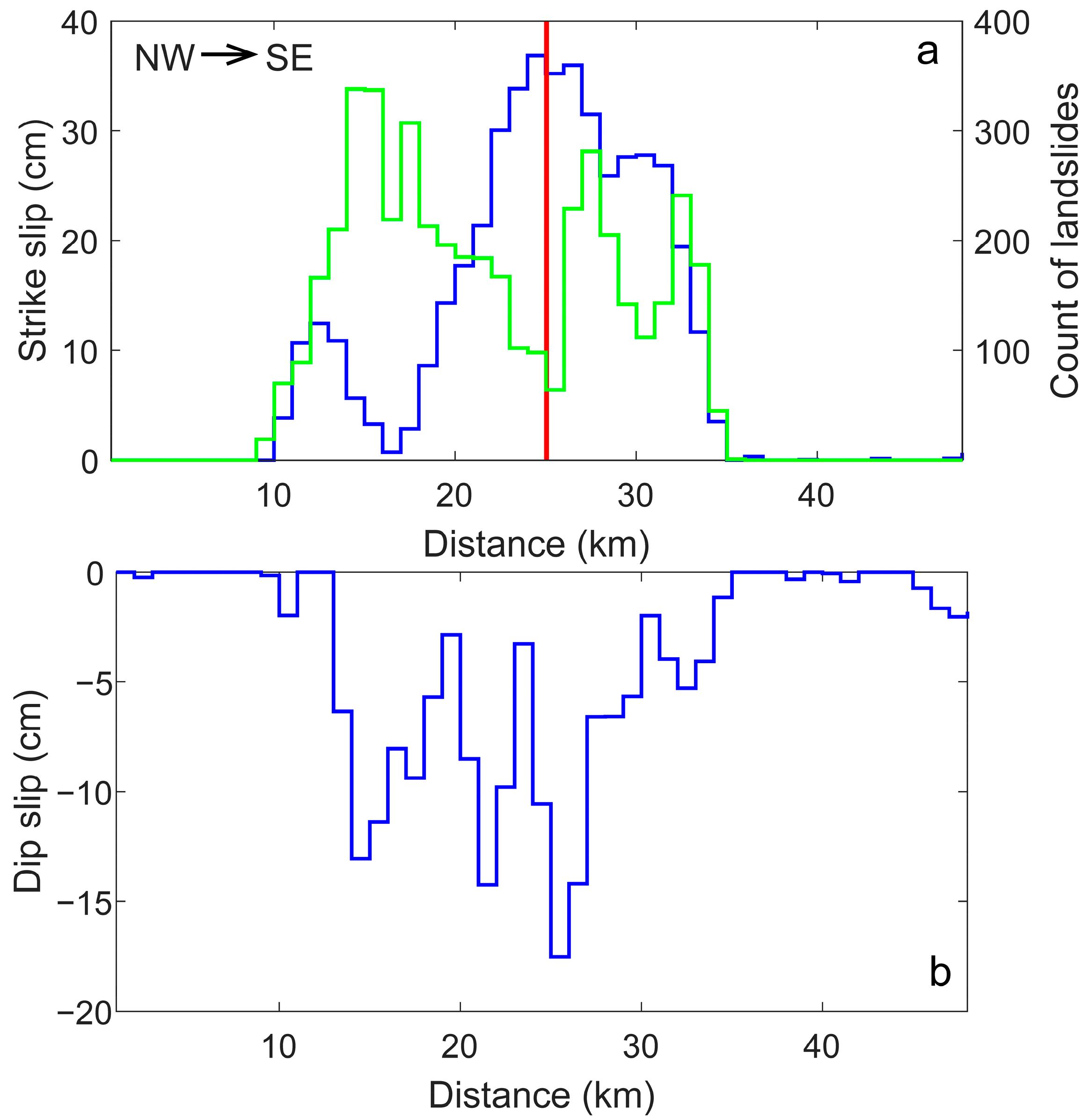
  • For a strike-slip event, the overall incidence and severity of the co-seismic landslides show a contrary distribution to the scale of the displacement of the surface rupture.

Author Contributions

Conceptualization, Z.S. and Y.Z.; data curation, Z.S. and Y.Z.; funding acquisition, Y.Z.; investigation, Z.S.; methodology, Z.S. and Y.Z.; software, Z.S. and Y.Z.; supervision, Y.Z.; validation, Z.S. and Y.Z.; visualization, Z.S. and Y.Z.; writing—original draft, Z.S. and Y.Z.; writing—review and editing, Z.S. and Y.Z. All authors have read and agreed to the published version of the manuscript.

Funding

This work is supported by the National Key Research and Development Program of China (2021YFC3000604), the National Natural Science Foundation of China (42130101, 42204004, 42072245) and the Fundamental Research Funds for the Central Universities (2042023kf0215).

Data Availability Statement

The original contributions presented in the study are included in the article, further inquiries can be directed to the corresponding author.

Acknowledgments

The authors thank the three anonymous reviewers for their thoughtful reviews and valuable comments that helped to improve the manuscript. The pre-seismic satellite optical images were obtained from Google Earth. GPS data were provided by the Beidou Foundation Reinforcement System (BFRS) and the Phase II project of the Crustal Movement Observation Network of China (CMONOC). The Sentinel-1 images are provided by the European Space Agency and freely available through the Copernicus Open Access Hub (https://scihub.copernicus.eu, accessed on 1 June 2024). The Global Centroid-Moment-Tensor (CMT) Project is available at www.globalcmt.org (accessed on 30 April 2024).

Conflicts of Interest

The authors declare no conflicts of interest.

References

  1. Han, L.; Cheng, J.; An, Y.; Fang, L.; Jiang, C.; Chen, B.; Wang, Y. Preliminary Report on the 8 August 2017 Ms 7.0 Jiuzhaigou, Sichuan, China, Earthquake. Seismol. Res. Lett. 2018, 89, 557–569. [Google Scholar] [CrossRef]
  2. Tapponnier, P.; Molnar, P. Active faulting and tectonics in China. J. Geophys. Res. Solid Earth 1977, 82, 2905–2930. [Google Scholar] [CrossRef]
  3. Teng, C.; Chang, Y.; Hsu, K.; Fan, F. On the tectonic stress field in China and its relation to plate movement. Phys. Earth Planet. Inter. 1979, 18, 257–273. [Google Scholar] [CrossRef]
  4. Xu, X.; Yu, G.; Klinger, Y.; Tapponnier, P.; Van Der Woerd, J. Reevaluation of surface rupture parameters and faulting segmentation of the 2001 Kunlunshan earthquake (Mw 7.8), northern Tibetan Plateau, China. J. Geophys. Res. Solid Earth 2006, 111, B05316. [Google Scholar] [CrossRef]
  5. Harkins, N.; Kirby, E.; Shi, X.; Wang, E.; Burbank, D.; Chun, F. Millennial slip rates along the eastern Kunlun fault: Implications for the dynamics of intracontinental deformation in Asia. Lithosphere 2010, 2, 247–266. [Google Scholar] [CrossRef]
  6. Van der Woerd, J.; Ryerson, F.J.; Tapponnier, P.; Meriaux, A.S.; Gaudemer, Y.; Meyer, B.; Finkel, R.C.; Caffee, M.W.; Zhao, G.; Xu, Z. Uniform slip-rate along the Kunlun fault: Implications for seismic behaviour and large-scale tectonics. Geophys. Res. Lett. 2000, 27, 2353–2356. [Google Scholar] [CrossRef]
  7. Van der Woerd, J.; Ryerson, F.J.; Tapponnier, P.; Meriaux, A.S.; Gaudemer, Y.; Meyer, B.; Finkel, R.C.; Caffee, M.W.; Zhao, G.; Xu, Z. Uniform postglacial slip-rate along the central 600 km of the Kunlun Fault (Tibet), from 26Al, 10Be, and 14C dating of riser offsets, and climatic origin of the regional morphology. Geophys. J. Int. 2002, 148, 356–388. [Google Scholar] [CrossRef]
  8. Kirby, E.; Whipple, K.X.; Burchfiel, B.C.; Tang, W.; Berger, G.; Sun, Z.; Chen, Z. Neotectonics of the Min Shan, China: Implications for mechanisms driving Quaternary deformation along the eastern margin of the Tibetan Plateau. Geol. Soc. Am. Bull. 2000, 112, 375–393. [Google Scholar] [CrossRef]
  9. Ren, J.; Xu, X.; Yeats, R.S.; Zhang, S. Millennial slip rates of the Tazang fault, the eastern termination of Kunlun fault: Implications for strain partitioning in eastern Tibet. Tectonophysics 2013, 608, 1180–1200. [Google Scholar] [CrossRef]
  10. Xu, C.; Wang, S.; Xu, X.; Zhang, H.; Tian, Y.; Ma, S.; Tan, X. A panorama of landslides triggered by the 8 August 2017 Jiuzhaigou, Sichuan M S 7.0 earthquake. Seismol. Geol. 2018, 40, 232–260. [Google Scholar]
  11. Liang, S.; Gan, W.; Shen, C.; Xiao, G.; Liu, J.; Chen, W.; Zhou, D. Three-dimensional velocity field of present-day crustal motion of the Tibetan Plateau derived from GPS measurements. J. Geophys. Res. Solid Earth 2013, 118, 5722–5732. [Google Scholar] [CrossRef]
  12. Deng, Q.; Zhang, P.; Ran, Y.; Yang, X.; Min, W.; Chu, Q. Basic characteristics of active tectonics of China. Sci. China Earth Sci. 2003, 46, 356–372. [Google Scholar] [CrossRef]
  13. Xie, Z.; Zheng, Y.; Yao, H.; Fang, L.; Liu, C.; Wang, M.; Shan, B.; Zhang, H.; Ren, J.; Ji, L.; et al. Preliminary analysis on the source properties and seismogenic structure of the 2017 Ms7.0 Jiuzhaigou earthquake. Sci. China Earth Sci. 2018, 61, 339–352. [Google Scholar] [CrossRef]
  14. Jones, L.; Han, W.; Hauksson, E.; Jin, A.; Zhang, Y.; Luo, Z. Focal mechanisms and aftershock locations of the Songpan earthquake of August 1976 in Sichuan, China. J. Geophys. Res. Solid Earth 1984, 89, 7697–7707. [Google Scholar] [CrossRef]
  15. Cheng, E.-L. Recent tectonic stress field and tectonic movement of the Sichuan province and its vicinity. Acta Seismol. Sin. 1981, 3, 231–241. [Google Scholar]
  16. Wells, D.; Coppersmith, K. New empirical relationships among magnitude, rupture length, rupture width, rupture area, and surface displacement. Bull Seismol. Soc. Am. 1994, 84, 974–1002. [Google Scholar] [CrossRef]
  17. Chen, W.; Qiao, X.; Liu, G.; Xiong, W.; Jia, Z.; Li, Y.; Long, F. Study on the coseismic slip model and Coulomb stress of the 2017 Jiuzhaigou Ms 7.0 earthquake constrained by GNSS and InSAR measurements. Chin. J. Geophys. 2018, 61, 2122–2132. [Google Scholar]
  18. Chen, X.; Peng, J.; Motagh, M.; Zheng, Y.; Shi, M.; Yang, H.; Jia, Q. Co-seismic deformation of the 2017 Ms 7.0 Jiuzhaigou Earthquake observed with GaoFen-3 interferometry. Int. J. Remote Sens. 2020, 41, 6618–6634. [Google Scholar] [CrossRef]
  19. Hong, S.; Zhou, X.; Zhang, K.; Meng, G.; Dong, Y.; Su, X.; Zhang, L.; Li, S.; Ding, K. Source model and stress disturbance of the 2017 Jiuzhaigou Mw 6.5 earthquake constrained by InSAR and GPS measurements. Remote Sens. 2018, 10, 1400. [Google Scholar] [CrossRef]
  20. Ji, L.; Liu, C.; Xu, J.; Liu, L.; Long, F.; Zhang, Z. InSAR observation and inversion of the seismogenic fault for the 2017 Jiuzhaigou MS 7.0 earthquake in China. Chin. J. Geophys. 2017, 60, 4069–4082. [Google Scholar]
  21. Li, Y.; Bürgmann, R.; Zhao, B. Evidence of fault immaturity from shallow slip deficit and lack of postseismic deformation of the 2017 Mw 6.5 Jiuzhaigou earthquake. Bull. Seism. Soc. Am. 2020, 110, 154–165. [Google Scholar] [CrossRef]
  22. Liu, G.; Xiong, W.; Wang, Q.; Qiao, X.; Ding, K.; Li, X.; Yang, S. Source characteristics of the 2017 Ms 7.0 Jiuzhaigou, China, earthquake and implications for recent seismicity in eastern Tibet. J. Geophys. Res. Solid Earth 2019, 124, 4895–4915. [Google Scholar] [CrossRef]
  23. Nie, Z.; Wang, D.; Jia, Z.; Yu, P.; Li, L. Fault model of the 2017 Jiuzhaigou Mw 6.5 earthquake estimated from coseismic deformation observed using Global Positioning System and Interferometric Synthetic Aperture Radar data. Earth Planets Space 2018, 70, 55. [Google Scholar] [CrossRef]
  24. Peng, W.; Huang, X.; Wang, Z. Coseismic deformation and fault inversion of the 2017 Jiuzhaigou Ms 7.0 Earthquake: Constraints from steerable pyramid and InSAR observations. Remote Sens. 2022, 15, 222. [Google Scholar] [CrossRef]
  25. Shan, X.; Qu, C.; Gong, W.; Zhao, D.; Zhang, G. Coseismic deformation field of the Jiuzhaigou Ms 7.0 earthquake from Sentinel-1A InSAR data and fault slip inversion. Chin. J. Geophys. 2017, 60, 4527–4536. [Google Scholar]
  26. Shen, W.; Li, Y.S.; Jiao, Q.; Xie, Q.; Zhang, J. Joint inversion of strong motion and InSAR/GPS data for fault slip distribution of the Jiuzhaigou 7.0 earthquake and its application in seismology. Chin. J. Geophys. 2019, 61, 115–129. [Google Scholar]
  27. Sun, J.; Yue, H.; Shen, Z.; Fang, L.; Zhan, Y.; Sun, X. The 2017 Jiuzhaigou earthquake: A complicated event occurred in a young fault system. Geophys. Res. Lett. 2018, 45, 2230–2240. [Google Scholar] [CrossRef]
  28. Tang, X.; Guo, R.; Xu, J.; Sun, H.; Chen, X.; Zhou, J. Probing the fault complexity of the 2017 Ms 7.0 Jiuzhaigou earthquake based on the InSAR data. Remote Sens. 2021, 13, 1573. [Google Scholar] [CrossRef]
  29. Wang, J.; Shan, X.; Zhang, G. Fault slip distribution inversion and co-seismic deformation of the 2017 Jiuzhaigou Ms 7.0 earthquake based on InSAR. North China Earthq. Sci. 2018, 36, 1–7. [Google Scholar]
  30. Zhang, X.; Feng, W.P.; Xu, L.S.; Li, C.L. The source-process inversion and the intensity estimation of the 2017 Ms 7.0 Jiuzhaigou earthquake. Chin. J. Geophys. 2017, 60, 4105–4116. [Google Scholar]
  31. Zhang, Y.; Zhang, G.; Hetland, E.; Shan, X.; Zhang, H.; Zhao, D.; Gong, W.; Qu, C. Source fault and slip distribution of the 2017 Mw 6.5 Jiuzhaigou, China, earthquake and its tectonic implications. Seismol. Res. Lett. 2018, 89, 1345–1353. [Google Scholar] [CrossRef]
  32. Zhang, X.; Xu, L.; Yi, L.; Feng, W. Confirmation and characterization of the rupture model of the 2017 Ms 7.0 Jiuzhaigou, China, earthquake. Seismol. Res. Lett. 2021, 92, 2927–2942. [Google Scholar] [CrossRef]
  33. Zhang, Y.; Feng, W.; Li, X.; Liu, Y.; Ning, J.; Huang, Q. Joint inversion of rupture across a fault stepover during the 8 August 2017 Mw 6.5 Jiuzhaigou, China, earthquake. Seismol. Res. Lett. 2021, 92, 3386–3397. [Google Scholar] [CrossRef]
  34. Zhao, D.; Qu, C.; Shan, X.; Gong, W.; Zhang, Y.; Zhang, G. InSAR and GPS derived coseismic deformation and fault model of the 2017 Ms 7.0 Jiuzhaigou earthquake in the Northeast Bayanhar block. Tectonophysics 2018, 726, 86–99. [Google Scholar] [CrossRef]
  35. Zheng, A.; Yu, X.; Xu, W.; Chen, X.; Zhang, W. A hybrid source mechanism of the 2017 Mw 6.5 Jiuzhaigou earthquake revealed by the joint inversion of strong-motion, teleseismic and InSAR data. Tectonophysics 2020, 789, 228538. [Google Scholar] [CrossRef]
  36. Ding, K.; He, P.; Wen, Y.; Chen, Y.; Wang, D.; Li, S.; Wang, Q. The 2017 Mw 7.3 Ezgeleh, Iran earthquake determined from InSAR measurements and teleseismic waveforms. Geophys. J. Int. 2018, 215, 1728–1738. [Google Scholar] [CrossRef]
  37. Hanssen, R.F. Radar Interferometry: Data Interpretation and Error Analysis; Kluwer Academic Publishers: Dordrecht, The Netherlands, 2001. [Google Scholar]
  38. Herring, T.; King, R.W.; McClusky, S.C. Introduction to Gamit/Globk; Massachusetts Institute of Technology: Cambridge, MA, USA, 2010. [Google Scholar]
  39. Rosen, P.A.; Gurrola, E.; Sacco, G.F.; Zebker, H. The InSAR scientific computing environment. In Proceedings of the EUSAR 2012 9th European Conference on Synthetic Aperture Radar, Nuremberg, Germany, 23–26 April 2012. [Google Scholar]
  40. Chen, C.W.; Zebker, H.A. Phase unwrapping for large SAR interferograms: Statistical segmentation and generalized network models. IEEE Trans. Geosci. Remote Sens. 2002, 40, 1709–1719. [Google Scholar] [CrossRef]
  41. Welstead, S.T. Fractal and Wavelet Image Compression Techniques; SPIE Press: Bellingham, WA, USA, 1999; Volume 40. [Google Scholar]
  42. Jónsson, S.; Zebker, H.; Segall, P.; Amelung, F. Fault slip distribution of the 1999 Mw 7.1 Hector Mine, California, earthquake, estimated from satellite radar and GPS measurements. Bull. Seismol. Soc. Am. 2002, 92, 1377–1389. [Google Scholar] [CrossRef]
  43. Jiang, G.; Xu, C.; Wen, Y.; Liu, Y.; Yin, Z.; Wang, J. Inversion for coseismic slip distribution of the 2010 Mw 6.9 Yushu earthquake from InSAR data using angular dislocations. Geophys. J. Int. 2013, 194, 1011–1022. [Google Scholar] [CrossRef]
  44. Okada, Y. Internal deformation due to shear and tensile faults in a half-space. Bull. Seismol. Soc. Am. 1992, 82, 1018–1040. [Google Scholar] [CrossRef]
  45. Stark, P.B.; Parker, R.L. Bounded variable least squares: An algorithm and application. J. Comput. Stat. 1995, 10, 129–141. [Google Scholar]
  46. Lohman, R.B.; Simons, M. Some thoughts on the use of InSAR data to constrain models of surface deformation: Noise structure and data downsampling, Geochem. Geophys. Geosyst. 2005, 6, Q01007. [Google Scholar] [CrossRef]
  47. Chen, S.F.; Wilson, C.J.L.; Deng, Q.D.; Zhao, X.L. Active faulting and block movement associated with large earthquakes in the Min Shan and Longmen Mountains, northeastern Tibetan Plateau. J. Geophys. Res. Solid Earth 1994, 99, 24025–24038. [Google Scholar] [CrossRef]
  48. Li, Y.; Zhou, R.; Densmore, A.L.; Ellis, M.A. The Geology of the Eastern Margin of the Qinghai-Tibet Plateau; Geological Publishing House: Beijing, China, 2006. (In Chinese) [Google Scholar]
  49. Zhao, X.; Deng, Q.; Chen, S. Tectonic geomorphology of the Minshan uplift in western Sichuan, southwestern China. Seismol. Geol. 1994, 16, 429–439. (In Chinese) [Google Scholar]
  50. Zhao, B.; Su, L.; Qiu, C.; Lu, H.; Zhang, B.; Zhang, J.; Geng, X.; Chen, H.; Wang, Y. Understanding of landslides induced by 2022 Luding earthquake, China. J. Rock Mech. Geotech. 2024. [Google Scholar] [CrossRef]
  51. Dai, L.; Xu, Q.; Fan, X.; Chang, M.; Yang, Q.; Yang, F.; Ren, J. A preliminary study on spatial distribution patterns of landslides triggered by Jiuzhaigou earthquake in Sichuan on August 8th, 2017 and their susceptibility assessment. J. Eng. Geol. 2017, 25, 1151–1164. (In Chinese) [Google Scholar]
  52. Fan, X.; Scaringi, G.; Xu, Q.; Zhan, W.; Dai, L.; Li, Y.; Pei, X.; Yang, Q.; Huang, R. Coseismic landslides triggered by the 8th August 2017 Ms 7.0 Jiuzhaigou earthquake (Sichuan, China): Factors controlling their spatial distribution and implications for the seismogenic blind fault identification. Landslides 2018, 15, 967–983. [Google Scholar] [CrossRef]
  53. Tian, Y.; Xu, C.; Ma, S.; Xu, X.; Wang, S.; Zhang, H. Inventory and spatial distribution of landslides triggered by the 8th August 2017 MW 6.5 Jiuzhaigou earthquake, China. J. Earth Sci. 2019, 30, 206–217. [Google Scholar] [CrossRef]
Figure 1. Tectonic setting of the 8 August 2017 Jiuzhaigou earthquake. Black arrows with error ellipses of 95% confidence are the interseismic GPS velocities [11]. Red lines are the major faults in the seismic region from a map of active tectonics in China [12]. ATF: Altyn Tagh Fault, KLF: Kunlun Fault, XSHF: Xianshuihe Fault, JLF: Jiali Fault, RRF: Red River Fault, TZF: Tazang Fault, WXF: Wenxian Fault, HYF: Huya Fault, MJF: Minjiang Fault. Green circles are the relocated aftershocks up to 21 August [13]. Yellow lines are the surface trace of the rupture fault extracted from pre-seismic satellite images. Blue stars mark the hypocenters of historical earthquakes. The red star shows the hypocenter of the 2017 Jiuzhaigou earthquake. The focal mechanisms of the triplet of earthquakes in 1976 and the 1973 Ms 6.5 earthquake are from Jones et al. [14] and Cheng [15], respectively. The focal mechanisms of the other earthquakes were retrieved from GCMT. The two black rectangles outline the coverage of the ascending and descending Sentinel-1 InSAR data. The purple dashed rectangle was used to clip the InSAR interferograms for subsequent inversions.
Remotesensing 16 03406 g001
Figure 2. Fault traces of the 2017 Jiuzhaigou earthquake fault. (a) Active tectonics around the epicenter (red star) of the Jiuzhaigou earthquake. Yellow lines are the surface trace of the rupture fault extracted from pre-seismic satellite images. The Red line is the simplified seismogenic fault for joint inversions of GPS and InSAR data. Green spots mark the co-seismic landslides. Blue rectangles outline the areas shown in panels (bd). (b) Offset features northwest of Xiongmao Lake, including beheaded and deflected channels, displaced ridges and a linear fault trough. Relative motions along the fault are indicated with red arrows. (c) Displaced ridges and sag pond southeast of Xiongmao Lake. (d) Displaced ridges and fault valley near Shawu Village.
Remotesensing 16 03406 g002
Figure 3. GPS and InSAR observations used in this study. Panels (a,b) are the co-seismic ascending and descending interferometric fringe patterns. Panels (c,d) are the prediction results. Panels (e,f) are the residual interferometric fringes. The black lines are the surface trace of the northern Huya Fault extracted from pre-seismic optical images. The red line is the simplified seismogenic fault for joint inversions of GPS and InSAR data. Observed and predicted GPS horizontal displacements are plotted with black and red arrows, respectively. The black rectangle in Panel (c) outlines the area shown in Figure 6a.
Remotesensing 16 03406 g003
Figure 4. The finite fault slip models of the Jiuzhaigou earthquake derived from joint inversions of GPS and InSAR observations. Panel (a) shows variable GPS misfit with increasing weight ratios between GPS and InSAR data. Panel (b) shows variable GPS misfit with increasing fault dip angles. Panel (c) shows the trade-off curves between the model residuals and the roughness of slip models. Panel (d) shows the resulting slip model. Red stars mark the selected values.
Remotesensing 16 03406 g004
Figure 5. Swath profiles across the northern, middle and southern segments of the Huya Fault. (a) Active tectonics around the Huya fault. Yellow lines are the surface trace of the rupture fault extracted from pre-seismic satellite images. The Red line is the simplified seismogenic fault for joint inversions of GPS and InSAR data. Red stars show the epicenters of the historical earthquakes since 1973 along the Huya Fault. Black rectangles outline the areas of Swath profiles show in panels (bd). In panels (bd), topography within ~10 km from the profile is plotted: average topography is plotted with a black curve, and maximum and minimum topography are plotted with gray curves. The crosses/dots and red arrow indicate the in–out fault motion directions and reversing direction. Red lines in the three profiles indicate the site of the Huya Fault.
Remotesensing 16 03406 g005
Figure 6. (a) A close-up view of landslides and the ascending P128A LOS displacement map. (b) Statistical results of the largest LOS displacement in each landslide region.
Remotesensing 16 03406 g006
Figure 7. Potential surface rupture magnitudes of the Jiuzhaigou earthquake derived from the slip model in Figure 4a. The blue lines in panels (a,b) are the strike- and dip-slip components, respectively. The green line denotes the number of landslides along the fault strike. The red line marks the fault center.
Remotesensing 16 03406 g007
Table 1. Focal parameters of the Jiuzhaigou earthquake.
SourceStrike (°)Dip (°)Rake (°) *Patch Size (km)Max Slip (m)Depth (km) †Seismic Moment (N m)DataMisfit
USGS15384−33 7.228 × 10¹⁸
GCMT15078−13 7.62 × 10¹⁸
Chen et al. [17]15581−9.562 × 20.9110.867.754 × 1018Sentinel-1A P128A and P062D; 2 GPS sites
Chen et al. [18]15580~01 × 1~110–13 GaoFen-3 ascending path
Hong et al. [19]154.2177.0−7.861 × 11.066.847.85 × 1018Sentinel-1A P128A and P062D; RADARSAT-2 ascending path; 10 GPS sites1.9 cm; 1.4 cm; 0.8 cm; 0.2 cm
Ji et al. [20] 61–90~02 × 20.89.0 Sentinel-1A P128A, P055A and P062D
Li et al. [21]15870 1.23–10 Sentinel-1A P128A and P062D; 4 GPS sites1.028 cm; 0.262 cm
Liu et al. [22]148–17188 2 × 2 9.0 × 10¹⁸Sentinel-1A P128A and P062D; 10 GPS sites; high-rate GPS and teleseismic waveforms~3 cm
Nie et al. [23]15581−112 × 20.8511.06.6 × 1018Sentinel-1A P128A and P062D; 8 GPS sites0.25 cm; ~0.2 cm
Peng et al. [24]15050 2 × 20.7793.98 × 1018Sentinel-1A P128A and P062D
Shan et al. [25]15350~−9 ‡2 × 2~1~8 Sentinel-1A P128A and P062D
Shen et al. [26]153 2 × 20.74 7.6 × 10¹⁸Sentinel-1A P128A and P062D; 7 GPS sites; 8 strong-motion sites2.55 cm
Sun et al. [27]1518554.8~2 × 22.69.07.6 × 1018Sentinel-1A P128A and P062D; teleseismic waveforms
Tang et al. [28]151–19677 2 × 21.51 6.3 × 10¹⁸Sentinel-1A P128A
Wang et al. [29]15482−22 ‡2 × 10.687.59.6 × 1018Sentinel-1A P128A and P062D1.2 cm; 0.7 cm
Zhang et al. [30]15384−142 × 21.0 6.61 × 10¹⁸Sentinel-1A P128A; teleseismic waveforms1.93 cm; 0.81
Zhang et al. [31]15350−122 × 2~166.3 × 10¹⁸Sentinel-1A P128A and P062D; 2 GPS sites1.4 cm
Zhang et al. [32]15679 2 × 21.86.46.6 × 1018Sentinel-1A P128A and P062D; teleseismic waveforms; near-field seismic and strong-motion waveforms
Zhang et al. [33]130–15157–70 2 × 2 5.2 × 10¹⁸Sentinel-1A P128A and P062D; high-rate GPS and teleseismic and strong-motion waveforms
Zhao et al. [34]11580−101 × 11.36.06.8 × 1018Sentinel-1A P128A and P062D; 2 GPS sites~6 cm
Zheng et al. [35]145–151.483.6 2 × 20.8 7.9 × 10¹⁸Sentinel-1A P128A and P062D; teleseismic and strong-motion waveforms
This study15377 1 × 11.126.85.3 × 1018Sentinel-1A P128A and P062D; 7 GPS sites1.5 cm; 1.6 cm; 0.1 cm
* The rake angle of the maximum slip. ‡ The average rake angle. † The depth of the maximum slip.
Table 2. Horizontal co-seismic displacements at seven GPS sites.
SiteLocationDisplacement (mm)Error (mm)
LongitudeLatitudeENEN
BDWD104.91°E33.40°N−2.50.91.31.2
GSWD104.82°E33.42°N−0.81.30.60.9
GSWX104.68°E32.95°N−2.60.91.10.8
GSZQ104.25°E33.80°N0.43.61.20.8
SCJZ104.25°E33.24°N−9.83.31.50.7
SCPW104.54°E32.41°N−0.41.31.41.1
SCSP103.58°E32.65°N−1.8−7.70.70.6
Table 3. Details of two Sentinel-1 InSAR interferograms.
IDOrbitMasterSlavePerpendicular Baseline
YYYY/MM/DDYYYY/MM/DD(m)
P128AAscending2017/07/302017/08/11−37
P062DDescending2017/08/062017/08/1867
Disclaimer/Publisher’s Note: The statements, opinions and data contained in all publications are solely those of the individual author(s) and contributor(s) and not of MDPI and/or the editor(s). MDPI and/or the editor(s) disclaim responsibility for any injury to people or property resulting from any ideas, methods, instructions or products referred to in the content.

