Article

Development of a UAS-Based Multi-Sensor Deep Learning Model for Predicting Napa Cabbage Fresh Weight and Determining Optimal Harvest Time

1
Geospatially Enabled Society Research Center, Korea Research Institute for Human Settlements, 5 Gukchaegyeonguwon-ro, Sejong 30147, Republic of Korea
2
Department of Agricultural and Rural Engineering, Chungbuk National University, 1 Chungdae-ro, Seowon-gu, Cheongju 28644, Republic of Korea
*
Author to whom correspondence should be addressed.
Remote Sens. 2024, 16(18), 3455; https://doi.org/10.3390/rs16183455
Submission received: 13 July 2024 / Revised: 1 September 2024 / Accepted: 9 September 2024 / Published: 18 September 2024

Abstract

:
The accurate and timely prediction of Napa cabbage fresh weight is essential for optimizing harvest timing, crop management, and supply chain logistics, which ultimately contributes to food security and price stabilization. Traditional manual sampling methods are labor-intensive and lack precision. This study introduces an artificial intelligence (AI)-powered model that utilizes unmanned aerial systems (UAS)-based multi-sensor data to predict Napa cabbage fresh weight. The model was developed using high-resolution RGB, multispectral (MSP), and thermal infrared (TIR) imagery collected throughout the 2020 growing season. The imagery was used to extract various vegetation indices, crop features (vegetation fraction, crop height model), and a water stress indicator (CWSI). The deep neural network (DNN) model consistently outperformed support vector machine (SVM) and random forest (RF) models, achieving the highest accuracy (R2 = 0.82, RMSE = 0.47 kg) during the mid-to-late rosette growth stage (35–42 days after planting, DAP). The model’s accuracy improved with cabbage maturity, emphasizing the importance of the heading stage for fresh weight estimation. The model slightly underestimated the weight of Napa cabbages exceeding 5 kg, potentially due to limited samples and saturation effects of vegetation indices. The overall error rate was less than 5%, demonstrating the feasibility of this approach. Spatial analysis further revealed that the model accurately captured variability in Napa cabbage growth across different soil types and irrigation conditions, particularly reflecting the positive impact of drip irrigation. This study highlights the potential of UAS-based multi-sensor data and AI for accurate and non-invasive prediction of Napa cabbage fresh weight, providing a valuable tool for optimizing harvest timing and crop management. Future research should focus on refining the model for specific weight ranges and diverse environmental conditions, and extending its application to other crops.

Graphical Abstract

1. Introduction

1.1. The Growing Demand for Precision Agriculture

In the face of a burgeoning global population and the escalating pressures of climate change, ensuring food security and maximizing agricultural productivity have become paramount concerns [1,2,3]. To achieve these goals, farmers and agricultural stakeholders are increasingly turning to precision agriculture, a data-driven approach that optimizes crop management practices based on real-time information and analysis. Accurate prediction of crop yield is a fundamental aspect of precision agriculture, as it enables informed decision-making regarding resource allocation, harvest timing, and supply chain management [4,5].

1.2. The Importance of Accurate Napa Cabbage Fresh Weight Prediction in Modern Agriculture

Napa cabbage (Brassica rapa L. ssp. pekinensis), a staple crop in East Asia, plays a vital role in regional diets and economies. However, its production faces numerous challenges, including susceptibility to price fluctuations due to its short storage life and sensitivity to environmental factors such as abnormal weather patterns and fluctuating cultivation areas [6,7,8]. Accurate and timely prediction of Napa cabbage yield is crucial for efficient resource allocation, effective supply chain management, and price stabilization. The accurate prediction of Napa cabbage fresh weight is crucial for mitigating these challenges and ensuring a stable supply of this essential crop.
The ability to accurately predict Napa cabbage fresh weight before harvest offers numerous benefits to various stakeholders in the agricultural sector. Farmers: Precise yield prediction empowers farmers to make informed decisions regarding harvest timing, ensuring optimal quality, and maximizing market value while minimizing post-harvest losses [9,10]. Additionally, it enables farmers to tailor crop management strategies, such as irrigation and fertilization, based on real-time insights into crop growth and development, thereby improving resource use efficiency and reducing environmental impact [11,12,13]. Agribusinesses: Reliable yield forecasts facilitate better supply chain management, ensuring adequate inventory levels, reducing food waste, and mitigating price volatility [14]. This leads to increased profitability and a more stable market for both producers and consumers. Policymakers: Accurate yield predictions inform national-level decision-making, enabling governments to develop effective agricultural policies, anticipate potential shortages, and implement measures to ensure food security [15,16]. This is particularly crucial in the context of climate change, where unpredictable weather patterns can significantly impact crop yields.

1.3. Limitations of Traditional Methods and the Rise of UAS-Based Remote Sensing

Traditional methods for estimating Napa cabbage fresh weight, such as manual sampling and visual inspection, are labor-intensive, time-consuming, and prone to human error [17]. These methods also lack the spatial and temporal resolution necessary for precise field-scale assessment, making it difficult to detect subtle variations in crop growth. While satellite imagery offers a broader perspective, it may not capture the nuanced variations in Napa cabbage growth and development at the field level [18,19].
The integration of unmanned aerial systems (UAS) with advanced sensors and artificial intelligence (AI) algorithms presents a transformative solution to these limitations. UAS, or drones, equipped with high-resolution RGB, multispectral (MSP), thermal infrared (TIR) sensors, and hyperspectral sensors, can efficiently collect detailed data on crop health, vigor, and yield potential at a fine spatial and temporal scale [20,21,22,23,24,25]. These data, coupled with the computational power of AI, enable the development of sophisticated models for predicting crop yield and other essential parameters.

1.4. The Power of AI in Agriculture

The fusion of AI algorithms with UAS-based remote sensing data has significantly enhanced the capabilities of yield prediction models. Numerous studies have demonstrated the potential of UAS-based remote sensing and AI in various agricultural applications, including crop classification [26,27], growth monitoring [28], nutritional status assessment [29,30], yield prediction [31,32,33], and disease detection [34,35]. AI algorithms, particularly deep learning techniques, excel at processing large volumes of data and identifying complex patterns and relationships that may not be apparent through traditional statistical methods. They have shown exceptional promise in extracting meaningful features from UAS imagery and accurately predicting crop yield, even in complex and dynamic environments [36].

1.5. Objectives and Contributions

This study aims to address the current limitations in Napa cabbage fresh weight prediction by developing a comprehensive AI-powered model that leverages UAS-based multi-sensor data. Specifically, this study aims to: (1) Develop a robust and accurate model for predicting Napa cabbage fresh weight by integrating RGB, MSP, and TIR imagery with AI algorithms, including deep neural networks (DNN), support vector machines (SVM), and random forests (RF). (2) Identify the optimal growth stage during the Napa cabbage growth cycle for achieving the most accurate fresh weight predictions. (3) Evaluate the performance of the developed models using various evaluation metrics, focusing on accuracy, generalizability, and robustness. (4) Analyze the spatial variability of Napa cabbage fresh weight and its prediction, investigating the influence of soil type and irrigation practices. (5) Discuss the limitations of the current approach and propose potential avenues for future research to further enhance the accuracy and applicability of fresh weight prediction models.
By achieving these objectives, this study contributes to the advancement of precision agriculture for Napa cabbage cultivation, offering a valuable tool for optimizing harvest timing, improving crop management practices, and enhancing supply chain efficiency.

2. Materials and Methods

2.1. Study Area and Experimental Plot Design

This study was conducted in 2020 at the Napa cabbage cultivation test field of the National Institute of Agricultural Sciences, located in Iseo-myeon, Wanju-gun, Jeollabuk-do, Republic of Korea (127°02′49.65″E, 35°49′28.52″N) (Figure 1). The experimental plots were designed on a slope of approximately 7 degrees to simulate the typical terrain of Napa cabbage cultivation areas in Korea.
The test field comprised three plots, each with an area of 290 m2, and distinct soil conditions: clay loam, loam, and sandy loam. Each plot measured 25.5 m × 11.7 m. The study focused on fall Napa cabbage (‘Cheongomabi’ variety), planted in late August and harvested in early November, with a planting distance of 0.45 m × 0.85 m. Standard cultivation methods were employed throughout the study period.
In 2020, a non-watering treatment was implemented for the Napa cabbage grown in the loam plot, relying solely on rainfall for water supply. The other two plots (clay loam and sandy loam) were maintained under standard irrigation practices.

2.2. Unmanned Aerial System (UAS) and Sensors

A rotary-wing UAS, the Inspire 2 (DJI, Shenzhen, China), was utilized for image acquisition throughout the fall Napa cabbage growth cycle. The UAS was equipped with three distinct sensors: A Zenmuse X5S (DJI, Shenzhen, China) RGB camera with a 20-megapixel resolution to capture standard red, green, and blue (RGB) light wavelengths. A RedEdge-M (MicaSense, Seattle, WA, USA) MSP sensor designed to capture light wavelengths beyond the visible spectrum, providing valuable insights into plant health and vegetation indices. A Vue Pro R (FLIR, Wilsonville, OR, USA) TIR sensor capable of measuring the thermal radiation emitted by objects, enabling the assessment of plant temperature and water stress.
This integrated multi-sensor approach facilitated the collection of comprehensive data encompassing Napa cabbage’s morphological, physiological, and thermal characteristics throughout the growing season. Image acquisition was conducted with a 75% overlap in both longitudinal and lateral directions to ensure adequate coverage and enable accurate image stitching. The RGB imagery was collected in a double-grid pattern for improved 3D information extraction, while the MSP and TIR imagery followed a standard grid pattern. Flight altitude was maintained at 30 m above ground level to achieve the desired spatial resolution.

2.3. Fall Napa Cabbage Growth Cycle and Data Collection Timeline

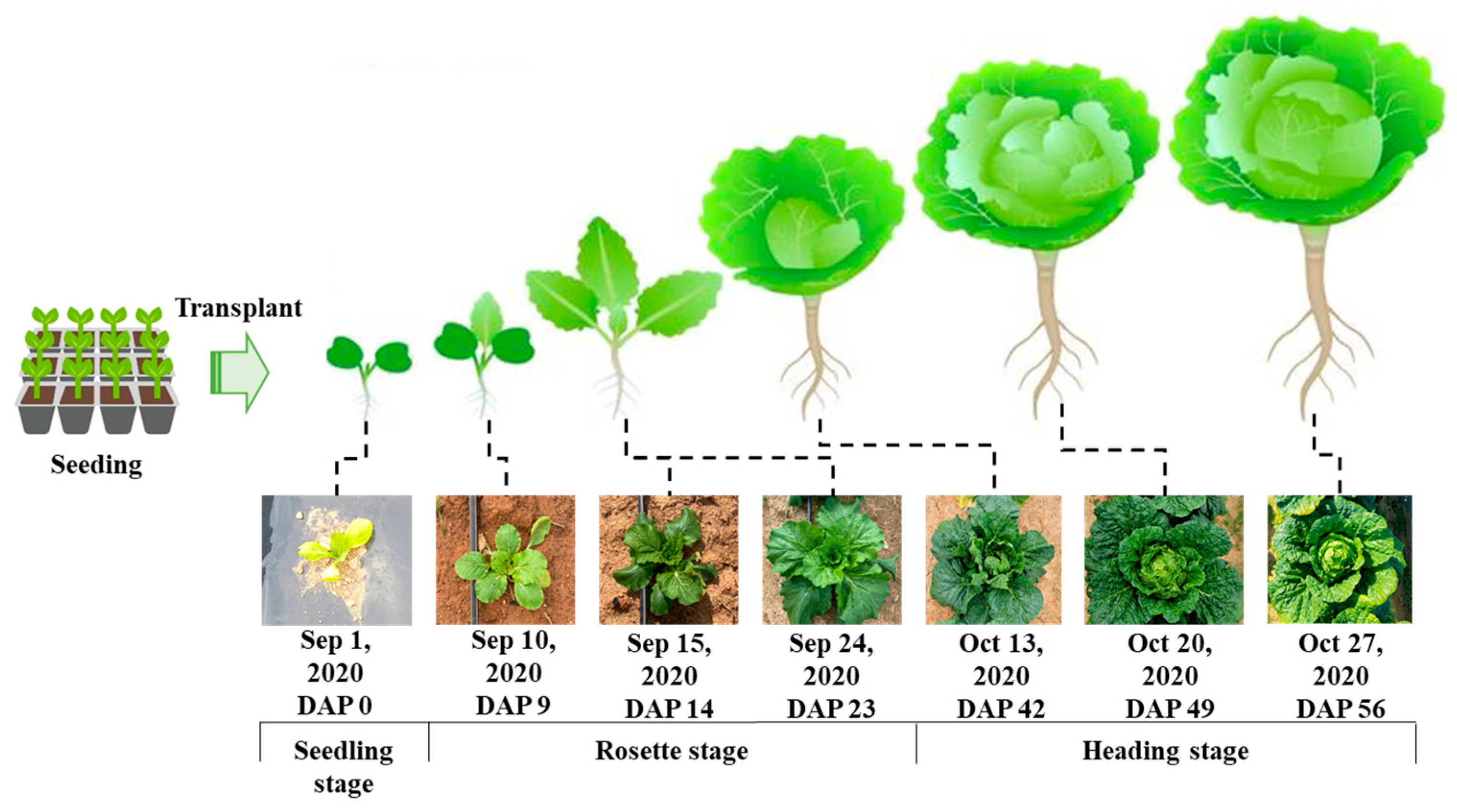
Fall Napa cabbage (cv. ‘Cheongomabi’) typically follows a 70-day growth cycle, starting from late August planting to early November harvest. In this study, seedlings were sown in pots and transplanted to the field after 15–20 days. The growth cycle is characterized by three distinct stages (Figure 2): The Seedling Stage (days after planting, DAP 0–7), which is the initial that encompasses root establishment and early vegetative growth post-transplanting. The Rosette Stage (DAP 9–42), which is the longest growth phase and marked by a rapid increase in leaf number and expansion of leaf area. The Heading Stage (DAP 49–56), the final stage, which is characterized by the cessation of leaf growth and the formation of a compact, spherical head as the inner leaves mature.
To monitor the entire growth cycle for the fresh weight prediction model, UAS imaging and field surveys were conducted at 7~10-day intervals from late August to early November, capturing data across all growth stages, including the pre-planting period, as detailed in Table 1.

2.4. Study Flow Chart

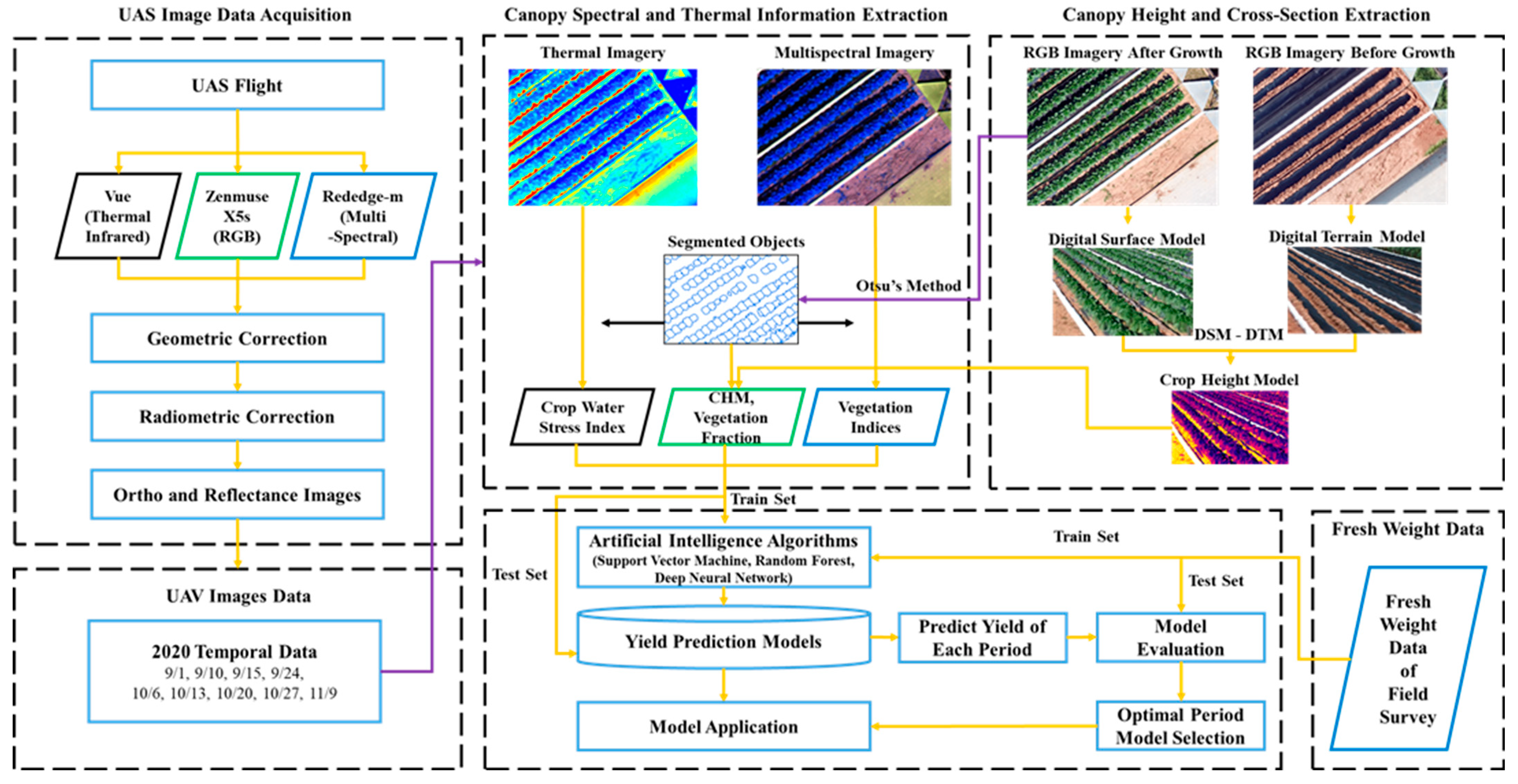
The overall study process, as depicted in Figure 3, followed a systematic sequence: data collection, image preprocessing, data preprocessing, AI model construction and evaluation, and, ultimately, fresh weight prediction for each fall Napa cabbage plant.
UAS imagery and corresponding field data were collected in 2020. The acquired images underwent preprocessing, including geometric and radiometric corrections, to ensure accuracy and consistency. Utilizing the 2020 time-series data, further preprocessing was conducted to extract relevant features and normalize the data for subsequent analysis. AI models were then constructed and evaluated for each data collection date, employing a range of algorithms to identify the optimal model for fresh weight prediction. The selection of the final model involved assessing its performance at different growth stages and determining the most effective algorithm.
The detailed methodologies for each stage of the fresh weight study, including image preprocessing, data preprocessing, AI model construction and evaluation, and fresh weight calculation, are presented in subsequent sections as outlined in Figure 3.

2.5. UAS Image Acquisition and Preprocessing

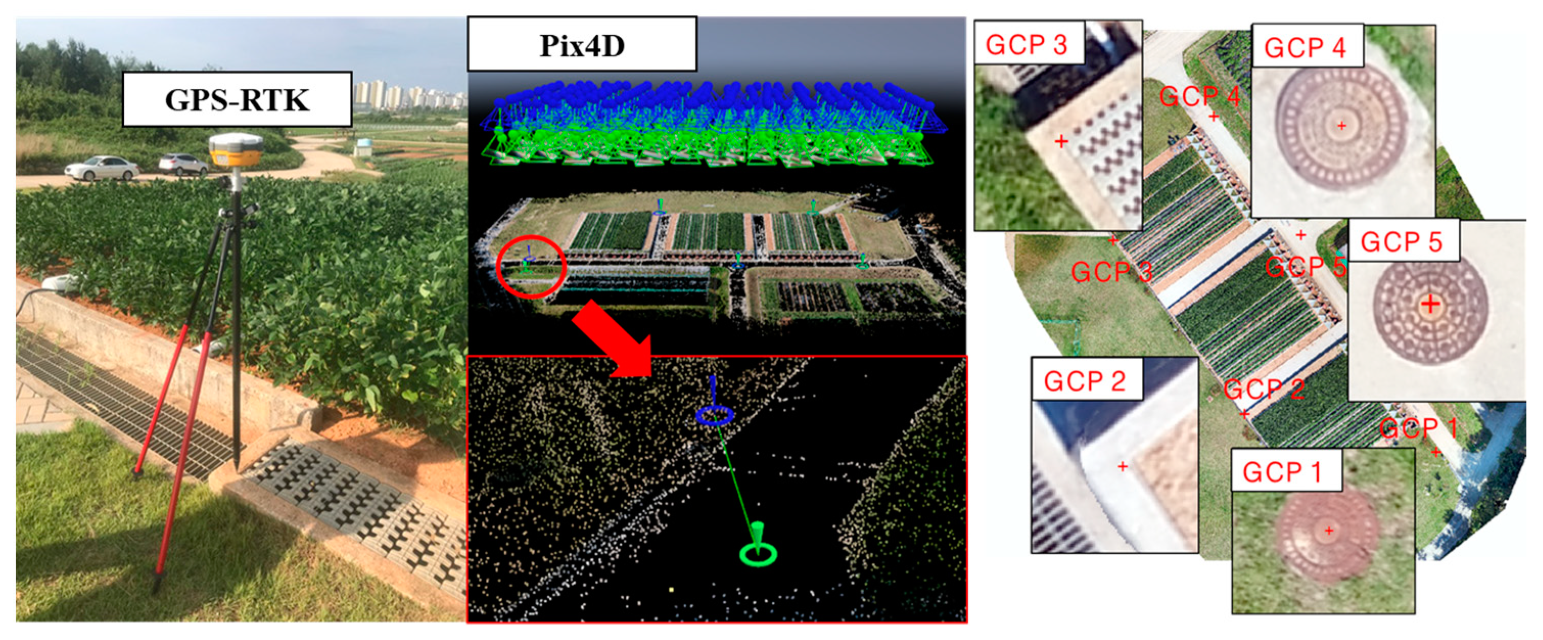
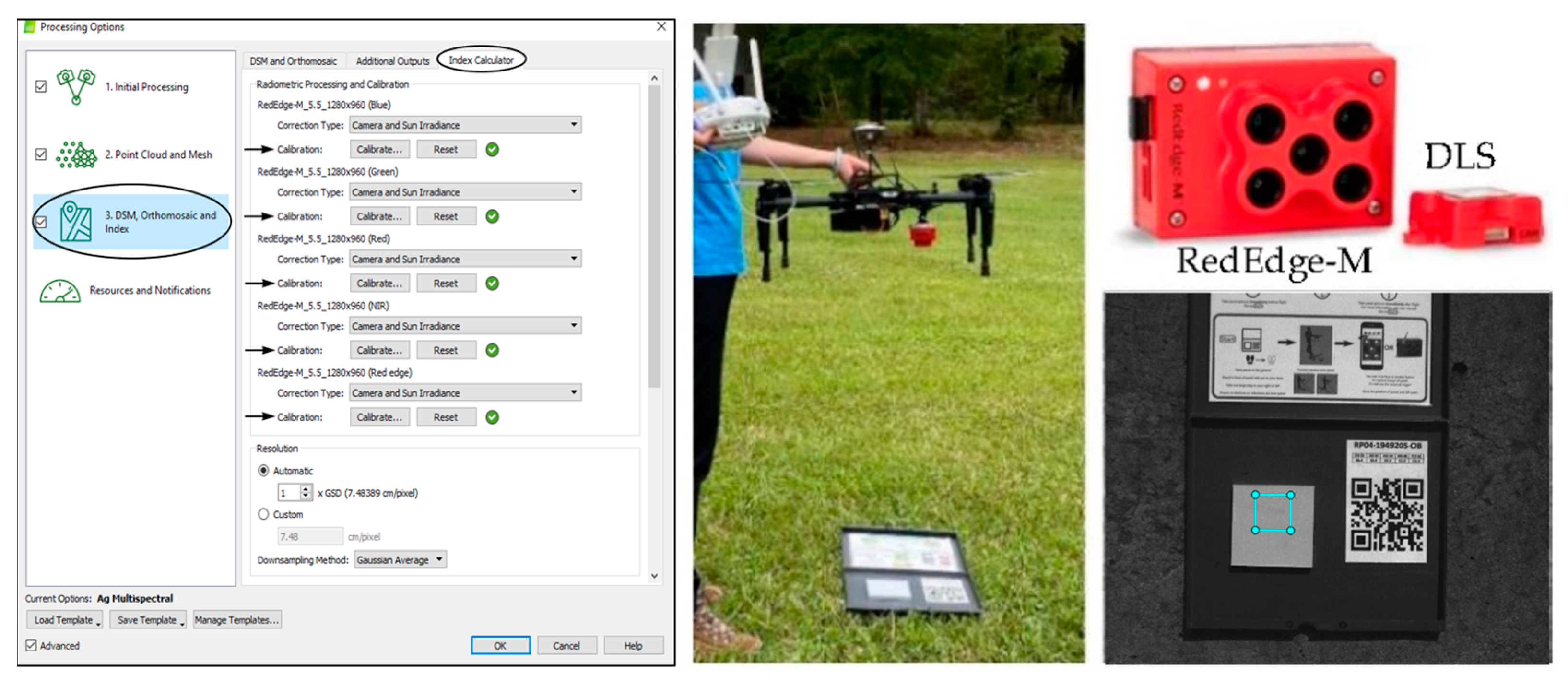
UAS imagery was captured at a 30 m altitude using a DJI Inspire 2 UAS. The imagery was captured with an overlap of 75% in both the longitudinal and lateral directions. The RGB imagery was collected in a double-grid pattern to ensure higher accuracy in 3D information, while the MSP and TIR imagery was captured using a standard grid pattern. The acquired MSP imagery underwent geometric and radiometric correction using Pix4D mapper (Pix4D, Prilly, Switzerland) software version 4.8.8. Geometric correction was achieved by incorporating the measured co-ordinates of five ground control points (GCPs), selected on unchanging objects within the field (e.g., manholes), into the preprocessing workflow (Figure 4). Radiometric correction was performed using both a reflectance correction panel image taken before flight and real-time light quantity data obtained from a Downwelling Light Sensor (DLS) (Figure 5).

2.6. Field Survey

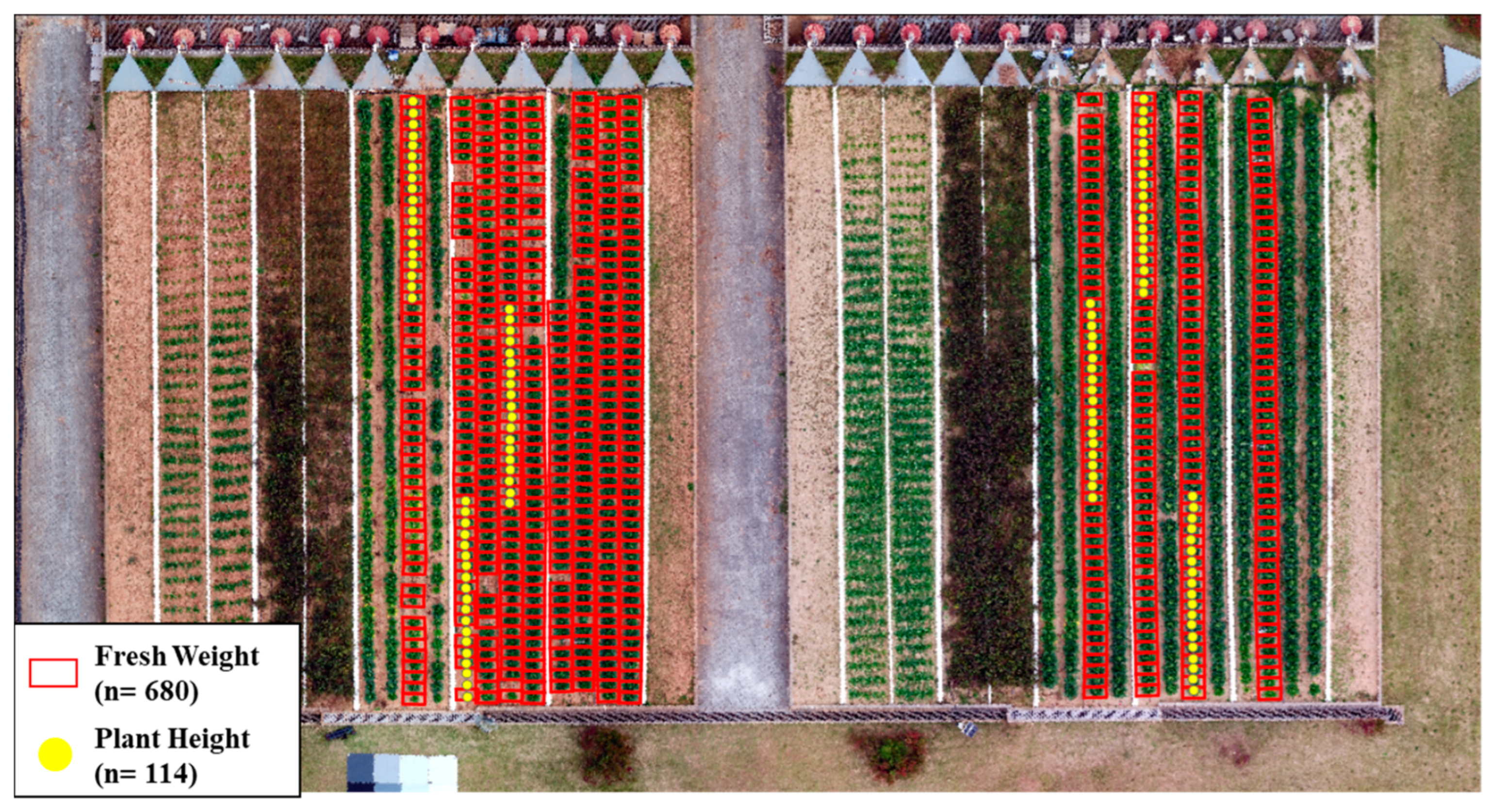
Field surveys were conducted to measure plant height and fresh weight, two key indicators of Napa cabbage growth. Plant height was determined by measuring the distance from the ground to the highest leaf at each survey time point. A subset of 114 Napa cabbages was selected for draft measurements to compare with model predictions. To maintain consistency, both UAS image acquisition and Napa cabbage draft surveys were conducted on the same day. The specific locations of these 114 sampled Napa cabbages are indicated by yellow dots in Figure 6.
On 9 November 2020, the final harvest date, the fresh weights of 680 Napa cabbages were measured. For these Napa cabbages, both location information and fresh weight were recorded, forming a comprehensive dataset. Additionally, the fresh weights of 625 Napa cabbages not selected as samples were measured randomly, albeit without location information. The spatial distribution of the 680 georeferenced Napa cabbage samples is illustrated by red boxes in Figure 6.
The data collected through these field surveys served as ground truth for training and evaluating the AI models developed to predict Napa cabbage fresh weight.

2.7. Individual Napa Cabbage Object Segmentation

To analyze individual Napa cabbage plants, it is necessary to segment the cabbage objects. This study utilized the Excess Green (ExG) index, Otsu’s thresholding method, and grid generation techniques to achieve this segmentation.

2.7.1. Vegetation Segmentation Using ExG and Otsu Methods

The ExG vegetation index [37], calculated as ExG = 2G − R − B (where R, G, and B represent reflectance values in the red, green, and blue bands, respectively), was utilized in this study to enhance the contrast between vegetation and background elements in RGB images captured by the Zenmuse X5s camera mounted on the Inspire 2 UAS. This index leverages the principle that healthy vegetation reflects more green light than red or blue light, resulting in positive ExG values for green vegetation and negative values for non-green areas like soil or water. Higher positive ExG values generally correlate with healthier vegetation.
In this study, a custom Python (version 3.8.8) script was employed to extract ExG images from the RGB imagery. These ExG images served as valuable inputs for generating additional vegetation indices, which were subsequently used as features in the AI models for fresh weight prediction. The utilization of ExG images proved advantageous due to their simple calculation, relative insensitivity to varying illumination and atmospheric conditions, ability to differentiate vegetation types based on spectral reflectance, and proven effectiveness in various agricultural applications such as crop monitoring, yield prediction, and weed detection. By providing a clear distinction between Napa cabbage plants and the background soil, ExG enhanced the models’ ability to focus on relevant features, leading to more accurate and precise fresh weight predictions.

2.7.2. Otsu’s Method for Image Segmentation

Otsu’s method, a widely used, non-parametric, and unsupervised image segmentation algorithm [38], was employed to distinguish foreground (Napa cabbage plants) from background (soil) in grayscale images. This method maximizes the inter-class variance (σ2_B), a measure of dissimilarity between the two classes, to determine an optimal threshold.
The inter-class variance at a given threshold t is calculated as:
σ2_B(t) = ω_0(t) × σ2_0(t) + ω_1(t) × σ2_1(t)
where, ω_0(t) and ω_1(t) represent the weights (proportional to the number of pixels) of the background and foreground classes, respectively, at threshold t. σ2_0(t) and σ2_1(t) represent the variances of the background and foreground classes, respectively, at threshold t.
The optimal threshold (t*) is determined by iterating over all possible threshold values and selecting the one that maximizes the inter-class variance, as shown in Equation (2):
t* = argmax σ2_B(t)
In this study, Otsu’s method was applied to grayscale versions of the ExG images derived from UAS-captured RGB imagery to segment individual Napa cabbage plants from the background soil. The resulting binary images facilitated the accurate calculation of vegetation indices and other features, which were essential inputs for the AI models used to predict Napa cabbage fresh weight. This automatic segmentation process proved crucial for precise feature extraction, ultimately contributing to the successful prediction of Napa cabbage fresh weight.

2.7.3. Process of Individual Napa Cabbage Object Segmentation

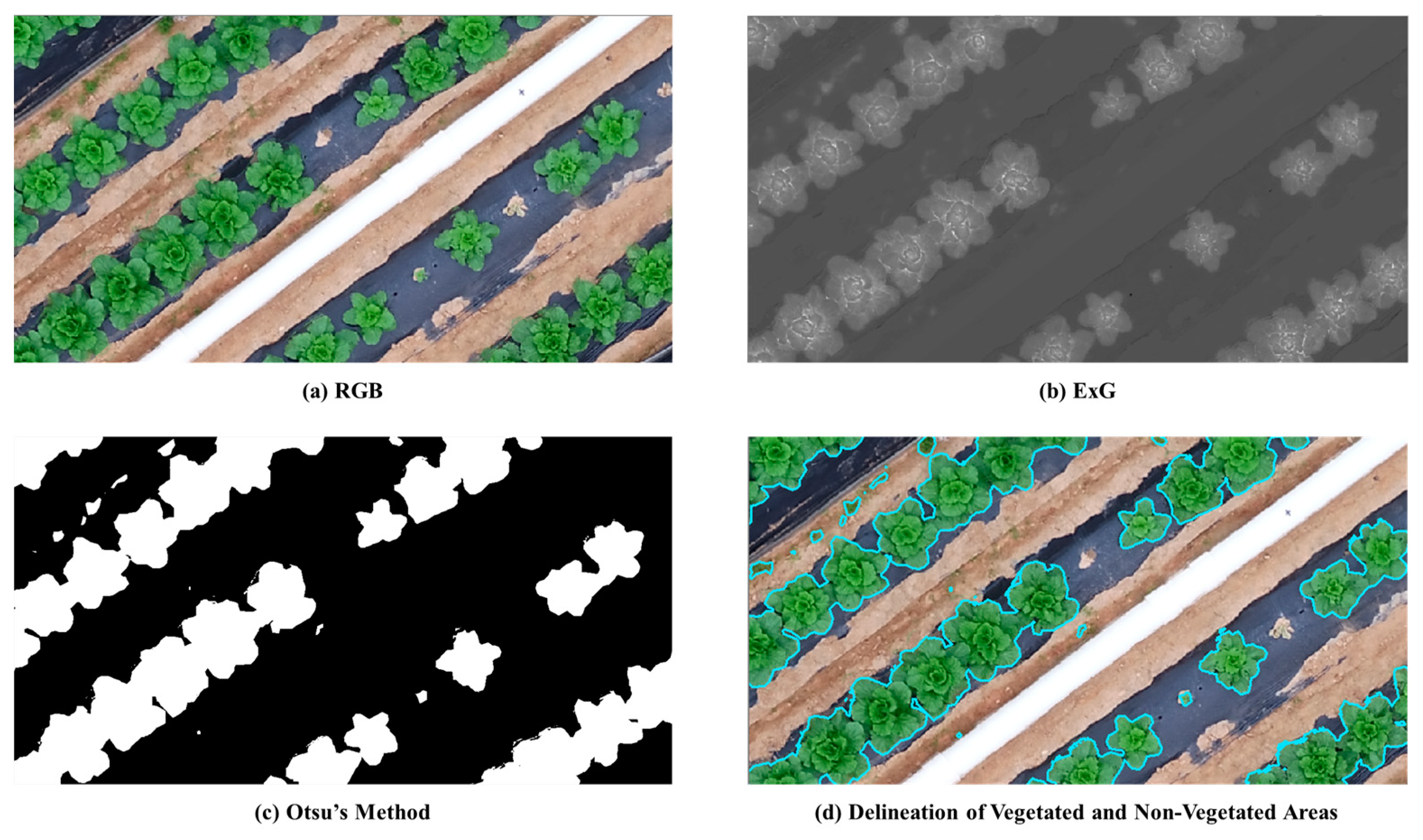
Individual Napa cabbage objects were segmented from UAS imagery using a multi-step process (Figure 7).
First, RGB images (Figure 7a) were converted to ExG indices to enhance the contrast between vegetation and background (Figure 7b). Otsu’s thresholding method was then applied to the ExG images, generating binary masks that differentiated vegetation from non-vegetation areas (Figure 7c). Here, the ‘vegetation area’ refers to the two-dimensional planar area occupied by the cabbage canopy as observed in the UAS imagery. These binary masks were then vectorized, retaining only the vegetated regions, resulting in precise outlines of individual Napa cabbage plants (Figure 7d).
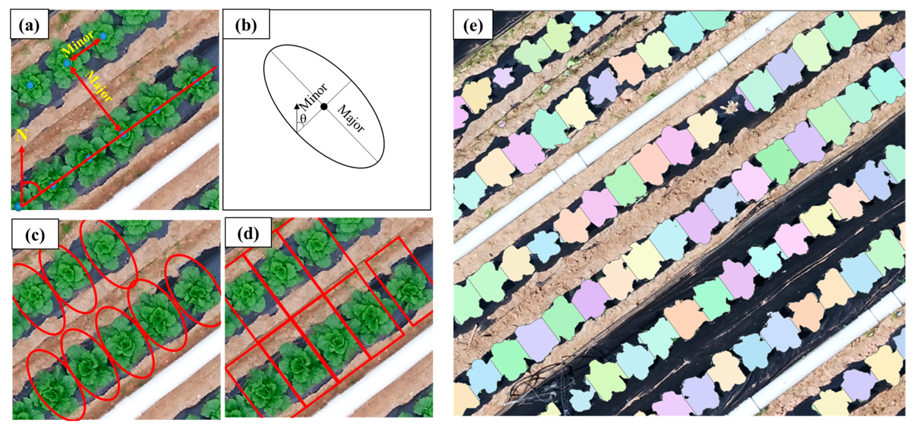
However, due to the overlapping nature of Napa cabbage plants during the rosette growth stage, the initial segmentation often grouped multiple plants as a single object. To address this, a grid-based approach was implemented in ArcGIS Pro (Esri, Redlands, CA, USA), version 2.9, to delineate individual plants (Figure 8). First, the center point of each Napa cabbage object was digitized (Figure 8a). An ellipse was then generated around each point, with major and minor axes corresponding to the valley and planting spacing, respectively, and the angle θ representing the row orientation relative to true north (Figure 8b). These ellipses were adjusted to match the actual location of each Napa cabbage plant within the row, resulting in distorted ellipses aligned with the true north direction (Figure 8c). The ellipses were then converted into inscribed rectangular grids (Figure 8d), which were used to separate the overlapping Napa cabbage vector data, enabling the final segmentation of individual Napa cabbage objects (Figure 8e).
The segmented object areas were used to extract individual growth information for each Napa cabbage plant, such as vegetation indices, crop height, and canopy cover. This information served as crucial input features for the subsequent fresh weight prediction models.

2.8. Definition of Independent Variables for AI Models

The independent variables for the AI algorithms predicting Napa cabbage fresh weight were derived from a multi-sensor approach, incorporating RGB, MSP, and TIR imagery.

2.8.1. RGB-Based Independent Variables

Two variables representing the physical characteristics of Napa cabbage were selected from the RGB imagery.
Vegetation Fraction (VF; 2D planar area): the ratio of the area occupied by each Napa cabbage plant (Figure 8) to the grid area corresponding to the plant (Figure 8d), calculated as:
VF = (Area of each Napa cabbage object)/(Grid area)
Crop Height Model (CHM): the height of each Napa cabbage plant was estimated using the difference between the Digital Surface Model (DSM) at each growth stage and the DSM before planting, leveraging the Structure from Motion (SfM) algorithm:
CHM = DSM_(growth stage) − DSM_(pre-planting)
This approach, utilizing RGB imagery and the derived DSM, facilitated the analysis of the Napa cabbage objects’ cross-sectional area and vegetation height, thereby enabling the investigation of their 3D structural characteristics. The use of 2D cross-sectional areas and DSMs has been instrumental in estimating structural features in various crops, including wheat, Napa cabbage, and radish [21,32]. By leveraging these data, we can gain more accurate insights into the growth patterns and physical dimensions of these crops.

2.8.2. Multispectral Sensor-Based Independent Variables

Eight vegetation indices (VIs) known to correlate with leaf chlorophyll content (LCC), a crucial indicator of crop nitrogen status and yield, were selected based on preliminary experiments [30] and derived from the MSP imagery. These indices, detailed in Table 2, were chosen for their established relationships with chlorophyll content and their potential to provide valuable insights into cabbage growth and development.

2.8.3. Thermal Infrared Sensor-Based Independent Variable

The Crop Water Stress Index (CWSI), a measure of plant water stress, was selected as the TIR-based variable. CWSI was calculated using the formula proposed by Jones [39], which utilizes only UAS-based TIR images:
CWSI = (TTc)/(ThTc)
where, T is the temperature of individual pixels in the TIR image, Tc is the lowest temperature within the vegetation area, and Th is the highest temperature within the vegetation area.
To ensure accurate CWSI calculation, only vegetation pixel temperatures were utilized, as determined using vector data delineating Napa cabbage areas.
For each of the 680 sampled Napa cabbage individuals, the average value of each independent variable within the plant’s designated grid area was used as the input for the AI models. This multi-sensor approach aimed to capture the diverse aspects of Napa cabbage growth and physiology, thereby enhancing the predictive power of the fresh weight models.
Table 2. Vegetation indices and crop features extracted from UAS multi-sensor data for Napa cabbage fresh weight prediction.
Sensor TypeVegetation IndexEquationReference
RGBVF (Vegetation Fraction)VF = (Area of each Napa cabbage object)/(Grid area)-
CHM (Crop Height Model)CHM = DSM_(growth stage) − DTM_(pre-planting)[21]
Multi
Spectral
CIRE
(Red Edge Chlorophyll Index)
CIRE = (RN/RRE) − 1[40]
VARI
(Visible Atmospherically Resistant Index)
VARI = (RG − RR)/(RG + RR)[41]
CVI (Chlorophyll Vegetation Index)CVI = (RN/RG) × (RR/RG)[42]
SR (Simple Ratio)SR = (RN/RG)[43]
GNDVI
(Green Normalized Difference
Vegetation Index)
GNDVI = (RN − RG)/(RN + RG)[44]
CIGreen
(Green Chlorophyll Index)
CIGreen = (RN/RG) − 1[40]
GEMI
(Global Environmental
Monitoring Index)
GEMI = n × [(1 − 0.25n) × (RR − 0.125)]/(1 − RR)
n = [(RN2 − RR2) + 1.5 × RN + 0.5 × RR]/(RN + RR + 0.5)
[45]
NDVI
(Normalized Difference
Vegetation Index)
NDVI = (RN − RR)/(RN + RR)[46]
Thermal
Infrared
CWSI
(Crop Water Stress Index)
CWSI = (T − Tc)/(Th − Tc)[39]

2.9. Construction of Datasets and AI Models

The collected dataset, comprising 680 data points, was randomly partitioned into training (70%, 476 points) and testing (30%, 204 points) sets for hyperparameter tuning, training, and testing of the AI algorithms.
This study employed three algorithms for predicting Napa cabbage fresh weight: DNN, SVM, and RF. The DNN model, analogous to the artificial neural network (ANN) algorithm, was structured with an input layer incorporating 11 independent variables (defined in Section 2.8), followed by three hidden layers with 128, 64, and 32 nodes, respectively (Figure 9). The output layer yielded the predicted Napa cabbage fresh weight. The ReLU activation function, chosen for its computational efficiency and ability to mitigate the vanishing gradient problem, was employed for non-linear modeling. Optimization of the loss function was achieved using the Adam optimizer. To identify the optimal prediction time, seven DNN models were created, each trained on data from a specific period between 10 September and 27 October 2020, and their predictive accuracy was compared.
For performance comparison, SVM and RF models were also constructed. The SVM algorithm utilized the radial basis function (RBF) kernel, with hyperparameters C and gamma optimized [47]. For the RF algorithm, the ‘mtry’ hyperparameter (number of variables randomly sampled as candidates at each split) was tuned [48]. Model validation was rigorously performed using five-fold cross-validation on 70% of the training data, repeated five times to ensure robustness and to assess generalization capability.

2.10. Accuracy Evaluation

2.10.1. Model Accuracy Evaluation

The accuracy of Napa cabbage fresh weight prediction was assessed using two metrics: the coefficient of determination (R2) and the root mean square error (RMSE). R2 quantifies the proportion of variance in the observed fresh weights explained by the model, while RMSE measures the average magnitude of the prediction errors. These metrics were calculated using the following formulas:
R2 = 1 − 1 − (SSE/SST)
R M S E = ( y i y ^ i ) 2 n
where, SSE (Sum of Squared Errors) is the sum of the squared differences between the observed values ( y i ) and the predicted values ( y ^ i ), SST (Total Sum of Squares) is the sum of the squared differences between the observed values ( y i ) and the mean of the observed values (ȳ), and n is the total number of samples.
R2 represents the proportion of the variance in the dependent variable (Napa cabbage fresh weight) that is predictable from the independent variables (the features extracted from the UAS imagery). A value of R2 close to 1 indicates a good fit of the model, while a value close to 0 indicates a poor fit. The RMSE is a measure of the average magnitude of the errors in a set of predictions. RMSE quantifies the average deviation between the predicted and actual fresh weights of cabbages. A lower RMSE value indicates better predictive accuracy, as the predicted values are closer to the observed values.

2.10.2. Feature Importance

To evaluate the importance of features, the permutation feature importance (PFI) method was employed [49]. PFI measures the decrease in model accuracy (e.g., RMSE) when a single feature’s values are randomly shuffled. A larger decrease signifies a more important feature, as its disruption impacts the model’s predictive capability more significantly. In this study, the PFI algorithm was applied to the DNN model optimized for predicting fresh weight at the most suitable growth stage (DAP 42), allowing for a quantitative assessment of each feature’s contribution to the model’s performance.

3. Results

3.1. Model Accuracy Evaluation by Survey Period

The performance of three AI models (DNN, SVM, and RF) in predicting Napa cabbage fresh weight was evaluated using multi-sensor fusion data acquired from UAS flights on seven dates between 10 September and 27 October 2020 (Table 3).
The DNN model consistently outperformed the SVM and RF models across all survey dates for both training and test datasets, as evidenced by higher R2 values and lower RMSE values (Figure 10 and Figure 11). Notably, the DNN model achieved the highest accuracy (R2 = 0.82, RMSE = 0.47 kg) on October 13 (DAP 42), coinciding with the mid-rosette growth stage. In Table 3, the asterisk (*) is used to highlight the model with the highest R² value among all models and datasets for a given survey date. The RF model showed the lowest performance, particularly on the test dataset, suggesting potential overfitting.
The overall model performance, as indicated by R2, generally improved as the Napa cabbage growth progressed. The lowest R2 values were observed in the early growth stages (DAP 9–14), followed by a gradual increase and a sharp rise on October 6 (DAP 35). This trend suggests that the predictive ability of the models improved as the Napa cabbage plants matured and developed distinct morphological features, with the DNN model being particularly adept at capturing this progression.
The consistent R2 values for the DNN model between training and test datasets highlight its robustness and generalizability. In contrast, the lower R2 values of SVM and RF, particularly in the test dataset, indicate potential overfitting to the training data. The RMSE values further substantiate the DNN model’s superior performance, consistently exhibiting the lowest prediction errors across all survey dates.
The observed superiority of the DNN model can be attributed to its deep, layered architecture, making it more capable of capturing the complex, non-linear relationships between Napa cabbage fresh weight and the multi-sensor features extracted from UAS imagery. The model’s ability to learn and represent these intricate relationships contributes to its higher predictive accuracy, especially as the Napa cabbage plants mature and exhibit more distinct features during the mid-to-late rosette stage.

3.2. Model Overfitting Analysis

To assess the generalization ability of the three AI models, an overfitting analysis was conducted by comparing their performance metrics (R2 and RMSE) on the training and test datasets (Figure 12). Greater discrepancies between the metrics for the two datasets indicate a higher degree of overfitting.
The DNN model exhibited exceptional stability across all growth stages (DAP 9–56), with minimal variation in both R2 and RMSE differences between the training and test datasets, suggesting good generalization. In contrast, the RF model exhibited the most significant fluctuations in R2 and RMSE differences, particularly in the later growth stages (DAP 35–56), signifying a higher degree of overfitting. The SVM model showed moderate overfitting, with differences generally falling between those of the DNN and RF models.
Quantitatively, the DNN model’s minimal overfitting was evident in the small discrepancies between training and test metrics: R2 differences ranged from 0.013 to 0.028, and RMSE differences from 0.025 to 0.054 kg. The SVM model showed slightly larger differences, with R2 ranging from 0.017 to 0.049, and RMSE from 0.033 to 0.094 kg. The RF model exhibited the most pronounced overfitting, with R2 differences ranging from 0.065 to 0.148, and RMSE differences from 0.125 to 0.285 kg.
Overall, the analysis indicates that the DNN model is the most robust and least prone to overfitting among the three models tested, making it the most suitable choice for predicting Napa cabbage fresh weight in this study.

3.3. Fresh Weight Prediction Performance of DNN, SVM, and RF Models

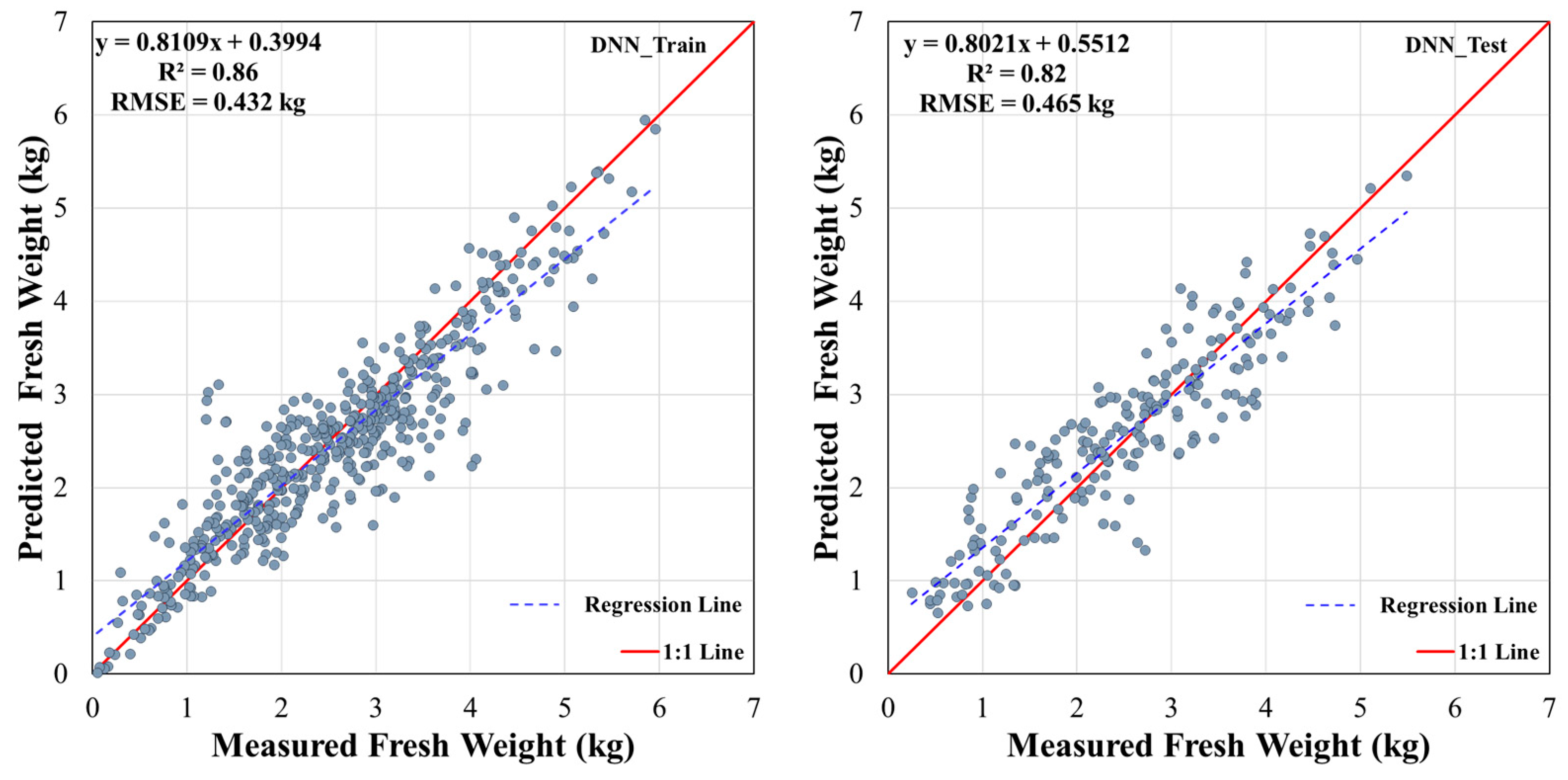
Figure 13, Figure 14 and Figure 15 present scatter plots comparing the predicted and measured fresh weights of individual Napa cabbage heads for the DNN, SVM, and RF models, respectively, using the model from 13 October 2020 (DAP 42).
The DNN model (Figure 13) demonstrated the highest accuracy and generalizability, consistently achieving high R2 values (0.86 for training and 0.82 for testing) and low RMSE values (0.432 kg for training and 0.465 kg for testing) across both datasets. The close alignment of the regression lines with the 1:1 line further indicates a strong positive correlation between predicted and measured fresh weights.
The SVM model (Figure 14) showed good predictive performance on the training dataset (R2 = 0.78, RMSE = 0.546 kg), comparable to the DNN model. However, there was a slight decrease in accuracy and evidence of minor overfitting on the test dataset (R2 = 0.73, RMSE = 0.544 kg).
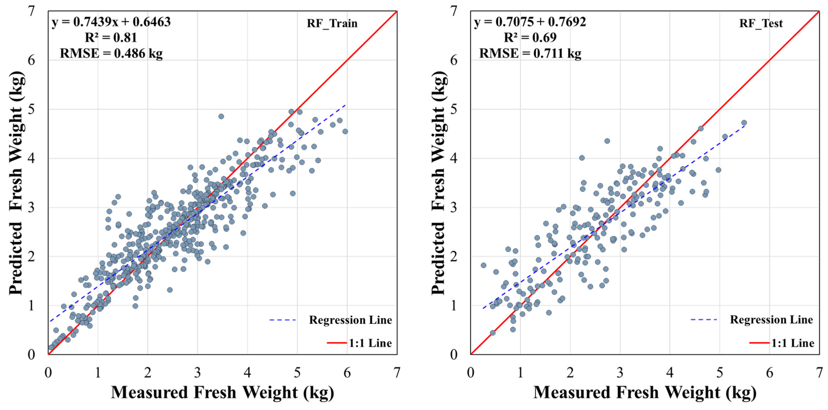
The RF model (Figure 15) exhibited the lowest performance among the three models. While it showed a good correlation on the training dataset (R2 = 0.81, RMSE = 0.486 kg), its accuracy significantly decreased on the test dataset (R2 = 0.69, RMSE = 0.711 kg), indicating overfitting.
In summary, the DNN model proved to be the most accurate and robust model for predicting Napa cabbage fresh weight, followed by the SVM model with slightly lower accuracy. The RF model, while performing well on the training data, exhibited the highest degree of overfitting and the lowest overall accuracy.

3.4. Bias Analysis for Overall and Fresh Weight Sections of DNN, SVM, and RF Models

Table 4 presents the fresh weight bias analysis for the DNN, SVM, and RF models, comparing predicted and measured values for both overall Napa cabbage weight and individual weight sections (head, stem, inner leaves, outer leaves, and total leaves). A negative bias indicates overestimation, while a positive bias signifies underestimation.
The DNN model demonstrates the highest accuracy in predicting total Napa cabbage fresh weight, exhibiting the lowest overall bias (0.008 kg). The DNN model tends to overestimate for cabbages weighing less than 2 kg and underestimate for those exceeding 2 kg. Conversely, the RF and SVM models generally overestimate for cabbages under 3 kg and underestimate for those over 3 kg, with overall biases of 0.031 kg and 0.041 kg, respectively.
Across individual weight sections, the DNN model consistently exhibits the lowest bias, except for the leaf section, where the SVM model demonstrates a marginally lower bias (0.004 kg) compared to the DNN model (0.003 kg). However, the RF model consistently exhibits the highest bias across all weight sections, indicating its lower accuracy in predicting individual component weights.
The bias analysis further reveals the following model-specific patterns:
  • DNN: The highest bias (underestimation of 0.365 kg) is observed in the 4–5 kg range.
  • RF: The highest bias (underestimation of 0.541 kg) occurs for Napa cabbages exceeding 5 kg.
  • SVM: Similar to the RF model, the highest bias (underestimation of 0.88 kg) is also observed in the >5 kg range.
These findings underscore the importance of considering model-specific biases and the weight range of the Napa cabbages when selecting the most appropriate model for fresh weight prediction. The DNN model is generally the most accurate, but the SVM model may be slightly more suitable for predicting leaf weight. Furthermore, the RF model may require further refinement to improve its predictive accuracy, especially for heavier Napa cabbages.

3.5. Evaluation of Feature Importance in DNN, SVM, and RF Models Using Permutation Feature Importance (PFI)

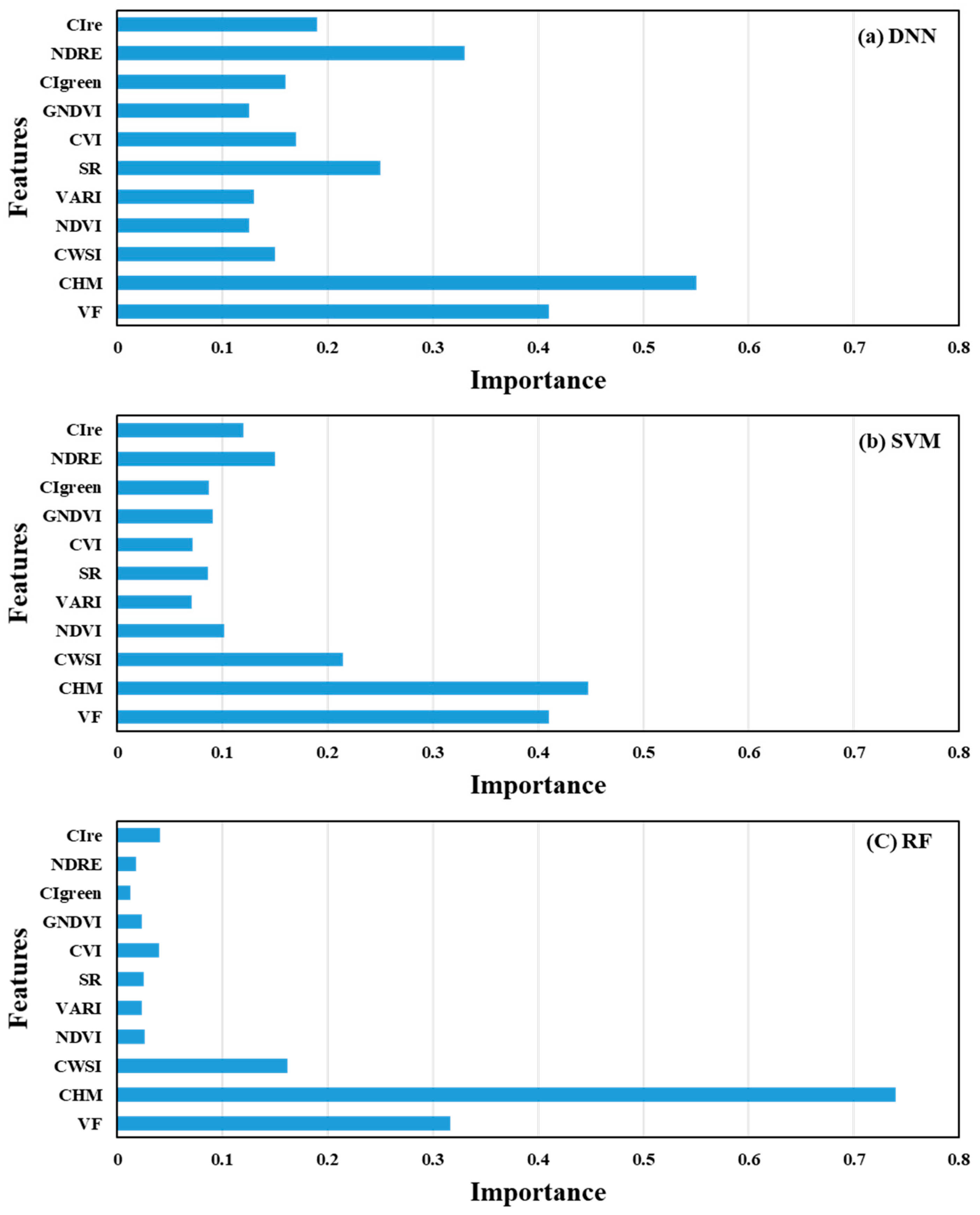
To assess the influence of each variable on fresh weight prediction, the PFI algorithm was employed using data from 13 October 2020 (DAP 42), identified as the optimal growth stage. As shown in Figure 16, all three models (DNN, SVM, and RF) highlighted CHM and VF (2D planar area) as the most significant variables.
In the DNN model, CHM and VF were identified as the top variables, with the NDRE index also showing a significant contribution. The SVM model also emphasized CHM and VF, but showed a higher importance for the CWSI derived from the TIR sensor. In contrast, the RF model maintained a strong preference for CHM and VF, with minimal contributions from other vegetation indices. This analysis demonstrates the differing levels of reliance on various indices across the three models, with each model prioritizing features differently based on their underlying algorithms and data processing approaches.

3.6. Spatial Analysis of Measured and Predicted Napa Cabbage Fresh Weight Using the DNN Model

3.6.1. Comparison of Spatial Distributions and Weight Category Frequencies

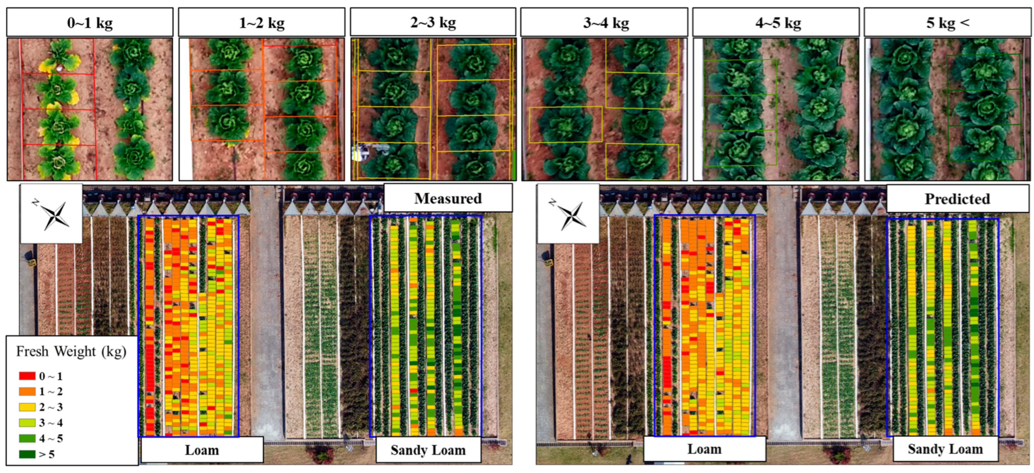
Figure 17 illustrates the spatial distribution of both measured and DNN model-predicted Napa cabbage fresh weights on 13 October 2020 (DAP 42). The test field was divided into two distinct plots: loam (left) and sandy loam (right). The top panels in Figure 17 display the measured fresh weights, while the bottom panels showcase the corresponding DNN model predictions. The color gradient represents the fresh weight range, with red signifying the lowest weights (<1 kg) and purple the highest (>5 kg). The spatial distribution of predicted fresh weights closely mirrored the observed patterns in the measured weights, underscoring the DNN model’s capability to capture spatial variability across soil types and irrigation regimes.
Figure 17 also visually reinforces the substantial influence of soil type and irrigation on cabbage fresh weight. The non-irrigated loam plot predominantly exhibited lower fresh weights, with most cabbages falling within the 0–3 kg range, reflecting the impact of water stress on growth. In contrast, the irrigated sandy loam plot displayed a more uniform and wider distribution of fresh weights, with a greater proportion of cabbages in the 3–5 kg range, highlighting the beneficial effect of irrigation on yield.

3.6.2. Overall Model Performance and Spatial Variability

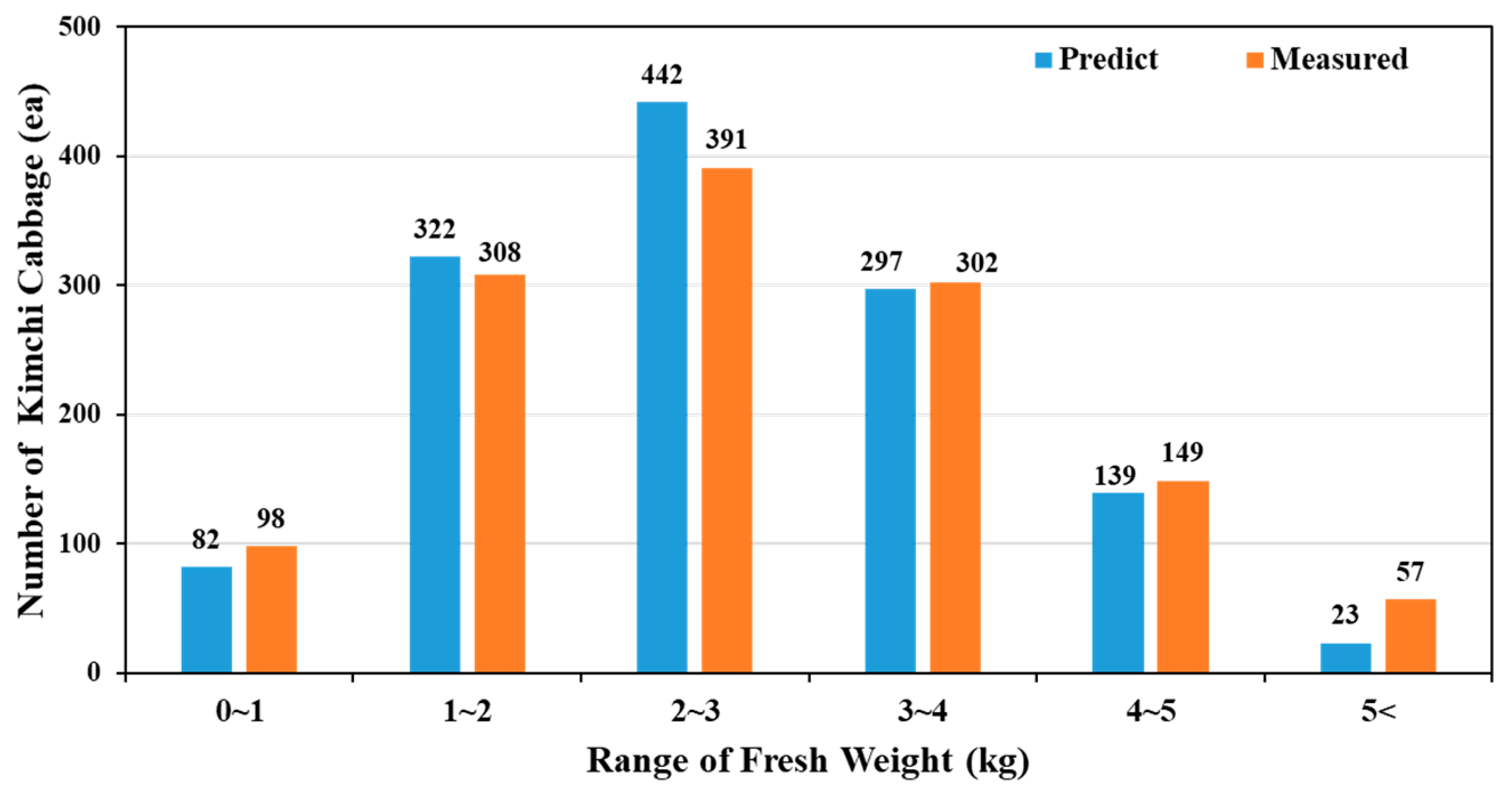
Figure 18 provides a more quantitative comparison of the predicted and measured fresh weight distributions, categorized into six weight classes. The DNN model demonstrated good agreement with the measured data, especially for cabbages weighing 1–2 kg and 3–4 kg. However, some discrepancies were observed in the 2–3 kg and >5 kg ranges, suggesting potential areas for further model refinement. The model tended to overestimate the number of cabbages in the 2–3 kg range and underestimate those exceeding 5 kg.
Table 5 presents a comprehensive comparison of the measured and predicted total fresh weights for all 1305 harvested cabbages from both loam and sandy loam plots. The DNN model achieved a low error rate of 2.69%, highlighting its overall effectiveness in predicting fresh weight across the entire test field.
These spatial analyses collectively demonstrate the DNN model’s capability to accurately predict Napa cabbage fresh weight and capture the spatial variability arising from differences in soil type and irrigation practices. The model’s performance, while generally strong, also highlights the need for further refinement in specific weight ranges and under varying environmental conditions. Nevertheless, the results of this study demonstrate the promising potential of UAS-based multi-sensor data and deep learning algorithms for enhancing precision agriculture and improving cabbage yield prediction.

4. Discussion

This study investigated the application of three AI algorithms (DNN, SVM, and RF) to predict Napa cabbage fresh weight using UAS-based multi-sensor data. The DNN model, particularly when trained on data collected during the heading stage (DAP 42), demonstrated superior accuracy and stability. This suggests that the canopy’s structural characteristics at this stage, characterized by increased leaf number and stable leaf area, serve as robust predictors of final fresh weight.
While the model trained on DAP 35 (also within the heading stage) performed well, it was slightly less accurate than the DAP 42 model. This discrepancy may be attributed to individual variations in growth rate, as some plants may still be actively growing in terms of leaf number and area at this earlier time point.
The prediction accuracy decreased slightly for the model trained on DAP 56, closer to harvest. This reduction might be due to the senescence of outer leaves and reduced photosynthetic capacity, impacting the vegetation indices and, consequently, fresh weight prediction. The lowest accuracy was observed for the model trained during the seedling stage (DAP 9). The numerous variables influencing growth until harvest make fresh weight prediction challenging during this early stage.
The variation in model performance across growth stages is linked to the changing factors influencing Napa cabbage growth. The PFI analysis indicated that CHM and VF were the most influential variables, reflecting the significance of physical characteristics, particularly after outer leaf removal, in determining final fresh weight. These physical factors proved more critical than vegetation indices or water stress indicators. Among the vegetation indices, those utilizing the Red Edge band (e.g., NDRE and CIre) were generally more important than others. This is likely because indices like NDVI tend to saturate in late growth stages, while Red Edge-based indices remain sensitive to changes in chlorophyll concentration [50,51].
The PFI results also revealed that the RF model’s heavy reliance on CHM and VF contributed to its lower accuracy, overfitting, and bias. In contrast, SVM and DNN models incorporated a wider range of variables, leading to more consistent accuracy between training and test sets. Notably, DNN consistently outperformed SVM and RF in various studies, including those involving potatoes, corn, camellia, wheat, and soybeans [31,52,53,54], a trend also observed in this study.
While the DNN model excelled overall, it tended to underestimate the weight of cabbages exceeding 5 kg. This may be attributed to the limited representation of large cabbages in the dataset and the saturation of vegetation indices at high chlorophyll concentrations, hindering the model’s ability to differentiate between these individuals. However, the model accurately predicted the fresh weight of smaller cabbages, offering valuable insights for yield prediction and identifying underperforming plants.
A limitation of the current model is its reliance on single time-point data, which may not fully capture the continuous growth patterns and temporal dynamics of the crop. This could lead to less accurate predictions, particularly for larger cabbages or under varying environmental conditions. Future research should investigate incorporating models like CNN-LSTM, which can effectively capture temporal changes in features, potentially improving prediction accuracy across different growth stages and environments.
Overall, this study highlights the potential of UAS-based multi-sensor data and AI, specifically the DNN model, for the accurate and non-invasive prediction of Napa cabbage fresh weight. The findings emphasize the importance of the heading stage for fresh weight estimation and underscore the need for further research to address model limitations and enhance its applicability to a broader range of agricultural scenarios.

5. Conclusions

This study successfully developed and evaluated AI models for predicting Napa cabbage fresh weight using UAS-based multi-sensor data. The DNN model consistently outperformed SVM and RF models, achieving its highest accuracy (R2 = 0.82, RMSE = 0.47 kg) during the mid-to-late rosette growth stage (35–42 DAP). This suggests that canopy structural characteristics at this stage are robust predictors of final fresh weight. The model’s improving accuracy as cabbages matured highlights the heading stage’s importance for fresh weight estimation.
The DNN model effectively captured spatial variability in cabbage growth due to soil type and irrigation, accurately reflecting the positive impact of drip irrigation on the sandy loam plot. However, the model tended to underestimate the weight of cabbages exceeding 5 kg, potentially due to limited large cabbage samples and saturation effects of vegetation indices at high chlorophyll concentrations. Despite this, the overall error rate was less than 5%, demonstrating the feasibility and effectiveness of the proposed approach.
This research significantly contributes to precision agriculture by showcasing the potential of UAS-based multi-sensor data and AI algorithms for the accurate and non-invasive prediction of Napa cabbage fresh weight. The developed DNN model offers a valuable tool for optimizing harvest timing, improving crop management practices, and enhancing supply chain efficiency. By enabling early and precise yield estimation, this technology empowers farmers to make informed decisions, ultimately leading to increased profitability and reduced food waste.
Future research should focus on addressing the limitations identified in this study. This includes improving the prediction accuracy for larger cabbages, potentially by expanding the dataset to include more diverse samples and exploring advanced AI techniques that better handle feature saturation. Additionally, the model’s applicability to other crops and varying environmental conditions should be investigated, further broadening its potential impact on sustainable agriculture.

Author Contributions

Conceptualization, D.-H.L.; methodology, D.-H.L. and J.-H.P.; software, D.-H.L.; validation, J.-H.P.; formal analysis, D.-H.L.; investigation, D.-H.L. and J.-H.P.; resources, D.-H.L. and J.-H.P.; data curation, D.-H.L.; writing—original draft preparation, D.-H.L.; writing—review and editing, J.-H.P.; visualization, D.-H.L.; supervision, J.-H.P. All authors have read and agreed to the published version of the manuscript.

Funding

This research received no external funding.

Data Availability Statement

The data presented in this study are available on request from the corresponding author. The data are not publicly available due to privacy concerns.

Conflicts of Interest

The authors declare no conflicts of interest.

References

  1. Lobell, D.B.; Schlenker, W.; Costa-Roberts, J. Climate Trends and Global Crop Production since 1980. Science 2011, 333, 616–620. [Google Scholar] [CrossRef] [PubMed]
  2. Walsh, K.J.; McBride, J.L.; Klotzbach, P.J.; Balachandran, S.; Camargo, S.J.; Holland, G.; Knutson, T.R.; Kossin, J.P.; Lee, T.; Sobel, A. Tropical Cyclones and Climate Change. Wiley Interdiscip. Rev. Clim. Change 2016, 7, 65–89. [Google Scholar] [CrossRef]
  3. Ummenhofer, C.C.; Meehl, G.A. Extreme Weather and Climate Events with Ecological Relevance: A Review. Philos. Trans. R. Soc. B. 2017, 372, 20160135. [Google Scholar] [CrossRef] [PubMed]
  4. Sishodia, R.P.; Ray, R.L.; Singh, S.K. Applications of Remote Sensing in Precision Agriculture: A Review. Remote Sens. 2020, 12, 3136. [Google Scholar] [CrossRef]
  5. Kwaghtyo, D.K.; Eke, C.I. Smart Farming Prediction Models for Precision Agriculture: A Comprehensive Survey. Artif. Intell. Rev. 2023, 56, 5729–5772. [Google Scholar] [CrossRef]
  6. Kim, I.; Jeong, S.; Jeong, G. An Analysis of the Impact of Changes in Kimchi Imports on the Korean Kimchi Industry. Korean J. Org. Agric. 2022, 30, 151–170. [Google Scholar] [CrossRef]
  7. Eum, H.L.; Kim, B.; Yang, Y.J.; Hong, S.J. Quality Evaluation and Optimization of Storage Temperature with Eight Cultivars of Kimchi Cabbage Produced in Summer at Highland Areas. Hortic. Sci. Technol. 2013, 31, 211–218. [Google Scholar] [CrossRef]
  8. Choi, E.J.; Jeong, M.C.; Ku, K.H. Effect of Seasonal Cabbage Cultivar (Brassica rapa L. Ssp. Pekinesis) on the Quality Characteristics of Salted-Kimchi Cabbages during Storage Period. Korean J. Food Preserv. 2015, 22, 303–313. [Google Scholar] [CrossRef]
  9. Radoglou-Grammatikis, P.; Sarigiannidis, P.; Lagkas, T.; Moscholios, I. A Compilation of UAV Applications for Precision Agriculture. Comput. Netw. 2020, 172, 107148. [Google Scholar] [CrossRef]
  10. Tripathi, M.K.; Maktedar, D.D. A Role of Computer Vision in Fruits and Vegetables among various Horticulture Products of Agriculture Fields: A Survey. Inf. Process. Agric. 2020, 7, 183–203. [Google Scholar] [CrossRef]
  11. De Ocampo, A.L.P.; Montalbo, F.J.P. A Multi-Vision Monitoring Framework for Simultaneous Real-Time Unmanned Aerial Monitoring of Farmer Activity and Crop Health. Smart Agric. Technol. 2024, 8, 100466. [Google Scholar] [CrossRef]
  12. Mezera, J.; Lukas, V.; Horniaček, I.; Smutný, V.; Elbl, J. Comparison of Proximal and Remote Sensing for the Diagnosis of Crop Status in Site-Specific Crop Management. Sensors 2021, 22, 19. [Google Scholar] [CrossRef] [PubMed]
  13. Kumar, H.; Srivastava, P.; Lamba, J.; Ortiz, B.V.; Way, T.R.; Sangha, L.; Takhellambam, B.S.; Morata, G.; Molinari, R. Within-Field Variability in Nutrients for Site-Specific Agricultural Management in Irrigated Cornfield. J. ASABE 2022, 65, 865–880. [Google Scholar] [CrossRef]
  14. Flores, R.; Lázaro, E.; Ramos, E.; Provost, K.; Habib, M. Demand Management in the Supply Chain: A Focus on Agribusiness. In Advances in Manufacturing, Production Management and Process Control: Proceedings of the AHFE 2020 Virtual Conferences on Human Aspects of Advanced Manufacturing, Advanced Production Management and Process Control, and Additive Manufacturing, Modeling Systems and 3D Prototyping, San Diego, CA, USA, 16–20 July 2020; Springer: Cham, Switzerland, 2020; pp. 333–340. [Google Scholar]
  15. Karthikeyan, L.; Chawla, I.; Mishra, A.K. A Review of Remote Sensing Applications in Agriculture for Food Security: Crop Growth and Yield, Irrigation, and Crop Losses. J. Hydrol. 2020, 586, 124905. [Google Scholar] [CrossRef]
  16. Shi, Y.; Ji, S.; Shao, X.; Tang, H.; Wu, W.; Yang, P.; Zhang, Y.; Ryosuke, S. Framework of SAGI Agriculture Remote Sensing and its Perspectives in Supporting National Food Security. J. Integr. Agric. 2014, 13, 1443–1450. [Google Scholar] [CrossRef]
  17. Saranya, T.; Deisy, C.; Sridevi, S.; Anbananthen, K.S.M. A Comparative Study of Deep Learning and Internet of Things for Precision Agriculture. Eng. Appl. Artif. Intell. 2023, 122, 106034. [Google Scholar] [CrossRef]
  18. Benos, L.; Tagarakis, A.C.; Dolias, G.; Berruto, R.; Kateris, D.; Bochtis, D. Machine Learning in Agriculture: A Comprehensive Updated Review. Sensors 2021, 21, 3758. [Google Scholar] [CrossRef]
  19. Lee, D.; Shin, H.; Park, J. Developing a P-NDVI Map for Highland Kimchi Cabbage using Spectral Information from UAVs and a Field Spectral Radiometer. Agronomy 2020, 10, 1798. [Google Scholar] [CrossRef]
  20. Zhang, C.; Kovacs, J.M. The Application of Small Unmanned Aerial Systems for Precision Agriculture: A Review. Precis. Agric. 2012, 13, 693–712. [Google Scholar] [CrossRef]
  21. Bendig, J.; Bolten, A.; Bennertz, S.; Broscheit, J.; Eichfuss, S.; Bareth, G. Estimating Biomass of Barley using Crop Surface Models (CSMs) Derived from UAV-Based RGB Imaging. Remote Sens. 2014, 6, 10395–10412. [Google Scholar] [CrossRef]
  22. Go, S.; Lee, D.; Na, S.; Park, J. Analysis of Growth Characteristics of Kimchi Cabbage using Drone-Based Cabbage Surface Model Image. Agriculture 2022, 12, 216. [Google Scholar] [CrossRef]
  23. Hassan, M.A.; Yang, M.; Rasheed, A.; Yang, G.; Reynolds, M.; Xia, X.; Xiao, Y.; He, Z. A Rapid Monitoring of NDVI Across the Wheat Growth Cycle for Grain Yield Prediction using a Multi-Spectral UAV Platform. Plant Sci. 2019, 282, 95–103. [Google Scholar] [CrossRef] [PubMed]
  24. Messina, G.; Modica, G. Applications of UAV Thermal Imagery in Precision Agriculture: State of the Art and Future Research Outlook. Remote Sens. 2020, 12, 1491. [Google Scholar] [CrossRef]
  25. Shuai, L.; Li, Z.; Chen, Z.; Luo, D.; Mu, J. A Research Review on Deep Learning Combined with Hyperspectral Imaging in Multiscale Agricultural Sensing. Comput. Electron. Agric. 2024, 217, 108577. [Google Scholar] [CrossRef]
  26. Lee, D.; Kim, H.; Park, J. UAV, a Farm Map, and Machine Learning Technology Convergence Classification Method of a Corn Cultivation Area. Agronomy 2021, 11, 1554. [Google Scholar] [CrossRef]
  27. Kwak, G.; Park, N. Unsupervised Domain Adaptation with Adversarial Self-Training for Crop Classification using Remote Sensing Images. Remote Sens. 2022, 14, 4639. [Google Scholar] [CrossRef]
  28. Stewart, E.L.; Wiesner-Hanks, T.; Kaczmar, N.; DeChant, C.; Wu, H.; Lipson, H.; Nelson, R.J.; Gore, M.A. Quantitative Phenotyping of Northern Leaf Blight in UAV Images using Deep Learning. Remote Sens. 2019, 11, 2209. [Google Scholar] [CrossRef]
  29. Zhu, W.; Sun, Z.; Yang, T.; Li, J.; Peng, J.; Zhu, K.; Li, S.; Gong, H.; Lyu, Y.; Li, B.; et al. Estimating Leaf Chlorophyll Content of Crops Via Optimal Unmanned Aerial Vehicle Hyperspectral Data at Multi-Scales. Comput. Electron. Agric. 2020, 178, 105786. [Google Scholar] [CrossRef]
  30. Lee, D.; Jeong, C.; Go, S.; Park, J. Evaluation of Applicability of RGB Image using Support Vector Machine Regression for Estimation of Leaf Chlorophyll Content of Onion and Garlic. Korean J. Remote Sens. 2021, 37, 1669–1683. [Google Scholar] [CrossRef]
  31. Maimaitijiang, M.; Sagan, V.; Sidike, P.; Hartling, S.; Esposito, F.; Fritschi, F.B. Soybean Yield Prediction from UAV using Multimodal Data Fusion and Deep Learning. Remote Sens. Environ. 2020, 237, 111599. [Google Scholar] [CrossRef]
  32. Kim, D.; Yun, H.S.; Jeong, S.; Kwon, Y.; Kim, S.; Lee, W.S.; Kim, H. Modeling and Testing of Growth Status for Chinese Cabbage and White Radish with UAV-Based RGB Imagery. Remote Sens. 2018, 10, 563. [Google Scholar] [CrossRef]
  33. Killeen, P.; Kiringa, I.; Yeap, T.; Branco, P. Corn Grain Yield Prediction using UAV-Based High Spatiotemporal Resolution Imagery, Machine Learning, and Spatial Cross-Validation. Remote Sens. 2024, 16, 683. [Google Scholar] [CrossRef]
  34. Zhang, T.; Yang, Z.; Xu, Z.; Li, J. Wheat Yellow Rust Severity Detection by Efficient DF-UNet and UAV Multispectral Imagery. IEEE Sens. J. 2022, 22, 9057–9068. [Google Scholar] [CrossRef]
  35. Vélez, S.; Ariza-Sentís, M.; Valente, J. Mapping the Spatial Variability of Botrytis Bunch Rot Risk in Vineyards using UAV Multispectral Imagery. Eur. J. Agron. 2023, 142, 126691. [Google Scholar] [CrossRef]
  36. Kamilaris, A.; Prenafeta-Boldú, F.X. Deep Learning in Agriculture: A Survey. Comput. Electron. Agric. 2018, 147, 70–90. [Google Scholar] [CrossRef]
  37. Woebbecke, D.M.; Meyer, G.E.; Von Bargen, K.; Mortensen, D.A. Color Indices for Weed Identification Under various Soil, Residue, and Lighting Conditions. Trans. ASAE 1995, 38, 259–269. [Google Scholar] [CrossRef]
  38. Ostu, N. A Threshold Selection Method from Gray-Level Histograms. IEEE Trans. Syst. Man Cybern. 1979, 9, 62–66. [Google Scholar] [CrossRef]
  39. Jones, H.G. Use of Infrared Thermometry for Estimation of Stomatal Conductance as a Possible Aid to Irrigation Scheduling. Agric. For. Meteorol. 1999, 95, 139–149. [Google Scholar] [CrossRef]
  40. Gitelson, A.A.; Viña, A.; Ciganda, V.; Rundquist, D.C.; Arkebauer, T.J. Remote Estimation of Canopy Chlorophyll Content in Crops. Geophys. Res. Lett. 2005, 32, L08403. [Google Scholar] [CrossRef]
  41. Gitelson, A.A.; Kaufman, Y.J.; Stark, R.; Rundquist, D. Novel Algorithms for Remote Estimation of Vegetation Fraction. Remote Sens. Environ. 2002, 80, 76–87. [Google Scholar] [CrossRef]
  42. Vincini, M.; Frazzi, E.; D’Alessio, P. A Broad-Band Leaf Chlorophyll Vegetation Index at the Canopy Scale. Precis. Agric. 2008, 9, 303–319. [Google Scholar] [CrossRef]
  43. Jordan, C.F. Derivation of Leaf-area Index from Quality of Light on the Forest Floor. Ecology 1969, 50, 663–666. [Google Scholar] [CrossRef]
  44. Gitelson, A.A.; Kaufman, Y.J.; Merzlyak, M.N. Use of a Green Channel in Remote Sensing of Global Vegetation from EOS-MODIS. Remote Sens. Environ. 1996, 58, 289–298. [Google Scholar] [CrossRef]
  45. Pinty, B.; Verstraete, M.M. GEMI: A Non-Linear Index to Monitor Global Vegetation from Satellites. Vegetatio 1992, 101, 15–20. [Google Scholar] [CrossRef]
  46. Rouse, J.; Haas, R.; Schell, J.; Deering, D. Monitoring Vegetation Systems in the Great Plains with ERTS; Goddard Space Flight Center 3d ERTS-1 Symp.; NASA: Washington, DC, USA, 1973; Volume 1, pp. 309–317. Available online: http://hdl.handle.net/2060/19740022614 (accessed on 2 July 2024).
  47. Camps-Valls, G.; Bruzzone, L.; Rojo-Álvarez, J.L.; Melgani, F. Robust Support Vector Regression for Biophysical Variable Estimation from Remotely Sensed Images. IEEE Geosci. Remote Sens. Lett. 2006, 3, 339–343. [Google Scholar] [CrossRef]
  48. Breiman, L. Random Forests. Mach. Learn. 2001, 45, 5–32. [Google Scholar] [CrossRef]
  49. Otchere, D.A.; Mohammed, M.A.A.; Al-Hadrami, H.; Boakye, T.B. Enhancing Drilling Fluid Lost-circulation Prediction: Using Model Agnostic and Supervised Machine Learning. In Data Science and Machine Learning Applications in Subsurface Engineering; CRC Press: Boca Raton, FL, USA, 2022; pp. 6–32. [Google Scholar]
  50. Li, F.; Miao, Y.; Feng, G.; Yuan, F.; Yue, S.; Gao, X.; Liu, Y.; Liu, B.; Ustin, S.L.; Chen, X. Improving Estimation of Summer Maize Nitrogen Status with Red Edge-Based Spectral Vegetation Indices. Field Crops Res. 2014, 157, 111–123. [Google Scholar] [CrossRef]
  51. Schrader-Patton, C.; Grulke, N.E.; Anderson, P.D.; Chaitman, J.; Webb, J. Assessing Tree Water Balance After Forest Thinning Treatments using Thermal and Multispectral Imaging. Remote Sens. 2024, 16, 1005. [Google Scholar] [CrossRef]
  52. Yang, F.; Zhou, Y.; Du, J.; Wang, K.; Lv, L.; Long, W. Prediction of Fruit Characteristics of Grafted Plants of Camellia Oleifera by Deep Neural Networks. Plant Methods 2024, 20, 23. [Google Scholar] [CrossRef]
  53. Fei, S.; Hassan, M.A.; Xiao, Y.; Su, X.; Chen, Z.; Cheng, Q.; Duan, F.; Chen, R.; Ma, Y. UAV-Based Multi-Sensor Data Fusion and Machine Learning Algorithm for Yield Prediction in Wheat. Precis. Agric. 2023, 24, 187–212. [Google Scholar] [CrossRef]
  54. Kuradusenge, M.; Hitimana, E.; Hanyurwimfura, D.; Rukundo, P.; Mtonga, K.; Mukasine, A.; Uwitonze, C.; Ngabonziza, J.; Uwamahoro, A. Crop Yield Prediction using Machine Learning Models: Case of Irish Potato and Maize. Agriculture 2023, 13, 225. [Google Scholar] [CrossRef]
Figure 1. Layout of the Napa cabbage cultivation test field at the National Institute of Agricultural Sciences, Republic of Korea.
Remotesensing 16 03455 g001
Figure 2. Fall Napa cabbage growth stages and UAS image acquisition timeline (2020).
Remotesensing 16 03455 g002
Figure 3. Framework for Napa cabbage fresh weight prediction using multi-sensor UAS imagery and AI.
Remotesensing 16 03455 g003
Figure 4. Geometric correction of UAS imagery using GCPs and GPS-RTK.
Remotesensing 16 03455 g004
Figure 5. Radiometric correction of multispectral (MSP) imagery using reflectance panels and a downwelling light sensor (DLS).
Remotesensing 16 03455 g005
Figure 6. Spatial distribution of Napa cabbage sampling points for fresh weight and plant height measurements within the test field.
Remotesensing 16 03455 g006
Figure 7. Step-by-step distinction between vegetated and non-vegetated areas: (a) original RGB image, (b) Excess Green (ExG) index image, (c) binary mask generated by Otsu’s thresholding on the ExG image, and (d) final delineation of vegetated and non-vegetated areas.
Remotesensing 16 03455 g007
Figure 8. Grid-based segmentation of individual Napa cabbage objects in UAS imagery: (a) identification of center points for each cabbage object, (b) generation of initial ellipses based on planting distance (minor axis), row spacing (major axis), and orientation (θ), (c) adjustment of ellipses to conform to individual cabbage locations, (d) conversion of adjusted ellipses into rectangular grids, and (e) final segmentation of individual cabbage objects.
Remotesensing 16 03455 g008
Figure 9. Architecture of the DNN model for predicting Napa cabbage fresh weight.
Remotesensing 16 03455 g009
Figure 10. Model performance (R2) for Napa cabbage fresh weight prediction using DNN, SVM, and RF across growth stages (DAP) on training and test data.
Remotesensing 16 03455 g010
Figure 11. Model performance (RMSE) for Napa cabbage fresh weight prediction using DNN, SVM, and RF across growth stages (DAP) on training and test data.
Remotesensing 16 03455 g011
Figure 12. Assessment of overfitting in DNN, SVM, and RF models for Napa cabbage fresh weight prediction: differences in R2 and RMSE between training and test datasets across growth stages (DAP).
Remotesensing 16 03455 g012
Figure 13. Comparison of DNN model predicted vs. measured Napa cabbage fresh weight for training and test datasets on 13 October 2020 (DAP 42).
Remotesensing 16 03455 g013
Figure 14. Comparison of SVM model predicted vs. measured Napa cabbage fresh weight for training and test datasets on 13 October 2020 (DAP 42).
Remotesensing 16 03455 g014
Figure 15. Comparison of RF model predicted vs. measured Napa cabbage fresh weight for training and test datasets on 13 October 2020 (DAP 42).
Remotesensing 16 03455 g015
Figure 16. Feature importance analysis for Napa cabbage fresh weight prediction using DNN, SVM, and RF models (DAP 42).
Remotesensing 16 03455 g016
Figure 17. Comparison of measured and predicted Napa cabbage fresh weight distribution across different weight ranges and soil types (loam vs. sandy loam) using the DNN model (DAP 42).
Remotesensing 16 03455 g017
Figure 18. Comparison of predicted (DNN Model) and measured fresh weight distribution of Napa cabbages.
Remotesensing 16 03455 g018
Table 1. Dates of UAS imagery acquisition and field surveys for fall Napa cabbage growth monitoring in 2020.
YearDate (mm/dd)
20209/1, 9/10, 9/15, 9/24, 10/6, 10/13, 10/20, 10/27, 11/9
Table 3. Performance of AI models (DNN, RF, SVM) for predicting Napa cabbage fresh weight across different survey dates (10 September–27 October 2020).
ModelData SetMetricsDate
10
Sep
15
Sep
24
Sep
6
Oct
13
Oct
20
Oct
27
Oct
DNNTrainR20.520.530.700.810.84 *0.830.80
Test0.500.520.670.790.820.810.79
RFTrain0.440.460.660.730.750.750.74
Test0.430.430.590.650.690.650.64
SVMTrain0.450.450.650.760.780.770.73
Test0.400.430.630.700.730.720.71
DNNTrainRMSE
(kg)
1.041.010.690.470.430.440.49
Test1.071.040.740.520.470.480.53
RFTrain1.091.050.660.520.490.500.52
Test1.221.210.900.790.710.790.80
SVMTrain1.181.170.790.580.550.570.64
Test1.271.220.830.700.630.660.68
Table 4. Bias analysis of fresh weight predictions for Napa cabbage using DNN, SVM, and RF models, across different weight ranges and overall.
Range of
Fresh Wight (kg)
Models
DNNRFSVM
<1−0.021−0.002−0.015
1~2−0.212−0.229−0.335
2~30.086−0.007−0.026
3~40.3540.2000.219
4~50.3650.2270.464
>50.1090.5410.88
All Range0.0080.0310.041
Table 5. Comparison of measured and predicted fresh weight of Napa cabbages harvested from loam and sandy loam plots in 2020.
YearNumber of Kimchi CabbageMeasured Fresh Weight (kg) [A]Predicted Fresh Weight (kg) [B]Error Rate (%)
[1 − B/A × 100]
20201305350734132.69
Disclaimer/Publisher’s Note: The statements, opinions and data contained in all publications are solely those of the individual author(s) and contributor(s) and not of MDPI and/or the editor(s). MDPI and/or the editor(s) disclaim responsibility for any injury to people or property resulting from any ideas, methods, instructions or products referred to in the content.