
Evaluation of Ecological Environment Quality Using an Improved Remote Sensing Ecological Index Model


Abstract
:1. Introduction
2. Materials
2.1. Study Area
2.2. Data and Pre-Processing
- (1)
- Multispectral remote-sensing images (2D)
- (2)
- Laser-scanning point cloud (3D)
3. Methods
3.1. Ecological Factors Calculation
- (1)
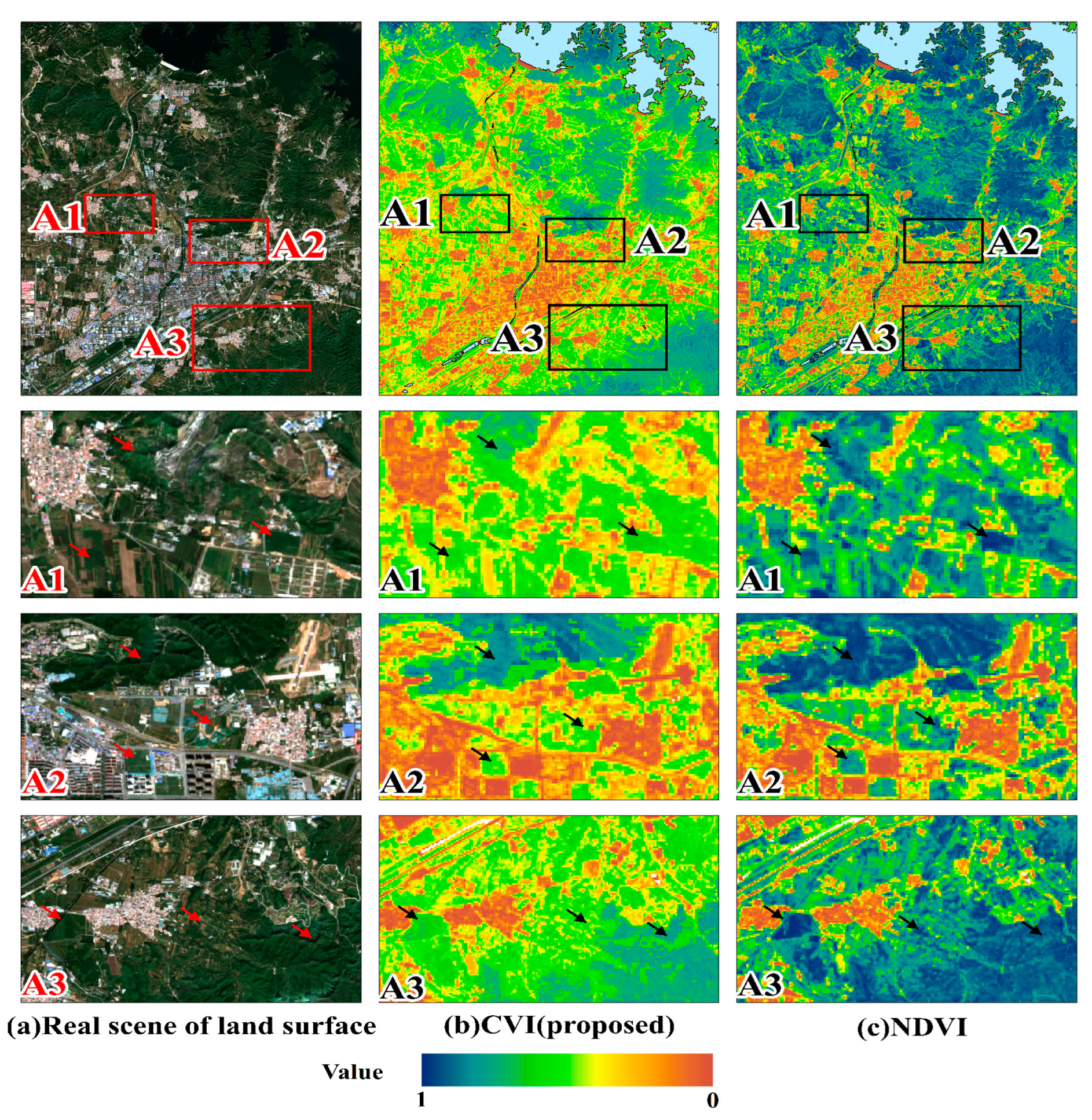
- Vegetation factor
- (2)
- Wetness factor
- (3)
- Dryness factor
- (4)
- Heat factor
- (5)
- Difference factor for air quality
3.2. Model Construction
- (1)
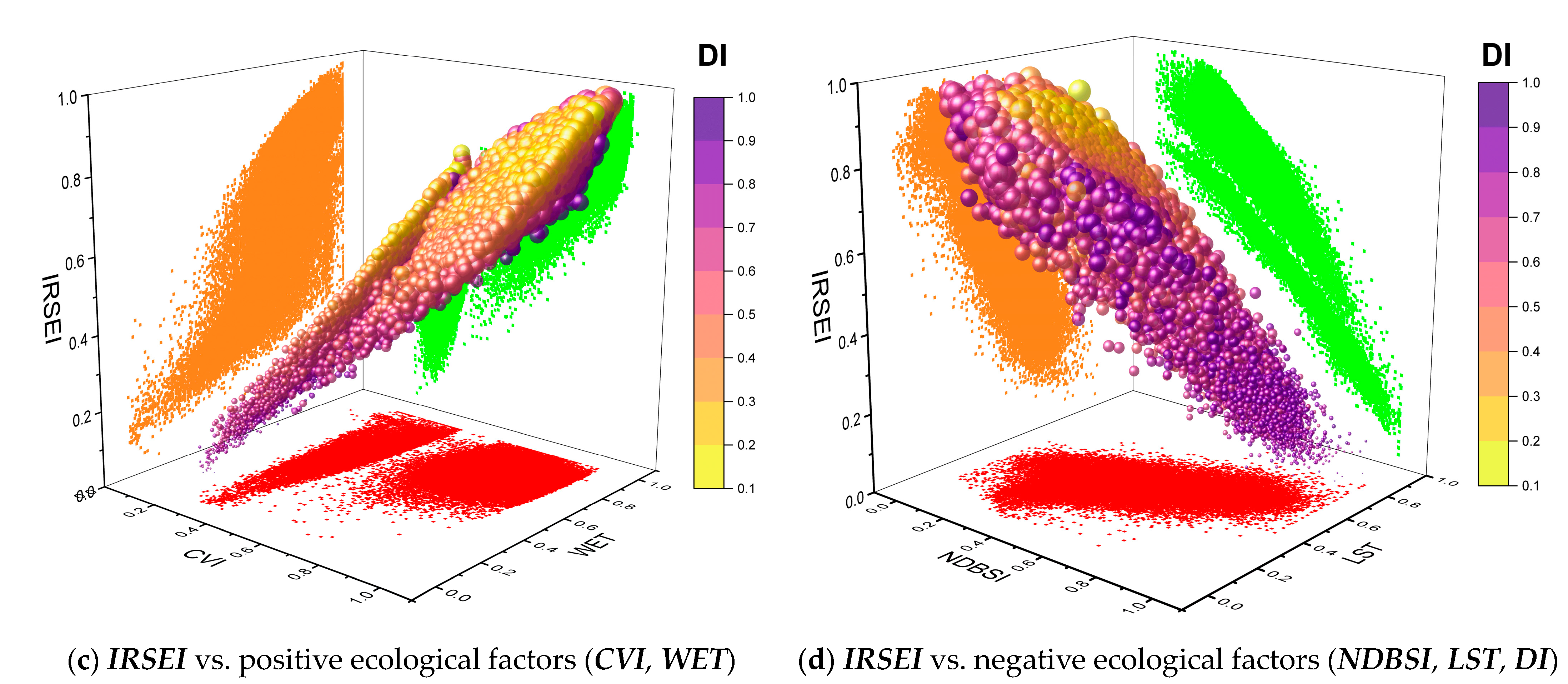
- IRSEI model
- (2)
- RSEI model
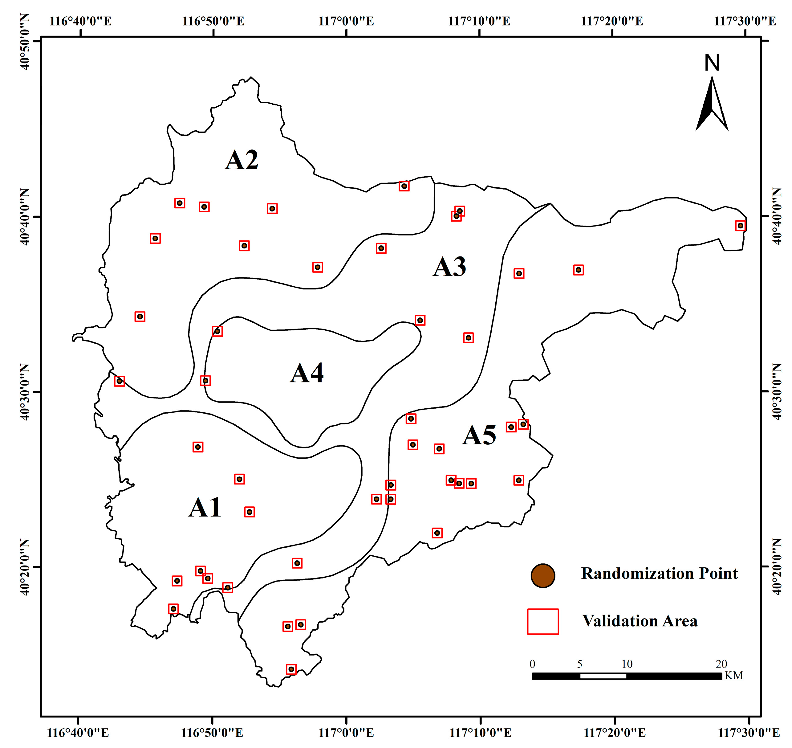
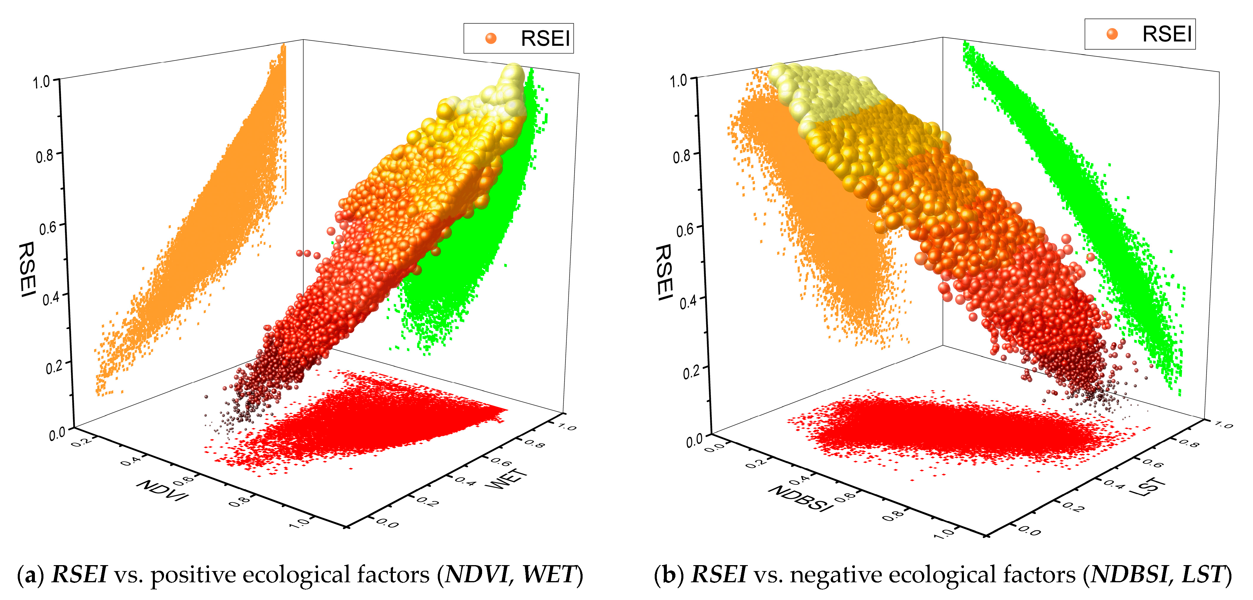
3.3. Model Validation
4. Results
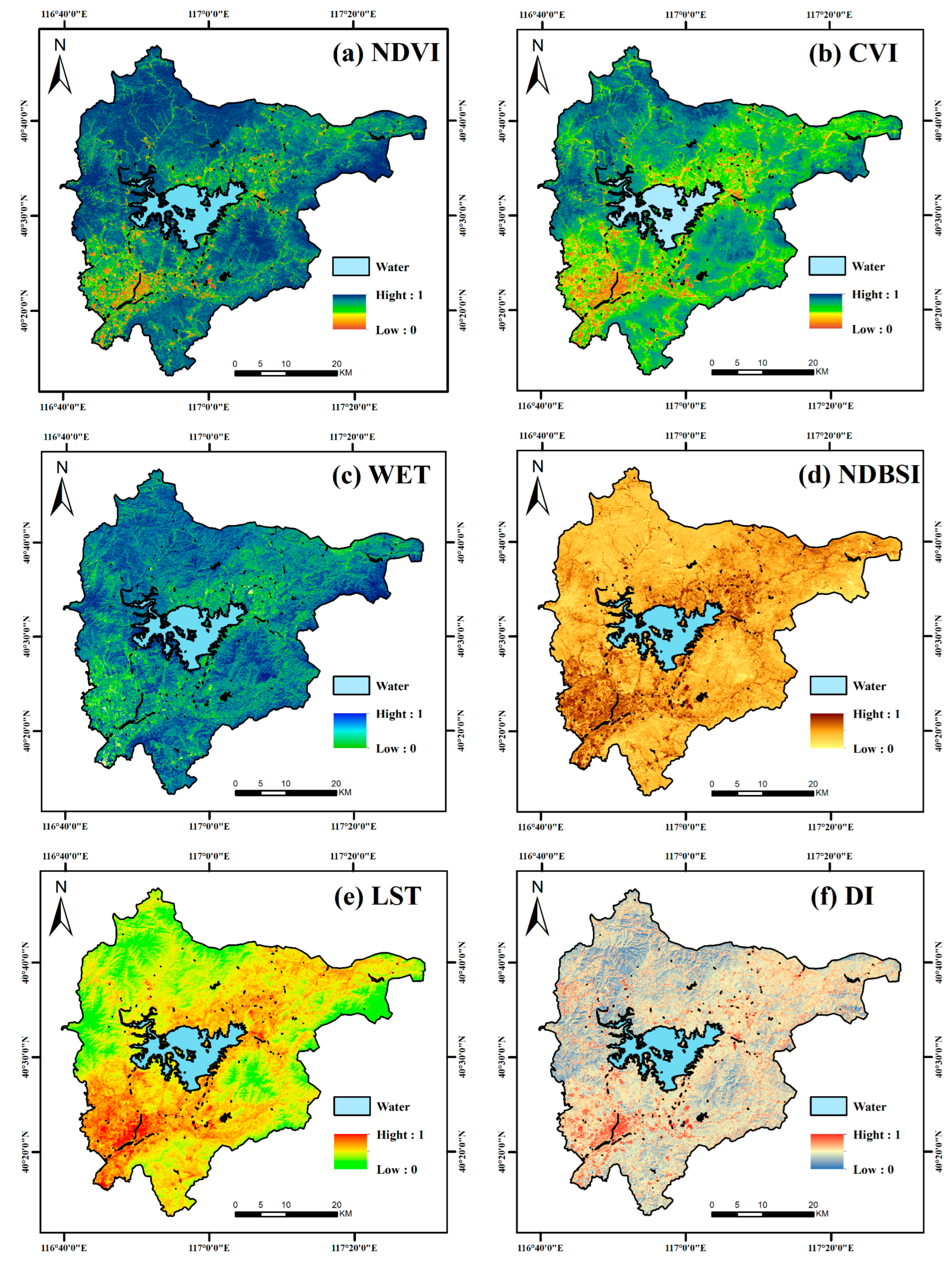
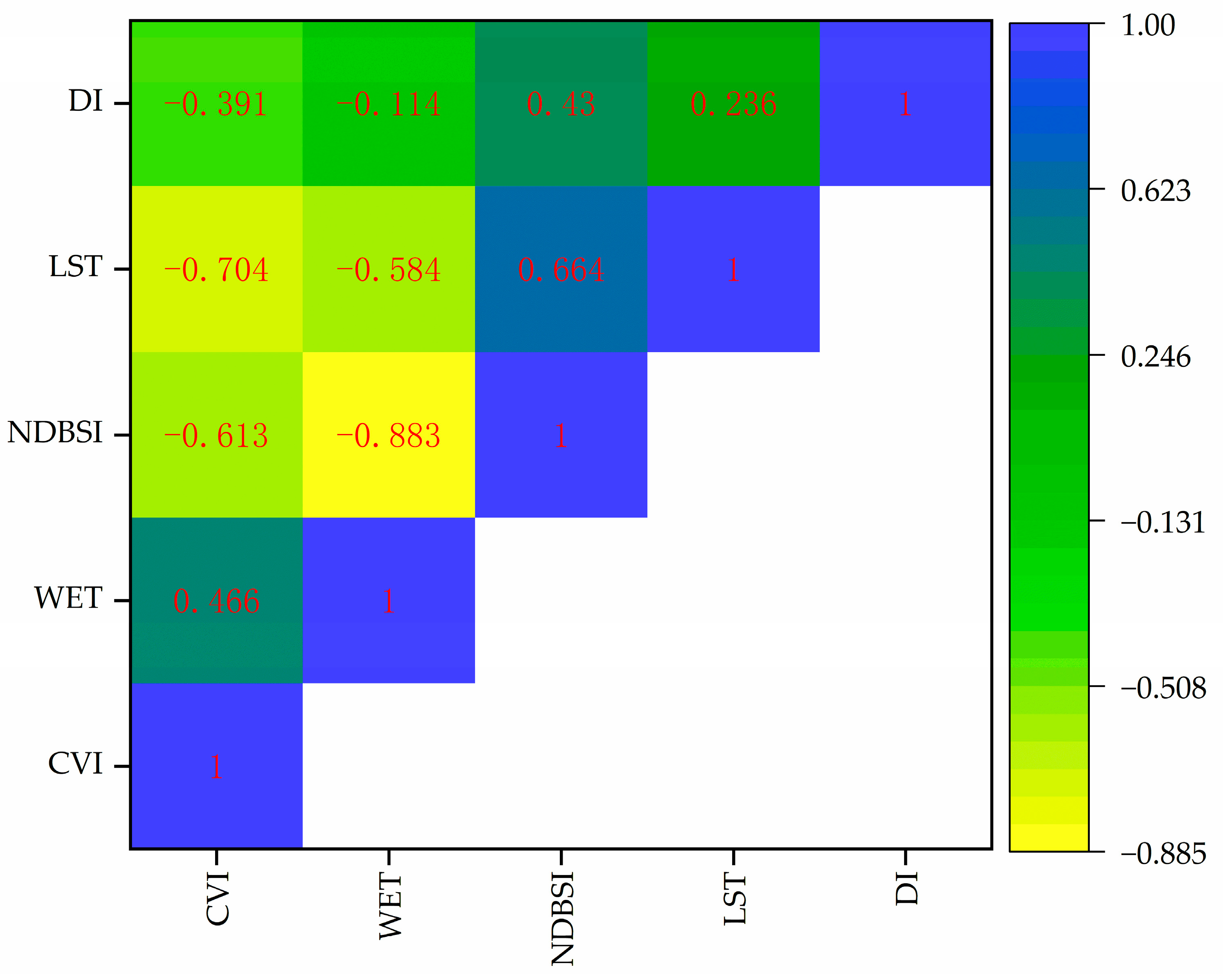
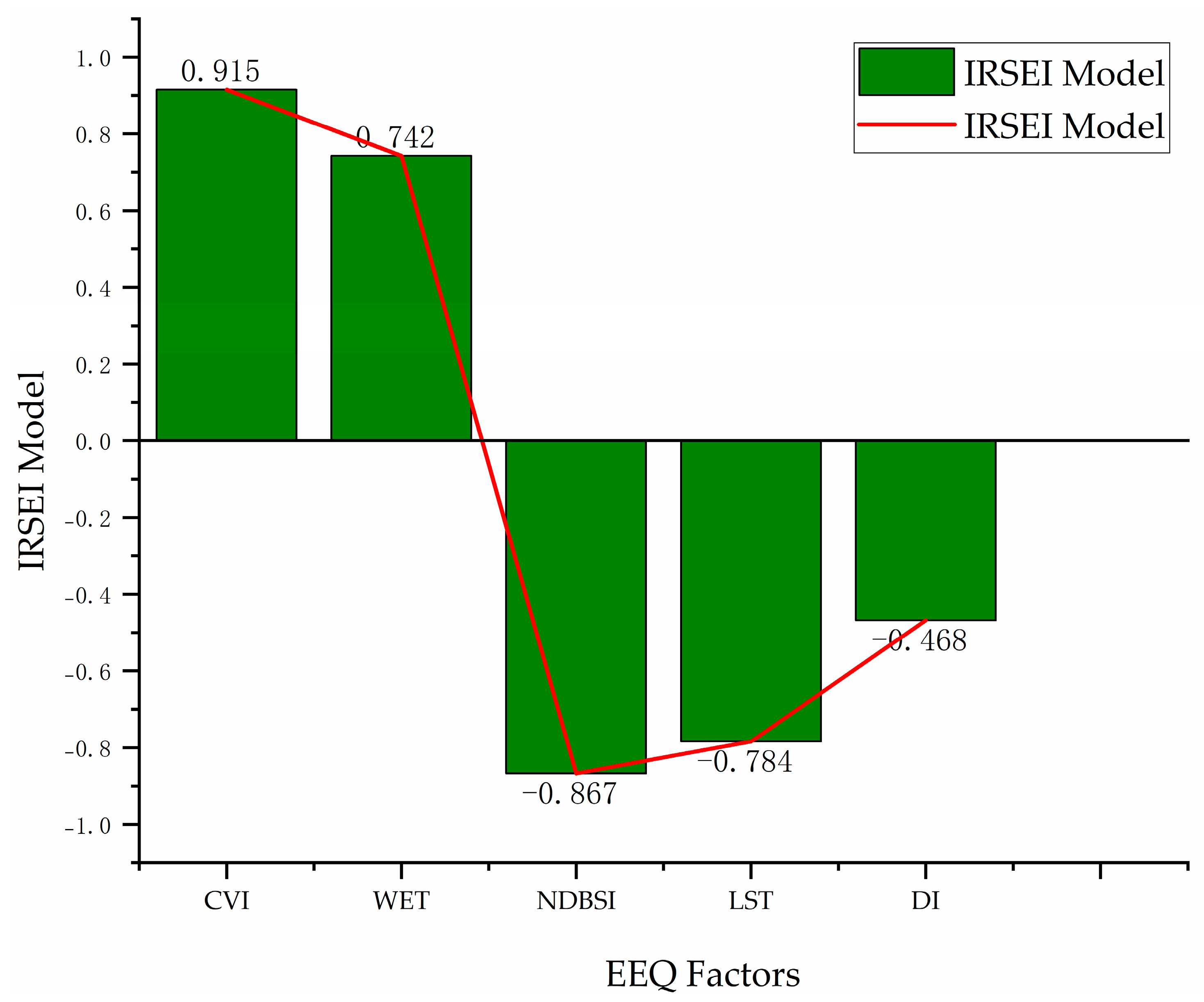
4.1. Results of Calculated Factors
4.2. Results of the Two Constructed Models
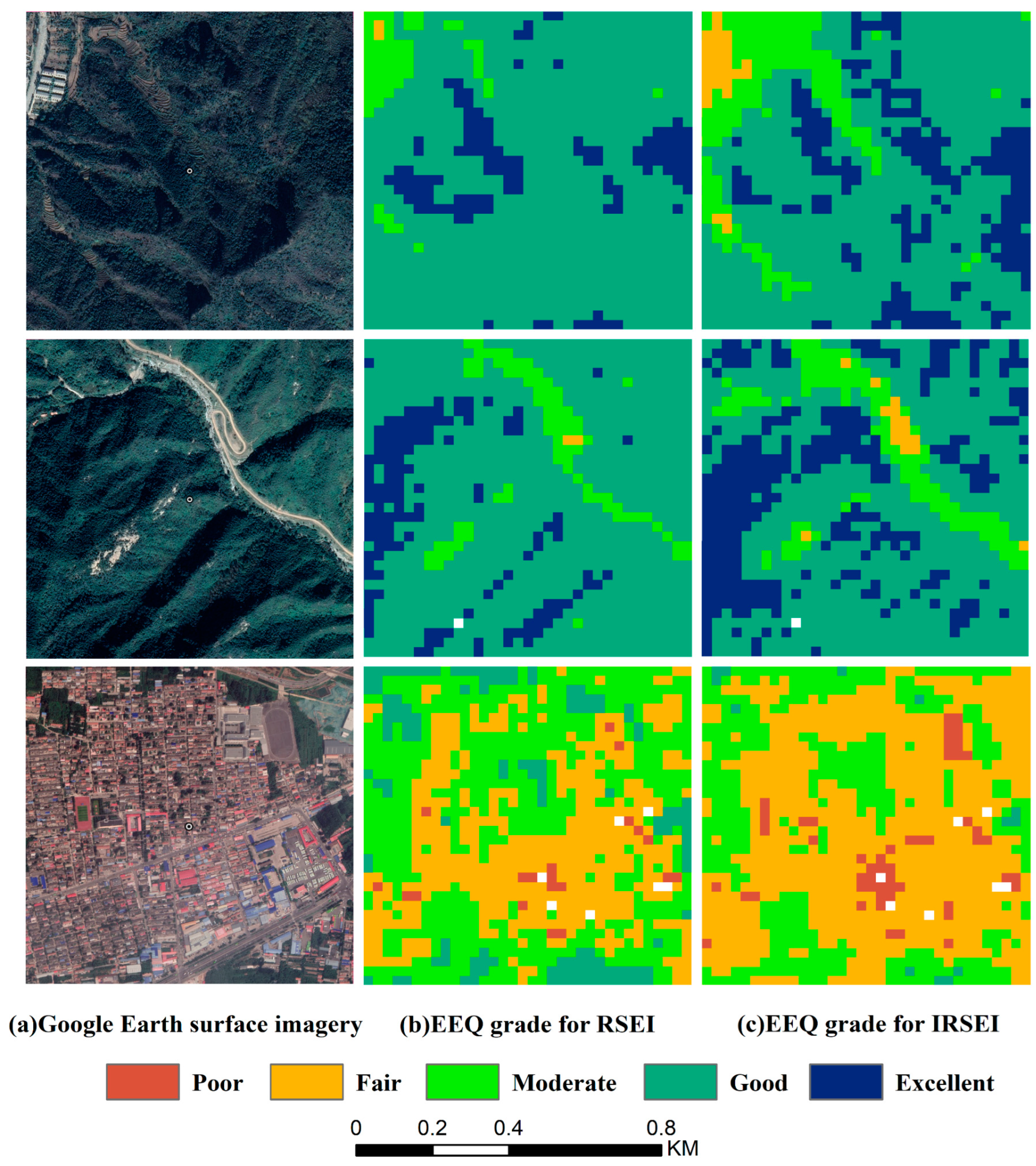
4.3. Results of Model Validation
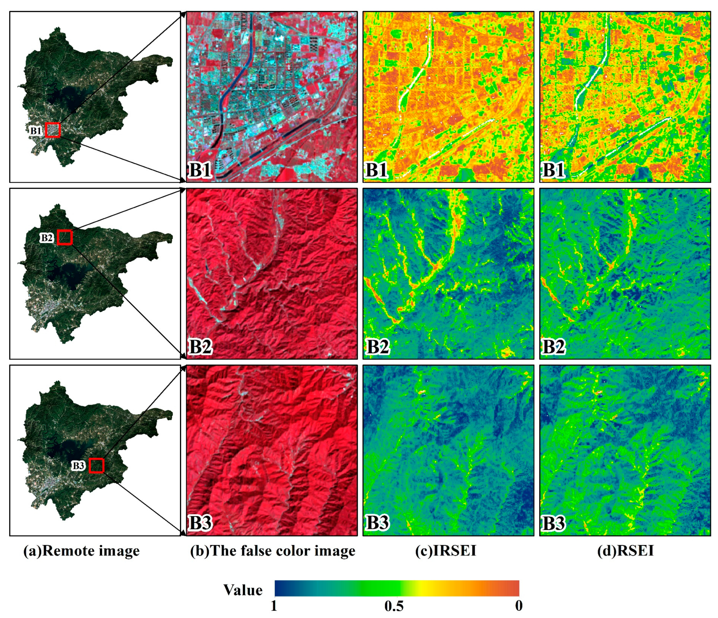
4.4. Results of Model Application in Miyun
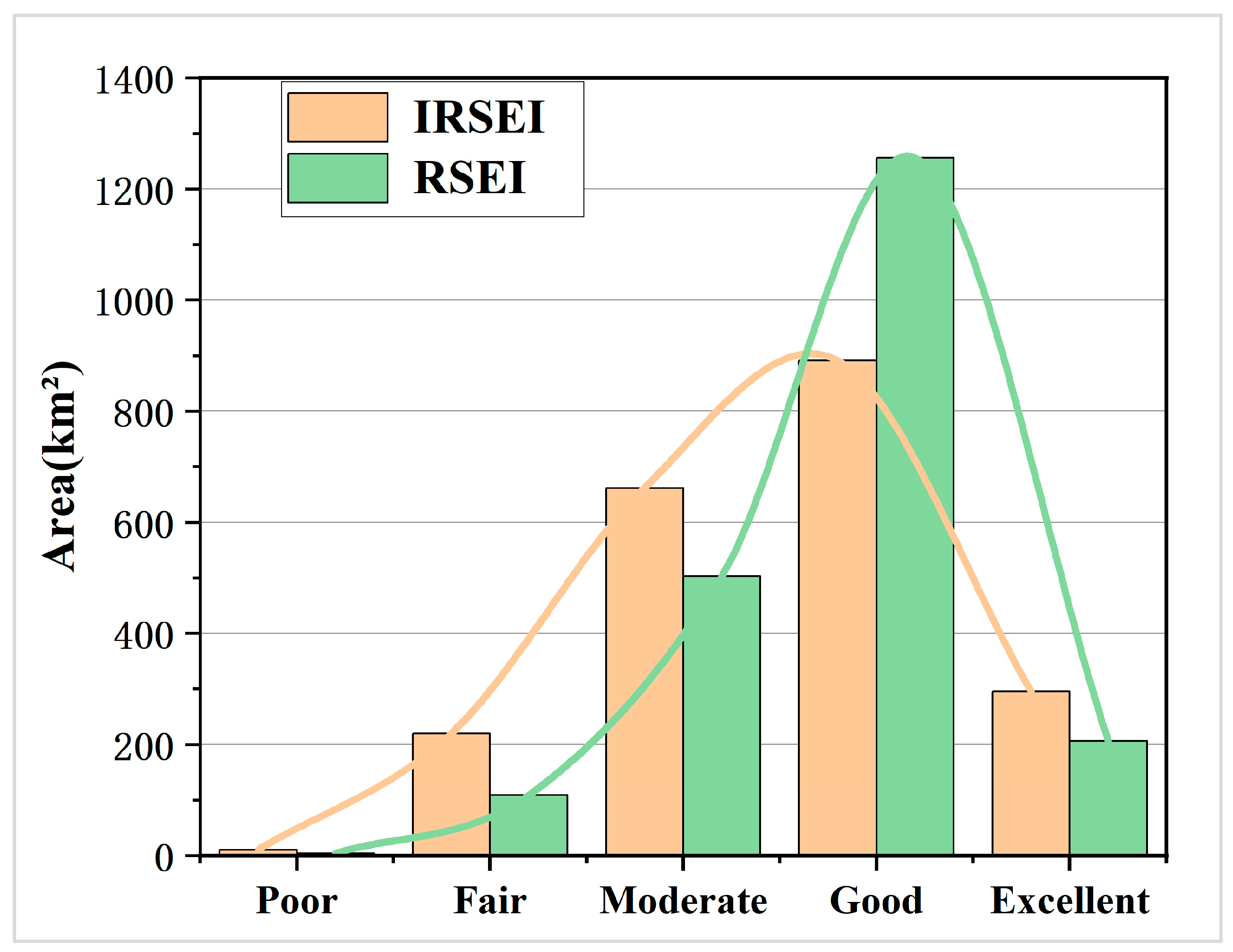
4.4.1. Evaluation of Eco-Environmental Quality (EEQ)
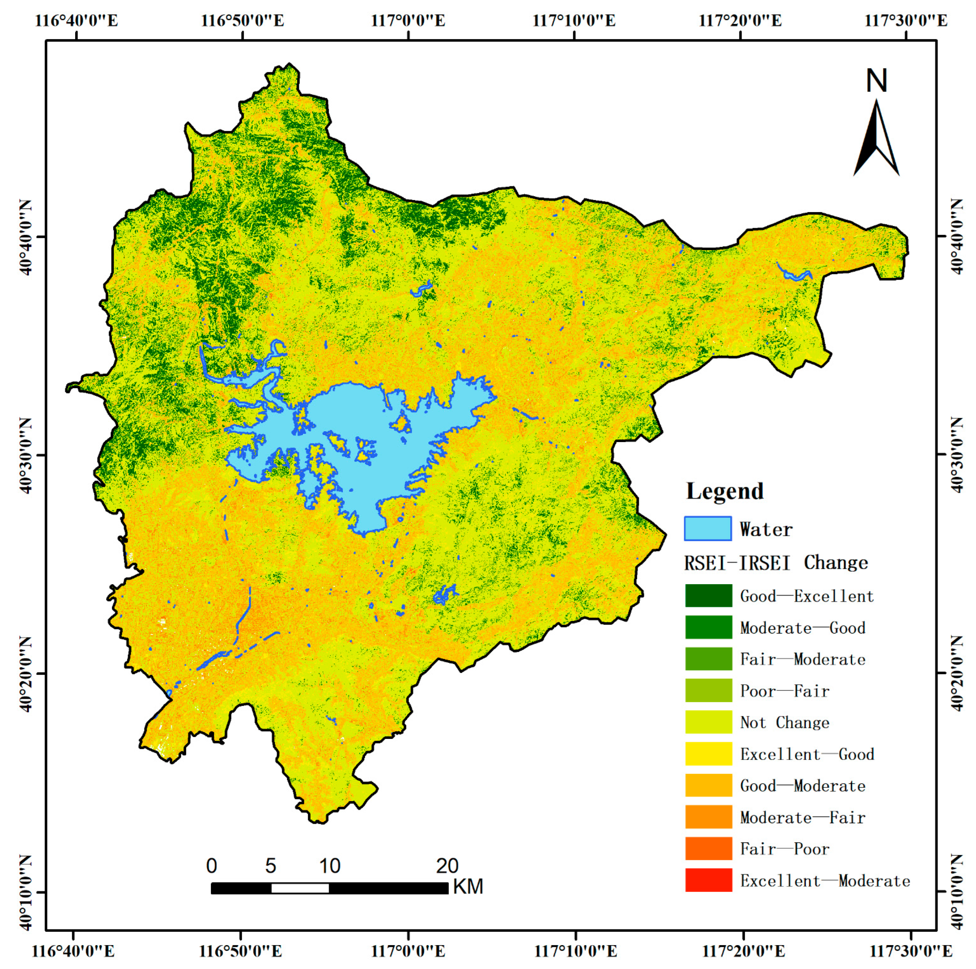
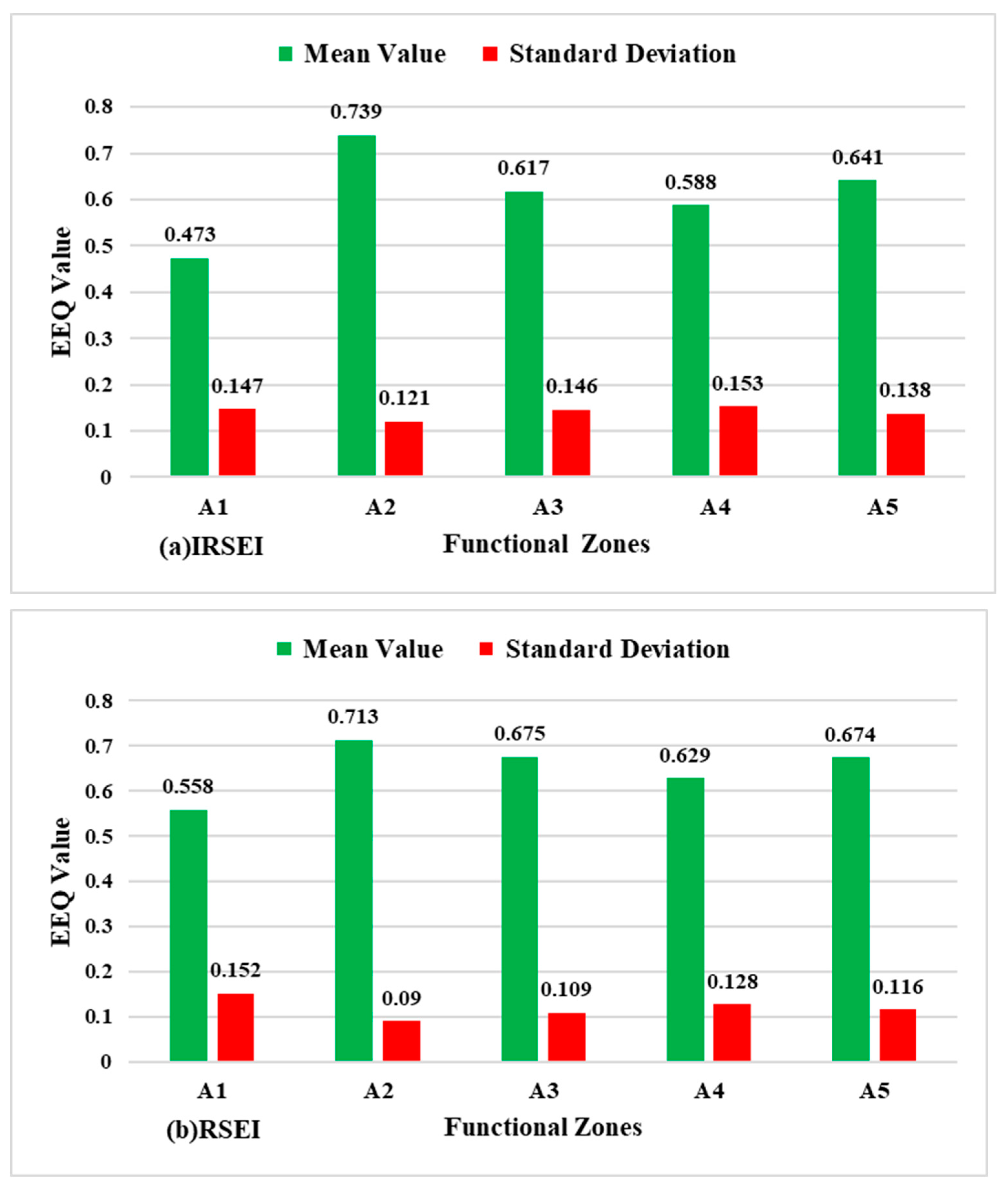
4.4.2. Consistency Assessment in Territorial Spatial Planning
5. Discussion
5.1. Advantages of 3D Factors
5.2. Comparison of RSEI and IRSEI Models
6. Conclusions
Author Contributions
Funding
Data Availability Statement
Conflicts of Interest
References
- Chen, T.; Lu, Z.Y.; Yang, Y.; Zhang, Y.X.; Du, B.; Plaza, A. A Siamese Network Based U-Net for Change Detection in High Resolution Remote Sensing Images. IEEE J. Sel. Top. Appl. Earth Obs. Remote Sens. 2022, 15, 2357–2369. [Google Scholar] [CrossRef]
- Zheng, X.X.; Chen, T. High spatial resolution remote sensing image segmentation based on the multiclassification model and the binary classification model. Neural Comput. Appl. 2023, 35, 3597–3604. [Google Scholar] [CrossRef]
- Zhang, H.; Yin, Y.X.; An, H.M.; Lei, J.P.; Li, M.; Song, J.Y.; Han, W.H. Surface urban heat island and its relationship with land cover change in five urban agglomerations in China based on GEE. Environ. Sci. Pollut. Res. 2022, 29, 82271–82285. [Google Scholar] [CrossRef] [PubMed]
- Chen, N.; Chen, Y.P.; Wang, Q.F.; Wu, S.P.; Zhang, H.Y. MAF-DeepLab: A Multiscale Attention Fusion Network for Semantic Segmentation. Trait. Du Signal 2022, 39, 407–417. [Google Scholar] [CrossRef]
- Sun, C.; Li, J.L.; Liu, Y.C.; Cao, L.D.; Zheng, J.H.; Yang, Z.J.; Ye, J.W.; Li, Y. Ecological quality assessment and monitoring using a time-series remote sensing-based ecological index (ts-RSEI). Giscience Remote Sens. 2022, 59, 1793–1816. [Google Scholar] [CrossRef]
- Tsai, Y.L.S.; Klein, I.; Dietz, A.; Oppelt, N. Monitoring Large-Scale Inland Water Dynamics by Fusing Sentinel-1 SAR and Sentinel-3 Altimetry Data and by Analyzing Causal Effects of Snowmelt. Remote Sens. 2020, 12, 3896. [Google Scholar] [CrossRef]
- Yang, C.; Cai, X.B.; Wang, X.L. Remote Sensing of Hydrological Changes in Tian-e-Zhou Oxbow Lake, an Ungauged Area of the Yangtze River Basin. Remote Sens. 2018, 10, 27. [Google Scholar] [CrossRef]
- Dallahi, Y.; Boujraf, A.; Meliho, M.; Orlando, C.A. Assessment of forest dieback on the Moroccan Central Plateau using spectral vegetation indices. J. For. Res. 2023, 34, 793–808. [Google Scholar] [CrossRef]
- Yang, Y.L.; Wang, J.L.; Chen, Y.; Cheng, F.; Liu, G.J.; He, Z.H. Remote-Sensing Monitoring of Grassland Degradation Based on the GDI in Shangri-La, China. Remote Sens. 2019, 11, 3030. [Google Scholar] [CrossRef]
- Du, Z.; Ji, X.; Liu, J.; Zhao, W.; He, Z.; Jiang, J.; Yang, Q.; Zhao, L.; Gao, J. Ecological health assessment of Tibetan alpine grasslands in Gannan using remote sensed ecological indicators. Geo-Spat. Inf. Sci. 2024, 27, 1–19. [Google Scholar] [CrossRef]
- Ning, L.; Wang, J.Y.; Fen, Q. The improvement of ecological environment index model RSEI. Arab. J. Geosci. 2020, 13, 1866–7538. [Google Scholar] [CrossRef]
- Liao, X.; Li, W.; Hou, J. Application of GIS Based Ecological Vulnerability Evaluation in Environmental Impact Assessment of Master Plan of Coal Mining Area. Procedia Environ. Sci. 2013, 18, 271–276. [Google Scholar] [CrossRef]
- Cheng, J.N.; Zhao, K.X.; Li, H.; Tang, X.M.; Suo, Q.K. Dynamic changes and evaluation of land ecological environment status based on RS and GIS technique. Trans. Chin. Soc. Agric. Eng. (Trans. CSAE) 2008, 24, 83–88. (In Chinese) [Google Scholar]
- Xu, S.; Bu, R.T.Y. Monitoring and evaluation of eco-environmental quality in Anhui Province in 2015 based on remote sensing. Environ. Dev. 2016, 28, 24–28. (In Chinese) [Google Scholar] [CrossRef]
- Yue, A.; Zhang, Z. Research on analyzing changes in ecological status based on EI values. J. Green Sci. Technol. 2018, 14, 182+184. [Google Scholar] [CrossRef]
- Ouyang, L.; Ma, H.Y.; Wang, Z.M.; Lu, C.Y.; Wang, C.L.; Zhang, Y.S.; Yu, X.S. Dynamic evaluation of ecological environment in Horqin sandy land based on remote sensing and geographic information data. Acta Ecol. Sin. 2022, 42, 5906–5921. [Google Scholar] [CrossRef]
- Li, Y.C.; Yuan, J.G.; Liu, B.H.; Guo, H. Ecological Environment Dynamical Evaluation of Hutuo River Basin Using Remote Sensing. Environ. Sci. 2023, 45, 1–18. [Google Scholar] [CrossRef]
- Xu, H.Q. A remote sensing index for assessment of regional ecological changes. China Environ. Sci. 2013, 33, 889–897. (In Chinese) [Google Scholar]
- Shan, W.; Jin, X.; Ren, J.; Wang, Y.; Xu, Z.; Fan, Y.; Gu, Z.; Hong, C.; Lin, J.; Zhou, Y. Ecological environment quality assessment based on remote sensing data for land consolidation. J. Clean. Prod. 2019, 239, 118126. [Google Scholar] [CrossRef]
- Hao, H.; Feifan, Y. Evaluation Of Spatial And Temporal Changes Of Mine Ecological Environment In Ili Valley Based On Remote Sensing Ecological Index. J. Environ. Prot. Ecol. 2022, 23, 2124–2132. [Google Scholar] [CrossRef]
- Liu, Q.; Yu, F.H.; Mu, X.M. Evaluation of the Ecological Environment Quality of the Kuye River Source Basin Using the Remote Sensing Ecological Index. Int. J. Environ. Res. Public Health 2022, 19, 12500. [Google Scholar] [CrossRef]
- Hu, X.S.; Xu, H.Q. A new remote sensing index for assessing the spatial heterogeneity in urban ecological quality: A case from Fuzhou City, China. Ecol. Indic. 2018, 89, 11–21. [Google Scholar] [CrossRef]
- Zhang, P.P.; Chen, X.D.; Ren, Y.; Lu, S.Q.; Song, D.W.; Wang, Y.L. A Novel Mine-Specific Eco-Environment Index (MSEEI) for Mine Ecological Environment Monitoring Using Landsat Imagery. Remote Sens. 2023, 15, 933. [Google Scholar] [CrossRef]
- Dong, C.Y.; Qiao, R.R.; Yang, Z.C.; Luo, L.H.; Chang, X.L. Eco-environmental quality assessment of the artificial oasis of Ningxia section of the Yellow River with the MRSEI approach. Front. Environ. Sci. 2023, 10, 1071631. [Google Scholar] [CrossRef]
- Zhang, W.; Du, P.J.; Guo, S.C.; Lin, C.; Zheng, H.R.; Fu, P.J. Enhanced remote sensing ecological index and ecological environment evaluation in arid area. Natl. Remote Sens. Bull. 2023, 27, 299–317. [Google Scholar] [CrossRef]
- Wang, Z.W.; Chen, T.; Zhu, D.Y.; Jia, K.; Plaza, A. RSEIFE: A new remote sensing ecological index for simulating the land surface eco-environment. J. Environ. Manag. 2023, 326, 116851. [Google Scholar] [CrossRef]
- Song, M.J.; Luo, Y.Y.; Duan, L.M. Evaluation of Ecological Environment in the Xilin Gol Steppe Based on Modified Remote Sensing Ecological Index Model. Arid. Zone Res. 2019, 36, 1521–1527. [Google Scholar] [CrossRef]
- Liu, Y.; Dang, C.Y.; Yue, H.; Lyu, C.G.; Qian, J.X.; Zhu, R. Comparison between modified remote sensing ecological index and RSEI. Natl. Remote Sens. Bull. 2022, 26, 683–697. [Google Scholar] [CrossRef]
- Yang, X.Y.; Meng, F.; Fu, P.J.; Wang, Y.Q.; Liu, Y.H. Time-frequency optimization of RSEI: A case study of Yangtze River Basin. Ecol. Indic. 2022, 141, 109080. [Google Scholar] [CrossRef]
- Zhang, Z.M.; Fan, Y.G.; Jiao, Z.J.; Fan, B.W.; Zhou, J.W.; Li, Z.H. Vegetation ecological benefits index (VEBI): A 3D spatial model for evaluating the ecological benefits of vegetation. Int. J. Digit. Earth 2023, 16, 1108–1123. [Google Scholar] [CrossRef]
- Lai, S.H.; Sha, J.M.; Eladawy, A.; Li, X.M.; Wang, J.L.; Kurbanov, E.; Lin, Z.J.; Wu, L.B.; Han, R.; Su, Y.C. Evaluation of ecological security and ecological maintenance based on pressure-state-response (PSR) model, case study: Fuzhou city, China. Hum. Ecol. Risk Assess. 2022, 28, 734–761. [Google Scholar] [CrossRef]
- Wang, Y.Q.; Wu, Z.J.; Yan, B.; Li, K.; Huang, F. Research on ecological environment impact assessment based on PSR and cloud theory in Dari county, source of the Yellow River. Water Supply 2021, 21, 1050–1060. [Google Scholar] [CrossRef]
- Zhang, H.F.; Li, S.D.; Liu, Y.; Xu, M. Assessment of the Habitat Quality of Offshore Area in Tongzhou Bay, China: Using Benthic Habitat Suitability and the InVEST Model. Water 2022, 14, 1574. [Google Scholar] [CrossRef]
- Wu, J.J.; Wang, X.; Zhong, B.; Yang, A.X.; Jue, K.S.; Wu, J.H.; Zhang, L.; Xu, W.J.; Wu, S.L.; Zhang, N.; et al. Ecological environment assessment for Greater Mekong Subregion based on Pressure-State-Response framework by remote sensing. Ecol. Indic. 2020, 117, 106521. [Google Scholar] [CrossRef]
- Men, B.H.; Liu, H.Y. Water resource system vulnerability assessment of the Heihe River Basin based on pressure-state-response (PSR) model under the changing environment. Water Sci. Technol.-Water Supply 2018, 18, 1956–1967. [Google Scholar] [CrossRef]
- He, J.H.; Huang, J.L.; Li, C. The evaluation for the impact of land use change on habitat quality: A joint contribution of cellular automata scenario simulation and habitat quality assessment model. Ecol. Model. 2017, 366, 58–67. [Google Scholar] [CrossRef]
- Yu, J.B.; Li, X.H.; Guan, X.B.; Shen, H.F. A remote sensing assessment index for urban ecological livability and its application. Geo-Spat. Inf. Sci. 2022, 27, 289–310. [Google Scholar] [CrossRef]
- Ashraf, A.; Haroon, M.A.; Ahmad, S.; Abowarda, A.S.; Wei, C.Y.; Liu, X.H. Use of remote sensing-based pressure-state-response framework for the spatial ecosystem health assessment in Langfang, China. Environ. Sci. Pollut. Res. 2023, 30, 89395–89414. [Google Scholar] [CrossRef]
- Li, X.; Liu, Z.S.; Li, S.J.; Li, Y.X. Multi-Scenario Simulation Analysis of Land Use Impacts on Habitat Quality in Tianjin Based on the PLUS Model Coupled with the InVEST Model. Sustainability 2022, 14, 6923. [Google Scholar] [CrossRef]
- Beijing Municipal Commission of Planning and Natural Resources. Available online: https://www.bjmy.gov.cn/zwgk/zfxxgk/fdzdgknr/ghxx/fzgh/201912/t20191227_129469.html (accessed on 27 December 2019).
- United States Geological Survey. Available online: https://earthexplorer.usgs.gov/ (accessed on 25 April 2019).
- Liu, X.Q.; Su, Y.J.; Hu, T.Y.; Yang, Q.L.; Liu, B.B.; Deng, Y.F.; Tang, H.; Tang, Z.Y.; Fang, J.Y.; Guo, Q.H. Neural network guided interpolation for mapping canopy height of China’s forests by integrating GEDI and ICESat-2 data. Remote Sens. Environ. 2022, 269, 112844. [Google Scholar] [CrossRef]
- Chan, A.H.Y.; Guizar-Coutino, A.; Kalamandeen, M.; Coomes, D.A. Reconstructing 34 Years of Fire History in the Wet, Subtropical Vegetation of Hong Kong Using Landsat. Remote Sens. 2023, 15, 1489. [Google Scholar] [CrossRef]
- Laborde, H.; Douzal, V.; Pina, H.A.R.; Morand, S.; Cornu, J.F. Landsat-8 cloud-free observations in wet tropical areas: A case study in South East Asia. Remote Sens. Lett. 2017, 8, 537–546. [Google Scholar] [CrossRef]
- Xu, H.Q.; Duan, W.F.; Deng, W.H.; Lin, M.J. RSEI or MRSEI? Comment on Jia et al. Evaluation of Eco-Environmental Quality in Qaidam Basin Based on the Ecological Index (MRSEI) and GEE. Remote Sens. 2022, 14, 2072–4292. [Google Scholar] [CrossRef]
- Cheng, L.L.; Wang, Z.W.; Tian, S.F.; Liu, Y.P.; Sun, M.Y.; Yang, M.Y. Evaluation of eco-environmental quality in Mentougou District of Beijing based on improved remote sensing ecological index. Chin. J. Ecol. 2021, 40, 1177–1185. [Google Scholar] [CrossRef]
- Xu, S.; Xu, D.; Liu, L. Construction of regional informatization ecological environment based on the entropy weight modified AHP hierarchy model. Sustain. Comput. Inform. Syst. 2019, 22, 26–31. [Google Scholar] [CrossRef]
- Uddin, M.P.; Al Mamun, M.A.; Hossain, M.A. PCA-based Feature Reduction for Hyperspectral Remote Sensing Image Classification. Iete Tech. Rev. 2021, 38, 377–396. [Google Scholar] [CrossRef]
- An, M.; Xie, P.; He, W.; Wang, B.; Huang, J.; Khanal, R. Spatiotemporal change of ecologic environment quality and human interaction factors in three gorges ecologic economic corridor, based on RSEI. Ecol. Indic. 2022, 141, 109090. [Google Scholar] [CrossRef]
- Yu, L.; Gong, P. Google Earth as a virtual globe tool for Earth science applications at the global scale: Progress and perspectives. Int. J. Remote Sens. 2012, 33, 3966–3986. [Google Scholar] [CrossRef]
- Yuan, Y.X.; Zhu, X.L.; Hou, C.H.; Liu, S.; Song, J.W.; Li, X.G. Spatiotemporal evolution characteristics and driving forces of surface thermal environment in mining intensive areas. Sci. Technol. Eng. 2022, 22, 14537–14548. (In Chinese) [Google Scholar]
- Kucuker, D.M.; Giraldo, D.C. Assessment of soil erosion risk using an integrated approach of GIS and Analytic Hierarchy Process (AHP) in Erzurum, Turkiye. Ecol. Inform. 2022, 71, 101788. [Google Scholar] [CrossRef]
- Gou, R.; Zhao, J. Eco-environmental quality monitoring in Beijing, China, using an RSEI-based approach combined with random forest algorithms. IEEE Access 2020, 8, 196657–196666. [Google Scholar] [CrossRef]
- Liu, Y.; Xu, W.H.; Hong, Z.H.; Wang, L.G.; Ou, G.L.; Lu, N.; Dai, Q.L. Integrating three-dimensional greenness into RSEI improved the scientificity of ecological environment quality assessment for forest. Ecol. Indic. 2023, 156, 111092. [Google Scholar] [CrossRef]
- Li, Y.; Wu, L.Y.; Han, Q.; Wang, X.; Zou, T.Q.; Fan, C. Estimation of remote sensing based ecological index along the Grand Canal based on PCA-AHP-TOPSIS methodology. Ecol. Indic. 2021, 122, 107214. [Google Scholar] [CrossRef]
- Yan, S.J.; Wang, X.; Cai, Y.P.; Li, C.H.; Yan, R.; Cui, G.N.; Yang, Z.F. An Integrated Investigation of Spatiotemporal Habitat Quality Dynamics and Driving Forces in the Upper Basin of Miyun Reservoir, North China. Sustainability 2018, 10, 4625. [Google Scholar] [CrossRef]
- Beijing Municipal Ecology and Environment Bureau. Beijing Ecology and Environment Statement 2019. Available online: https://sthjj.beijing.gov.cn/bjhrb/index/xxgk69/sthjlyzwg/1718880/1718881/1718882/index.html (accessed on 27 April 2020).
- Kumar, B.P.; Babu, K.R.; Anusha, B.N.; Rajasekhar, M. Geo-environmental monitoring and assessment of land degradation and desertification in the semi-arid regions using Landsat 8 OLI/TIRS, LST, and NDVI approach. Environ. Chall. 2022, 8, 100578. [Google Scholar] [CrossRef]
- Hu, Y.G.; Li, H.; Wu, D.; Chen, W.; Zhao, X.; Hou, M.L.; Li, A.J.; Zhu, Y.J. LAI-indicated vegetation dynamic in ecologically fragile region: A case study in the Three-North Shelter Forest program region of China. Ecol. Indic. 2021, 120, 106932. [Google Scholar] [CrossRef]
- Wang, Z.; Bai, T.; Xu, D.; Kang, J.; Shi, J.; Fang, H.; Nie, C.; Zhang, Z.; Yan, P.; Wang, D. Temporal and Spatial Changes in Vegetation Ecological Quality and Driving Mechanism in Kökyar Project Area from 2000 to 2021. Sustainability 2022, 14, 7668. [Google Scholar] [CrossRef]
- Gebremedhin, A.; Badenhorst, P.; Wang, J.; Giri, K.; Spangenberg, G.; Smith, K. Development and Validation of a Model to Combine NDVI and Plant Height for High-Throughput Phenotyping of Herbage Yield in a Perennial Ryegrass Breeding Program. Remote Sens. 2019, 11, 2494. [Google Scholar] [CrossRef]
- Zhou, L.; Ou, G.; Wang, J.; Xu, H. Light saturation point determination and biomass remote sensing estimation of Pinus kesiya var. langbianensis forest based on spatial regression models. Sci. Silvae Sin 2020, 56, 38–47. [Google Scholar] [CrossRef]
- Zhou, J.-L.; Xu, Q.-Q.; Zhang, X.-Y. Water Resources and Sustainability Assessment Based on Group AHP-PCA Method: A Case Study in the Jinsha River Basin. Water 2018, 10, 1880. [Google Scholar] [CrossRef]
- Lever, J.; Krzywinski, M.; Altman, N. Points of significance: Principal component analysis. Nat. Methods 2017, 14, 641–643. [Google Scholar] [CrossRef]
- Shan, W.; Jin, S.B.; Meng, X.S.; Yang, X.Y.; Xu, Z.G.; Gu, Z.M.; Zhou, Y.K. Dynamical monitoring of ecological environment quality of land consolidation based on multi-source remote sensing data. Trans. Chin. Soc. Agric. Eng. 2019, 35, 234–242. [Google Scholar] [CrossRef]
- Hang, X.; Luo, X.Y.; Cao, Y.; Li, Y.C. Ecological quality assessment and the impact of urbanization based on RSEI model for Nanjing, Jiangsu Province, China. Chin. J. Appl. Ecol. 2020, 31, 219–229. [Google Scholar] [CrossRef]
- Zheng, Z.C.; Chang, S.T.; Chen, W.H.; Wang, M.S.; Wu, S.J.; Chen, B.Q. Remote Sensing Monitoring and Evaluation of Ecological Environment Quality in Pingtan Comprehensive Experimental Area from 2007 to 2017. J. Fujian Norm. Univ. (Nat. Sci. Ed.) 2019, 35, 89–97. [Google Scholar] [CrossRef]
- Zheng, Z.H.; Wu, Z.F.; Chen, Y.B.; Guo, C.; Marinello, F. Instability of remote sensing based ecological index (RSEI) and its improvement for time series analysis. Sci. Total Environ. 2022, 814, 152595. [Google Scholar] [CrossRef] [PubMed]
- Xu, H.Q.; Wang, Y.F.; Guan, H.D.; Shi, T.T.; Hu, X.S. Detecting Ecological Changes with a Remote Sensing Based Ecological Index (RSEI) Produced Time Series and Change Vector Analysis. Remote Sens. 2019, 11, 2345. [Google Scholar] [CrossRef]
- Mao, X.; Wang, H. Assessing ecological and environmental vulnerability of Miyun County in Beijing according to pixel scale. J. Nanjing For. Univ. 2017, 60, 96. [Google Scholar] [CrossRef]
- Airiken, M.; Zhang, F.; Chan, N.W.; Kung, H.-t. Assessment of spatial and temporal ecological environment quality under land use change of urban agglomeration in the North Slope of Tianshan, China. Environ. Sci. Pollut. Res. 2022, 29, 12282–12299. [Google Scholar] [CrossRef]


| Grade | Values | Ecological Performance |
|---|---|---|
| Excellent | [1, 0.8) | High-vegetation cover, good natural conditions, and stable ecosystems. |
| Good | [0.8, 0.6) | Good natural conditions and good vegetation cover for human life. |
| Moderate | [0.6, 0.4) | Vegetation cover is medium and more suitable for human life. |
| Fair | [0.4, 0.2) | Vegetation cover is poor and arid and there are limiting factors for human life. |
| Poor | [0.2, 0] | Low vegetation cover, harsh conditions, and restrictions on human life |
| Model | Factors | PC1 | PC2 | PC3 | PC4 | PC5 |
|---|---|---|---|---|---|---|
| IRSEI (Proposed) | CVI | 0.703 | 0.609 | 0.257 | 0.260 | 0.019 |
| WET | 0.382 | −0.616 | 0.152 | 0.212 | 0.638 | |
| NDBSI | −0.491 | 0.463 | 0.235 | −0.041 | 0.698 | |
| LST | −0.288 | 0.005 | −0.165 | 0.938 | −0.096 | |
| DI | −0.188 | −0.188 | 0.910 | 0.071 | −0.310 | |
| EV 1 | 0.032 | 0.008 | 0.005 | 0.002 | 0 | |
| pEV (%) 2 | 68.169 | 17.266 | 10.257 | 3.286 | 1.023 | |
| RSEI (Original) | NDVI | 0.337 | −0.384 | 0.550 | 0.661 | |
| WET | 0.572 | 0.575 | −0.429 | 0.399 | ||
| NDBSI | −0.671 | −0.057 | −0.385 | 0.630 | ||
| LST | −0.330 | 0.721 | 0.604 | 0.083 | ||
| EV 1 | 0.021 | 0.002 | 0.001 | 0 | ||
| pEV (%) 2 | 83.25 | 9.56 | 6.00 | 1.150 |
| Ecological Factors | Weight | CI | RI | CR | |||||
|---|---|---|---|---|---|---|---|---|---|
| CVI | WET | NDBSI | LST | DI | |||||
| CVI | 1 | 3 | 2 | 4 | 3 | 0.398 | 0.023 | 1.12 | 0.021 |
| WET | 1/3 | 1 | 1/2 | 2 | 2 | 0.160 | |||
| NDBSI | 1/2 | 2 | 1 | 3 | 2 | 0.242 | |||
| LST | 1/4 | 1/2 | 1/3 | 1 | 1/2 | 0.079 | |||
| DI | 1/3 | 1/2 | 1/2 | 2 | 1 | 0.122 | |||
| Factors | CVI | WET | NDBSI | LST | DI |
|---|---|---|---|---|---|
| Weights (Wi) | 0.372 | 0.173 | 0.242 | 0.107 | 0.106 |
| Model | The Number of EEQ Grades That Matched the Reference Grades | Overall Accuracy (OA) |
|---|---|---|
| RSEI | 34/44 | 77.27% |
| IRSEI | 37/44 | 84.09% |
| EEQ Grade | IRSEI | |||||
|---|---|---|---|---|---|---|
| Poor | Fair | Moderate | Good | Excellent | ||
| R S E I | Poor | 4.41 | 0.076 | |||
| Fair | 6.271 | 98.748 | 3.311 | |||
| Moderate | 121.076 | 319.154 | 63.118 | |||
| Good | 338.877 | 754.036 | 162.845 | |||
| Excellent | 0.157 | 73.867 | 132.396 | |||
| Zones | Models | Poor | Fair | Moderate | Good | Excellent |
|---|---|---|---|---|---|---|
| A1 | IRSEI | 6.651 | 113.56 | 171.783 | 69.435 | 3.071 |
| RSEI | 2.941 | 59.13 | 145.638 | 142.868 | 13.924 | |
| A2 | IRSEI | 0.345 | 10.203 | 61.789 | 264.264 | 185.36 |
| RSEI | 0.147 | 4.921 | 48.485 | 394.54 | 73.868 | |
| A3 | IRSEI | 0.059 | 3.852 | 26.536 | 26.337 | 6.107 |
| RSEI | 0.024 | 0.964 | 13.511 | 41.489 | 6.899 | |
| A4 | IRSEI | 2.624 | 65.119 | 203.305 | 240.184 | 32.975 |
| RSEI | 1.061 | 31.507 | 160.15 | 316.071 | 35.422 | |
| A5 | IRSEI | 0.695 | 25.348 | 196.223 | 288.886 | 72.348 |
| RSEI | 0.23 | 10.706 | 131.989 | 360.203 | 80.373 |
Disclaimer/Publisher’s Note: The statements, opinions and data contained in all publications are solely those of the individual author(s) and contributor(s) and not of MDPI and/or the editor(s). MDPI and/or the editor(s) disclaim responsibility for any injury to people or property resulting from any ideas, methods, instructions or products referred to in the content. |
© 2024 by the authors. Licensee MDPI, Basel, Switzerland. This article is an open access article distributed under the terms and conditions of the Creative Commons Attribution (CC BY) license (https://creativecommons.org/licenses/by/4.0/).
Share and Cite
Liu, Y.; Xiang, W.; Hu, P.; Gao, P.; Zhang, A. Evaluation of Ecological Environment Quality Using an Improved Remote Sensing Ecological Index Model. Remote Sens. 2024, 16, 3485. https://doi.org/10.3390/rs16183485
Liu Y, Xiang W, Hu P, Gao P, Zhang A. Evaluation of Ecological Environment Quality Using an Improved Remote Sensing Ecological Index Model. Remote Sensing. 2024; 16(18):3485. https://doi.org/10.3390/rs16183485
Chicago/Turabian StyleLiu, Yanan, Wanlin Xiang, Pingbo Hu, Peng Gao, and Ai Zhang. 2024. "Evaluation of Ecological Environment Quality Using an Improved Remote Sensing Ecological Index Model" Remote Sensing 16, no. 18: 3485. https://doi.org/10.3390/rs16183485