Investigation and Validation of Split-Window Algorithms for Estimating Land Surface Temperature from Landsat 9 TIRS-2 Data

Abstract

Land surface temperature (LST) is important in a variety of applications, such as urban thermal environment monitoring and water resource management. In this paper, eleven candidate split-window (SW) algorithms were adapted to Thermal Infrared Sensor-2 (TIRS-2) data of the Landsat 9 satellite for estimating the LST. The simulated dataset produced by extensive radiative transfer modeling and five global atmospheric profile databases was used to determine the SW algorithm coefficients. Ground measurements gathered at Surface Radiation Budget Network sites were used to confirm the efficiency of the SW algorithms after their performance was initially examined using the independent simulation dataset. Five atmospheric profile databases perform similarly in training accuracy under various subranges of total water vapor. The candidate SW algorithms demonstrate superior performance compared to the radiative transfer equation algorithm, exhibiting a reduction in overall bias and RMSE by 1.30 K and 1.0 K, respectively. It is expected to provide guidance for the generation of the Landsat 9 LST using the SW algorithms.

1. Introduction

Land surface temperature and emissivity (LST&E) are the key parameters to control the water and energy budget balance and have been identified as important Earth System Data Records (ESDRs) by the National Aeronautics and Space Administration (NASA) and many other international organizations [1,2,3,4,5]. The LST product generated from thermal infrared (TIR) remote sensing provides a unique opportunity to obtain the LST at regional and global scales and has been widely used in hydrology, meteorology, and surface energy balance [6,7,8].

With the launch of Landsat 9 on 27 September 2021, the Landsat series of satellites have been providing TIR observations for 40 years, thus constituting a highly valuable data resource for the generation of LST records [9,10,11]. The integration of the Landsat 9 and Landsat 8 satellites will facilitate cooperative observations with an eight-day revisit period. Landsat 9 is equipped with the TIR Sensor-2 (TIRS-2), which features two TIR channels similar to the TIRS on Landsat 8. However, the TIRS-2 has significantly reduced stray light, thereby enabling more accurate LST [12,13]. Researchers have studied the accuracy of Landsat 9 LST products produced by the radiative transfer equation (RTE) algorithm since the United States Geological Survey (USGS) made these products available. In comparison to ground measurements, the average bias and root mean square error (RMSE) were found to be 0.24 K and 3.42 K, respectively. Additionally, the Landsat 9 LST product showed good agreement with the Landsat 7/8 LSTs [10]. The ground campaign conducted by the Rochester Institute of Technology (RIT) also indicated that Landsat 9 is exhibiting consistent behavior with Landsat 8, the ground reference, and unmanned aircraft system (UAS) measurements [9]. It should be noted that the LST differences between Landsat 8 and Landsat 9 are typically more pronounced in barren desert regions and areas with a high concentration of built-up land [14].

Since 1 March 2023, the Landsat 9 Collection 2 data from the first year of operation have been reprocessed to incorporate calibration updates identified by the USGS/NASA calibration and validation team. Using accurate ground measurements as a reference, Niclòs et al. performed vicarious calibrations on the originally calibrated and reprocessed Landsat 9 TIRS-2 data and assessed the impact of the reprocessing on the LST retrieval [15]. No significant calibration errors were observed, and both single-channel and split-window (SW) algorithms can provide LST with uncertainties around 1 K. Theoretically, the split-window algorithm performs better than the single-channel algorithm over global conditions without needing high-precision atmospheric profiles [16,17,18]. The researchers also developed SW and ensemble learning algorithms for Landsat 9 LST retrieval [11,19,20]. For example, a radiance-based split-window (RBSW) algorithm was proposed to retrieve Landsat 9 LST and the validation result indicated that a reduction of about 0.8 K in RMSE was achieved compared to the official LST product [11]. Taking full advantage of the ensemble learning method, a new algorithm is proposed to retrieve LST directly from the Landsat 9 top-of-atmosphere brightness temperature without requiring external parameters [20]. Compared to ground measurements, the algorithm achieves a bias and RMSE of −0.465 K and 2.508 K, respectively.

Over the past 30 years, various SW algorithms have been developed to perform LST retrieval using different TIR sensors. Among the published SW algorithms, which one is the most reliable and accurate is unclear because every sensor has a different filter response and central wavelength. Extensive investigations are needed to validate the accuracy of Landsat 9 LSTs derived from various SW algorithms. In this paper, we adapted eleven published SW algorithms to TIRS-2 data and evaluated their performance using ground measurements. This paper has the following structure. In Section 2, we describe the SW algorithms, the land surface emissivity estimation, the simulation dataset, and the ground LST estimation. The results and analysis are presented in Section 3. The discussion and conclusions are given in Section 4 and Section 5.

2. Datasets and Methods

2.1. Split-Window LST Algorithms

After conducting a comprehensive review of LST algorithms, we selected eleven SW algorithms from the literature as candidate algorithms for the TIRS-2, which were also summarized in previous research [21,22,23].

Table 1. Summary of the eleven candidate LST algorithms used, including names, formulas, and references.

Name	Formula	References
SW 1	$T_s=C_0+(C_1+C_2{\displaystyle \frac{1-\epsilon }{\epsilon }}+C_3{\displaystyle \frac{∆\epsilon }{{\epsilon }^2}}){\displaystyle \frac{T_{10}+T_{11}}{2}}+(C_4+C_5{\displaystyle \frac{1-\epsilon }{\epsilon }}+C_6{\displaystyle \frac{∆\epsilon }{{\epsilon }^2}}){\displaystyle \frac{T_{10}-T_{11}}{2}}$	[7,26]
SW 2	$T_s=C_0+\left(C_1+C_2{\displaystyle \frac{1-\epsilon }{\epsilon }}+C_3{\displaystyle \frac{∆\epsilon }{{\epsilon }^2}}\right){\displaystyle \frac{T_{10}+T_{11}}{2}}+\left(C_4+C_5{\displaystyle \frac{1-\epsilon }{\epsilon }}+C_6{\displaystyle \frac{∆\epsilon }{{\epsilon }^2}}\right){\displaystyle \frac{T_{10}-T_{11}}{2}}+C_7{(T_{10}-T_{11})}^2$	[27]
SW 3	$T_s=C_0+C_1{T}_{10}+C_2\left(T_{10}-T_{11}\right)+C_3{{\epsilon }_{10}T}_{10}+C_4(1-{\epsilon }_{10})\left(T_{10}-T_{11}\right)+C_5{T}_{11}∆\epsilon$	[28]
SW 4	$T_s=C_0+C_1{T}_{10}+C_2\left(T_{10}-T_{11}\right)+C_3\epsilon +C_4\epsilon \left(T_{10}-T_{11}\right)+C_5∆\epsilon$	[29]
SW 5	$T_s=C_0+C_1{\displaystyle \frac{T_{10}}{\epsilon }}+C_2{\displaystyle \frac{T_{11}}{\epsilon }}+C_3{\displaystyle \frac{1-\epsilon }{\epsilon }}$	[30]
SW 6	$T_s=C_0+C_1{T}_{10}+C_2\left(T_{10}-T_{11}\right)+C_3(1-\epsilon )+C_4∆\epsilon$	[31]
SW 7	$T_s=C_0+C_1{T}_{10}+C_2\left(T_{10}-T_{11}\right)+C_3{\displaystyle \frac{1-\epsilon }{\epsilon }}+C_4{\displaystyle \frac{∆\epsilon }{{\epsilon }^2}}$	[32]
SW 8	$T_s=C_0+C_1{T}_{10}+C_2\left(T_{10}-T_{11}\right)+C_3\epsilon$	[33]
SW 9	$T_s=C_0+C_1{T}_{10}+C_2\left(T_{10}-T_{11}\right)+C_3\epsilon +C_4{\displaystyle \frac{∆\epsilon }{\epsilon }}$	[34]
SW 10	$T_s=C_0+C_1{T}_{10}+C_2\left(T_{10}-T_{11}\right)+C_3(1-{\epsilon }_{10})+C_4∆\epsilon$	[35]
SW 11	$T_s=C_0+C_1{T}_{10}+C_2\left(T_{10}-T_{11}\right)+C_3{(T_{10}-T_{11})}^2+C_4(1-{\epsilon }_{10})+C_5∆\epsilon$	[36]

Note: $C_0-C_7$ are the split-window algorithm coefficients; $T_{10}$ and $T_{11}$ are the brightness temperatures of channels 10 and 11, respectively; $\epsilon =0.5*({\epsilon }_{10}+{\epsilon }_{11})$, $∆\epsilon ={\epsilon }_{10}-{\epsilon }_{11}$, ${\epsilon }_{10}$, and ${\epsilon }_{11}$ are the emissivity values of channels 10 and 11, respectively.

presents the formulas for the eleven candidate LST algorithms, which utilize the land surface emissivity and the brightness temperatures of two TIRS-2 bands centered at 11 and 12 μm, respectively. Although the total water vapor (TWV) can be explicitly considered in the SW algorithm, it is not considered here. On the one hand, the uncertainty in the TWV will affect the accuracy of the retrieved LST. On the other hand, previous research suggested that this led to only minor enhancements in the accuracy of SW algorithms [15,24]. Additionally, the TIRS-2 has a near-zero view zenith angle, so the path length correction term is not necessary for the SW algorithms [25].

In this study, we utilized both Landsat 9 Collection 2 (C2) Level-1 (L1) and Level-2 (L2) products obtained from https://earthexplorer.usgs.gov (accessed on 1 June 2024) for LST retrieval. The brightness temperatures of channels 10 and 11 were calculated from digital numbers provided in the Landsat 9 C2 L1 product. The Normalized Difference Vegetation Index (NDVI) was calculated using the land surface reflectance (LSR) product included in the Landsat 9 C2 L2 product. To eliminate the impact of clouds and cloud shadows, the quality assessment (QA) band was employed.

2.2. Land Surface Emissivity Estimation

Taking into account the emissivity increment from the cavity effect caused by the multiple scattering in the pixel, the Landsat 9 LSE can be calculated from the improved NDVI threshold method, which can be expressed by the following equation [37,38,39]:

$${\epsilon }_i=\left\{\begin{array}{ll}{a}_{1i}+{\displaystyle \sum _{j=2}^7}{a}_{ji}{\rho }_j& NDVI<{NDVI}_s\\ {\epsilon }_{vi}{P}_v+{\epsilon }_{si}\left(1-P_v\right)+4d\epsilon P_v\left(1-P_v\right)& {NDVI}_s\le NDVI\end{array}\right.$$

(1)

$$P_v={\left({\displaystyle \frac{NDVI-{NDVI}_s}{{NDVI}_v-{NDVI}_s}}\right)}^2$$

(2)

$$d\epsilon ={\epsilon }_{vi}(-0.435{\epsilon }_{si}+0.4343)/0.985$$

(3)

where ${\epsilon }_i$ is the Landsat LSE of channel 10 or 11,${\epsilon }_{vi}$ and ${\epsilon }_{si}$ are the vegetation and soil component emissivities, and ${\rho }_j$ is the LSR of the Operational Land Imager 2(OLI-2) channel j. According to the Advanced Spaceborne Thermal Emission and Reflection Radiometer (ASTER) spectral library,${\epsilon }_{vi}$ and ${\epsilon }_{si}$ are set to 0.9847 and 0.9706, 0.9854 and 0.9769 for channels 10 and 11, respectively. The coefficients $a_{ji}$ used to calculate the soil emissivity for Landsat 9 channels 10 and 11 are shown in

Table 2. The regression coefficients for the emissivity calculation.

Channel	a1	a2	a3	a4	a5	a6	a7
10	0.9766	−0.1068	0.1524	−0.0398	−0.0568	0.0791	−0.0712
11	0.9820	0.0265	−0.0565	0.0574	−0.0663	0.0761	−0.0603

, with corresponding root mean square errors (RMSEs) of 0.0043 and 0.0029 for channels 10 and 11, respectively.

2.3. Simulation Dataset

We utilized the moderate spectral resolution atmospheric transmittance model version 5.2 (MODTRAN5.2), global atmospheric profiles, and the ASTER/MODIS spectral library to build a comprehensive simulation database for deriving coefficients essential for the mentioned SW algorithms. The specific process was as follows:

1:

Global atmospheric profiles and the spectral response functions of TIRS-2 channels were input into the MODTRAN5.2 to obtain three atmospheric parameters (atmospheric upward radiance $L_i^{\uparrow }$, downward radiance $L_i^{\downarrow }$, and transmittance ${\tau }_i$) for TIRS-2 channels [40,41]. In previous research, the global atmospheric profile databases such as Thermodynamic Initial Guess Retrieval (TIGR) [42], Global Atmospheric Profiles from Reanalysis Information (GAPRI) [43], SeeBor V5.0 training database of global profiles (SeeBor for simplicity as follows) [44], and Cloudless Land Atmosphere Radiosounding (CLAR) [45] were frequently utilized to compute the SW algorithm coefficients for thermal sensors onboard different satellites [46,47,48,49,50,51,52]. Recently, the comprehensive clear-sky database based on the European Centre for Medium-Range Forecast (ECMWF) version-5 reanalysis (ERA5 for simplicity as follows) [53] was also used to calculate atmospheric parameters [54]. This research utilized the five atmospheric profile databases mentioned above to calculate the SW algorithm coefficients. Additionally, the radiosounding profiles collected from global radiosonde stations [40,55] were used independently for validation purposes.

2:

Emissivity spectra selected from the ASTER/MODIS spectral library were convolved with the spectral response function of TIRS-2 channels to obtain the channel-integrated LSE (${\epsilon }_i$). In total, 110 emissivity spectra were selected for simulation, including 19 vegetation types, 39 soil types, 5 snow/water types, 35 rock types, and 12 manmade material types [24].

$${\epsilon }_i={\displaystyle \frac{{\int }_{\lambda 1}^{\lambda 2}\epsilon \left(\lambda \right)f_i\left(\lambda \right)d\lambda }{{\int }_{\lambda 1}^{\lambda 2}{f}_i\left(\lambda \right)d\lambda }}$$

(4)

where ${\epsilon }_i$ is the channel-integrated LSE of channel i, $\epsilon \left(\lambda \right)$ is the measured emissivity spectra of various types, and $f_i\left(\lambda \right)$ is the spectral response function of TIRS-2 channel i.

3:

The top-of-atmosphere radiation observed by TIRS-2 channels ($L_i^{TOA}$) can be calculated from the following radiative transfer equation:

$$L_i^{TOA}={\tau }_i\left({\epsilon }_i{B}_i\left(T_s\right)+(1-{\epsilon }_i)L_i^{\downarrow }\right)+L_i^{\uparrow }$$

(5)

where $L_i^{\uparrow },L_i^{\downarrow },{\mathrm{a}\mathrm{n}\mathrm{d}\tau }_i$ are the atmospheric upward radiance, downward radiance, and transmittance of channel i, respectively. $B_i$ is the channel-averaged Planck’s radiance function of channel i. $T_s$ is the LST used for the simulation. We followed the method described in [16] and set the $T_s$ as $T_0$ − 5, $T_0$, $T_0$ + 5, $T_0$ + 10, $T_0$ + 15, and $T_0$ + 20, with $T_0$ representing the air temperature at the first layer of the atmospheric profiles [56].

4:

The brightness temperatures of TIRS-2 channels ($T_i$) can be calculated using the inversion of the Plank function [57]:

$$T_i={\displaystyle \frac{hc}{k{\lambda }_i}}{\displaystyle \frac{1}{\ln (2h{c}^2{\lambda }_i^{-5}/L_i^{TOA}+1)}}$$

(6)

where $h,c,\mathrm{a}\mathrm{n}\mathrm{d}k$ are Plank’s constant, the light speed, and Boltzmann’s constant, respectively. ${\lambda }_i$ is the central wavelength of channel i. For the TIRS-2 channels, the values are 10.8 and 12.0 $\mu m$, respectively [58].

5:

The SW algorithm coefficients in Table 1 are determined by ordinary least squares linear regression. The candidate SW algorithm coefficients obtained from the SeeBor databases are given in Appendix A. Distribution of the air temperature at the first layer and the total water vapor of the six atmospheric profile databases are given in Appendix B.

2.4. Ground Measurements

The estimated Landsat LST was validated using ground measurements from the Surface Radiation Budget Network (SURFRAD), which is extensively used in evaluating LST and surface longwave radiation products [59,60,61,62]. Specific information on each in situ site is shown in

Table 3. Detailed information on seven SURFRAD sites.

Site	Abbreviation	Latitude	Longitude	Land Cover	Path/Row	Landsat Period	Path/Row
Bondville	BND	40.052	−88.373	cropland	023/032	2021/10~2024/05	023/032
GoodwinCreek	GWN	34.255	−89.873	grassland	023/036		023/036
Penn. State Univ.	PSU	40.720	−77.931	cropland	016/032		016/032
Sioux Falls	SXF	43.734	−96.623	grassland	029/030		029/030
Fort Peck	FPK	48.308	−105.102	grassland	035/026		035/026
TableMountain	TBL	40.126	−105.238	grassland	033/032		033/032
Desert Rock	DRA	36.623	−116.020	shrubland	040/035		040/035

. With an uncertainty of about 5 W/m² and an effective footprint of about 70 × 70 m², the pyrgeometer measures upward and downward longwave radiances at 3-minute intervals before January 2009 and every minute after that [63,64]. The in situ LSTs were calculated from the site-measured upward and downward longwave radiation using the following equation [65]:

$$T_s={\left[{\displaystyle \frac{F^{\uparrow }-(1-{\epsilon }_b)F^{\downarrow }}{{\epsilon }_b\sigma }}\right]}^{{\displaystyle \frac{1}{4}}}$$

(7)

where $T_s$ is the surface LST, $F^{\uparrow }$ is the measured upward longwave radiation, $F^{\downarrow }$ is the measured downward longwave radiation, $\sigma$ is Stefan–Boltzmann’s constant (5.67 × 10⁻⁸ W/m²/K⁴), and ${\epsilon }_b$ is the BBE, which can be calculated from the in situ measured emissivity or the five ASTER spectral emissivities using the following equation [66]:

$$\mathsf{\epsilon }=0.197+0.025{\epsilon }_{10}+0.057{\epsilon }_{11}+0.237{\epsilon }_{12}+0.333{\epsilon }_{13}+0.146{\epsilon }_{14}$$

(8)

3. Results and Analyses

3.1. SW Algorithm Training

Figure 1 illustrates the performance of the eleven candidate SW algorithms under different TWV subranges. As illustrated in Figure 1, when the TWV is below 1.5 g/cm², the SW algorithms show similar performance, with RMSEs ranging between 0.24 and 0.44 K, except for the SW5 and SW8 algorithms. The SW algorithms trained using five atmospheric profile databases also show consistent performance in uncertainty. When the TWV is between 1.5 and 3.0 g/cm², the SW algorithms trained using the CLAR database exhibit the best results, with RMSEs of about 0.80 K for the SW5 and SW8 algorithms and less than 0.50 K for the other algorithms. The GAPRI, SeeBor, and TIGR databases demonstrate similar RMSEs in various SW algorithms, while the ERA5 database shows slightly inferior results with RMSEs greater than 0.52 K for all the algorithms. When the TWV is between 3.0 and 4.5 g/cm², the SW algorithms trained using the CLAR database exhibit the best results, followed by the SeeBor, GAPRI, and ERA5 databases. The TIGR database produces the least favorable results, with RMSEs ranging from 0.70 to 0.94 K. When the TWV exceeds 4.5 g/cm², the GAPRI database comes from behind and performs best, with RMSEs of the SW algorithms between 0.65 and 0.84 K. The RMSE values for the eleven SW algorithms trained using the TIGR database are all above 1.26 K. With the increase in the TWV, SW5 and SW8 demonstrate comparable performance to other SW algorithms, with an RMSE difference of less than 0.1 K. Without classification of the TWV, the Seebor database has the highest simulation accuracy, followed by the GAPRI and TIGR databases. The SW2 and SW11 algorithms, which utilize coefficients simulated from the SeeBor database, demonstrate superior performance compared to other SW algorithms that employ coefficients simulated from alternative databases.

The above-mentioned results show that most SW algorithms demonstrate slight deviations in training accuracy when operating under specific TWV subranges. The SW1, SW2, SW3, and SW4 algorithms have been found to demonstrate slightly superior training accuracy across all four TWV subranges. In contrast, the SW5 and SW8 algorithms have been identified as exhibiting less optimal training accuracy. In the event that the TWV is less than 4.5 g/cm², any of the five atmospheric profile databases may be employed for simulation purposes, as they yield comparable results. Conversely, the GAPRI database is recommended for simulation when the TWV is above 4.5 g/cm².

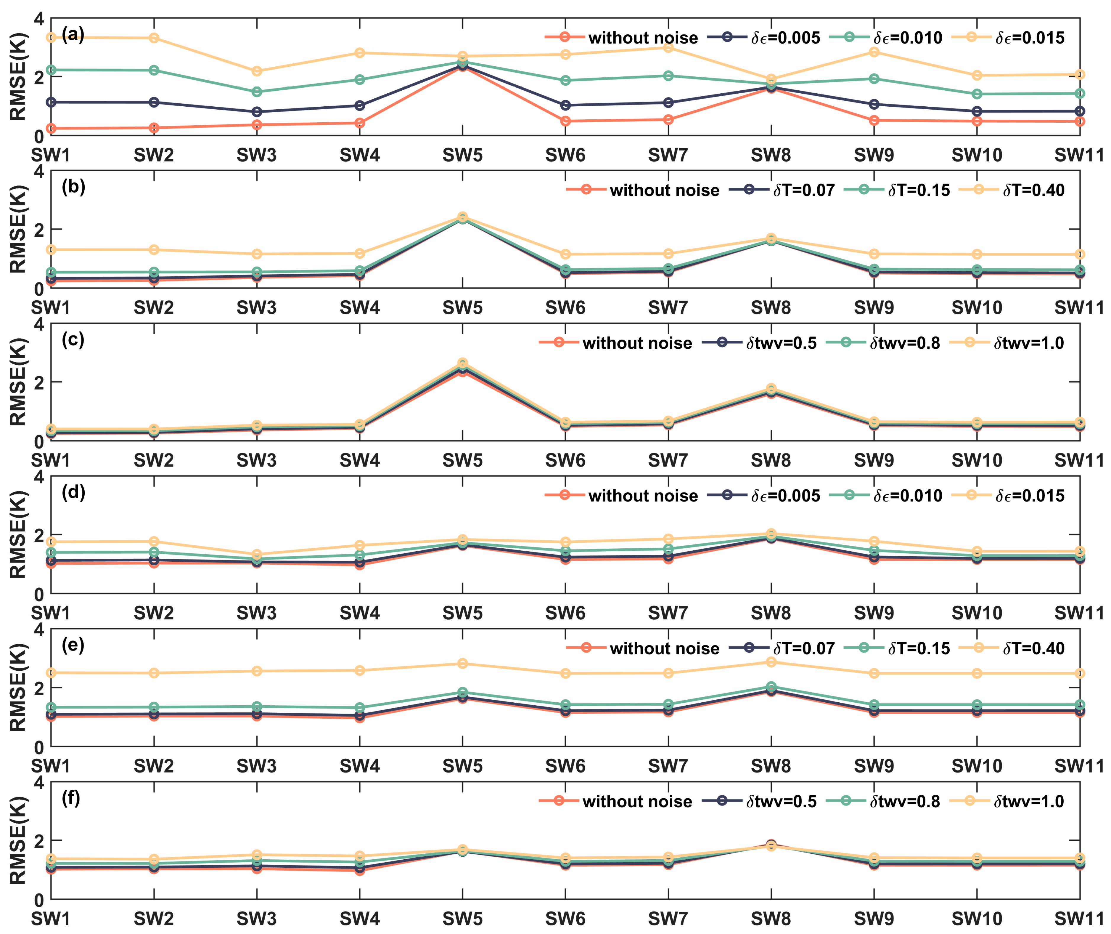
3.2. Sensitivity Analysis

The sensor noise, LSE, and TWV represent three principal sources of uncertainty that contribute to errors in LST retrieval [7,24]. To address this, we conducted an assessment of the sensitivity of the candidate SW algorithms to these three variables. The eleven candidate SW algorithm coefficients, calculated from the CLAR database, were tested with an independent dataset simulated using radiosounding profiles. Normal distributed random noise with a mean of 0 and a standard deviation of 0.07, 0.15, and 0.40 K was incorporated into the simulated TIRS-2 brightness temperature [58]. Furthermore, uncertainties of 0.005, 0.01, and 0.015 (unitless) and 0.5, 0.8, and 1.0 g/cm² were added to the LSE and TWV datasets, respectively [19]. Figure 2 shows the performance of the eleven candidate SW algorithms before and after the addition of random noise under different TWV subranges.

As illustrated in Figure 2a,d, the SW5 and SW8 algorithms exhibit the least sensitivity to emissivity uncertainty, while the SW10 and SW11 algorithms demonstrate the second-least sensitivity. In contrast, the SW1 and SW2 algorithms exhibit the greatest sensitivity to emissivity uncertainty. The LST uncertainty increases as the emissivity noise increases. This increase is more pronounced for lower TWV than for higher TWV. For example, when the emissivity uncertainty is 0.01, the RMSE of the SW2 algorithm increases from 0.27 K to 2.22 K and from 1.04 K to 1.41 K when the TWV is less than 1.5 g/cm² and greater than 4.5 g/cm², respectively. This suggests that the uncertainty in the emissivity has a more significant impact on the retrieval of the LST under dry atmospheric conditions, such as in northwest China and western Australia.

As shown in Figure 2b,e, when the uncertainty in the brightness temperature is equal to 0.15 K, the increase ratio of the RMSE is less than 0.5% for the majority of algorithms, with values above 1.0% for the SW1 and SW2 algorithms under a lower TWV subrange. Furthermore, as the TWV increases, the ratio of the increase declines. Based on the performance of on-orbit calibrations, the noise level in both channels of TIRS-2 is below 0.1 K [15,67]. Therefore, the uncertainty in the brightness temperature has a slight impact on the retrieval of the LST, both in dry and humid atmospheric conditions.

As indicated in Figure 2c,f, when the uncertainty in the TWV is less than 1.0 g/cm², the increase ratio of the RMSE is less than 0.6% for the eleven candidate algorithms. In other words, the uncertainty in the TWV has a negligible effect on the retrieval of the LST. But as indicated in previous research [24,68], the incorrect selection of the TWV subrange led to a significant increase in LST retrieval. For example, when the TWV were below 1.5 g/cm², the bias and RMSE for the SW2 algorithm were 0.0 K and 0.41 K, respectively. However, when a subrange of coefficients spanning 1.5–3.0 g/cm² was employed, the values shifted to −0.66 K and 0.79 K, respectively.

3.3. T-Based Validation Results

Figure 3 presents the bias and RMSE between the retrieved Landsat 9 LST and the in situ LST for all the matchups at the SURFRAD sites. After removing invalid matchups affected by clouds and cloud shadows based on the Landsat level-2 pixel quality channel, 234 matchups were obtained at the SURFRAD sites. In addition, the official Landsat 9 LST that was retrieved by the RTE algorithm was also validated. As illustrated in Figure 3, the Landsat 9 LSTs retrieved using the SW algorithm achieved a lower RMSE than those retrieved using the RTE algorithm when compared to the ground measurements, except for the PSU site. The GWN and SXF sites had a root mean square error (RMSE) of approximately 1.3 and 1.6 K, followed by the BND, PSU, and DRA sites with an RMSE ranging between 2.0 and 2.7 K. The FPK and TBL sites achieved an RMSE above 5.0 K for most of the SW algorithms. The RTE algorithm performed slightly better than the SW algorithm regarding the RMSE at the PSU station and provided consistently worse results at the other stations. In terms of the average difference (bias) between the retrieved Landsat 9 LST and the in situ LST, the Landsat 9 LST retrieved from the SW algorithm were underestimated at the PSU, GWN, and DRA sites. Conversely, the corresponding LSTs were overestimated at the BND, SXF, TBL, and FPK sites. However, the RTE algorithm underestimated the LST at the PSU site and overestimated it elsewhere.

The validation results above indicate that the candidate SW algorithm is suitable for estimating the LST from the Landsat 9 TIR data. There was no significant difference between the eleven candidate SW algorithms, with overall biases and RMSEs ranging from 1.44 to 1.61 K and 3.50 to 3.73 K, whereas these values were 2.82 K and 4.69 K for the RTE algorithm.

4. Discussion

Since March 2023, Landsat 9 Collection 2 data have been reprocessed based on the initial calibration results, which may affect the accuracy of the retrieved LST. Based on the research of Niclòs et al. [15], the official LST product retrieved with the original and reprocessed TIRS-2 data have similar accuracy in Valencia, but a systematic difference of about −0.6 K was observed for the SW LST. We also calculated the statistics between the official Landsat 9 LST product and the in situ LST obtained at the SURFRAD sites. The bias (RMSE) for the original and reprocessed TIRS-2 data were 1.44 (2.94) K and 1.42 (2.93) K. The validation result in Section 3 indicates that the SW algorithm can achieve a more accurate LST than the RTE algorithm, which is consistent with previous conclusions [11,19]. The uncertainty of the LST algorithm at the DRA, FPK, and TBL sites was greater than 2.5 K, which can be explained by the spatial heterogeneity in the cover types [64]. After excluding three sites with high spatial heterogeneity, the overall biases (RMSEs) of the Landsat 9 LSTs were between −0.18 (1.65) and 0.07 (1.71) K for the SW algorithms, while the bias and RMSE were 1.06 K and 2.38 K, respectively, for the RTE algorithm.

To assess the accuracy of the retrieved Landsat 9 LSTs at the FPK and TBL sites, we used the MODIS LSTs produced by the Temperature-Emissivity Separation (TES) algorithms as a reference for evaluating the performance of the retrieved LSTs. Figure 4 presents the cross-validation result for Landsat 9 LST at the FPK and TBL sites. It can be seen that the retrieved Landsat 9 LSTs have higher uncertainties during the summer months. The RMSEs range from 3.00 to 3.30 K at the FPK site and from 2.36 to 2.71 K at the TBL site for the SW algorithms, while the values are 3.96 K and 3.00 K for the RTE algorithm. As for the bias, the values are between −0.72 K and 0.37 K for the SW algorithms, but the biases are 3.08 K and 2.34 K for the RTE algorithm. It seems that the imprecise LSE could be the reason for the poor performance of the official Landsat 9 LST. Because the official LSEs at the FPK and TBL sites were invariant with the change in the NDVIs, they were unable to accurately reflect the changes in the vegetation cover over time [69,70]. In contrast to the summer, the validation results for the different algorithms show similar accuracy in the autumn, with an RMSE of about 1.20 K. Figure 5 shows the spatial distribution of the difference between the retrieved Landsat 9 LST and the MODIS LST at the FPK site (Figure 5a–d) and the TBL site (Figure 5e–h). As shown in Figure 5, the discrepancies between the MODIS LST and the Landsat 9 LST retrieved by the SW1 and SW3 algorithms exhibit a comparable spatial distribution. Conversely, the differences between the MODIS LST and the Landsat 9 LST retrieved by the SW5 (RTE) algorithm are more pronounced than those retrieved by the SW1 and SW3 algorithms in most regions. The 25th (75th) percentiles of the LST discrepancy between the MODIS LST and the Landsat 9 LST retrieved from the RTE, SW1, SW3, and SW5 algorithms are 0.28 (1.52), −0.66 (0.80),−0.78 (0.69), and −1.13 (0.27) K, respectively, whereas the corresponding values are −0.17 (0.94), −0.72 (0.65),−0.84 (0.54), and −0.57 (0.80) K for Figure 5e–h. The statistical results show that the SW algorithms can achieve more accurate Landsat 9 LSTs than the RTE algorithm compared with the MODIS LST, which is also consistent with previous research [11,15,19].

5. Conclusions

The LST is one of the key parameters in the Earth’s surface energy on regional and global scales. In this paper, we have adapted eleven candidate SW algorithms for LST retrieval from Landsat 9 TIRS-2 data. First, the coefficients of the SW algorithms were derived from the simulation dataset constructed using MODTRAN, emissivity spectra, and different global atmospheric profiles. Simulated data sets derived from CLAR, ERA5, GAPRI, SeeBor, and TIGR were used to calculate the coefficients, while the radiosonde profiles collected from global radiosonde stations were used independently for validation purposes. The NDVI threshold method was then used to estimate the Landsat 9 LSE to facilitate LST retrieval. Finally, the effectiveness of the SW algorithms was assessed using ground measurements collected from SURFRAS sites. The main findings are summarized below:

(1)

Any of the five atmospheric profile databases can be used for simulation when the TWV is less than 4.5 g/cm². However, the GAPRI profile is recommended for simulation when the TWV is greater than 4.5 g/cm². The SW5 and SW8 algorithms that do not depend on the emissivity difference exhibit the least sensitivity to emissivity uncertainty but with larger uncertainty in LST retrieval than other SW algorithms.

(2)

At the SURFRAD sites, the candidate SW algorithms exhibit comparable performance, with overall bias (RMSEs) ranging from 1.44 (3.50) to 1.61 (3.73) K compared to 2.82 K and 4.69 K for the RTE algorithm. As most of the TWVs at the SURFRAD sites were below 3.0 g/cm², more ground measurements with higher TWVs are needed to characterize the performance of the SW algorithms under different atmospheric conditions.

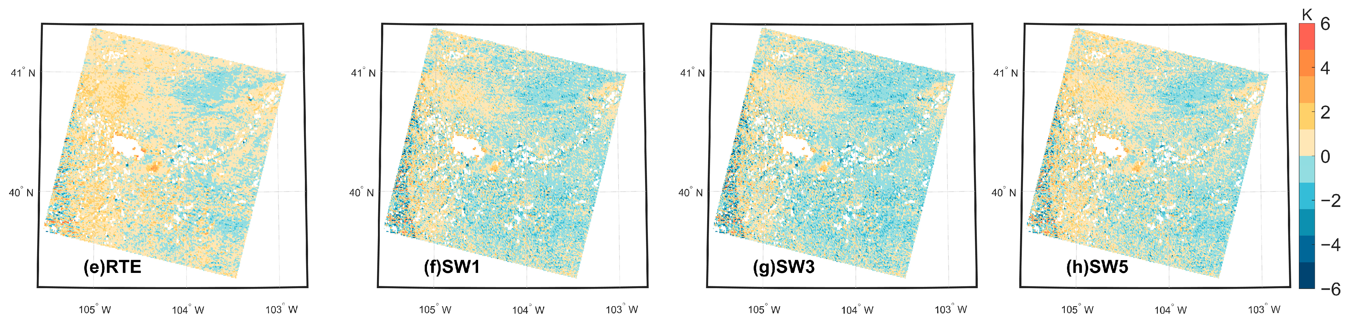
(3)

The consistency of the differences between the MODIS and Landsat LSTs indicates the stability of the SW algorithms over the seasons. The cross-validation results also indicated that the SW algorithms can achieve more accurate Landsat 9 LSTs than the RTE algorithm. This study provides an alternative method for the estimation of Landsat 9 LSTs.

References

- Hulley, G.C.; Hughes, C.G.; Hook, S.J. Quantifying uncertainties in land surface temperature and emissivity retrievals from aster and modis thermal infrared data. J. Geophys. Res. Atmos. 2012, 117, D23. [Google Scholar] [CrossRef]
- Göttsche, F.-M.; Olesen, F.-S.; Trigo, I.; Bork-Unkelbach, A.; Martin, M. Long term validation of land surface temperature retrieved from msg/seviri with continuous in-situ measurements in africa. Remote Sens. 2016, 8, 410. [Google Scholar] [CrossRef]
- Li, H.; Wang, H.; Yang, Y.; Du, Y.; Cao, B.; Bian, Z.; Liu, Q. Evaluation of atmospheric correction methods for the aster temperature and emissivity separation algorithm using ground observation networks in the hiwater experiment. IEEE Trans. Geosci. Remote Sens. 2019, 57, 3001–3014. [Google Scholar] [CrossRef]
- Sobrino, J.A.; Julien, Y.; Jiménez-Muñoz, J.-C.; Skokovic, D.; Sòria, G. Near real-time estimation of sea and land surface temperature for msg seviri sensors. Int. J. Appl. Earth Obs. Geoinf. 2020, 89, 102096. [Google Scholar] [CrossRef]
- Trigo, I.F.; Ermida, S.L.; Martins, J.P.A.; Gouveia, C.M.; Göttsche, F.-M.; Freitas, S.C. Validation and consistency assessment of land surface temperature from geostationary and polar orbit platforms: Seviri/msg and avhrr/metop. ISPRS J. Photogramm. Remote Sens. 2021, 175, 282–297. [Google Scholar] [CrossRef]
- Valor, E.; Caselles, V. Mapping land surface emissivity from ndvi: Application to european, african, and south american areas. Remote Sens. Environ. 1996, 57, 167–184. [Google Scholar] [CrossRef]
- Wan, Z.; Dozier, J. A generalized split-window algorithm for retrieving land-surface temperature from space. IEEE Trans. Geosci. Remote Sens. 1996, 34, 892–905. [Google Scholar]
- Zeng, Q.; Cheng, J.; Yue, W. Estimating hourly all-sky surface longwave upward radiation using the new generation of chinese geostationary weather satellites fengyun-4a/agri. IEEE Trans. Geosci. Remote Sens. 2024, 62, 1–12. [Google Scholar] [CrossRef]
- Eon, R.; Gerace, A.; Falcon, L.; Poole, E.; Kleynhans, T.; Raqueño, N.; Bauch, T. Validation of landsat-9 and landsat-8 surface temperature and reflectance during the underfly event. Remote Sens. 2023, 15, 3370. [Google Scholar] [CrossRef]
- Meng, X.; Cheng, J.; Guo, H.; Guo, Y.; Yao, B. Accuracy evaluation of the landsat 9 land surface temperature product. IEEE J. Sel. Top. Appl. Earth Obs. Remote Sens. 2022, 15, 8694–8703. [Google Scholar] [CrossRef]
- Wang, M.; Li, M.; Zhang, Z.; Hu, T.; He, G.; Zhang, Z.; Wang, G.; Li, H.; Tan, J.; Liu, X. Land surface temperature retrieval from landsat 9 tirs-2 data using radiance-based split-window algorithm. IEEE J. Sel. Top. Appl. Earth Obs. Remote Sens. 2023, 16, 1100–1112. [Google Scholar] [CrossRef]
- Masek, J.G.; Wulder, M.A.; Markham, B.; McCorkel, J.; Crawford, C.J.; Storey, J.; Jenstrom, D.T. Landsat 9: Empowering open science and applications through continuity. Remote Sens. Environ. 2020, 248, 111968. [Google Scholar] [CrossRef]
- Montanaro, M.; McCorkel, J.; Tveekrem, J.; Stauder, J.; Mentzell, E.; Lunsford, A.; Hair, J.; Reuter, D. Landsat 9 thermal infrared sensor 2 (tirs-2) stray light mitigation and assessment. IEEE Trans. Geosci. Remote Sens. 2022, 60, 1–8. [Google Scholar] [CrossRef]
- Xu, H.; Ren, M.; Lin, M. Cross-comparison of landsat-8 and landsat-9 data: A three-level approach based on underfly images. GIScience Remote Sens. 2024, 61, 2318071. [Google Scholar] [CrossRef]
- Niclòs, R.; Perelló, M.; Puchades, J.; Coll, C.; Valor, E. Evaluating landsat-9 tirs-2 calibrations and land surface temperature retrievals against ground measurements using multi-instrument spatial and temporal sampling along transects. Int. J. Appl. Earth Obs. Geoinf. 2023, 125, 103576. [Google Scholar] [CrossRef]
- Jiménez-Muñoz, J.C.; Sobrino, J.A.; Skokovic, D.; Mattar, C.; Cristobal, J. Land surface temperature retrieval methods from landsat-8 thermal infrared sensor data. IEEE Geosci. Remote Sens. Lett. 2014, 11, 1840–1843. [Google Scholar] [CrossRef]
- Rozenstein, O.; Qin, Z.; Derimian, Y.; Karnieli, A. Derivation of land surface temperature for landsat-8 tirs using a split window algorithm. Sensors 2014, 14, 5768–5780. [Google Scholar] [CrossRef]
- Caselles, V.; Rubio, E.; Coll, C.; Valor, E. Thermal band selection for the prism instrument 3. Optimal band configurations. J. Geophys. Res. 1998, 103, 17057–17067. [Google Scholar] [CrossRef]
- Ye, X.; Ren, H.; Zhu, J.; Fan, W.; Qin, Q. Split-window algorithm for land surface temperature retrieval from landsat-9 remote sensing images. IEEE Geosci. Remote Sens. Lett. 2022, 19, 1–5. [Google Scholar] [CrossRef]
- Ye, X.; Liu, R.; Hui, J.; Zhu, J. Land surface temperature estimation from landsat-9 thermal infrared data using ensemble learning method considering the physical radiance transfer process. Land 2023, 12, 1287. [Google Scholar] [CrossRef]
- Zhou, J.; Liang, S.; Cheng, J.; Wang, Y.; Ma, J. The glass land surface temperature product. IEEE J. Sel. Top. Appl. Earth Obs. Remote Sens. 2019, 12, 493–507. [Google Scholar] [CrossRef]
- Yu, Y.; Privette, J.L.; Pinheiro, A.C. Evaluation of split-window land surface temperature algorithms for generating climate data records. IEEE Trans. Geosci. Remote Sens. 2008, 46, 179–192. [Google Scholar] [CrossRef]
- Dong, L.; Tang, S.; Wang, F.; Cosh, M.; Li, X.; Min, M. Inversion and validation of fy-4a official land surface temperature product. Remote Sens. 2023, 15, 2437. [Google Scholar] [CrossRef]
- Meng, X.; Cheng, J.; Zhao, S.; Liu, S.; Yao, Y. Estimating land surface temperature from landsat-8 data using the noaa jpss enterprise algorithm. Remote Sens. 2019, 11, 155. [Google Scholar] [CrossRef]
- Meng, X.; Liu, W.; Cheng, J.; Guo, H. An operational split-window algorithm for retrieving land surface temperature from fengyun-4a agri data. Remote Sens. Lett. 2023, 14, 1206–1217. [Google Scholar] [CrossRef]
- Becker, F.; Li, Z.-L. Towards a local split window method over land surfaces. Int. J. Remote Sens. 1990, 11, 369–393. [Google Scholar] [CrossRef]
- Wan, Z. New refinements and validation of the collection-6 modis land-surface temperature/emissivity product. Remote Sens. Environ. 2014, 140, 36–45. [Google Scholar] [CrossRef]
- Price, J.C. Land surface temperature measurements from the split window channels of the noaa 7 advanced very high resolution radiometer. J. Geophys. Res. Atmos. 1984, 89, 7231–7237. [Google Scholar] [CrossRef]
- Yu, Y.; Liu, Y.; Yu, P.; Wang, H. Enterprise Algorithm Theoretical Basis Document for Viirs Land Surface Temperature Production, version 1.0; NOAA: Silver Spring, MD, USA, 2017. [Google Scholar]
- Caselles, V.; Coll, C.; Valor, E. Land surface emissivity and temperature determination in the whole hapex-sahel area from avhrr data. Int. J. Remote Sens. 1997, 18, 1009–1027. [Google Scholar] [CrossRef]
- Ulivieri, C.; Castronuovo, M.; Francioni, R.; Cardillo, A. A split window algorithm for estimating land surface temperature from satellites. Adv. Space Res. 1994, 14, 59–65. [Google Scholar] [CrossRef]
- Vidal, A. Atmospheric and emissivity correction of land surface temperature measured from satellite using ground measurements or satellite data. Int. J. Remote Sens. 1991, 12, 2449–2460. [Google Scholar] [CrossRef]
- Ulivieri, C.; Cannizzaro, G. Land surface temperature retrievals from satellite measurements. Acta Astronaut. 1985, 12, 977–985. [Google Scholar] [CrossRef]
- Sobrino, J.A.; Li, Z.-L.; Stoll, M.P.; Becker, F. Improvements in the split-window technique for land surface temperature determination. IEEE Trans. Geosci. Remote Sens. 1994, 32, 243–253. [Google Scholar] [CrossRef]
- Coll, C.; Valor, E.; Schmugge, T.; Caselles, V. A procedure for estimating the land surface emissivity difference in the avhrr channels 4 and 5. Remote Sens. Appl. Valencia. Area 1997. [Google Scholar]
- Sobrino, J.; Li, Z.; Stoll, M.P.; Becker, F. Determination of the surface temperature from atsr data. In Proceedings of the 25th International Symposium on Remote Sensing of Environment, Graz, Austria, 4–8 April 1993; ERIM: Rotterdam, Netherlands, 1993; pp. 4–8. [Google Scholar]
- Emami, H.; Mojaradi, B.; Safari, A. A new approach for land surface emissivity estimation using ldcm data in semi-arid areas: Exploitation of the aster spectral library data set. Int. J. Remote Sens. 2016, 37, 5060–5085. [Google Scholar] [CrossRef]
- Cheng, J.; Liang, S.; Verhoef, W.; Shi, L.; Liu, Q. Estimating the hemispherical broadband longwave emissivity of global vegetated surfaces using a radiative transfer model. IEEE Trans. Geosci. Remote Sens. 2016, 54, 905–917. [Google Scholar] [CrossRef]
- Tang, B.H.; Shao, K.; Li, Z.L.; Wu, H.; Tang, R. An improved ndvi-based threshold method for estimating land surface emissivity using modis satellite data. Int. J. Remote Sens. 2015, 36, 4864–4878. [Google Scholar] [CrossRef]
- Meng, X.; Guo, H.; Cheng, J.; Yao, B. Can the era5 reanalysis product improve the atmospheric correction accuracy of landsat series thermal infrared data? IEEE Geosci. Remote Sens. Lett. 2022, 19, 7506805. [Google Scholar] [CrossRef]
- Meng, X.; Liu, W.; Cheng, J.; Guo, H.; Yao, B. Estimating hourly land surface temperature from fy-4a agri using an explicitly emissivity-dependent split-window algorithm. IEEE J. Sel. Top. Appl. Earth Obs. Remote Sens. 2023, 16, 5474–5487. [Google Scholar] [CrossRef]
- Aires, F.; Chédin, A.; Scott, N.A.; Rossow, W.B. A regularized neural net approach for retrieval of atmospheric and surface temperatures with the iasi instrument. J. Appl. Meteorol. Climatol. 2001, 41, 144–159. [Google Scholar] [CrossRef]
- Mattar, C.; Durán-Alarcón, C.; Jiménez-Muñoz, J.C.; Santamaría-Artigas, A.; Olivera-Guerra, L.; Sobrino, J.A. Global atmospheric profiles from reanalysis information (gapri): A new database for earth surface temperature retrieval. Int. J. Remote Sens. 2015, 36, 5045–5060. [Google Scholar] [CrossRef]
- Borbas, E.E.; Seemann, S.W.; Huang, H.L.; Li, J.; Menzel; Paul, W. Global Profile Training Database for Satellite Regression Retrievals with Estimates of Skin Temperature and Emissivity. In Proceedings of the International ATOVS Study Conference-XIV, Beijing, China, 25–31 May 2005; University of Wisconsin—Madison: Madison, WI, USA, 2005; pp. 763–770. [Google Scholar]
- Galve, J.M.; Coll, C.; Caselles, V.; Valor, E. An atmospheric radiosounding database for generating land surface temperature algorithms. IEEE Trans. Geosci. Remote Sens. 2008, 46, 1547–1557. [Google Scholar] [CrossRef]
- Jiang, G.-M.; Zhou, W.; Liu, R. Development of split-window algorithm for land surface temperature estimation from the virr/fy-3a measurements. IEEE Geosci. Remote Sens. Lett. 2013, 10, 952–956. [Google Scholar] [CrossRef]
- Meng, X.; Cheng, J.; Liang, S. Estimating land surface temperature from feng yun-3c/mersi data using a new land surface emissivity scheme. Remote Sens. 2017, 9, 1247. [Google Scholar] [CrossRef]
- Tang, B.-H. Nonlinear split-window algorithms for estimating land and sea surface temperatures from simulated chinese gaofen-5 satellite data. IEEE Trans. Geosci. Remote Sens. 2018, 56, 6280–6289. [Google Scholar] [CrossRef]
- Ma, J.; Zhou, J.; Göttsche, F.-M.; Liang, S.; Wang, S.; Li, M. A global long-term (1981–2000) land surface temperature product for noaa avhrr. Earth Syst. Sci. Data 2020, 12, 3247–3268. [Google Scholar] [CrossRef]
- Li, H.; Yang, Y.; Li, R.; Wang, H.; Cao, B.; Bian, Z.; Hu, T.; Du, Y.; Sun, L.; Liu, Q. Comparison of the musyq and modis collection 6 land surface temperature products over barren surfaces in the heihe river basin, china. IEEE Trans. Geosci. Remote Sens. 2019, 57, 8081–8094. [Google Scholar] [CrossRef]
- Niclòs, R.; Galve, J.M.; Valiente, J.A.; Estrela, M.J.; Coll, C. Accuracy assessment of land surface temperature retrievals from msg2-seviri data. Remote Sens. Environ. 2011, 115, 2126–2140. [Google Scholar] [CrossRef]
- Tang, K.; Zhu, H.; Ni, P.; Li, R.; Fan, C. Retrieving land surface temperature from chinese fy-3d mersi-2 data using an operational split window algorithm. IEEE J. Sel. Top. Appl. Earth Obs. Remote Sens. 2021, 14, 6639–6651. [Google Scholar] [CrossRef]
- Ermida, S.L.; Trigo, I.F. A comprehensive clear-sky database for the development of land surface temperature algorithms. Remote Sens. 2022, 14, 2329. [Google Scholar] [CrossRef]
- Zhang, G.; Li, D.; Li, H.; Xu, Z.; Hu, Z.; Zeng, J.; Yang, Y.; Jia, H. Improving hj-1b/irs lst retrieval of the generalized single-channel algorithm with refined era5 atmospheric profile database. Remote Sens. 2023, 15, 5092. [Google Scholar] [CrossRef]
- Meng, X.; Cheng, J. Evaluating eight global reanalysis products for atmospheric correction of thermal infrared sensor—Application to landsat 8 tirs10 data. Remote Sens. 2018, 10, 474. [Google Scholar] [CrossRef]
- Meng, X.; Cheng, J. Estimating land and sea surface temperature from cross-calibrated chinese gaofen-5 thermal infrared data using split-window algorithm. IEEE Geosci. Remote Sens. Lett. 2020, 17, 509–513. [Google Scholar] [CrossRef]
- Meng, Y.; Zhou, J.; Göttsche, F.-M.; Tang, W.; Martins, J.; Perez-Planells, L.; Ma, J.; Wang, Z. Investigation and validation of two all-weather land surface temperature products with in-situ measurements. Geo-Spat. Inf. Sci. 2023, 27, 670–682. [Google Scholar] [CrossRef]
- Sayler, K.; Glynn, T. Landsat 9 Data Users Handbook; Earth Resources Observation and Science (EROS) Center: Sioux Falls, SD, USA, 2022. Available online: https://www.usgs.gov/media/files/landsat-9-data-users-handbook (accessed on 1 June 2024).
- Zhang, Z.; He, G.; Wang, M.; Long, T.; Wang, G.; Zhang, X. Validation of the generalized single-channel algorithm using landsat 8 imagery and surfrad ground measurements. Remote Sens. Lett. 2016, 7, 810–816. [Google Scholar] [CrossRef]
- Duan, S.-B.; Li, Z.-L.; Li, H.; Göttsche, F.-M.; Wu, H.; Zhao, W.; Leng, P.; Zhang, X.; Coll, C. Validation of collection 6 modis land surface temperature product using in situ measurements. Remote Sens. Environ. 2019, 225, 16–29. [Google Scholar] [CrossRef]
- Martin, M.; Ghent, D.; Pires, A.; Göttsche, F.-M.; Cermak, J.; Remedios, J. Comprehensive in situ validation of five satellite land surface temperature data sets over multiple stations and years. Remote Sens. 2019, 11, 479. [Google Scholar] [CrossRef]
- Zeng, Q.; Cheng, J.; Sun, H.; Dong, S. An integrated framework for estimating the hourly all-time cloudy-sky surface long-wave downward radiation for fengyun-4a/agri. Remote Sens. Environ. 2024, 312, 114319. [Google Scholar] [CrossRef]
- Guillevic, P.C.; Biard, J.C.; Hulley, G.C.; Privette, J.L.; Hook, S.J.; Olioso, A.; Göttsche, F.M.; Radocinski, R.; Román, M.O.; Yu, Y.; et al. Validation of land surface temperature products derived from the visible infrared imaging radiometer suite (viirs) using ground-based and heritage satellite measurements. Remote Sens. Environ. 2014, 154, 19–37. [Google Scholar] [CrossRef]
- Malakar, N.K.; Hulley, G.C.; Hook, S.J.; Laraby, K.; Cook, M.; Schott, J.R. An operational land surface temperature product for landsat thermal data: Methodology and validation. IEEE Trans. Geosci. Remote Sens. 2018, 56, 5717–5735. [Google Scholar] [CrossRef]
- Ma, J.; Zhou, J.; Göttsche, F.-M.; Wang, Z.; Wu, H.; Tang, W.; Li, M.; Liu, S. An atmospheric influence correction method for longwave radiation-based in-situ land surface temperature. Remote Sens. Environ. 2023, 293, 113611. [Google Scholar] [CrossRef]
- Cheng, J.; Liang, S.; Yao, Y.; Zhang, X. Estimating the optimal broadband emissivity spectral range for calculating surface longwave net radiation. IEEE Geosci. Remote Sens. Lett. 2013, 10, 401–405. [Google Scholar] [CrossRef]
- Barsi, J.A.; Montanaro, M.; Thome, K.; Raqueno, N.G.; Hook, S.; Anderson, C.H.; Micijevic, E. Early Radiometric Performance of Landsat-9 Thermal Infrared Sensor. In Proceedings of the Earth Observing Systems XXVII, San Diego, CA, USA, 21–26 August 2022; SPIE: Washington, DC, USA, 2022; pp. 223–233. [Google Scholar]
- Du, C.; Ren, H.; Qin, Q.; Meng, J.; Zhao, S. A practical split-window algorithm for estimating land surface temperature from landsat 8 data. Remote Sens. 2015, 7, 647–665. [Google Scholar] [CrossRef]
- Duan, S.-B.; Li, Z.-L.; Zhao, W.; Wu, P.; Huang, C.; Han, X.-J.; Gao, M.; Leng, P.; Shang, G. Validation of landsat land surface temperature product in the conterminous united states using in situ measurements from surfrad, arm, and ndbc sites. Int. J. Digit. Earth 2021, 14, 640–660. [Google Scholar] [CrossRef]
- Cheng, J.; Meng, X.; Dong, S.; Liang, S. Generating the 30-m land surface temperature product over continental china and USA from landsat 5/7/8 data. Sci. Remote Sens. 2021, 4, 100032. [Google Scholar] [CrossRef]