A Fast Two-Dimensional Direction-of-Arrival Estimator Using Array Manifold Matrix Learning

Abstract

Sparsity-based methods for two-dimensional (2D) direction-of-arrival (DOA) estimation often suffer from high computational complexity due to the large array manifold dictionaries. This paper proposes a fast 2D DOA estimator using array manifold matrix learning, where source-associated grid points are progressively selected from the set of predefined angular grids based on marginal likelihood maximization in the sparse Bayesian learning framework. This grid selection reduces the size of the manifold dictionary matrix, avoiding large-scale matrix inversion and resulting in reduced complexity. To overcome grid mismatch errors, grid optimization is established based on the marginal likelihood, with a dichotomizing-based solver provided that is applicable to arbitrary planar arrays. For uniform rectangular arrays, we present a 2D zoom fast Fourier transform as an alternative to the dichotomizing-based solver by transforming the manifold vector in a specific form, thus accelerating the computation without compromising accuracy. Simulation results verify the superior performance of the proposed methods in terms of estimation accuracy, computational efficiency, and angle resolution compared to state-of-the-art methods for 2D DOA estimation.

1. Introduction

Direction-of-arrival (DOA) estimation plays a crucial role in various fields such as sonar, radar, and wireless communications [1]. Classical subspace-based methods, including multiple signal classification (MUSIC) [2] and estimation parameter via rotational invariance technique (ESPRIT) [3], face performance degradation in scenarios with a low signal-to-noise ratio (SNR) or limited snapshots [4]. To address this issue, sparse representation (SR) methods [5,6,7,8,9,10,11,12] have emerged as a promising solution. By exploiting the spatial sparsity of the source signals, SR methods transform the DOA estimation problem into the sparse signal recovery problem. The locations of the peaks of recovered signals indicate the source DOAs.

On-grid SR methods [5,6,7,8] employ an overcomplete array manifold dictionary across a set of predefined angular grids in sparse parameter estimation. However, grid mismatch, arising from the discrepancies between source DOAs and predefined grids, can degrade the estimation accuracy of on-grid SR methods. To mitigate this problem, off-grid SR methods [8,9,10,11,12] that integrate a grid refinement process have been proposed. Off-grid SR methods iteratively adjust the grids, enabling DOA estimates to approach the source DOAs, thereby improving the estimation accuracy. One major limitation of many grid-based methods is the high computational complexity due to the large size of the manifold dictionary matrix. Most existing grid-based SR methods focus on the one-dimensional (1D) DOA estimation.

For two-dimensional (2D) DOA estimation, where both azimuth and elevation angles are estimated, the 2D counterparts of 1D grid-based SR methods typically have significantly increased computational demand due to the larger manifold dictionary. Therefore, fast SR methods with low complexity have become a focal point in 2D DOA estimation. An efficient SR-based combination method, called SAMV-RELAX, is proposed in [13] by utilizing the sparse asymptotic minimum variance (SAMV) method [8] for initial sparse parameter estimation, followed by the RELAX approach [14] for refinement. SAMV-RELAX achieves good computational efficiency by employing coarse 2D angular grids. In contrast, another fast gridless maximum likelihood (FGML) method [15] effectively retrieves source DOAs by processing the reconstructed covariance matrix using the 2D MUSIC or 2D ESPRIT algorithms [16]. By deriving a closed-form formula for covariance matrix reconstruction, FGML exhibits favorable computational efficiency. However, both SAMV-RELAX and FGML methods require knowledge of the source number for parameter estimation, which can limit their performance in practical situations.

A recently proposed method, marginal likelihood maximization-based fast array manifold matrix learning (FAMML) [17], achieves low-complexity 1D DOA estimation within the sparse Bayesian learning (SBL) framework [18,19]. This method incrementally learns source-associated angles and forms a small-size manifold matrix during estimation, avoiding large-scale matrix inversion. Each learned angle is identified from predefined grids and is subsequently optimized to overcome grid mismatch, yielding high estimation accuracy. Given these advantages, the 2D extension of FAMML holds significant research value. However, the extension faces challenges as grid optimization becomes more complicated due to azimuth–elevation coupling.

Inspired by the FAMML method [17], a fast 2D DOA estimator for planar arrays is developed in this study, where predefined 2D angular grids are selected one by one for marginal likelihood maximization, rather than being used simultaneously. This grid selection reduces the size of the manifold dictionary matrix, avoiding the need for large-scale matrix inversion. To achieve a more accurate value of the selected grid point, an efficient dichotomizing-based grid optimization is established, iteratively refining the grid within a bounded area that shrinks with each iteration. This method is applicable to arbitrary planar arrays. For uniform rectangular arrays (URAs), we further express the grid optimization objective function in a 2D fast Fourier transform (FFT) form by exploiting the Kronecker structure of the manifold vector. This enables employing a 2D zoom-FFT [20] for grid optimization, accelerating the computation without compromising estimation accuracy.

The proposed DOA estimator extends the FAMML method in [17] from 1D to 2D DOA estimation, preserving low complexity while achieving high estimation accuracy. The primary contributions of this work are as follows:

(1)

The proposal of a 2D angular grid optimization for arbitrary planar arrays, where the selected grid is iteratively refined using a dichotomizing method, improving estimation accuracy.

(2)

The proposal of an enhanced-efficiency grid optimization for URAs: The utilization of the 2D zoom-FFT, exploiting the Kronecker structure of the manifold vector, accelerates the computation in grid optimization.

The remainder of this paper is organized as follows. Section 2 presents the signal model for 2D DOA estimation. In Section 3, the proposed 2D fast DOA estimator is introduced in detail. The numerical simulations are conducted in Section 4, and conclusions are drawn in Section 5.

Notation: Bold symbols in small and capital fonts represent the matrices and vectors, respectively. $\mathbb{C}$ stands for the set of complex numbers. ${(\cdot )}^T$, ${(\cdot )}^H$, and ${(\cdot )}^{\ast }$ are the transpose, conjugate transpose, and conjugate operators, respectively. ${(\cdot )}^{-1}$ and ${(\cdot )}^{†}$ are the matrix inverse and the Moore–Penrose pseudo-inverse, respectively. $\mathrm{diag}(\cdot )$ denotes the diagonal operator to create a diagonal matrix with a vector being the diagonal elements. $\Vert \cdot \Vert$, ${\Vert \cdot \Vert }_2$, and ${\Vert \cdot \Vert }_F$ denote the absolute value, ${\mathcal{l}}_2$ norm, and Frobenius norm, respectively. $\otimes$ denotes the Kronecker product. $\mathrm{Re}(\cdot )$ represents the real part of a complex vector. $\mathrm{size}(\cdot )$ represents the matrix size. $\mathrm{tr}(\cdot )$ denotes the trace of a matrix. ${\mathrm{vec}}^{-1}(\cdot )$ denotes the inverse operator of vectorization that returns a matrix. ${\cos }^{-1}(\cdot )$ and ${\sin }^{-1}(\cdot )$ denote the inverse cosine function and inverse sine function, respectively. The notation $\partial$ denotes the partial derivative operator. $\max (\cdot )$ represents the maximum value of one or more numbers or variables. $\gg$ is used to denote that one quantity is much greater than another. $\mathcal{C}\mathcal{N}(\cdot )$ represents the complex Gaussian distribution. $\mathcal{O}(\cdot )$ is used to describe the order of computational complexity. $\triangleq$ is used to indicate an exact definition or description of a term. The imaginary unit is denoted by $j=\sqrt{-1}$.

2. Signal Model

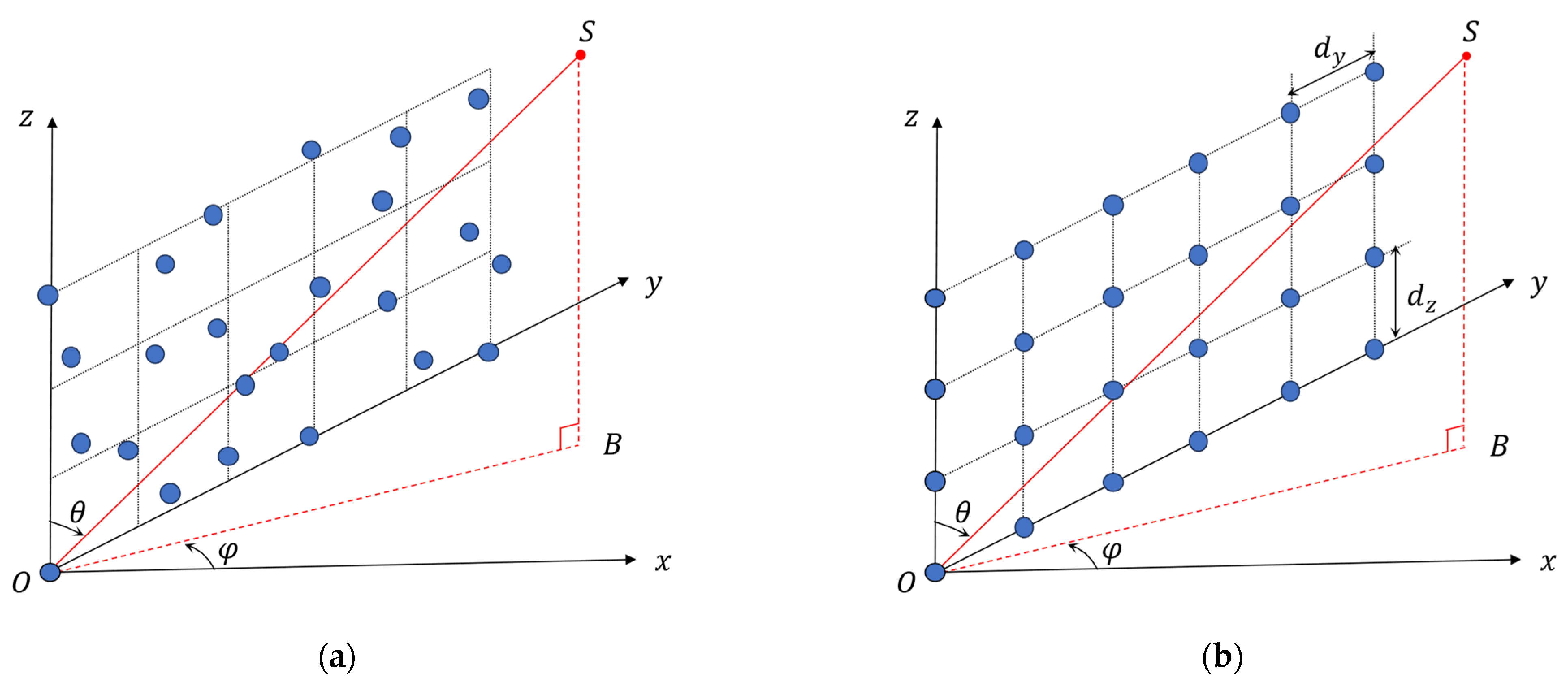
Consider a planar array composed of M sensors lying in the y–z plane. The position of array sensors in a Cartesian coordinate system is given by $r=[r_1,\cdots ,r_M]$, where $r_m={[0,y_m,z_m]}^T$, $m=1,\cdots ,M$. The configuration of the planar array is depicted in Figure 1. Let $\phi$ and $\theta$ denote the azimuth and elevation angles, respectively. The K narrowband far-field source signals arrival at the planar array from directions ${\Theta }_S\triangleq {\left\{{\Theta }_{Sk}\right\}}_{k=1}^K={\{({\theta }_{Sk},{\phi }_{Sk})\}}_{k=1}^K$, where ${\Theta }_{Sk}=({\theta }_{Sk},{\phi }_{Sk})$ is the kth source signal’s DOA. The array manifold vector of the kth signal is:

$$a({\Theta }_{Sk})={[\exp (j{\omega }_{1,k}),\cdots ,\exp (j{\omega }_{M,k})]}^T,$$

(1)

where ${\omega }_{m,k}=2\pi (y_m\sin {\theta }_{Sk}\sin {\phi }_{Sk}+z_m\cos {\theta }_{Sk})/\lambda$, $m=1,\cdots ,M$, $k=1,\cdots ,K$, and $\lambda$ is the signal wavelength.

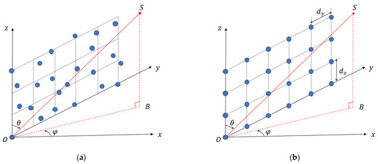
Figure 1. Configuration of the planar array: (a) arbitrary planar array; (b) URA. Blue dots represent array sensors; red dots represent the source position; B represents the projection of the source position onto the x–y plane.

The array output matrix $Y=[y(1),\cdots ,y(L)]\in {\mathbb{C}}^{M\times L}$ can be modeled as:

$$Y=A({\Theta }_S)X+N,$$

(2)

where L is the number of snapshots, $X=[x(1),\dots ,x(L)]\in {\mathbb{C}}^{K\times L}$ is the source signal matrix, $N=[n(1),\cdots ,n(L)]\in {\mathbb{C}}^{M\times L}$ is the additional white Gaussian noise matrix, and $A({\Theta }_S)=[a({\Theta }_{S1}),\cdots ,a({\Theta }_{SK})]\in {\mathbb{C}}^{M\times K}$ is the array manifold matrix.

To estimate 2D DOAs using sparse representation, the 2D spatial space is discretized into a set of 2D angular grids. One can define azimuth grids ${\left\{{\overline{\phi }}_i\right\}}_{i=1}^{Q_a}$ and elevation grids ${\left\{{\overline{\theta }}_j\right\}}_{j=1}^{Q_e}$ over the angle range, where $Q_a$ and $Q_e$ are the numbers of grid points. The set of 2D angular grids, containing $Q=Q_a{Q}_e$ elements, can be expressed as ${\Theta }_G=\{({\overline{\theta }}_1,{\overline{\phi }}_1),\cdots ,({\overline{\theta }}_1,{\overline{\phi }}_{Q_a}),({\overline{\theta }}_2,{\overline{\phi }}_1),\cdots ,({\overline{\theta }}_2,{\overline{\phi }}_{Q_a}),\cdots ,({\overline{\theta }}_{Q_e},{\overline{\phi }}_1),\cdots ,({\overline{\theta }}_{Q_e},{\overline{\phi }}_{Q_a})\}$. For convenience, the qth predefined grid is represented by ${\Theta }_{Gq}=({\theta }_{Gq},{\phi }_{Gq})$, $q=1,\cdots ,Q$. Then, the array output $Y$ can be sparsely represented over ${\Theta }_G$ as:

$$Y=A({\Theta }_G)\overline{X}+N,$$

(3)

where $A({\Theta }_G)=[a({\Theta }_{G1}),\cdots ,a({\Theta }_{GQ})]\in {\mathbb{C}}^{M\times Q}$ is the overcomplete manifold dictionary, and $\overline{X}=[\overline{x}(1),\dots ,\overline{x}(L)]\in {\mathbb{C}}^{Q\times L}$ is the sparse signal matrix, whose qth row represents a possible signal at $({\theta }_{Gq},{\phi }_{Gq})$, $q\in \{1,\cdots ,Q\}$. As the number of predefined grids is usually considerably larger than that of source signals, i.e., $Q\gg K$, only a few elements in $\overline{x}(t)$ are non-zero, and their locations indicate the DOA estimates.

3. The Proposed Fast 2D Estimation Using Array Manifold Matrix Learning

In this section, we address the 2D DOA estimation problem in the SBL framework, using an array manifold matrix learning process to achieve accurate, efficient estimates.

3.1. Bayesian Model

Assume that every column of the sparse signal matrix $\overline{X}$ adheres to a zero-mean complex Gaussian distribution with precision matrix (inverse covariance matrix) $\Lambda$, leading to:

$$P(\overline{X}|\alpha )=\prod _{t=1}^L\mathcal{C}\mathcal{N}(\overline{x}(t)|\mathbf{0},{\Lambda }^{-1}),$$

(4)

where $\Lambda =\mathrm{diag}(\alpha )$, and $\alpha ={[{\alpha }_1,\cdots ,{\alpha }_Q]}^T$ with ${\alpha }_q$ being the precision parameter (inverse variance) of the qth element in $\overline{x}(t)$, $q=1,\cdots ,Q$. Obviously, ${\alpha }_q\to \infty$ when no signal is located on the qth grid point ${\Theta }_{Gq}$.

Under the assumption of while Gaussian noise, the likelihood distribution of array output $Y$ given the signal matrix $\overline{X}$ can be expressed as follows:

$$P(Y|\overline{X}|{\Theta }_G,\beta )=\prod _{t=1}^L\mathcal{C}\mathcal{N}(y(t)|A({\Theta }_G)\overline{x}(t),{\beta }^{-1}{I}_M),$$

(5)

where $\beta$ is the noise precision and $I_M$ is the identity matrix of order M.

Based on the Bayes theory, the Gaussian posterior of distribution of $\overline{X}$ can be derived, expressed as:

$$P(\overline{X}|Y,\alpha ,{\Theta }_G,\beta )=\prod _{t=1}^L\mathcal{C}\mathcal{N}(\overline{x}(t)|\mu (t),\Sigma ),$$

(6)

where $\mu (t)$ and $\Sigma$ are the mean vector and covariance matrix, respectively, given by:

$$\left\{\begin{array}{l}\mu (t)=\beta \Sigma A^H({\Theta }_G)y(t),t=1,\cdots ,L\\ \Sigma ={\left(\Lambda +\beta A^H({\Theta }_G)A({\Theta }_G)\right)}^{-1}\end{array}\right..$$

(7)

As shown in (7), the computation of the posterior covariance $\Sigma$ involves a matrix inversion. However, due to the commonly large number of angular grids, the array manifold dictionary $A({\Theta }_G)$ is high-dimensional with the consequence that the matrix inversion is computationally expensive. Thus, the conventional SBL method often has a high computational complexity in the iterative parameter estimation.

3.2. Parameter Estimation Using Array Manifold Matrix Learning

Inspired by the array manifold matrix learning process in [17], the proposed DOA estimator progressively activates predefined grids and uses them within the parameter estimation process, avoiding the need for large-scale matrix inversion.

3.2.1. Criterion on Active Grid Selection

The proposed DOA estimator activates predefined grids in ${\Theta }_G$ one by one during iterations. These activated grids are referred to as “active grids”, whose grid indexes compose a set, denoted by ${\mathcal{I}}_{active}$. The number of active grids is denoted by $\tilde{K}$. All active grids construct an “active set”, denoted by ${\Theta }_{active}$ and given by:

$${\Theta }_{active}=\{({\theta }_{Gi},{\phi }_{Gi}): i\in {\mathcal{I}}_{active}\}\triangleq {\{({\tilde{\theta }}_k,{\tilde{\phi }}_k)\}}_{k=1}^{\tilde{K}},$$

(8)

where $({\tilde{\theta }}_k,{\tilde{\phi }}_k)$ represents the kth active grid. The posterior signal mean and covariance, as represented in (7), are computed using ${\Theta }_{active}$, i.e.,

$$\left\{\begin{array}{l}\mu (t)=\beta \Sigma A^H({\Theta }_{active})y(t),t=1,\cdots ,L\\ \Sigma ={\left(\tilde{\Lambda }+\beta A^H({\Theta }_{active})A({\Theta }_{active})\right)}^{-1}\end{array}\right.,$$

(9)

where $\tilde{\Lambda }=\mathrm{diag}(\tilde{\alpha })$, and $\tilde{\alpha }={[{\tilde{\alpha }}_1,\cdots ,{\tilde{\alpha }}_{\tilde{K}}]}^T$ is a vector containing signal precisions corresponding to active grids, i.e., ${\left\{{\tilde{\alpha }}_k\right\}}_{k=1}^{\tilde{K}}=\{{\alpha }_i:i\in {\mathcal{I}}_{active}\}$.

In each iteration, a predefined grid is selected as a potential addition to ${\Theta }_{active}$, pending determination in subsequent processing. This active grid selection is performed by maximizing the increment in log-marginal likelihood from a single grid point.

The log-marginal likelihood function is computed by:

$$\begin{array}{ll}\mathcal{L}(\alpha ,{\Theta }_{active},\beta )& =\log p(\left.\overline{X}\right|Y,\alpha ,{\Theta }_{active},\beta )\\ & =\log {\displaystyle \int p(\left.Y\right|\overline{X},{\Theta }_{active},\beta )p(\overline{X}\left|\alpha \right.)d\overline{X}}\\ & =-L\left(M\log \pi +\log \left|C\right|+{\displaystyle \frac{1}{L}}{\displaystyle \sum _{t=1}^L{y}^H(t)C^{-1}y(t)}\right),\end{array}$$

(10)

where $\overline{X}$ and $\alpha$ contain elements corresponding only to active grids in ${\Theta }_{active}$, and $C={\beta }^{-1}{I}_M+A({\Theta }_{active}){\tilde{\Lambda }}^{-1}{A}^H({\Theta }_{active})$.

Given the noise precision $\beta$, the contribution to $\mathcal{L}\left(\alpha ,{\Theta }_{active},\beta \right)$ arising from a single parameter pair $\{{\alpha }_i,{\theta }_{Gi},{\phi }_{Gi}\}$, $i\notin {\mathcal{I}}_{active}$ can be expressed as follows [17,19]:

$$\mathcal{l}({\alpha }_i,{\theta }_{Gi},{\phi }_{Gi})=\log {\alpha }_i-\log ({\alpha }_i+s_{{\theta }_{Gi},{\phi }_{Gi}})+{\displaystyle \frac{p_{{\theta }_{Gi},{\phi }_{Gi}}}{{\alpha }_i+s_{{\theta }_{Gi},{\phi }_{Gi}}}},$$

(11)

with

$$s_{{\theta }_{Gi},{\phi }_{Gi}}=a_i^H{C}_{-i}^{-1}{a}_i,$$

(12)

and

$$p_{{\theta }_{Gi},{\phi }_{Gi}}={\displaystyle \frac{1}{L}}{\displaystyle \sum _{t=1}^L{\left|a_i^H{C}_{-i}^{-1}y(t)\right|}^2},$$

(13)

where $a_i=a({\theta }_{Gi},{\phi }_{Gi})$, $C_{-i}={\beta }^{-1}{I}_M+A\left({({\Theta }_{active})}_{-i}\right){\tilde{\Lambda }}_{-i}^{-1}{A}^H\left({({\Theta }_{active})}_{-i}\right)$, and ${(\cdot )}_{-i}$ represents the bracketed term with the factor related to $({\theta }_{Gi},{\phi }_{Gi})$ removed.

For a $({\theta }_{Gi},{\phi }_{Gi})$ not currently in ${\Theta }_{active}$, i.e., $i\notin {\mathcal{I}}_{active}$, $\mathcal{l}({\alpha }_i,{\theta }_{Gi},{\phi }_{Gi})$ measures the increment in log-marginal likelihood when $({\theta }_{Gi},{\phi }_{Gi})$ is added to ${\Theta }_{active}$. By taking the partial derivative of $\mathcal{l}({\alpha }_i,{\theta }_{Gi},{\phi }_{Gi})$ with respect to ${\alpha }_i$ and setting the derivative to zero, the ${\alpha }_i$ estimate is obtained:

$${\alpha }_i=\left\{\begin{array}{cc}{\displaystyle \frac{s_{{\theta }_{Gi},{\phi }_{Gi}}^2}{p_{{\theta }_{Gi},{\phi }_{Gi}}-s_{{\theta }_{Gi},{\phi }_{Gi}}}},& \mathrm{if} p_{{\theta }_{Gi},{\phi }_{Gi}}>s_{{\theta }_{Gi},{\phi }_{Gi}}\\ +\infty ,& otherwise\end{array}\right..$$

(14)

By substituting (14) into $\mathcal{l}({\alpha }_i,{\theta }_{Gi},{\phi }_{Gi})$ and maximizing it with respect to $({\theta }_{Gi},{\phi }_{Gi})$, the optimal solution for active grid selection can be obtained as follows [17]:

$$\{{\theta }_{G{i}^{opt}},{\phi }_{G{i}^{opt}}\}=\underset{{\Theta }_{Gi}\in {\Theta }_G,i\notin {\mathcal{I}}_{active}}{\arg \max }f({\Theta }_{Gi}), f({\Theta }_{Gi})={\displaystyle \frac{p_{{\theta }_{Gi},{\phi }_{Gi}}}{s_{{\theta }_{Gi},{\phi }_{Gi}}}}={\displaystyle \frac{\beta a_i^{H}HY{Y}^H{H}^H{a}_i}{L{a}_i^{H}H{a}_i}}={\displaystyle \frac{\beta a_i^{H}H{\widehat{R}}_Y{H}^H{a}_i}{a_i^{H}H{a}_i}}$$

(15)

where $i^{opt}$ represents the grid index of the optimal solution, ${\Theta }_{Gi}=({\theta }_{Gi},{\phi }_{Gi})$, ${\widehat{R}}_Y=Y{Y}^H/L$, and $H=I_M-\beta A({\Theta }_{active})\Sigma A^H({\Theta }_{active})$. Once ${\Theta }_{G{i}^{opt}}=({\theta }_{G{i}^{opt}},{\phi }_{G{i}^{opt}})$ is determined, the corresponding ${\alpha }_{i^{opt}}$ can be obtained from (14).

3.2.2. Grid Optimization

The optimal problem (15) is performed on a coarse grid to decrease computational workload. However, it easily causes basis mismatch. To solve this problem, a grid optimization method is proposed.

A conventional approach to optimizing $({\theta }_{G{i}^{opt}},{\phi }_{G{i}^{opt}})$ is to take the partial derivative of the cost function $f({\Theta }_{Gi})$, as expressed in (15), with respect to ${\theta }_{G{i}^{opt}}$ and ${\phi }_{G{i}^{opt}}$, respectively, and set the results to zero. However, this approach results in a complex system of multivariate equations. Conventional Newton’s method requires calculating second partial derivatives to obtain the root, which will bring much additional computational complexity. In contrast, we introduce an efficient dichotomizing method to directly maximize $f({\Theta }_{Gi})$, obtaining a more accurate value of $({\theta }_{G{i}^{opt}},{\phi }_{G{i}^{opt}})$.

First, based on (15), the grid optimization problem of $({\theta }_{G{i}^{opt}},{\phi }_{G{i}^{opt}})$ is expressed as:

$$\{{\theta }_o,{\phi }_o\}=\underset{{\Theta }_{G{i}^{opt}}}{\arg \max }f({\Theta }_{G{i}^{opt}})$$

(16)

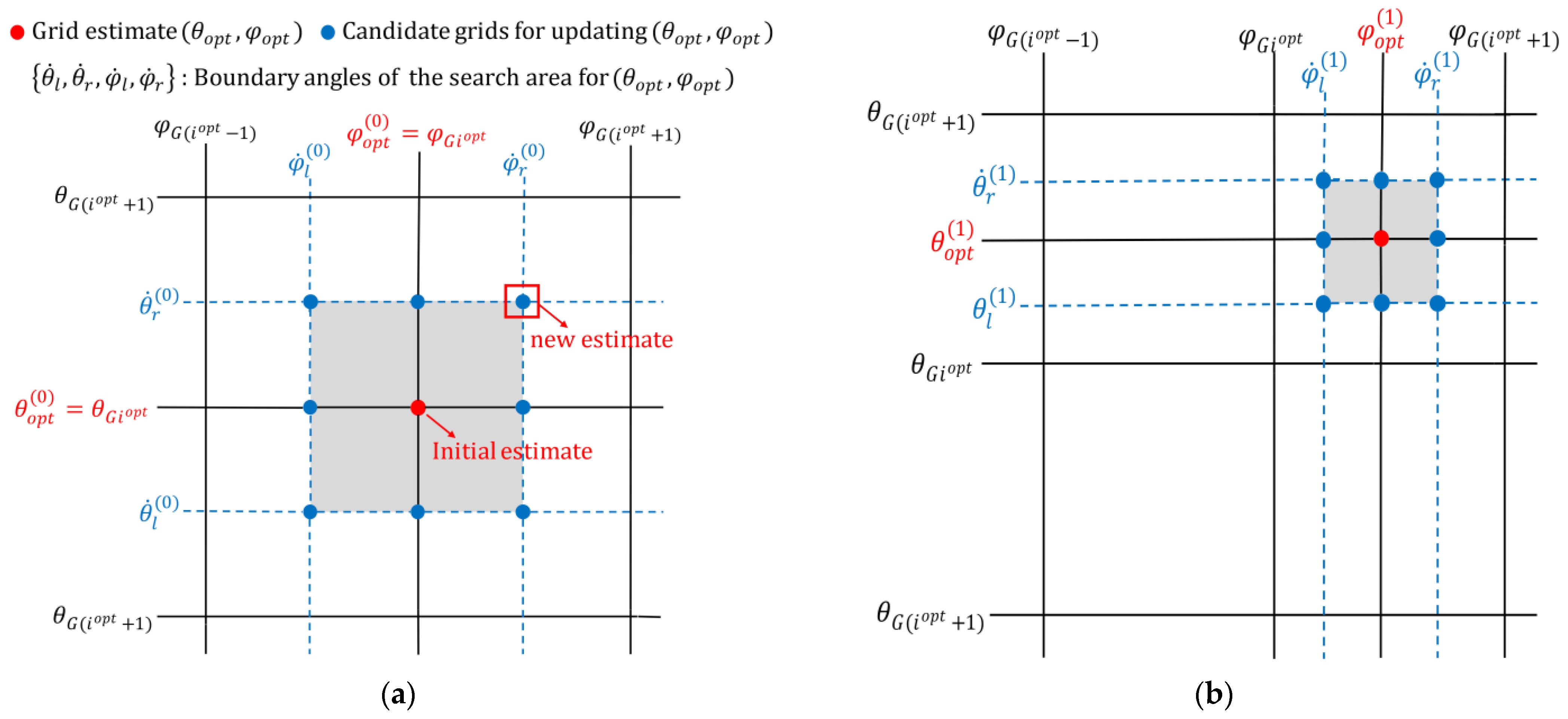
A dichotomizing method is then presented to solve (16) by iteratively refining $({\theta }_{G{i}^{opt}},{\phi }_{G{i}^{opt}})$ within a bounded area that shrinks with each iteration. More specifically, at each iteration, the range of $({\theta }_{G{i}^{opt}},{\phi }_{G{i}^{opt}})$ in (16) is limited to an area centered around the previous estimate. As the iteration proceeds, this area is continuously zoomed in, and more accurate estimates are obtained within this area. The processing is as follows:

(1) Initialization: Set the solution of (15) as the initial estimate for (16), i.e.,

$$({\theta }_o^{(0)},{\phi }_o^{(0)})=({\theta }_{G{i}^{opt}},{\phi }_{G{i}^{opt}}),$$

(17)

where the superscript (n) represents the nth iteration. The initial search ranges for elevation and azimuth angles are $[{\dot{\theta }}_l^{(0)},{\dot{\theta }}_r^{(0)}]$ and $[{\dot{\phi }}_l^{(0)},{\dot{\phi }}_r^{(0)}]$, respectively, where ${\dot{\theta }}_l^{(0)}=\left({\theta }_{G{i}^{opt}}+{\theta }_{G(i^{opt}-1)}\right)/2$, ${\dot{\theta }}_r^{(0)}=\left({\theta }_{G{i}^{opt}}+{\theta }_{G(i^{opt}+1)}\right)/2$, ${\dot{\phi }}_l^{(0)}=\left({\phi }_{G{i}^{opt}}+{\phi }_{G(i^{opt}-1)}\right)/2$, and ${\dot{\phi }}_r^{(0)}=\left({\phi }_{G{i}^{opt}}+{\phi }_{G(i^{opt}+1)}\right)/2$. Based on this, a candidate grid set is defined below, as shown in Figure 2.

$$\begin{array}{ll}{\Theta }_c^{(0)}& =\left\{({\theta }_o^{(0)},{\phi }_o^{(0)}),({\theta }_o^{(0)},{\dot{\phi }}_l^{(0)}),({\theta }_o^{(0)},{\dot{\phi }}_r^{(0)}),({\dot{\theta }}_l^{(0)},{\phi }_o^{(0)}),({\dot{\theta }}_r^{(0)},{\phi }_o^{(0)}),\right.\\ & \left.({\dot{\theta }}_l^{(0)},{\dot{\phi }}_l^{(0)}),({\dot{\theta }}_r^{(0)},{\dot{\phi }}_l^{(0)}),({\dot{\theta }}_l^{(0)},{\dot{\phi }}_r^{(0)}),({\dot{\theta }}_r^{(0)},{\dot{\phi }}_r^{(0)})\right\}.\end{array}$$

(18)

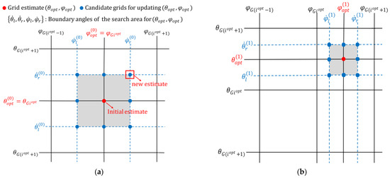
Figure 2. Diagram of the dichotomizing method: (a) initialization; (b) the first iteration.

(2) The nth iteration: Obtain the updated estimate by identifying the grid point that maximizes the cost function in (16) among ${\Theta }_c^{(n-1)}$, as given by:

$$\{{\theta }_o^{(n)},{\phi }_o^{(n)}\}=\underset{{\Theta }_{G{i}^{opt}}\in {\Theta }_c^{(n-1)}}{\arg \max }f({\Theta }_{G{i}^{opt}}).$$

(19)

After obtaining $({\theta }_o^{(n)},{\phi }_o^{(n)})$, the elevation range and azimuth range are updated. The new elevation bounds are given by:

$$\begin{array}{ccc}\begin{array}{l}\mathrm{if} {\theta }_o^{(n)}={\dot{\theta }}_l^{(n-1)}:\\ \mathrm{if} {\theta }_o^{(n)}={\dot{\theta }}_o^{(n-1)}:\\ \mathrm{if} {\theta }_o^{(n)}={\dot{\theta }}_r^{(n-1)}:\end{array}& \begin{array}{l}{\dot{\theta }}_l^{(n)}={\dot{\theta }}_l^{(n-1)}+\left({\dot{\theta }}_l^{(n-1)}-{\theta }_o^{(n-1)}\right)/2,\\ {\dot{\theta }}_l^{(n)}=\left({\dot{\theta }}_l^{(n-1)}+{\theta }_o^{(n-1)}\right)/2,\\ {\dot{\theta }}_l^{(n)}=\left({\dot{\theta }}_r^{(n-1)}+{\theta }_o^{(n-1)}\right)/2,\end{array}& \begin{array}{l}{\dot{\theta }}_r^{(n)}=\left({\dot{\theta }}_l^{(n-1)}+{\theta }_o^{(n-1)}\right)/2\\ {\dot{\theta }}_r^{(n)}=\left({\dot{\theta }}_r^{(n-1)}+{\theta }_o^{(n-1)}\right)/2\\ {\dot{\theta }}_r^{(n)}=\left({\dot{\theta }}_r^{(n-1)}+{\theta }_o^{(n-1)}\right)/2\end{array}\end{array}$$

(20)

and the new azimuth bounds are given by:

$$\begin{array}{ccc}\begin{array}{l}\mathrm{if} {\phi }_o^{(n)}={\dot{\phi }}_l^{(n-1)}:\\ \mathrm{if} {\phi }_o^{(n)}={\phi }_o^{(n-1)}:\\ \mathrm{if} {\phi }_o^{(n)}={\dot{\phi }}_r^{(n-1)}:\end{array}& \begin{array}{l}{\dot{\phi }}_l^{(n)}={\dot{\phi }}_l^{(n-1)}+\left({\dot{\phi }}_l^{(n-1)}-{\phi }_o^{(n-1)}\right)/2,\\ {\dot{\phi }}_l^{(n)}=\left({\dot{\phi }}_l^{(n-1)}+{\phi }_o^{(n-1)}\right)/2,\\ {\dot{\phi }}_l^{(n)}=\left({\dot{\phi }}_r^{(n-1)}+{\phi }_o^{(n-1)}\right)/2,\end{array}& \begin{array}{l}{\dot{\phi }}_r^{(n)}=\left({\dot{\phi }}_l^{(n-1)}+{\phi }_o^{(n-1)}\right)/2\\ {\dot{\phi }}_r^{(n)}=\left({\dot{\phi }}_r^{(n-1)}+{\phi }_o^{(n-1)}\right)/2\\ {\dot{\phi }}_r^{(n)}={\dot{\phi }}_r^{(n-1)}+\left({\dot{\phi }}_r^{(n-1)}-{\phi }_o^{(n-1)}\right)/2\end{array}\end{array}$$

(21)

Then, a new candidate set ${\Theta }_c^{(n)}$ is obtained according to (18) for the next iteration.

The number of iterations required by the dichotomizing method depends on the initial angular grid interval (GI) and the desired computational accuracy of the $({\theta }_o,{\phi }_o)$ estimate. Assuming a GI of $2^{\circ }$ is used for grid discretization in both azimuth and elevation ranges, 15 iterations are sufficient to achieve a computational accuracy of $2^{\circ }/2^{15}<{0.0001}^{\circ }$, which is sufficient for the $({\theta }_o,{\phi }_o)$ estimate. In the numerical simulations, we set 15 iterations for the dichotomizing method.

The overall process of estimating a potential active grid is outlined in Table 1. In practice, the estimated $({\theta }_o,{\phi }_o)$ is used to replace the initial predefined grid $({\theta }_{G{i}^{opt}},{\phi }_{G{i}^{opt}})$, when $({\theta }_o,{\phi }_o)$ is added to the active set ${\Theta }_{active}$.

Table 1. Active grid selection and optimization processes.

Input: ${\Theta }_G$ and ${\mathcal{I}}_{active}$.

1 Perform active grid selection:   Obtain $({\theta }_{G{i}^{opt}},{\phi }_{G{i}^{opt}})$, $i^{opt}\notin {\mathcal{I}}_{active}$, by solving (15) using ${\Theta }_G$. 2 Perform grid optimization using the dichotomizing method:   (1) set $({\theta }_o^{(0)},{\phi }_o^{(0)})=({\theta }_{G{i}^{opt}},{\phi }_{G{i}^{opt}})$, and obtain ${\Theta }_c^{(0)}$ according to (18);   (2) for n = 1 to 15:     update $({\theta }_o^{(n)},{\phi }_o^{(n)})$ by solving (19) using ${\Theta }_c^{(n-1)}$;     update ${\Theta }_c^{(n)}$ using (18), (20), and (21).    end

Output: $({\theta }_o^{(n)},{\phi }_o^{(n)})$ and $i^{opt}$.

3.2.3. Estimation of Noise Precision $\beta$

The previous process assumes that the noise precision $\beta$ is known, which may not be true in many practical situations. Typically, $\beta$ can be estimated by differentiating the log-marginal likelihood function $\mathcal{L}(\alpha ,{\Theta }_{active},\beta )$ with respect to $\beta$ and equating the derivative to zero [18,19,21]. Here, we use the maximum likelihood noise update rule [22,23] to obtain a more accurate $\beta$ estimate:

$$\beta ={\displaystyle \frac{M-\tilde{K}}{\mathrm{tr}\left[\left(I_M-A({\Theta }_{active})A^{†}({\Theta }_{active})\right){\widehat{R}}_Y\right]}},$$

(22)

where ${\widehat{R}}_Y=Y{Y}^H/L$, and $\tilde{K}$ is the number of active grids.

3.2.4. The Iterative Procedure of Array Manifold Matrix Learning

This subsection details the iterative procedure of the array manifold matrix learning-based parameter estimation. In this procedure, signal parameters (i.e., the active set, the signal precision) and the noise precision are updated alternatingly and iteratively. The fundamental content of the array manifold matrix learning process is provided below.

Remember, the grid indexes of active grids are collected in ${\mathcal{I}}_{active}$; the active set is ${\Theta }_{active}={\{({\tilde{\theta }}_k,{\tilde{\phi }}_k)\}}_{k=1}^{\tilde{K}}$, as expressed in (8); the corresponding signal precisions are ${\left\{{\tilde{\alpha }}_k\right\}}_{k=1}^{\tilde{K}}$; and ${(\cdot )}_{-k}$ represents the bracketed term with the factor related to $({\tilde{\theta }}_k,{\tilde{\phi }}_k)$ removed.

(1) Initialization: The noise precision $\beta$ is set to ${10}^3$. The active set ${\Theta }_{active}$ starts empty. From this, the matrix $C={\beta }^{-1}{I}_M$ in (10). Following Table 1, a predefined grid of index $i^{opt(0)}$ is selected, optimized to $({\theta }_o^{(0)},{\phi }_o^{(0)})$, and serves as the initial active set, i.e., ${\Theta }_{active}^{(0)}=({\theta }_o^{(0)},{\phi }_o^{(0)})$. In other words, the first element in the active set is $({\tilde{\theta }}_1^{(0)},{\tilde{\phi }}_1^{(0)})=({\theta }_o^{(0)},{\phi }_o^{(0)})$, and $\tilde{K}=1$. It is worth mentioning that the superscript (n) in this subsection means the nth iteration. The identified active grid index $i^{opt(0)}$ is added to the set ${\mathcal{I}}_{active}$. The corresponding signal precision ${\alpha }_{i^{opt(0)}}$ is obtained from (14), yielding the initial precision vector ${\tilde{\alpha }}^{(0)}={\alpha }_{i^{opt(0)}}$. The posterior signal mean ${\{{\mu }^{(0)}(t)\}}_{t=1}^L$ and covariance ${\Sigma }^{(0)}$ are then computed using (9). After this, ${\beta }^{(0)}$ is estimated using (22).

(2) The nth iteration mainly involves six steps:

Step 1: Determine a new $({\theta }_o^{(n)},{\phi }_o^{(n)})$ outside of ${\Theta }_{active}^{(n-1)}$.

A new $({\theta }_o^{(n)},{\phi }_o^{(n)})$ of grid index $i^{opt(n)}$ is estimated following Table 1, and the corresponding precision ${\alpha }_{i^{opt(n)}}$ is computed using (14).

Step 2: Evaluate the log-marginal likelihood increments associated with the new $({\theta }_o^{(n)},{\phi }_o^{(n)})$ and the active grids in ${\Theta }_{active}^{(n-1)}$, respectively.

For the new $({\theta }_o^{(n)},{\phi }_o^{(n)})$, the log-marginal likelihood increment is computed by:

$$\Delta {\mathcal{l}}_o^{(n)}=\mathcal{l}({\alpha }_{i^{opt(n)}},{\theta }_o^{(n)},{\phi }_o^{(n)})$$

(23)

For each active grid in ${\Theta }_{active}^{(n-1)}$, update parameters $p_{{\tilde{\theta }}_k^{(n-1)},{\tilde{\phi }}_k^{(n-1)}}^{(n)}$ and $s_{{\tilde{\theta }}_k^{(n-1)},{\tilde{\phi }}_k^{(n-1)}}^{(n)}$ by [17]:

$$\left\{\begin{array}{l}{p}_{{\tilde{\theta }}_k^{(n-1)},{\tilde{\phi }}_k^{(n-1)}}^{(n)}={\displaystyle \frac{{\displaystyle {\sum }_{t=1}^L{\left|{\mu }_k^{(n-1)}(t)\right|}^2}}{L{\left({\Sigma }_{k,k}^{(n-1)}\right)}^2}}\\ s_{{\tilde{\theta }}_k^{(n-1)},{\tilde{\phi }}_k^{(n-1)}}^{(n)}={\displaystyle \frac{1}{{\Sigma }_{k,k}^{(n-1)}}}-{\tilde{\alpha }}_k^{(n-1)}\end{array}\right., k=1,\cdots ,\tilde{K}$$

(24)

where $({\tilde{\theta }}_k^{(n-1)},{\tilde{\phi }}_k^{(n-1)})$ is the kth active grid, ${\tilde{\alpha }}_k^{(n-1)}$ is the corresponding precision, ${\mu }_k^{(n-1)}(t)$ is the kth element in ${\mu }^{(n-1)}(t)$, and ${\Sigma }_{k,k}^{(n-1)}$ is the (k,k)th element in ${\Sigma }^{(n-1)}$. With the updated $p_{{\tilde{\theta }}_k,{\tilde{\phi }}_k}^{(n)}$ and $s_{{\tilde{\theta }}_k,{\tilde{\phi }}_k}^{(n)}$, the new precision parameter can be obtained using (14), recorded as ${\tilde{\alpha }}_k^{new}$. The log-marginal likelihood increment caused by ${\tilde{\alpha }}_k^{new}$ can be computed as:

$$\Delta {\mathcal{l}}_k^{(n)}=\left\{\begin{array}{ll}\Delta {\mathcal{l}}_k^{\prime (n)}=-\mathcal{l}({\tilde{\alpha }}_k^{(n-1)},{\tilde{\theta }}_k^{(n-1)},{\tilde{\phi }}_k^{(n-1)}),& \mathrm{if} p_{{\tilde{\theta }}_k^{(n-1)},{\tilde{\phi }}_k^{(n-1)}}^{(n)}\le s_{{\tilde{\theta }}_k^{(n-1)},{\tilde{\phi }}_k^{(n-1)}}^{(n)}\\ \begin{array}{ll}\Delta {\mathcal{l}}_r^{″(n)}& =\mathcal{l}({\tilde{\alpha }}_k^{new},{\tilde{\theta }}_k^{(n-1)},{\tilde{\phi }}_k^{(n-1)})\\ & -\mathcal{l}({\tilde{\alpha }}_k^{(n-1)},{\tilde{\theta }}_k^{(n-1)},{\tilde{\phi }}_k^{(n-1)}),\end{array}& \mathrm{if} p_{{\tilde{\theta }}_k^{(n-1)},{\tilde{\phi }}_k^{(n-1)}}^{(n)}>s_{{\tilde{\theta }}_k^{(n-1)},{\tilde{\phi }}_k^{(n-1)}}^{(n)}\end{array}\right.$$

(25)

Step 3: Update ${\Theta }_{active}^{(n)}$ with the grid bringing the maximum log-marginal likelihood increment.

Compare the log-marginal likelihood increments $\Delta {\mathcal{l}}_o^{(n)}$ and ${\{\Delta {\mathcal{l}}_k^{(n)}\}}_{k=1}^{\tilde{K}}$. If the maximum one is $\Delta {\mathcal{l}}_o^{(n)}$, then $\tilde{K}=\tilde{K}+1$, and execute the addition operation. Specifically, the estimated $({\theta }_o^{(n)},{\phi }_o^{(n)})$ is added to ${\Theta }_{active}^{(n-1)}$ and becomes the $\tilde{K}\mathrm{th}$ active grid, yielding the new ${\Theta }_{active}^{(n)}=\{{\Theta }_{active}^{(n-1)},({\theta }_o^{(n)},{\phi }_o^{(n)})\}$. Similarly, the precision vector is updated as ${\tilde{\alpha }}^{(n)}={[{({\tilde{\alpha }}^{(n-1)})}^T,{\alpha }_{i^{opt(n)}}]}^T$. The set of active grid indexes ${\mathcal{I}}_{active}$ is updated by adding $i^{opt(n)}$ to it.

If the maximum log-marginal likelihood increment is $\Delta {\mathcal{l}}_k^{(n)}=\Delta {\mathcal{l}}_k^{″(n)}$, then $\tilde{K}=\tilde{K}-1$, and execute the deletion operation. Specifically, the corresponding $({\tilde{\theta }}_k^{(n-1)},{\tilde{\phi }}_k^{(n-1)})$ and ${\tilde{\alpha }}_k^{(n-1)}$ are deleted from ${\Theta }_{ative}^{(n-1)}$ and ${\tilde{\alpha }}^{(n-1)}$, respectively, yielding the new ${\Theta }_{active}^{(n)}={({\Theta }_{active}^{(n-1)})}_{-k}$ and ${\tilde{\alpha }}^{(n)}={({\tilde{\alpha }}^{(n-1)})}_{-k}$. Then, the grid index of $({\tilde{\theta }}_k^{(n-1)},{\tilde{\phi }}_k^{(n-1)})$ is removed from ${\mathcal{I}}_{active}$.

If the maximum log-marginal likelihood increment is $\Delta {\mathcal{l}}_k^{(n)}=\Delta {\mathcal{l}}_k^{\prime (n)}$, the corresponding ${\tilde{\alpha }}_k^{(n-1)}$ is replaced by the re-estimated ${\tilde{\alpha }}_k^{new}$ without any grid change, i.e., ${\Theta }_{active}^{(n)}={\Theta }_{active}^{(n-1)}$, and ${\tilde{\alpha }}^{(n)}={\tilde{\alpha }}^{(n-1)}$ with ${\tilde{\alpha }}_k^{(n-1)}={\tilde{\alpha }}_k^{new}$.

Step 4: Sequentially update the active grids in the new ${\Theta }_{active}^{(n)}$ to improve the estimation accuracy.

Let $K^{\prime }=\tilde{K}$ record the total number of active grids to be updated, as $\tilde{K}$ may change during this processing. The re-estimated value of the kth active grid $({\tilde{\theta }}_k^{(n)},{\tilde{\phi }}_k^{(n)})$, denoted by $({\tilde{\theta }}_k^{new},{\tilde{\phi }}_k^{new})$, $k=1,\cdots ,K^{\prime }$, is obtained though the grid optimization in Table 1. In this process, $({\tilde{\theta }}_k^{(n)},{\tilde{\phi }}_k^{(n)})$ is temporarily removed from ${\Theta }_{active}^{(n)}$ with $\tilde{K}=\tilde{K}-1$, serving as the initial estimate in grid optimization. After re-estimation, if $p_{{\tilde{\theta }}_k^{new},{\tilde{\phi }}_k^{new}}>s_{{\tilde{\theta }}_k^{new},{\tilde{\phi }}_k^{new}}$, $({\tilde{\theta }}_k^{new},{\tilde{\phi }}_k^{new})$ is accepted, replacing $({\tilde{\theta }}_k^{(n)},{\tilde{\phi }}_k^{(n)})$, and is added back to ${\Theta }_{active}^{(n)}$ with $\tilde{K}=\tilde{K}+1$. Otherwise, if $p_{{\tilde{\theta }}_k^{new},{\tilde{\phi }}_k^{new}}\le s_{{\tilde{\theta }}_k^{new},{\tilde{\phi }}_k^{new}}$, $({\tilde{\theta }}_k^{new},{\tilde{\phi }}_k^{new})$ is discarded, and $({\tilde{\theta }}_k^{(n)},{\tilde{\phi }}_k^{(n)})$ is permanently removed from ${\Theta }_{active}^{(n)}$. Then, the grid index of $({\tilde{\theta }}_k^{(n)},{\tilde{\phi }}_k^{(n)})$ is removed from ${\mathcal{I}}_{active}$.

Step 5: Calculate the posterior signal statistics ${\mu }^{(n)}(t)$ and ${\Sigma }^{(n)}$ using (9). The signal estimate is obtained by ${\tilde{X}}^{(n)}=[{\mu }^{(n)}(1),\cdots ,{\mu }^{(n)}(L)]$.

Step 6: Update the noise precision ${\beta }^{(n)}$ using (22).

(3) Iteration termination conditions: The iteration will terminate when the iteration number n reaches the maximum number, which is defined as $MaxIter$, or when the following convergence criterion is met:

$$\mathrm{size}({\tilde{X}}^{(n)})=\mathrm{size}({\tilde{X}}^{(n-1)}) \mathrm{and} {\displaystyle \frac{{‖{\tilde{X}}^{(n)}-{\tilde{X}}^{(n-1)}‖}_F^2}{{‖{\tilde{X}}^{(n-1)}‖}_F^2}}\le \tau ,$$

(26)

where $\tau$ is the convergence threshold. The summary of the proposed DOA estimator using manifold matrix learning is given in Table 2.

Table 2. Proposed fast 2D DOA estimator using array manifold matrix learning.

Input: $Y$, $MaxIter$ and $\tau$. Initialization: Set $\beta ={10}^3$.   Obtain $({\theta }_o^{(0)},{\phi }_o^{(0)})$ and $i^{opt(0)}$ following Table 1, and then compute ${\alpha }_{i^{opt(0)}}$ using (14).   Obtain ${\Theta }_{active}^{(0)}=({\theta }_o^{(0)},{\phi }_o^{(0)})$, ${\tilde{\alpha }}^{(0)}={\alpha }_{i^{opt(0)}}$, $\tilde{K}=1$, and add $i^{opt(0)}$ to ${\mathcal{I}}_{ative}$.   Compute ${\beta }^{(0)}$ using (22), and set $n=1$.

While $n\le MaxIter$ and the convergence condition (26) not satisfied do   (a) Determine a new $({\theta }_o^{(n)},{\phi }_o^{(n)})$ outside of ${\Theta }_{active}^{(n-1)}$:    (a1) obtain $({\theta }_o^{(n)},{\phi }_o^{(n)})$ and its grid index $i^{opt(n)}$, according to Table 1;    (a2) compute ${\tilde{\alpha }}_{i^{opt(n)}}$ using (14).   (b) Evaluate $\Delta {\mathcal{l}}_o^{(n)}$ and $\Delta {\mathcal{l}}_k^{(n)}$, $k=1,\cdots ,\tilde{K}$:    (b1) for $({\theta }_o^{(n)},{\phi }_o^{(n)})$, compute $\Delta {\mathcal{l}}_o^{(n)}$ using (23);    (b2) for $({\tilde{\theta }}_k^{(n-1)},{\tilde{\phi }}_k^{(n-1)})$ in ${\Theta }_{active}^{(n-1)}$, update $s_{{\tilde{\theta }}_k^{(n-1)},{\tilde{\phi }}_k^{(n-1)}}^{(n)}$ and $p_{{\tilde{\theta }}_k^{(n-1)},{\tilde{\phi }}_k^{(n-1)}}^{(n)}$ using (24);    (b3) compute ${\tilde{\alpha }}_k^{new}$ using (14), if $p_{{\tilde{\theta }}_k^{(n-1)},{\tilde{\phi }}_k^{(n-1)}}^{(n)}>s_{{\tilde{\theta }}_k^{(n-1)},{\tilde{\phi }}_k^{(n-1)}}^{(n)}$;    (b4) compute $\Delta {\mathcal{l}}_k^{(n)}$ using (25).   (c) Update ${\Theta }_{active}^{(n)}$:    (c1) compare ${\{\Delta {\mathcal{l}}_o^{(n)},\Delta {\mathcal{l}}_k^{(n)}\}}_{k=1}^{\tilde{K}}$ and find the maximum one;    (c2) if it is $\Delta {\mathcal{l}}_o^{(n)}$, ${\Theta }_{active}^{(n)}=\{{\Theta }_{active}^{(n-1)},({\theta }_o^{(n)},{\phi }_o^{(n)})\}$, ${\tilde{\alpha }}^{(n)}={[{({\tilde{\alpha }}^{(n-1)})}^T,{\tilde{\alpha }}_{i^{opt(n)}}]}^T$,      add $i^{opt(n)}$ to ${\mathcal{I}}_{active}$, and $\tilde{K}=\tilde{K}+1$;    (c3) if it is $\Delta {\mathcal{l}}_k^{(n)}=\Delta {\mathcal{l}}_k^{\prime (n)}$, ${\Theta }_{active}^{(n)}={({\Theta }_{active}^{(n-1)})}_{-k}$, ${\tilde{\alpha }}^{(n)}={({\tilde{\alpha }}^{(n-1)})}_{-k}$,      remove the grid index of $({\tilde{\theta }}_k^{(n-1)},{\tilde{\phi }}_k^{(n-1)})$ from ${\mathcal{I}}_{active}$, and $\tilde{K}=\tilde{K}-1$;    (c4) if it is $\Delta {\mathcal{l}}_k^{(n)}=\Delta {\mathcal{l}}_k^{″(n)}$, ${\Theta }_{active}^{(n)}={\Theta }_{active}^{(n-1)}$, and ${\tilde{\alpha }}^{(n)}={\tilde{\alpha }}^{(n-1)}$ with ${\tilde{\alpha }}_k^{(n-1)}={\tilde{\alpha }}_k^{new}$.   (d) Sequentially update the active grids in ${\Theta }_{active}^{(n)}$:      (d1) $K^{\prime }=\tilde{K}$;    for k = 1 to $\tilde{K}$      (d2) remove $({\tilde{\theta }}_k^{(n)},{\tilde{\phi }}_k^{(n)})$ from ${\Theta }_{active}^{(n)}$, and $\tilde{K}=\tilde{K}-1$;      (d3) obtain $({\tilde{\theta }}_k^{new},{\tilde{\phi }}_k^{new})$ by grid optimization in Table 1, using $({\tilde{\theta }}_k^{(n)},{\tilde{\phi }}_k^{(n)})$ as the initial estimate;      (d4) if $p_{{\tilde{\theta }}_k^{new},{\tilde{\phi }}_k^{new}}>s_{{\tilde{\theta }}_k^{new},{\tilde{\phi }}_k^{new}}$, add $({\tilde{\theta }}_k^{(n)},{\tilde{\phi }}_k^{(n)})=({\tilde{\theta }}_k^{new},{\tilde{\phi }}_k^{new})$ back to ${\Theta }_{active}^{(n)}$, and $\tilde{K}=\tilde{K}+1$;      (d5) if $p_{{\tilde{\theta }}_k^{new},{\tilde{\phi }}_k^{new}}\le s_{{\tilde{\theta }}_k^{new},{\tilde{\phi }}_k^{new}}$, discard $({\tilde{\theta }}_k^{new},{\tilde{\phi }}_k^{new})$, and remove the grid index of $({\tilde{\theta }}_k^{(n)},{\tilde{\phi }}_k^{(n)})$ from ${\mathcal{I}}_{active}$.    end   (e) Update ${\tilde{X}}^{(n)}$:    (e1) compute ${\{{\mu }^{(n)}(t)\}}_{t=1}^L$ and ${\Sigma }^{(n)}$ using (9);    (e2) obtain ${\tilde{X}}^{(n)}=[{\mu }^{(n)}(1),\cdots ,{\mu }^{(n)}(L)]$.   (f) Update ${\beta }^{(n)}$ using (22).   (g) $n=n+1$. End while

Output: ${\Theta }_{active}^{(n)}$ and ${\tilde{X}}^{(n)}$.

3.2.5. Enhanced-Efficiency Implementation for URAs

When dealing with a URA, the objective function $f({\Theta }_{Gi})$ in the active grid selection Problem (15) can be reformulated in the 2D FFT form, enabling direct application of the 2D zoom-FFT technique [20] to efficiently estimate the active grid.

Consider a URA that comprises $M=M_y\times M_z$ sensors equispaced by $d_y$ in the y direction and $d_z$ in the z direction, as depicted in Figure 1b. The manifold vector of a $({\theta }_{Gi},{\phi }_{Gi})$ can be expressed as a Kronecker product of two components, given by:

$$a({\theta }_{Gi},{\phi }_{Gi})=a(u_i)\otimes a(v_i),$$

(27)

where

$$\left\{\begin{array}{l}a(u_i)={[1,\exp (j2\pi u_i),\cdots ,\exp (j2\pi (M_y-1)u_i)]}^T\\ a(v_i)={[1,\exp (j2\pi v_i),\cdots ,\exp (j2\pi (M_z-1)v_i)]}^T\end{array}\right.,$$

(28)

with $u_i=d_y\sin {\theta }_{Gi}\sin {\phi }_{Gi}/\lambda$ and $v_i=d_z\cos {\theta }_{Gi}/\lambda$, regarded as spatial frequencies.

For a $({\theta }_{Gi},{\phi }_{Gi})$, $i\notin {\mathcal{I}}_{active}$, not in the active set ${\Theta }_{active}$, the corresponding $s_{{\theta }_{Gi},{\phi }_{Gi}}$, as expressed in (12), is $s_{{\theta }_{Gi},{\phi }_{Gi}}=a_i^H{C}_{-i}^{-1}{a}_i=a^H({\theta }_{Gi},{\phi }_{Gi})C^{-1}a({\theta }_{Gi},{\phi }_{Gi})$, where $a_i$ is the compact representation of $a({\theta }_{Gi},{\phi }_{Gi})$, and $C_{-i}=C={\beta }^{-1}{I}_M+A({\Theta }_{active}){\tilde{\Lambda }}^{-1}{A}^H({\Theta }_{active})$. Using (27), $s_{{\theta }_{Gi},{\phi }_{Gi}}$ can be reformulated as:

$$\begin{array}{ll}{s}_{{\theta }_i,{\phi }_i}& =a^H({\theta }_{Gi},{\phi }_{Gi})C^{-1}a({\theta }_{Gi},{\phi }_{Gi})\\ & =\beta a^H({\theta }_i,{\phi }_i)\left(I_M-\beta A({\Theta }_{active})\Sigma A^H({\Theta }_{active})\right)a({\theta }_i,{\phi }_i)\\ & =\beta M-{\beta }^2{‖a^H({\theta }_{Gi},{\phi }_{Gi})A({\Theta }_{active}){\Sigma }^{1/2}‖}_2^2\\ & =\beta M-{\beta }^2{\displaystyle \sum _{k=1}^{\tilde{K}}{\left|a^H(v_i){\mathrm{vec}}^{-1}\left(Z(:,k)\right)a^{\ast }(u_i)\right|}^2},\end{array}$$

(29)

where $C^{-1}=\beta \left(I_M-\beta A({\Theta }_{active})\Sigma A^H({\Theta }_{active})\right)$, $Z=A{\Sigma }^{1/2}$, and $Z(:,k)$ is the kth column vector of $Z$. The similar reformulation is applied to $p_{{\theta }_{Gi},{\phi }_{Gi}}$ in (13), yielding:

$$\begin{array}{ll}{p}_{{\theta }_i,{\phi }_i}& =\left(1/L\right){\displaystyle \sum _{t=1}^L{\left|a^H({\theta }_i,{\phi }_i)C^{-1}y(t)\right|}^2}\\ & =\left({\beta }^2/L\right){\displaystyle \sum _{t=1}^L{\left|a^H({\theta }_i,{\phi }_i)\left(I_M-\beta A({\Theta }_{active})\Sigma A^H({\Theta }_{active})\right)y(t)\right|}^2}\\ & =\left({\beta }^2/L\right){\displaystyle \sum _{t=1}^L{\left|a^H({\theta }_i,{\phi }_i)\left(y(t)-A({\Theta }_{active})\mu (t)\right)\right|}^2}\\ & =\left({\beta }^2/L\right){\displaystyle \sum _{t=1}^L{\left|a^H(v_i){\mathrm{v}\mathrm{e}\mathrm{c}}^{-1}\left(y(t)-A({\Theta }_{active})\mu (t)\right)a^{\ast }(u_i)\right|}^2}.\end{array}$$

(30)

Note that the manifold vector components, $a(v_i)$ and $a(u_i)$, as expressed in (28), have a structural similarity to the FFT basis function. This suggests that both $s_{{\theta }_{Gi},{\phi }_{Gi}}$ and $p_{{\theta }_{Gi},{\phi }_{Gi}}$ manifest a 2D FFT structure. Accordingly, the cost function of the active grid selection Problem (15) can be reformulated in the 2D FFT domain:

$$f({\Theta }_{Gi})={\displaystyle \frac{p_{{\theta }_{Gi},{\phi }_{Gi}}}{s_{{\theta }_{Gi},{\phi }_{Gi}}}}={\displaystyle \frac{\beta {\displaystyle {\sum }_{t=1}^L{\left|a^H(v_i){\mathrm{vec}}^{-1}\left(y(t)-A\mu (t)\right)a^{\ast }(u_i)\right|}^2}}{L\left(M-\beta {\displaystyle {\sum }_{k=1}^{\tilde{K}}{\left|a^H(v_i){\mathrm{vec}}^{-1}\left(Z(:,k)\right)a^{\ast }(u_i)\right|}^2}\right)}}$$

(31)

From this, the 2D zoom-FFT method [20] can be utilized to maximize (31) and obtain the optimal grid solution. In 2D zoom-FFT, the coarse optimal estimate is located and then refined to obtain a more accurate estimate. Compared to the conventional zero-padding 2D FFT, the 2D zoom-FFT requires fewer FFT points to achieve the same resolution, which results in increased computational efficiency.

Assume that an $(N_1\times N_2)$-point 2D zoom-FFT is performed to estimate the optimal solution to the maximization of $f({\Theta }_{Gi})$. First, $p_{{\theta }_{Gi},{\phi }_{Gi}}$ and $s_{{\theta }_{Gi},{\phi }_{Gi}}$ are computed using an $(N_1\times N_2)$-point 2D FFT, and $f({\Theta }_{Gi})$ is obtained as an $(N_1\times N_2)$ matrix. The 2D spatial frequency pair $(v_{i^{opt}},u_{i^{opt}})$ of the maximum value of $f({\Theta }_{Gi})$ is the coarse optimal solution. Subsequently, $(v_{i^{opt}},u_{i^{opt}})$ is iteratively refined via the dichotomizing method introduced in the previous section. Put simply, each refinement iteration re-locates the maximum values of $f({\Theta }_{Gi})$ among the last updated estimate and its neighbor frequence points, which are newly interpolated in the search area. Defining the finally tuned 2D frequency pair by $(v_o,u_o)$, following the previous notation, the optimal grid estimate $({\theta }_o,{\phi }_o)$ can be computed by:

$$\left\{\begin{array}{l}{\theta }_o={\cos }^{-1}\left(v_o\lambda /d_z\right)\\ {\phi }_o={\sin }^{-1}\left(u_o\lambda /\left(d_y\sqrt{1-{\cos }^2{\theta }_o}\right)\right)\end{array}\right.,$$

(32)

where $({\theta }_o,{\phi }_o)$ is accepted if the constraint $p_{{\theta }_o,{\phi }_o}>s_{{\theta }_o,{\phi }_o}$ is satisfied; otherwise, $({\theta }_o,{\phi }_o)$ is discarded if $p_{{\theta }_o,{\phi }_o}\le s_{{\theta }_o,{\phi }_o}$. It is noteworthy that the active grid selection and optimization processes are simultaneously achieved by maximizing (31) with the 2D zoom-FFT.

Recall the outline of the proposed fast 2D DOA estimator in Table 2. When dealing with a URA, the initialization, step a, and step d need to be modified. Specifically, the active grid estimation based on the criteria presented in Table 1 is replaced by maximizing (31) by the 2D zoom-FFT method, where the optimal grid estimate is obtained using (32).

3.3. Complexity Analysis

The computational complexity of the proposed fast 2D DOA estimator is measured by the number of multiplication operations in a single iteration. The estimator consists of two processes: the grid selection process and the grid optimization process, which are performed in an alternating manner. The grid selection process dominates the complexity due to its grid searching over predefined grids covering a large space, whereas the grid optimization process has negligible complexity as it is confined to a small bounded area around the selected grid. Recall the grid selection problem, as represented in (15). At each iteration, the parameters $p_{{\theta }_{Gi},{\phi }_{Gi}}$ and $s_{{\theta }_{Gi},{\phi }_{Gi}}$ are computed for $Q-\tilde{K}$ candidate grid points ${\{({\theta }_{Gi},{\phi }_{Gi})\}}_{i=1,i\notin {\mathcal{I}}_{active}}^Q$, requiring $\mathcal{O}(\max \{ML(Q-\tilde{K}),M^2(Q-\tilde{K})\})$ complexity, where $M$, $L$, $Q$, and $\tilde{K}$ are the numbers of sensors, snapshots, predefined grid points, and active grids, respectively. Additionally, the posterior estimates of source signals are computed at each iteration, resulting in a complexity of $\mathcal{O}(\max (M{\tilde{K}}^2,M\tilde{K}L))$. Therefore, the computational complexity of the proposed estimator is approximately $\mathcal{O}(\max \{ML(Q-\tilde{K}),M^2(Q-\tilde{K}),M{\tilde{K}}^2,M\tilde{K}L\})$ per iteration.

Regarding the grid-based SR method, whose computational complexity often concentrates on calculating the signal covariance matrix. The computational complexity of the conventional SBL method is $\mathcal{O}(\max (M{Q}^2,MQL))$ per iteration [10]. For the fast SR method SAMV-RELAX [13], its computational complexity depends on the SAMV step, which is $\mathcal{O}(M^{2}Q)$ [12]. Since $\tilde{K}$ increases from zero and retains a small value during estimation, we have $Q\gg \tilde{K}$. Based on this, it can be observed that the proposed DOA estimator has a significantly lower complexity than the conventional SBL method, and a slight decrease in complexity compared to SAMV-RELAX, indicating improved efficiency.

For URAs, the efficiency of the proposed DOA estimator is improved by using the 2D zoom-FFT in active grid estimation compared to the dichotomizing-based solver. This is because the 2D zoom-FFT can require fewer FFT points than the number of predefined grids used by the dichotomizing-based solver, with similar accuracy.

3.4. Correlation to the FAMML Method

This work extends the 1D FAMML method in [17] to 2D DOA estimation and focuses on reducing computational complexity. The crucial task in the extension is to devise an efficient 2D grid refinement to reduce the off-grid errors and thereby achieve high accuracy. A dichotomizing-based grid refinement method, applicable to arbitrary planar arrays, is proposed, which iteratively modifies the coarse grid within a bounded area that shrinks with each iteration. This method directly maximizes the objective function in (16) without relying on derivatives on the objective function, as done in FAMML. FAMML will yield a multivariate equation system, while its root cannot be solved with the bisection method used by FAMML. Moreover, Newton’s method, mentioned in FAMML, requires calculation of partial derivatives of (16), leading to increased computational complexity compared with the dichotomizing method. For 2D DOA estimation with URAs, a 2D zoom-FFT-based grid refinement is developed. This method exploits the Kronecker structure of the manifold vector to formulate the cost function in the 2D FFT domain, as expressed in (31). Based on this, the refined grid can be obtained by the 2D zoom-FFT technique, providing computational efficiency improvements over the dichotomizing-based solver.

4. Simulation Results

In this section, we compare the performance of the proposed fast 2D DOA estimator with two fast SR methods: SAMV-RELAX [13] and FGML [15]. The version of the proposed estimator that uses the dichotomizing method for grid optimization is referred to as Method 1. The URA-tailored variant that uses the 2D zoom-FFT is referred to as Method 2. The simulations are considered as being implemented in an underwater free field. The source velocity is 1500 m/s. Narrowband signals with frequency of 6 kHz and equal power of 0 dB impinge on the planar array. These source signals are located in the far field relative to the planar array. The sample frequency is 30 kHz.

During simulations, two array configurations are considered, a URA and an arbitrary planar array, as shown in Figure 1. The URA, consisting of $M=M_y\times M_z=6\times 4$ sensors with $d_y=d_z=\lambda /2$, is utilized for all four methods to assess their performance. The arbitrary planar array of M sensors is utilized to demonstrate Method 1’s adaptability to different array configurations. Unless otherwise stated, simulation results are obtained from 200 Monte Carlo trials, where $K=4$ uncorrelated narrowband signals with equal power arrival from directions $({\theta }_{S1},{\phi }_{S1})=({80.5}^{\circ },-{37.5}^{\circ })$, $({\theta }_{S2},{\phi }_{S2})=({90.5}^{\circ },-{12.6}^{\circ })$, $({\theta }_{S3},{\phi }_{S3})=({100.5}^{\circ },{8.2}^{\circ })$ and $({\theta }_{S4},{\phi }_{S4})=({110.6}^{\circ },{32.6}^{\circ })$, respectively. The root-mean-square error (RMSE) of DOA estimates is used to evaluate the estimation accuracy of the methods, with the Cramér–Rao bound (CRB) [24] serving as a benchmark. Additionally, the average runtime and resolution performance for both azimuth and elevation angles are evaluated to provide a comprehensive assessment of the methods. All simulations are carried out on a PC with 2.9 GHz CPU and 8 GB RAM.

The parameter settings for the evaluated methods are as follows. A uniform discretization of $2^{\circ }$ is applied to both the azimuth range $[-{90}^{\circ },{90}^{\circ }]$ and the elevation range $[{30}^{\circ },{150}^{\circ }]$. For both proposed methods, the iteration parameters are set to $MaxIter=50$ and $\tau ={10}^{-5}$. In method 1, the iteration number for the dichotomizing-based solver of grid optimization is set to 15. In method 2, a $(32\times 16)$-point 2D zoom-FFT is employed, where the number of iterations for the refinement process is set to 8. For SAMV-RELAX, the parameters are set to $MaxIter=50$ and $\tau ={10}^{-3}$ in the SAMV-step, and $\tau ={10}^{-2}$ in the SAMV-step. Additionally, knowledge of the source number K is required by the SAMV-RELAX and FGML methods. While FGML assumes that K is known, SAMV-RELAX estimates it during the SAMV-step by identifying peaks in the estimated normalized spatial spectrum that surpass a threshold of −5 dB.

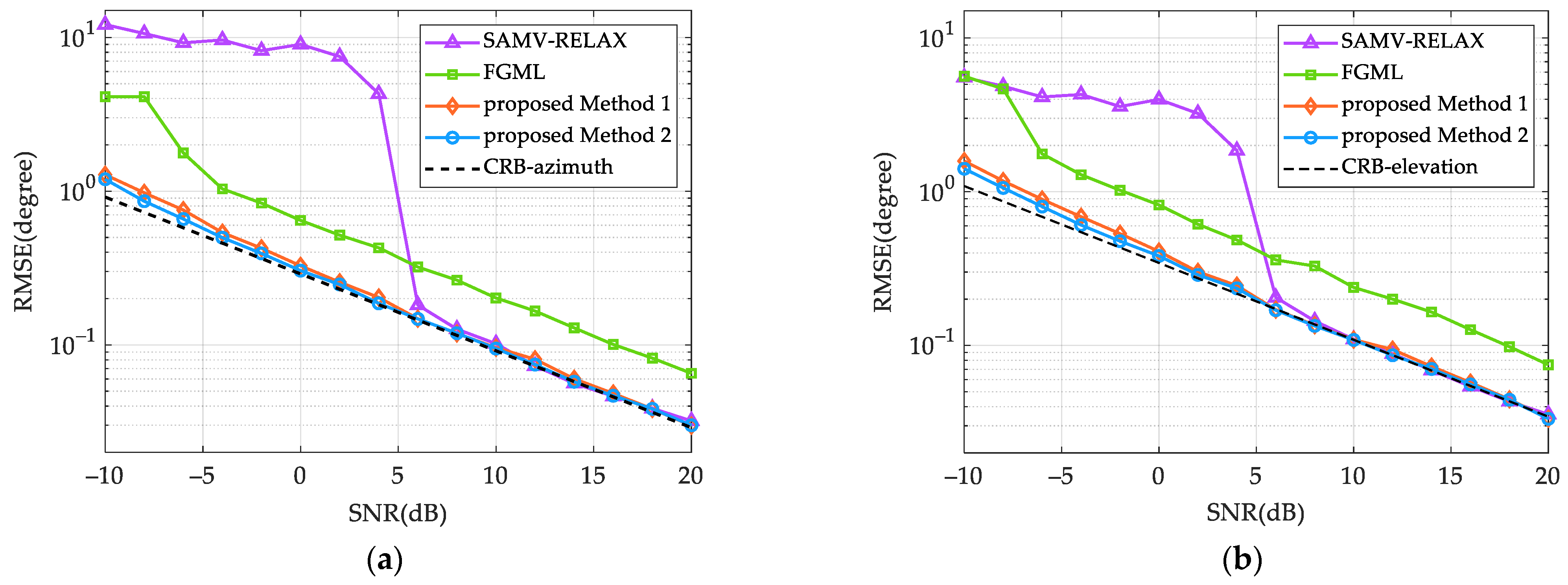
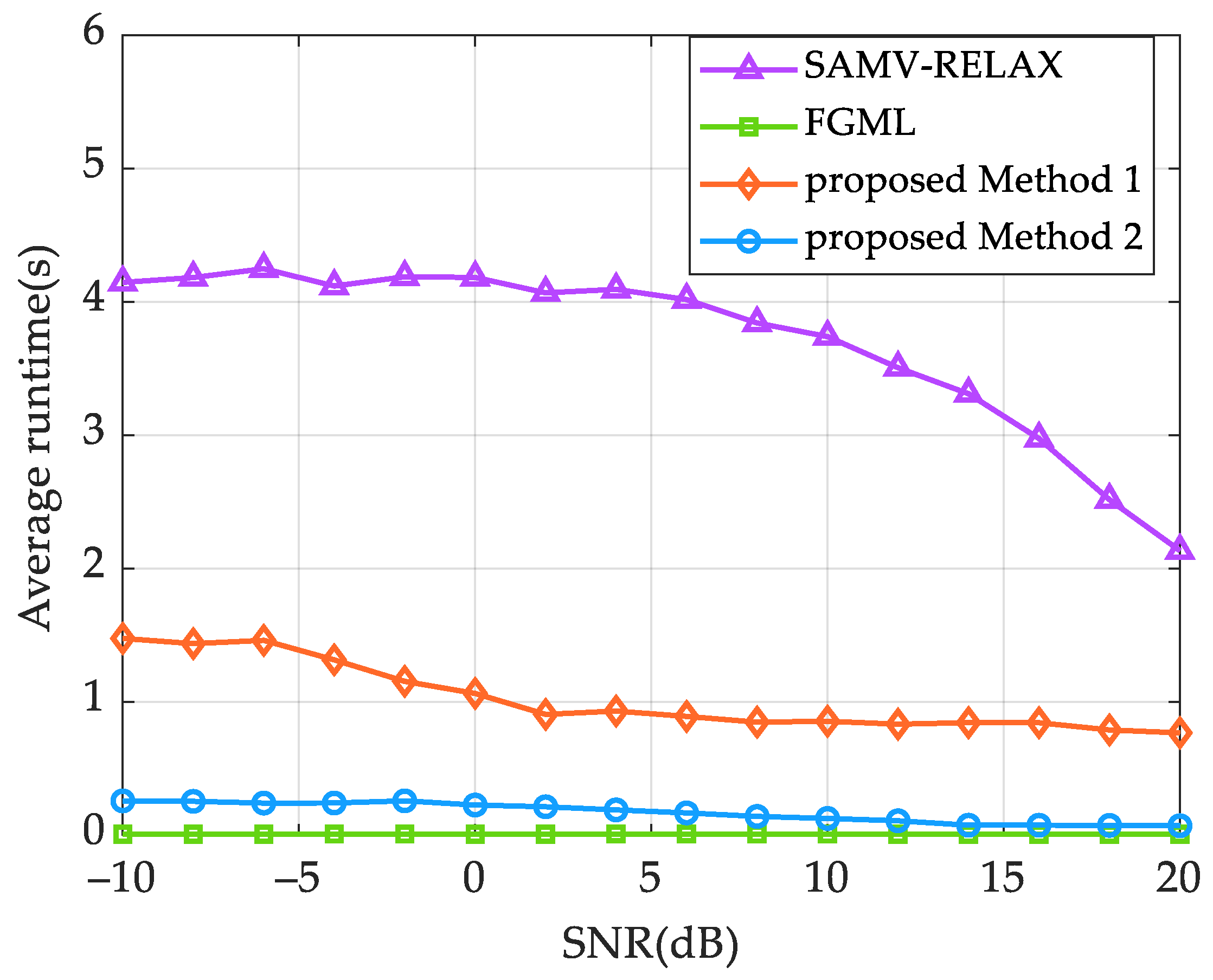
Simulation 1 assesses methods’ estimation performance versus SNR in terms of RMSE and average runtime. The SNR varies from −10 dB to 20 dB, and the snapshots is $L=50$. The URA is utilized for 2D DOA estimation. Figure 3 shows the RMSE results. For each evaluated method, the RMSE performance has a consistent trend across the azimuth and elevation angles. It can be observed that both Method 1 and Method 2 achieve RMSEs close to the CRB across all SNRs, while FGML deviates from the CRB due to insufficient snapshots. Regarding SAMV-RELAX, the RMSEs of this method closely approximate the CRB when $SNR>5 \mathrm{dB}$. However, it becomes considerably larger at lower SNRs. This phenomenon can be attributed to SAMV-RELAX’s tendency to inaccurately estimate the source number K at relatively low SNRs, which negatively impacts the angle estimation accuracy during the RELAX-step. Figure 4 shows the average runtime of the four methods. One can see that SAMV-RELAX has the longest average runtime, while FGML has the shortest. The average runtime of the two proposed methods is positioned between those of FGML and SAMV-RELAX, with Method 2 showing improved efficiency by having a shorter average runtime than Method 1.

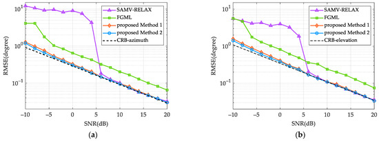
Figure 3. RMSE performance versus SNR, where a URA is utilized, and L is 50: (a) azimuth; (b) elevation.

Figure 4. Average runtime versus SNR, where a URA is utilized, and L is 50.

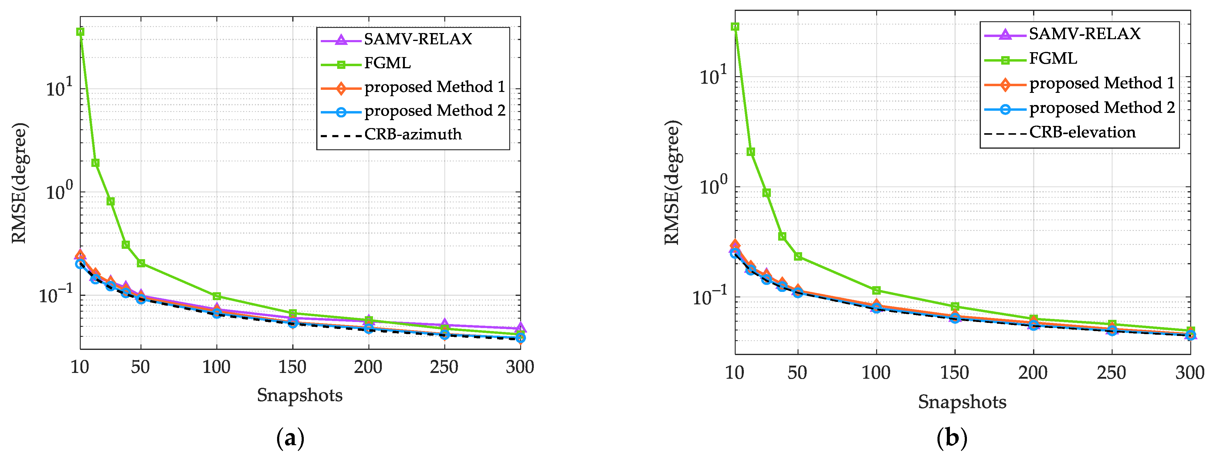
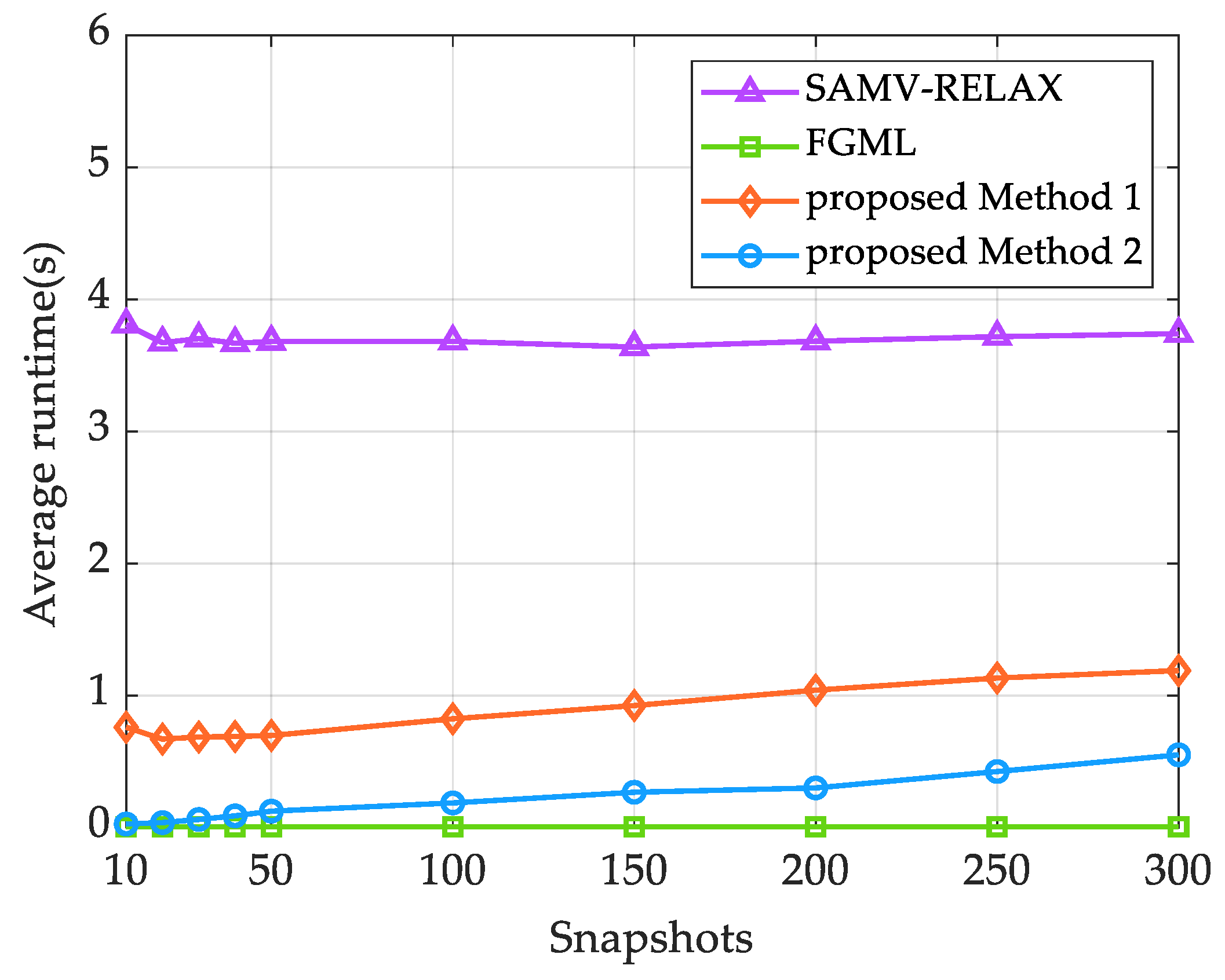
Simulation 2 assesses the estimation performance versus the number of snapshots L, which is swept from 10 to 300. The SNR is fixed at 10 dB with other parameters unchanged. The RMSEs of the four methods are shown in Figure 5. Each method’s RMSE performance has a consistent trend across the azimuth and elevation angles. From Figure 5, the two proposed methods and SAMV-RELAX exhibit similar RMSE performance, closely approaching the CRB across all L. FGML displays a decreasing RMSE trend as L increases, nearing the CRB at relatively large snapshots ($L\ge 200$). The corresponding average runtimes of the four methods are shown in Figure 6. It is seen that FGML is the fastest method, and Method 2 ranks second, followed by Method 1, whereas SAMV-RELAX is the slowest. Although both proposed methods take more time as the number of snapshots grows, Method 2 manages to maintain a runtime of less than one second, demonstrating its enhanced computational efficiency compared to Method 1.

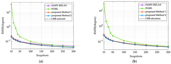
Figure 5. RMSE performance versus snapshots, where a URA is utilized, and SNR is 10 dB: (a) azimuth; (b) elevation.

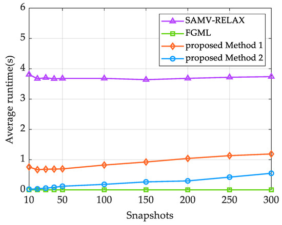
Figure 6. Average runtime versus snapshots, where a URA is utilized, and SNR is 10 dB.

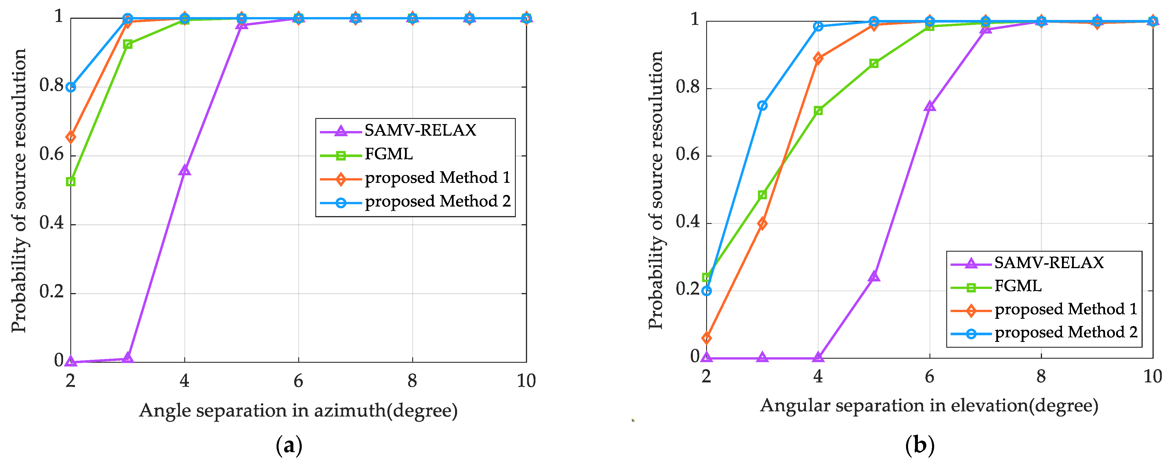
Simulation 3 assesses the angle resolution performance by examining the probability of source resolution [25]. Two equal-power uncorrelated signals are analyzed with the SNR of 10 dB and 50 snapshots. Both the azimuth and elevation resolution of the four methods are compared in this simulation. The angular separation in terms of azimuth and elevation is defined as $\Delta \phi$ and $\Delta \theta$, respectively, with values ranging from $2^{\circ }$ to ${10}^{\circ }$. To model off-grid DOAs, we define an angular deviation as $\delta$, which is randomly selected with a uniform distribution within $[-{0.5}^{\circ },{0.5}^{\circ }]$. In assessing the azimuth resolution capability, the two signals have a common elevation angle of ${90}^{\circ }$ and distinct azimuth angles of $-\Delta \phi /2+{\delta }_{\phi }$ and $\Delta \phi /2+{\delta }_{\phi }$, where ${\delta }_{\phi }$ is the off-grid error of the azimuth. The two signals are said to be resolved in the lth run if [25]:

$${\displaystyle \sum _{i=1}^2\left|{\widehat{\phi }}_i(l)-{\widehat{\phi }}_i\right|}<\left|{\phi }_1-{\phi }_2\right|,$$

(33)

where ${\widehat{\phi }}_i(l)$ is the estimate of the true azimuth ${\phi }_i$ in the $l\mathrm{th}$ run. When assessing elevation resolution capability, the two signals have the same azimuth angle of $0^{\circ }$ and distinct elevation angles of $-\Delta \theta /2+{90}^{\circ }+{\delta }_{\theta }$ and $\Delta \theta /2+{90}^{\circ }+{\delta }_{\theta }$. Similarly, the two signals are said to be resolved if the elevation estimates satisfy (33), in which ${\widehat{\phi }}_i(l)$ and ${\phi }_i$ are replaced by ${\widehat{\theta }}_i(l)$ and ${\theta }_i$, respectively.

Figure 7 shows the simulation results of the probability of source resolution. There is a consistent performance trend for both azimuth and elevation resolution. It is observed that Method 2 exhibits the best resolution performance even in small angular separation scenarios. Although Method 1 has slightly inferior resolution performance compared to Method 2, it outperforms both FGML and SAMV in cases of large angular separation.

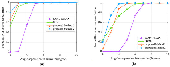
Figure 7. Probability of source resolution versus angular separation, where a URA is utilized, SNR is 10 dB, and L is 50: (a) azimuth; (b) elevation.

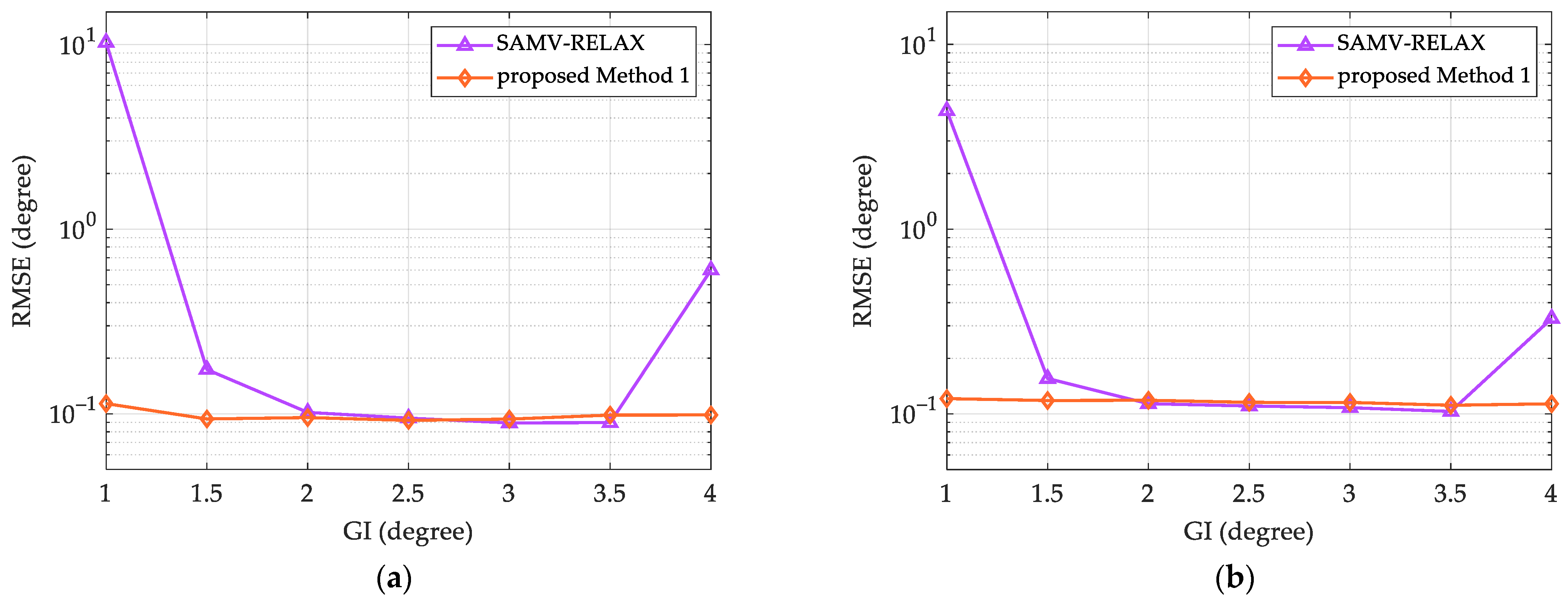
Simulation 4 examines the impact of angular grid interval (GI) on the RMSE performance and average runtime of the methods. In this simulation, GI varies from $1^{\circ }$ to $4^{\circ }$ for grid discretization in both azimuth range and elevation range, with the SNR of 10 dB and 50 snapshots. Set $K=4$ signals with DOAs the same as in Simulation 1. Since Method 2 and FGML do not involve grid discretization, neither are considered.

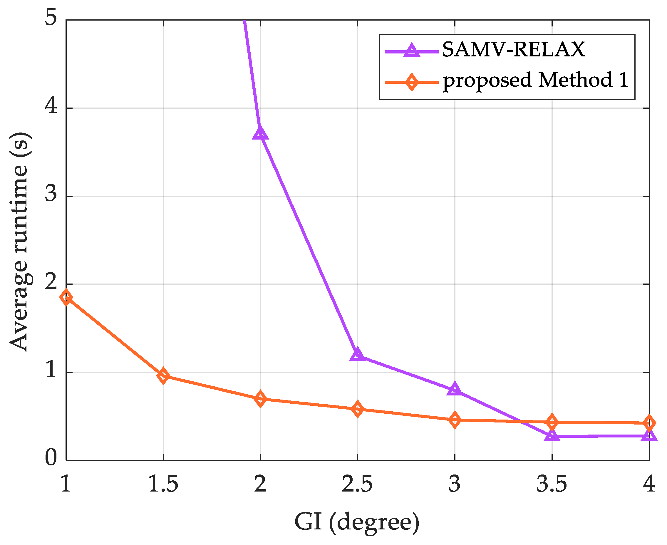
Figure 8 shows the RMSE performance of Method 1 and SAMV-RELAX with respect to GI. Each method exhibits a consistent performance trend for both azimuth and elevation angles. Method 1 has stable RMSE values regardless of GI values, showing robustness to GI. In contrast, SAMV-RELAX exhibits comparable RMSE performance in the GI range of $2^{\circ }$ to ${3.5}^{\circ }$, but it has higher RMSE values at other GI values, indicating reduced accuracy. This accuracy degradation in SAMV-RELAX can be attributed to overestimation of source number, leading to large errors in DOA estimates derived from the RELAX process. Considering the average runtime, Figure 9 shows that both Method 1 and SAMV-RELAX require less time as GI increases. This is because larger GI values lead to fewer grid points, resulting in a reduction in computational workload. When $\mathrm{GI}<{3.5}^{\circ }$, Method 1 spends shorter time than SAMV-RELAX, showing better computational efficiency.

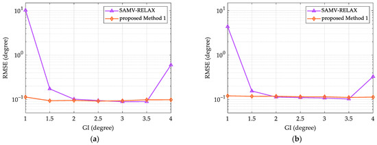
Figure 8. RMSE performance versus GI, where a URA is utilized, SNR is 10 dB, and L is 50: (a) azimuth; (b) elevation.

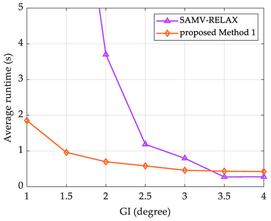
Figure 9. Average runtime versus GI, where a URA is utilized, SNR is 10 dB, and L is 50.

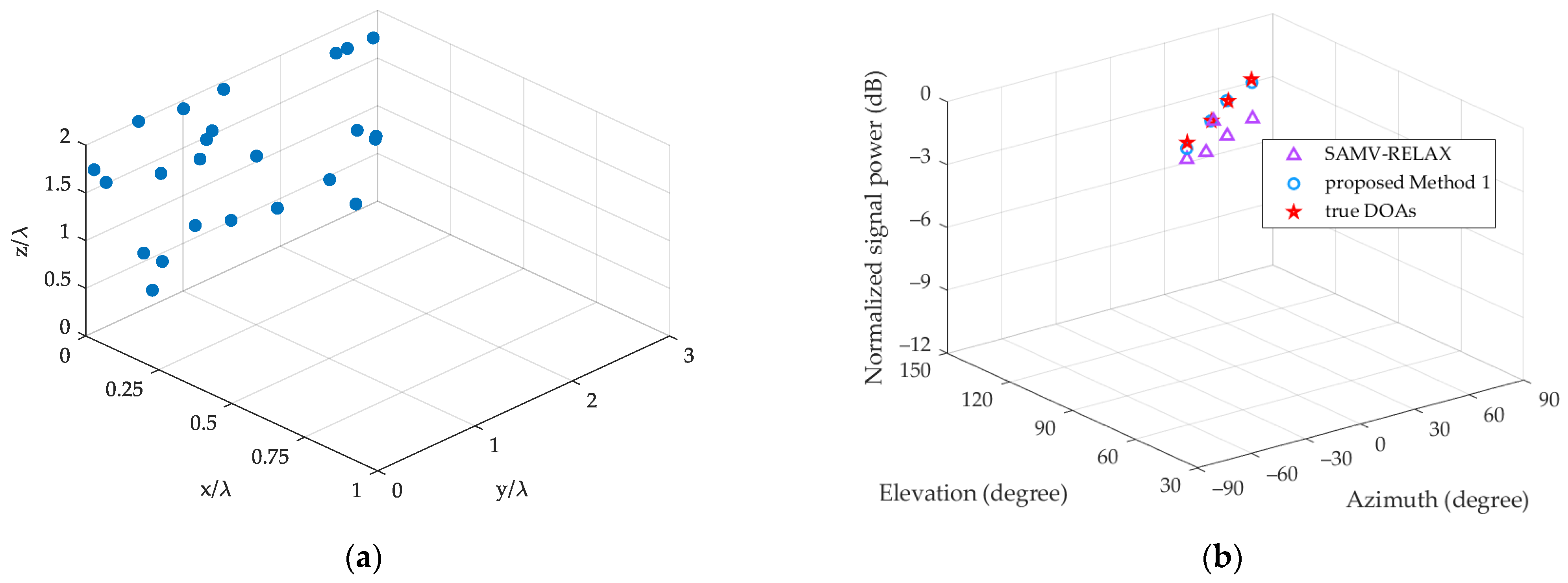
Simulation 5 verifies the adaptability of Method 1 to array configurations. The previous simulations utilize a URA with $M=24$ sensors, while Simulation 5 adopts a non-rectangular array with the same number of sensors to estimate the DOAs of the aforementioned $K=4$ signals from Simulation 1. The locations of array sensors $r_m={[0,y_m,z_m]}^T$, $m=1,\cdots ,M$ are randomly generated within the range of $0\le y_m\le 3\lambda$ and $0\le z_m\le 2\lambda$. Only the proposed Method 1 and SAMV-REALX are available in this arbitrary planar array case, with SNR set to 0 dB and the snapshots to 50. The result of 2D DOA estimation obtained from a random trial is shown in Figure 10. One can see that Method 1 succeeds in localizing all four signals correctly, achieving better estimation than SAMV-RELAX.

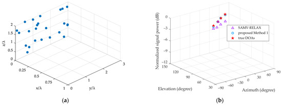
Figure 10. Result of 2D DOA estimation using an arbitrary planar array, where SNR is 0 dB, and L is 50: (a) array configuration; (b) 2D DOA estimates.

5. Conclusions

In this paper, we propose a fast 2D DOA estimator using array manifold matrix learning in the SBL framework. The proposed estimator achieves rapid and accurate 2D DOA estimation through grid selection and optimization processes based on marginal likelihood maximization. In grid optimization, an efficient dichotomizing-based solver is proposed for arbitrary planar arrays, while a 2D zoom-FFT based solver is introduced for URAs with improved computational efficiency. Simulation results demonstrate a superior balance between estimation accuracy and computational efficiency of the proposed DOA estimator compared to state-of-the-art methods. Moreover, the proposed estimator exhibits improvements in resolution probability.

References

- Krim, H.; Viberg, M. Two Decades of Array Signal Processing Research: The Parametric Approach. IEEE Signal Process. Mag. 1996, 13, 67–94. [Google Scholar] [CrossRef]
- Schmidt, R. Multiple Emitter Location and Signal Parameter Estimation. IEEE Trans. Antennas Propag. 1986, 34, 276–280. [Google Scholar] [CrossRef]
- Roy, R.; Kailath, T. ESPRIT-Estimation of Signal Parameters via Rotational Invariance Techniques. IEEE Trans. Acoust. Speech Signal Process. 1989, 37, 984–995. [Google Scholar] [CrossRef]
- Stoica, P.; Nehorai, A. MUSIC, Maximum Likelihood, and Cramer-Rao Bound. IEEE Trans. Acoust. Speech Signal Process. 1989, 37, 720–741. [Google Scholar] [CrossRef]
- Malioutov, D.; Cetin, M.; Willsky, A.S. A Sparse Signal Reconstruction Perspective for Source Localization with Sensor Arrays. IEEE Trans. Signal Process. 2005, 53, 3010–3022. [Google Scholar] [CrossRef]
- Yardibi, T.; Li, J.; Stoica, P.; Xue, M.; Baggeroer, A.B. Source Localization and Sensing: A Nonparametric Iterative Adaptive Approach Based on Weighted Least Squares. IEEE Trans. Aerosp. Electron. Syst. 2010, 46, 425–443. [Google Scholar] [CrossRef]
- Stoica, P.; Babu, P.; Li, J. SPICE: A Sparse Covariance-Based Estimation Method for Array Processing. IEEE Trans. Signal Process. 2011, 59, 629–638. [Google Scholar] [CrossRef]
- Abeida, H.; Zhang, Q.; Li, J.; Merabtine, N. Iterative Sparse Asymptotic Minimum Variance Based Approaches for Array Processing. IEEE Trans. Signal Process. 2013, 61, 933–944. [Google Scholar] [CrossRef]
- Zhu, H.; Leus, G.; Giannakis, G.B. Sparsity-Cognizant Total Least-Squares for Perturbed Compressive Sampling. IEEE Trans. Signal Process. 2011, 59, 2002–2016. [Google Scholar] [CrossRef]
- Yang, Z.; Xie, L.; Zhang, C. Off-Grid Direction of Arrival Estimation Using Sparse Bayesian Inference. IEEE Trans. Signal Process. 2013, 61, 38–43. [Google Scholar] [CrossRef]
- Dai, J.; Bao, X.; Xu, W.; Chang, C. Root Sparse Bayesian Learning for Off-Grid DOA Estimation. IEEE Signal Process. Lett. 2017, 24, 46–50. [Google Scholar] [CrossRef]
- Zhang, Y.; Yang, Y.; Yang, L.; Guo, X. Root Sparse Asymptotic Minimum Variance for Off-Grid Direction-of-Arrival Estimation. Signal Process. 2019, 163, 225–231. [Google Scholar] [CrossRef]
- Park, H.-R.; Li, J. Efficient Sparse Parameter Estimation Based Methods for Two-Dimensional DOA Estimation of Coherent Signals. IET Signal Process. 2020, 14, 643–651. [Google Scholar] [CrossRef]
- Li, J.; Zheng, D.; Stoica, P. Angle and Waveform Estimation via RELAX. IEEE Trans. Aerosp. Electron. Syst. 1997, 33, 1077–1087. [Google Scholar] [CrossRef]
- Wu, X.; Zhu, W.-P.; Yan, J. A Fast Gridless Covariance Matrix Reconstruction Method for One- and Two-Dimensional Direction-of-Arrival Estimation. IEEE Sens. J. 2017, 17, 4916–4927. [Google Scholar] [CrossRef]
- Zoltowski, M.D.; Haardt, M.; Mathews, C.P. Closed-Form 2-D Angle Estimation with Rectangular Arrays in Element Space or Beamspace via Unitary ESPRIT. IEEE Trans. Signal Process. 1996, 44, 316–328. [Google Scholar] [CrossRef]
- Mao, Y.; Guo, Q.; Ding, J.; Liu, F.; Yu, Y. Marginal Likelihood Maximization Based Fast Array Manifold Matrix Learning for Direction of Arrival Estimation. IEEE Trans. Signal Process. 2021, 69, 5512–5522. [Google Scholar] [CrossRef]
- Tipping, M.E. Sparse Bayesian Learning and the Relevance Vector Machine. J. Mach. Learn. Res. 2001, 1, 211–244. [Google Scholar]
- Faul, A.; Avenuse, J. Fast Marginal Likelihood Maximisation for Sparse Bayesian Models. In Proceedings of Machine Learning Research; MLResearchPress: Singapore, 2002. [Google Scholar]
- Liu, Z.-S.; Li, J. Implementation of the RELAX Algorithm. IEEE Trans. Aerosp. Electron. Syst. 1998, 34, 657–664. [Google Scholar]
- Wipf, D.P.; Rao, B.D. An Empirical Bayesian Strategy for Solving the Simultaneous Sparse Approximation Problem. IEEE Trans. Signal Process. 2007, 55, 3704–3716. [Google Scholar] [CrossRef]
- Liu, Z.-M.; Huang, Z.-T.; Zhou, Y.-Y. An Efficient Maximum Likelihood Method for Direction-of-Arrival Estimation via Sparse Bayesian Learning. IEEE Trans. Wirel. Commun. 2012, 11, 1–11. [Google Scholar] [CrossRef]
- Gerstoft, P.; Mecklenbräuker, C.F.; Xenaki, A.; Nannuru, S. Multisnapshot Sparse Bayesian Learning for DOA. IEEE Signal Process. Lett. 2016, 23, 1469–1473. [Google Scholar] [CrossRef]
- Dai, X.; Zhang, X.; Wang, Y. Extended DOA-Matrix Method for DOA Estimation via Two Parallel Linear Arrays. IEEE Commun. Lett. 2019, 23, 1981–1984. [Google Scholar] [CrossRef]
- Gershman, A.B. Direction Finding Using Beamspace Root Estimator Banks. IEEE Trans. Signal Process. 1998, 46, 3131–3135. [Google Scholar] [CrossRef]
Disclaimer/Publisher’s Note: The statements, opinions and data contained in all publications are solely those of the individual author(s) and contributor(s) and not of MDPI and/or the editor(s). MDPI and/or the editor(s) disclaim responsibility for any injury to people or property resulting from any ideas, methods, instructions or products referred to in the content. |
© 2024 by the authors. Licensee MDPI, Basel, Switzerland. This article is an open access article distributed under the terms and conditions of the Creative Commons Attribution (CC BY) license (https://creativecommons.org/licenses/by/4.0/).