Abstract
The calibration of 3D cameras is one of the key challenges to successfully measure the nightly 3D flight tracks of bats with thermal cameras. This is relevant around wind turbines to investigate the impact wind farms have on their species. Existing 3D-calibration methods solve the problem of unknown camera position and orientation by using a reference object of known coordinates. While these methods work well for small monitoring volumes, the size of the reference objects (e.g., checkerboard patterns) limits the distance between the two cameras and therefore leads to increased calibration errors when used in large outdoor environments. To address this limitation, we propose a calibration method for tracking flying animals with thermal cameras based on UAV GPS tracks. The tracks can be scaled to the required monitoring volume and accommodate large distances between cameras, which is essential for low-resolution thermal camera setups. We tested our method at two wind farms, conducting 19 manual calibration flights with a consumer UAV, distributing GPS points from 30 to 260 m from the camera system. Using two thermal cameras with a resolution of 640 × 480 pixels and an inter-axial distance of 15 m, we achieved median 3D errors between 0.9 and 3.8 m across different flights. Our method offers the advantage of directly providing GPS coordinates and requires only two UAV flights for cross-validation of the 3D errors.
1. Introduction
The climate targets, together with the rising demand for clean energy, necessitate more than double the wind energy capacity in the European Union by 2030 as communicated in the European Wind Power Action Plan published by the European Commission [1]. Despite their positive effects on the reduction of human carbon dioxide emissions, wind turbines pose a threat to the bat population because of the turning rotor [2,3,4]. Bats either get hit or suffer from barotrauma due to the pressure changes induced by the rotor blades [5]. It is suspected that bats are potentially attracted by the turbines [6] due to mating behavior [7], foraging [8] and the advantages of high trees [9], but may also avoid them in other cases, which may lead to habitat loss [10]. To understand these effects, many authors in the field use or suggest the use of thermal imaging [11,12,13,14,15,16]. Especially, the extraction of the 3D flight tracks can support in-depth analysis of their nightly flying behavior, including flight direction, speed and height. While methods exist to track bats acoustically and visually in limited spaces [17,18,19,20], extracting 3D flight tracks of bats in large outdoor environments remains a challenge. To extract the 3D flight tracks of bats, a minimum of two thermal cameras with known intrinsic (focal length, optical center and lens distortion) and extrinsic parameters (positions and orientations) have to be installed and the same individual has to be identified in both cameras simultaneously. Accurate 3D reconstruction requires precise measurement of the extrinsic parameters, which is challenging to achieve directly [21]. For this reason, indirect 3D-calibration methods have been developed to solve this by using reference structures with known dimensions.
While the majority of these methods are designed for small, indoor applications and high-resolution visual cameras, only a minority are designed for large outdoor environments or bat measurement. To the best of our knowledge, there is no applicable 3D-calibration method that fits the task of an accurate 3D reconstruction of bat flight tracks using thermal cameras for the large measurement volume of a wind turbine. The main contribution of this paper is a 3D-calibration method using an UAV GPS flight track as the calibration object, which is optimized for low-resolution thermal cameras and large outdoor environments in the dimensions of a wind turbine. The method was tested at two wind farms in Germany, resulting in over 26 h of animal tracks over a time span of 6 months, which will be the subject of a future publication.
2. Related Work
To position this study within existing methods, in this section, we identify the research gaps and the contributions of our work more deeply. A well-known method by [22] uses a checkerboard as a reference structure for 3D calibration. The knowledge about the relative position of the corner points in 3D as well as their location in both images help to recover the pose of the cameras. This method is widely used for stereo camera calibration in general [23,24,25], in the context of bat flight track detection by [26] (limited to small-scale wind turbines), and for bird and bat detection by [27,28,29]. However, all of these applications use a small inter-axial camera distance. But for low-resolution thermal cameras and large-wind-turbine-scale scene sizes, an inter-axial distance of several meters is mandatory to achieve reasonable 3D errors ([30] and Section 3.1). This necessitates a larger calibration object to more appropriately cover the measurement volume [31], which is impractical to achieve with a checkerboard pattern [32], as it must be moved to various angles and distances to be visible to both cameras. To address this problem [33], further developed a method from [34], which is able to perform a 3D calibration without a dedicated calibration object, but still relies on 2D point correspondences visible from both cameras. They use the 8-point algorithm [35] and apply sparse bundle adjustment by [36]. This method is dependent on well-distributed and clearly defined point correspondences in the images, which is a difficult task if the wind turbine is the only object in the scene. Additionally, the final point cloud is scaled using a known distance within the scene to resolve the scale ambiguity [35], which makes it prone to errors due to the limited accuracy of this distance.
Further, all of the above methods rely on a 2D re-projection error for the 3D calibration. By optimizing the 2D re-projection error, the perspective ambiguity [35] is not accounted for, which means that small errors in the intrinsic matrices can propagate to large errors in the reconstructed 3D coordinates. Additionally, the re-projection error is not a direct measure of the final 3D error in meters and makes it difficult to estimate the reliability of the resulting flight tracks. Moreover, the final 3D calibration derived by the mentioned methods is given in one of the camera coordinate systems where the transformation to the geographical coordinate system (WGS 84 or UTM) is not necessarily known and can therefore be challenging.
An experimental comparison between the method from [33,34] and the proposed method was conducted by the authors and can be found in [37]. It shows that the proposed method produces more accurate and stable results. More 3D-calibration methods for cameras with large inter-axial distances can be found by expanding the research to non-thermal cameras [38,39,40,41]. All the methods are compared in Table 1, listing features which are critical to detect nightly flying bats around wind turbines.

Table 1.
Comparison of 3D-calibration methods for large outdoor environments. Cells are colored green if they are necessary or advantageous for the purpose of nightly 3D bat track detection around wind turbines.
In comparison to related work, our method uses thermal cameras and a calibration object of proper size and attributes that can be flexibly distributed in the open space to fit the task of an accurate 3D calibration for tracking bats in the large measurement volume of a wind turbine. Further, no method directly optimizes the 3D errors, which makes our method less susceptible to errors in the intrinsic matrices by not ignoring the depth dimension. Plus, by performing a second drone flight, it allows for direct cross-validation in metric units to estimate the reliability of the resulting flight tracks. Further contributions of our method are:
- The calibration process takes at least two drone flights of a few minutes at the site and can, therefore, be practically used as a mobile setup at different outdoor environments.
- The method is not dependent on any other real-world objects (and knowledge about their dimensions) apart from the drone GPS data and is, therefore, not susceptible to any further errors from coordinate system transformations based on known landmarks.
- The method allows for large base distances, making it especially useful for low-resolution cameras outdoors.
- The 3D points are directly given in geographic coordinates (WGS 84). They can be directly projected to metric UTM coordinates (using the Python module utm [42]) and shifted to the turbine origin, making it possible to calculate the geographic direction, distance to the turbine, flight height and speed of the detected animals. Another advantage of geographic coordinates is that measurements from other camera setups at different positions can be related to each other.
3. Materials and Methods
The following sections contain all the necessary steps to fulfill the objective of operationalizing the UAV flight track as the calibration object in order to accurately sense bats in 3D. A schematic of the steps necessary to measure bats with thermal cameras in 3D is given in Figure 1. Prerequisites are two synchronized cameras with an appropriate inter-axial distance (Section 3.1) which stay in fixed positions during the experiment. To obtain a 3D calibration, a UAV flight (red) is performed with the goal of distributing UAV GPS points in the measurement volume as evenly as possible. This helps to lower the training data bias and can be achieved, e.g., by following a three-dimensional raster pattern at a constant speed. To independently evaluate the 3D error, a second UAV flight (blue) is 3D-reconstructed by using the 3D calibration of the first flight (red) and then compared to the UAV GPS points of the second flight (blue). A cross-validation is possible by interchanging the datasets. Finally, with the same camera setup and the known calibration, bats (or any other flying object) can be 3D-tracked. In this publication, we focus on the 3D camera calibration, reconstruction and error evaluation, not on 2D methods for detecting the points and not on methods to extract single flight tracks from 3D point clouds.
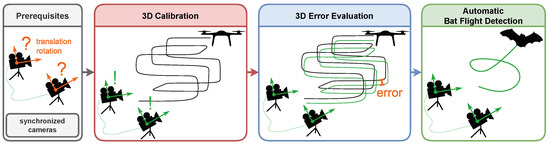
Figure 1.
The automatic bat flight track detection needs two synchronized cameras, one UAV flight to calculate a 3D calibration, a second one to cross-validate the 3D errors and some flying bats to reconstruct their flight tracks.
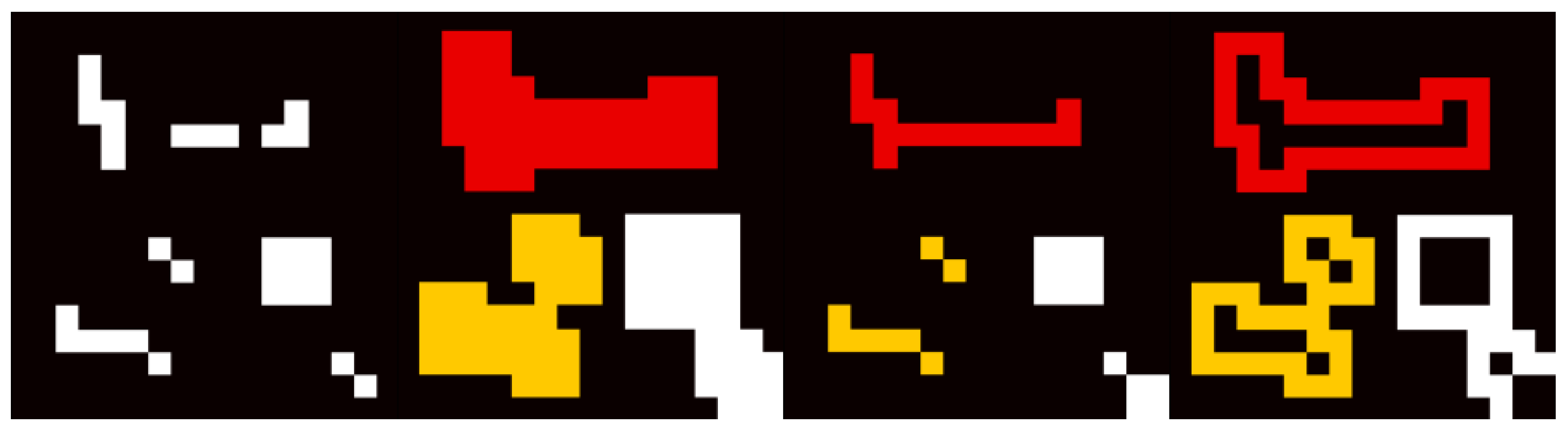
Figure 2 shows a software flowchart of the methods used to achieve each step shown in the schematic in Figure 1. The methods are written in Python and are provided at [43], including all data to reproduce the plots in the results section.
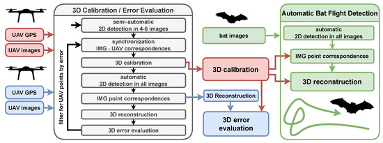
Figure 2.
Main steps for 3D calibration and automatic 3D bat flight track detection. The gray boxes contain all software steps for a 3D calibration. The red boxes represent the data from a drone flight for 3D calibration, the blue boxes another drone flight for 3D error evaluation and the green boxes a bat flight for its 3D reconstruction.
For both UAV flights (red and blue in Figure 1 and Figure 2), the UAV points in both cameras have to be synchronized to the UAV GPS points. We present a method for performing this semi-automatically (Section 3.4): After manually identifying a small set of UAV points in both images (about 4–6 distinct points spread across the whole volume), a preliminary synchronization can be derived. This allows for a preliminary 3D calibration (Section 3.2) using those 4–6 points. Meanwhile, automated machine vision algorithms including background subtraction are used to iterate over the images to find all potential UAV points in the images (Section 3.5). The preliminary calibration is then used to correspond the 2D coordinates of the UAV in both images by epipolar constraints (Section 3.6) and also sort out points without a corresponding partner in the second image. Those corresponding pairs of 2D points are then 3D-reconstructed and by using the initial synchronization the reconstructed points can be compared to the UAV GPS points, which is defined as the 3D error (Section 3.3). In the next step, the 3D error is used to threshold outliers which are likely non-UAV points (like volant animals flying through the scene while performing the UAV flight). At this point, the time synchronization and 3D calibration are still based on the small set of initially identified points, so the next step is to perform an updated fine synchronization and final 3D calibration with the entire set of corresponding 2D-3D points of the UAV. The quality of the final 3D calibration of the first UAV flight is analyzed by the 3D error (Section 3.3) of the second UAV flight. So the 3D calibration of the first flight (red) is used to 3D-reconstruct points from the second flight (blue) which are then compared to the UAV GPS points of the second flight. As long as the cameras stay in their position, the camera setup can be used to automatically detect bats (green). The image-processing methods as well as the steps for corresponding the 2D points are the same, except that the final 3D calibration from above is used to achieve correspondence between the image points and 3D-reconstruct the flight tracks of bats.
3.1. Hardware and Spatial Arrangement
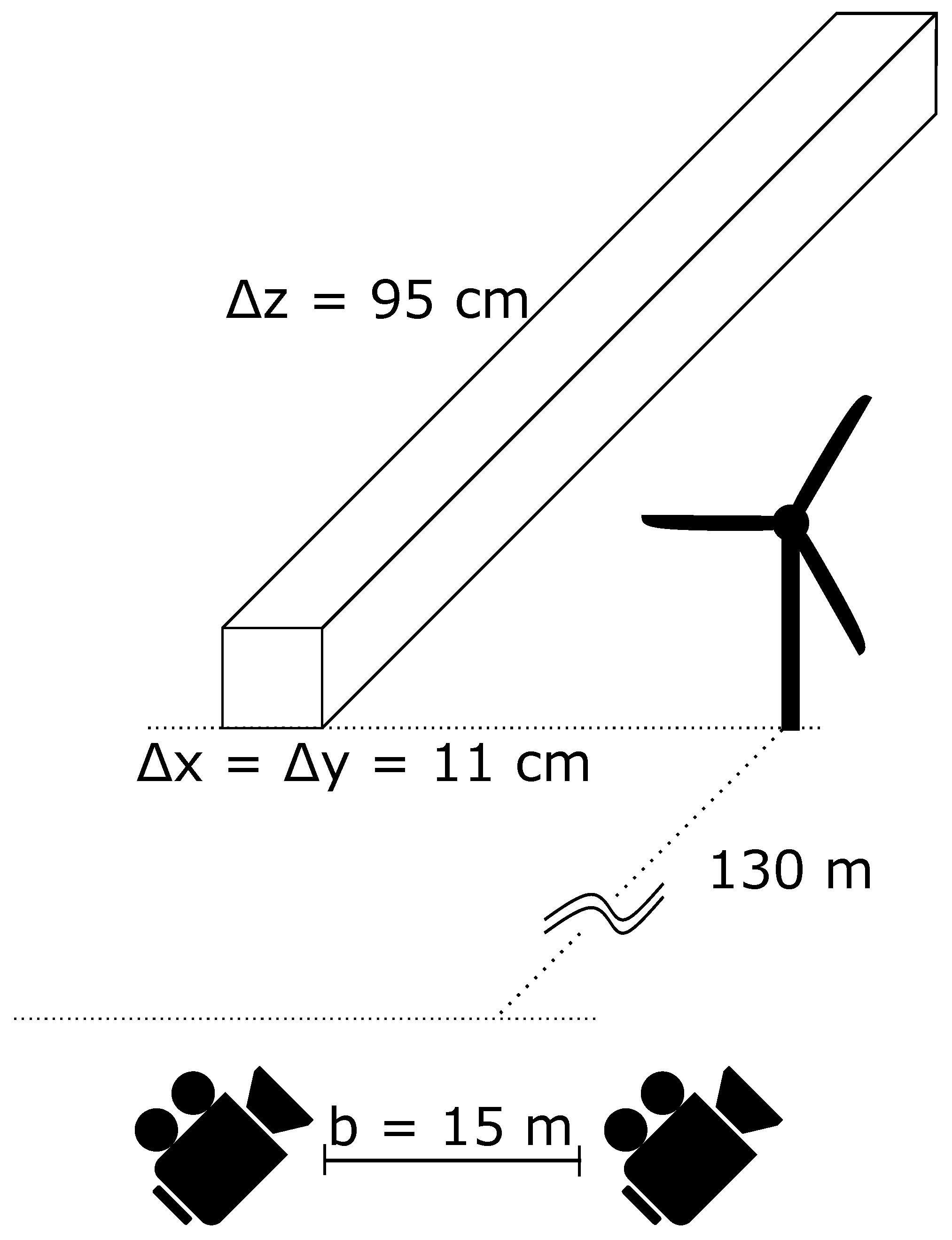
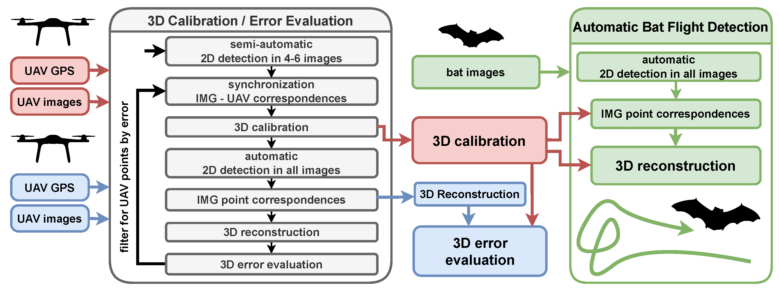
For the 3D system, we used two time-synchronized thermal cameras (Cameras VarioCAM HDx head 600 from Infratec, Germany, Dresden) with 640 × 480 pixels and a horizontal angle of view (=HFOV) of 30°. For the single camera calibration, we calculated the intrinsic matrices and the distortion matrices according to the specification sheet from the manufacturer. More information on the single camera calibration can be found in Appendix B. Due to project restrictions, we placed the cameras approximately 130 m from the wind turbine. In addition, we decided to limit the maximum projected voxel sizes to 1 m at this distance in order to keep the final 3D errors low. Based on these inputs and according to Figure 3, we decided on a camera inter-axial distance of 15 m.
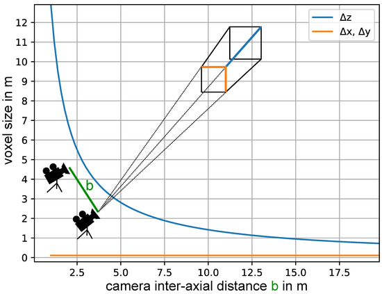
Figure 3.
Projected voxel size in 130 m: and are the projected voxel lengths in the image plane, is the voxel length in the depth direction, b is the camera inter-axial distance, the focal length is 20 mm and the sensor pixel size is 17 μm. The derivation can be found in Appendix A.
The cameras were manually aligned to the wind turbine and not further moved during the measurements. The positioning of the cameras on the met mast in front of the turbine for the Kuchalb location in Germany can be seen in Figure 4.
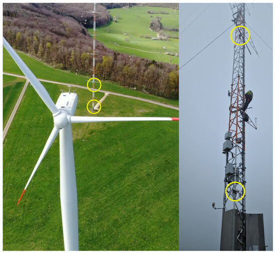
Figure 4.
Positioning of the cameras (yellow circles) on the met mast in front of the turbine for the Kuchalb location in Germany. The camera base distance is 15 m and the distance to the turbine is about 130 m.
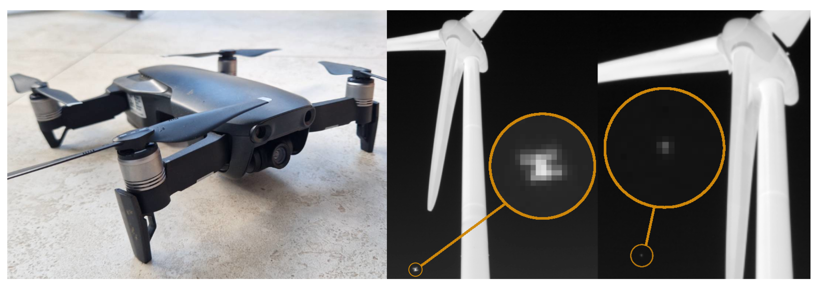
For the calibration flights, we used a Mavic 2 consumer UAV from DJI, Shenzhen, Guangdong, China (Figure 5) with GPS accuracies taken from the data sheet vertically of ±0.1 m (visual positioning) and ±0.5 m (GPS/GLONSASS positioning) and horizontally of ±0.3 m (visual positioning) ±1.5 m (GPS/GLONSASS positioning). We further attached a heat pad to it in order to obtain a more distinct thermal center, which helped in the 2D detection pipeline.

Figure 5.
Mavic 2 drone (left) seen from one Infratec Camera in a distance of 36 m (middle) and 174 m (right).
3.2. 3D Calibration and 3D Reconstruction
For the 3D (extrinsic) calibration, it is required that we have a set of known 2D-3D point correspondences of the UAV for each camera. The 3D calibration is then used to determine the translation vector and the rotation matrix with respect to each camera coordinate system separately. This problem is known as the perspective-n-point problem or camera pose estimation. It was further developed from the 3-point method [44] to an n-point method [45] and since 2020 there exists an efficient solution by [46] implemented in OpenCV 4.5.5.62 by using the function solvePnP with the flag SOLVEPNP_SQPNP. SQPnP minimizes the 3D error between the left and the right side of Equation (1) for all given 2D-3D point correspondences i.
The image coordinates and on the left side of the equation are normalized by projecting them on the plane where . This can be performed by applying Equation (2) for the pixel coordinates and , where is the intrinsic matrix with and being the focal lengths and , being the optical center of the camera. is a scale parameter chosen to equalize the z-coordinate on both sides of the equation.
A 3D reconstruction in the 3D camera coordinate system is derived by multiplying the observed, normalized image coordinates with the z-coordinate of on the left side of Equation (1). The right side of the equation is the actual i-th UAV point transformed to the 3D camera coordinate system. SQPnP minimizes the accumulated, squared residual between the left and right side. The residual is non-zero because of all the inaccuracies involved in the physical system (GPS accuracy, camera intrinsics, camera resolution, 2D object detection accuracy). By having and for both cameras, it is possible to recover the camera projection matrices and according to Equation (3), which are the quantitative representations of the 3D calibration.
To find the unknown 3D points, triangulation is used with the DLT method implemented in OpenCV (triangulatePoints) and described in [35]. The inputs are , and any set of corresponding 2D pixel coordinates , gathered by the same camera setup. The reconstructed 3D points can be written as:
where m denotes the point set used for reconstruction (corresponding image points) and n denotes the point set used for calibration (corresponding image and UAV points).
3.3. 3D Error
The set of 3D errors are the magnitudes of the difference vectors between the UAV GPS points of the point set m and the corresponding 3D reconstruction based on the image points of the same flight for a calibration based on point set n:
where is the distance between the i-th UAV GPS point and the 3D-reconstructed point.
3.4. Time Synchronization of Camera and Drone Signal
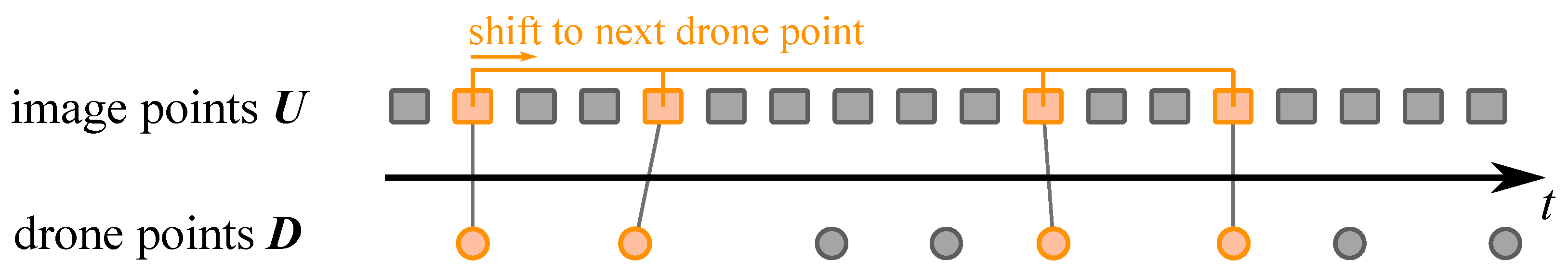
To be able to correspond the 2D image points and and the 3D UAV points from Section 3.2, it is indispensable to time-synchronize the UAV and the camera signals. If the GPS signal of the UAV and the camera signals are assumed to have correct relative timestamps, the problem is reduced to finding the offset between them. This can be achieved by assuming that successful synchronization allows for a meaningful calibration, marked by small errors. Thus, the signals are shifted relative to each other (Figure 6), and the 3D calibration error is repeatedly evaluated to find the minimum:
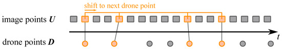
Figure 6.
One time step in the loop to synchronize the UAV GPS points and the camera images. In this example, the UAV was marked in 4 images.
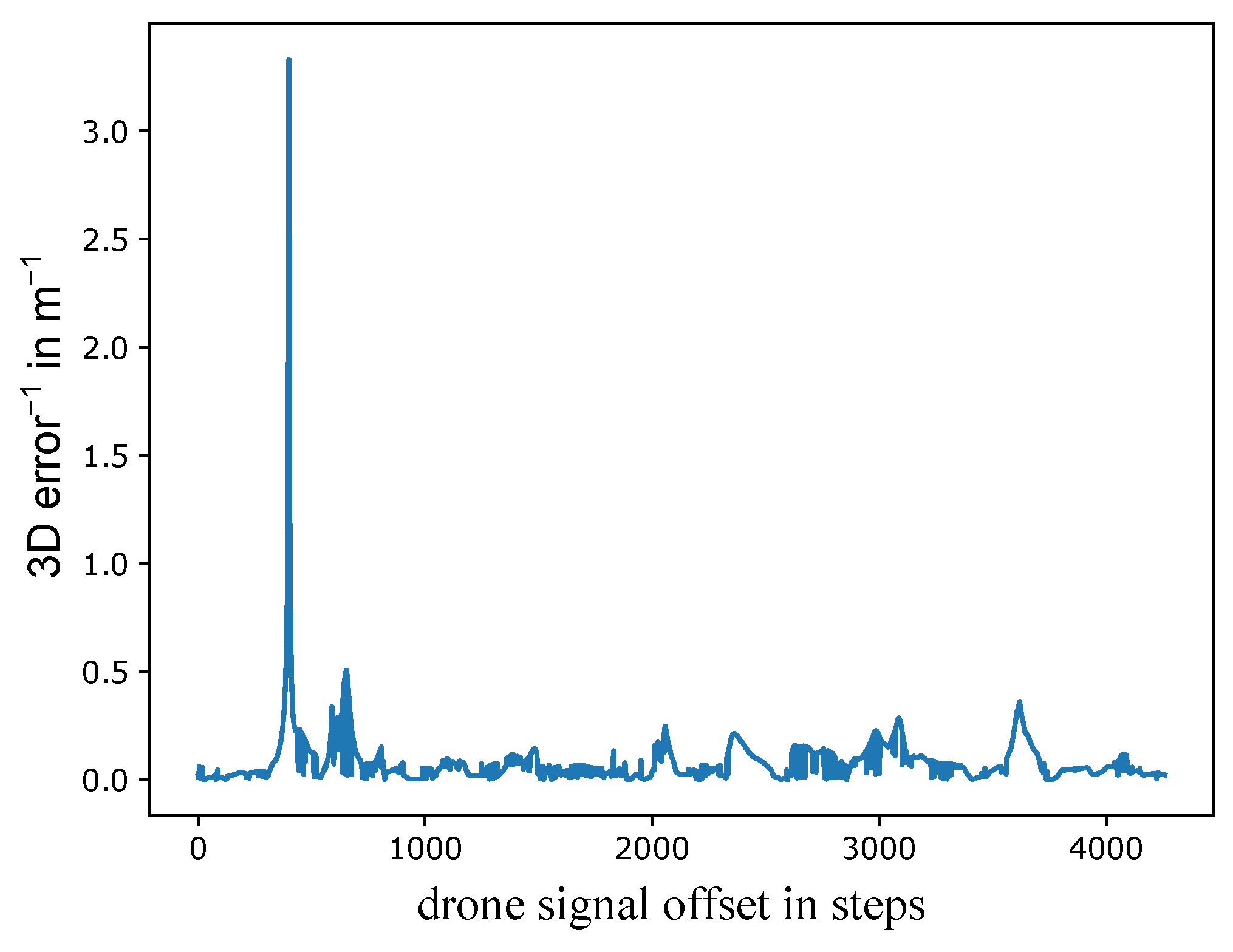
The UAV is identified in a small set of image points in each camera. Four points are usually sufficient to identify a clear 3D error minimum (shown as a maximum in Figure 7). However, using five to six points reduces the likelihood of identifying a false minimum. Using any more points should just verify this solution and increases the manual effort. Finding the minimum error is achieved by a loop over the 3D UAV points according to Figure 6. The first set of 2D image points is aligned to the first UAV point and the closest 3D points at the given time offsets are found. A 3D calibration is performed with k 2D-3D correspondences and the mean 3D error e is saved (Equation (6)).
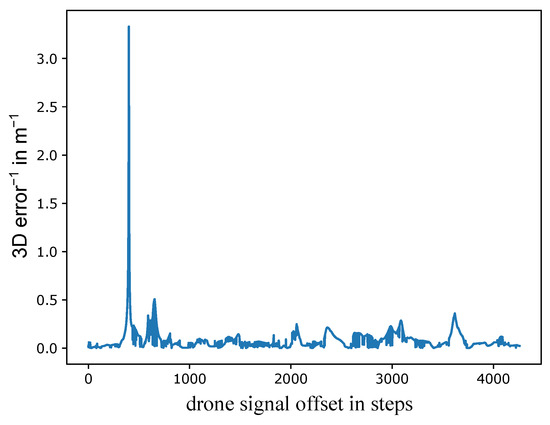
Figure 7.
Reciprocal of mean 3D error over the UAV signal offset for 5 points for an example calibration flight. The correct synchronization can be clearly identified as the maximum.
After the loop has finished, the correct time offset corresponds to the smallest 3D error. This can be seen for flight 1 in Figure 7. The distinct peak shows that a reasonable minimum 3D error was found and a valid synchronization was achieved. The mean 3D error e is plotted as the reciprocal value because it is more convenient to picture the maximum instead of the closest value to zero. By having the correct time offset, all 2D-3D correspondences can be found by their relative timestamps.
3.5. Automated 2D Image Points Detection
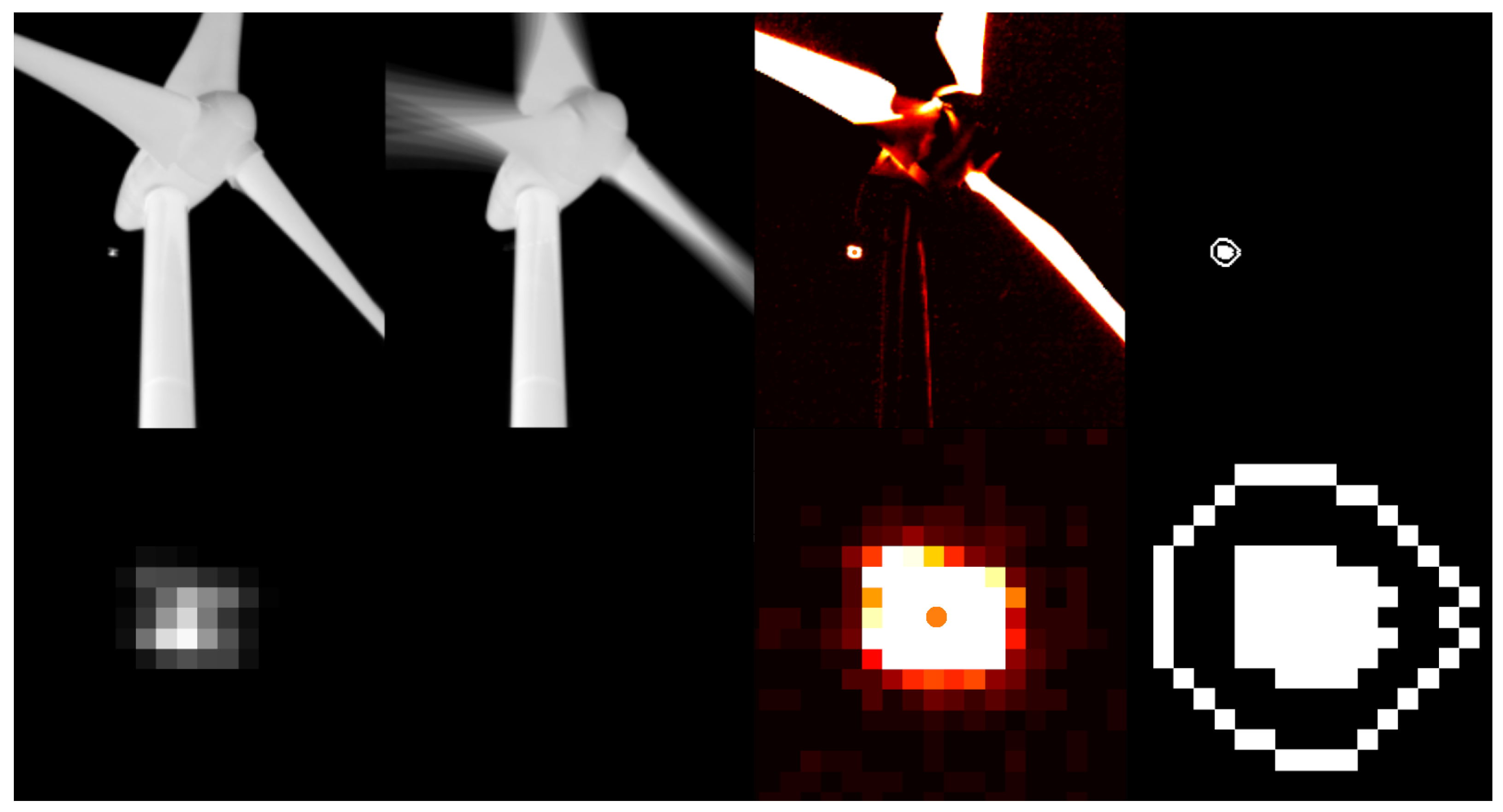
Image points and are detected by the image-processing methods background subtraction, thresholding, morphological operations (erosion and dilation) and blob analysis with the Python module scikit-image 0.19.1 [47]. The background subtraction extracts regions with movement (column 3 in Figure 8) by building up a background image consisting of the median pixels of past images, followed by thresholding. The result are regions which become modified by the morphological operations and labeled to find distinct candidates for further 2D processing (more details can be found in Appendix E). Each candidate consists of an inner part and a border (column 4) and can be analyzed by blob analysis, deciding whether to keep or dismiss them by thresholding for their median intensity, intensity differences (between inner region and border), sizes, eccentricity and other parameters. The intensity difference between the inner region and the border helps reduce false positives, such as those caused by partially detected rotor blades. The final 2D point coordinates are defined by their intensity-weighted centers of gravity. The exact thresholding parameters are found experimentally and depend on the used thermal cameras (image format, resolution, bit depth and the NETD (Noise Equivalent Temperature Difference)) and the weather (clouds, temperature and humidity). The attached code [43] provides a 3D-calibration example, including the complete 2D detection with all adjustable 2D measures and parameters.

Figure 8.
Example 2D detection of the drone in a distance of 48 m. Image 1 of each row is the current image, image 2 is the background image (movement of the turbine can be seen), image 3 is the background subtracted image with its intensity-weighted center of gravity (orange) and image 4 is the thresholded image with its inner region and the border.
The background subtracted image in column 3 in Figure 8 shows a high sensibility, which is necessary to detect drones in larger distances (see Figure 5). This holds also for the detection of bats as their thermal signature is even lower. Images of bats can be found in Appendix D.
3.6. Corresponding Image Points of Both Cameras
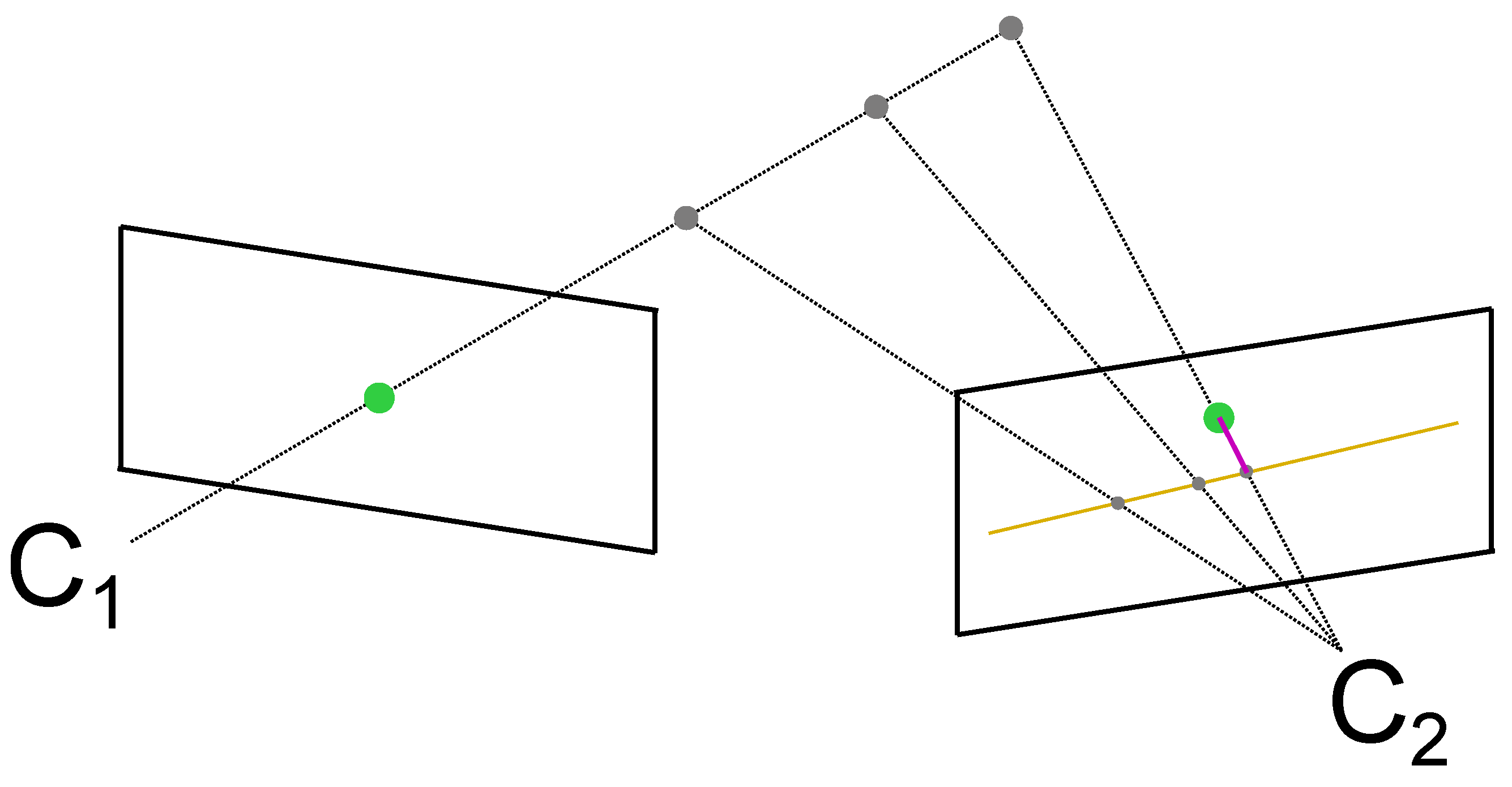
After performing the 2D image point detection separately for both cameras, the next step is to find the correspondences between points in both cameras. Based on the preliminary calibration, epipolar geometry is used to find the correspondences. This is based on the idea that for a known 3D calibration, points in one camera map to lines in the second camera as [48] suggested. This can be seen in Figure 9. A point in the image plane of the first camera maps to a line in the image plane of the second camera because of the already known epipolar geometry based on the 3D calibration. Therefore, this line has to be searched for the corresponding object. Because the 3D calibration as well as the object detection algorithms are not exact, a threshold defines the allowed distance to this line (illustrated in pink). Figure 10 shows one example of how this principle is used on our image data to find the corresponding drone points.
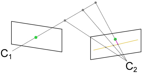
Figure 9.
A point (green) from the image plane of the first camera maps to a line (orange) in the image plane of the second camera . The distance of a potential detection from the epipolar line (pink) is used as a measure to threshold for correspondence.
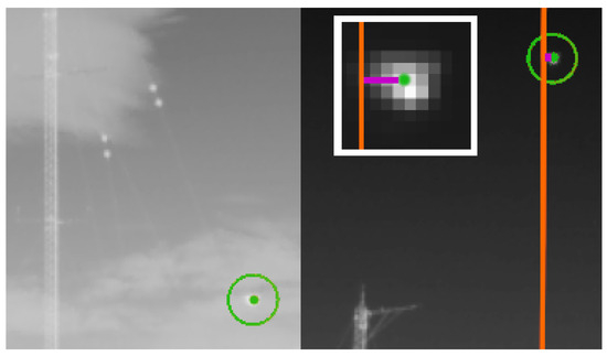
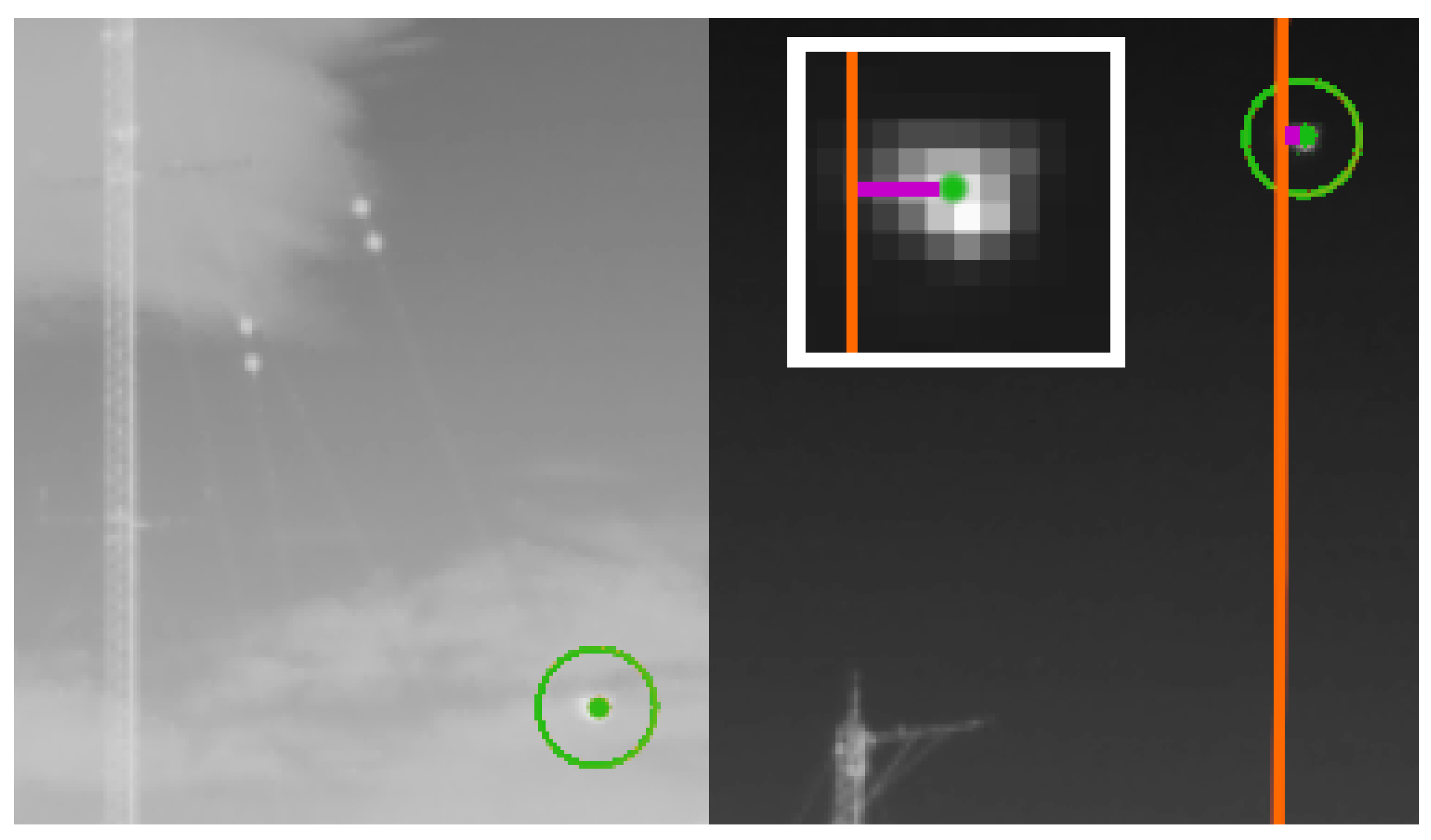
Figure 10.
Example of the use of epipolar geometry to find corresponding points. The same colors as in Figure 9 are used. The white border is a zoomed version of the second camera image showing the threshold (pink) on a pixel level.
All points without a corresponding partner are dismissed; they are either noise related or objects that are not present in both cameras because they are too close to one camera. After this step, and share the same number of elements.
4. Results
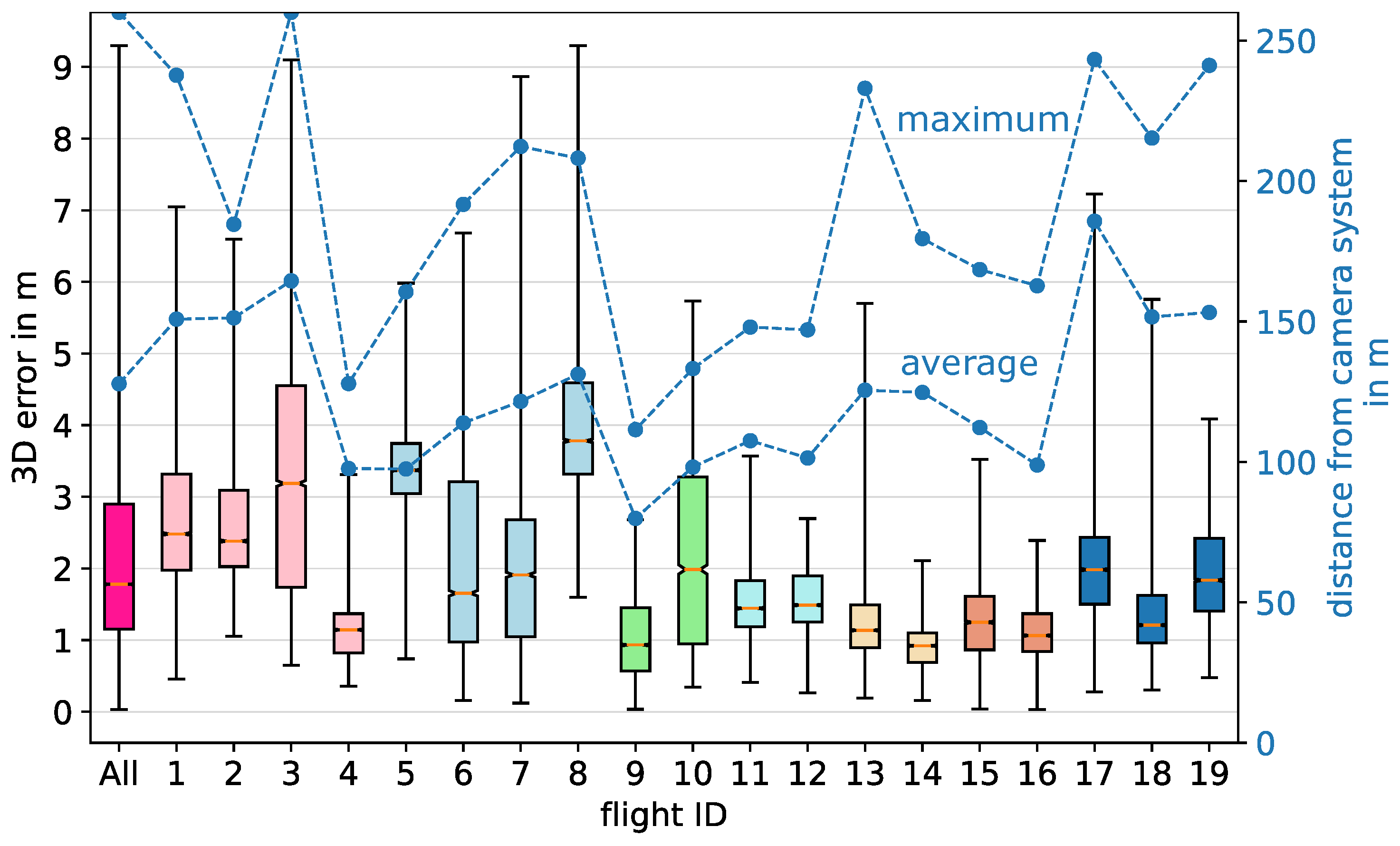
Following the methodology, we carried out 19 independent flights at two different locations, with 6 different camera setups. For each setup, we performed a minimum of two UAV flights in order to use one flight at a time for reconstruction/evaluation and the others for 3D calibration. All flights were performed manually and independently of one another. Each time we sought to cover significant parts of the measurement volume. The flights lasted between 3.9 and 12.6 min with an average of 7.7 min. The mean UAV distance from the camera system over all flights was 122 m, with individual values ranging from 33 m to 260 m. The 19 UAV flights lead to 19 3D error boxplots by cross-validation, reflecting the 3D-calibration quality (Figure 11).

Figure 11.
Cross-validated 3D errors between reconstructed points and UAV GPS points. The same color indicates the same camera setup. For example, Flight 2 is validated against a 3D calibration of flights 1, 3 and 4. The first boxplot in pink sums up the errors of all others.
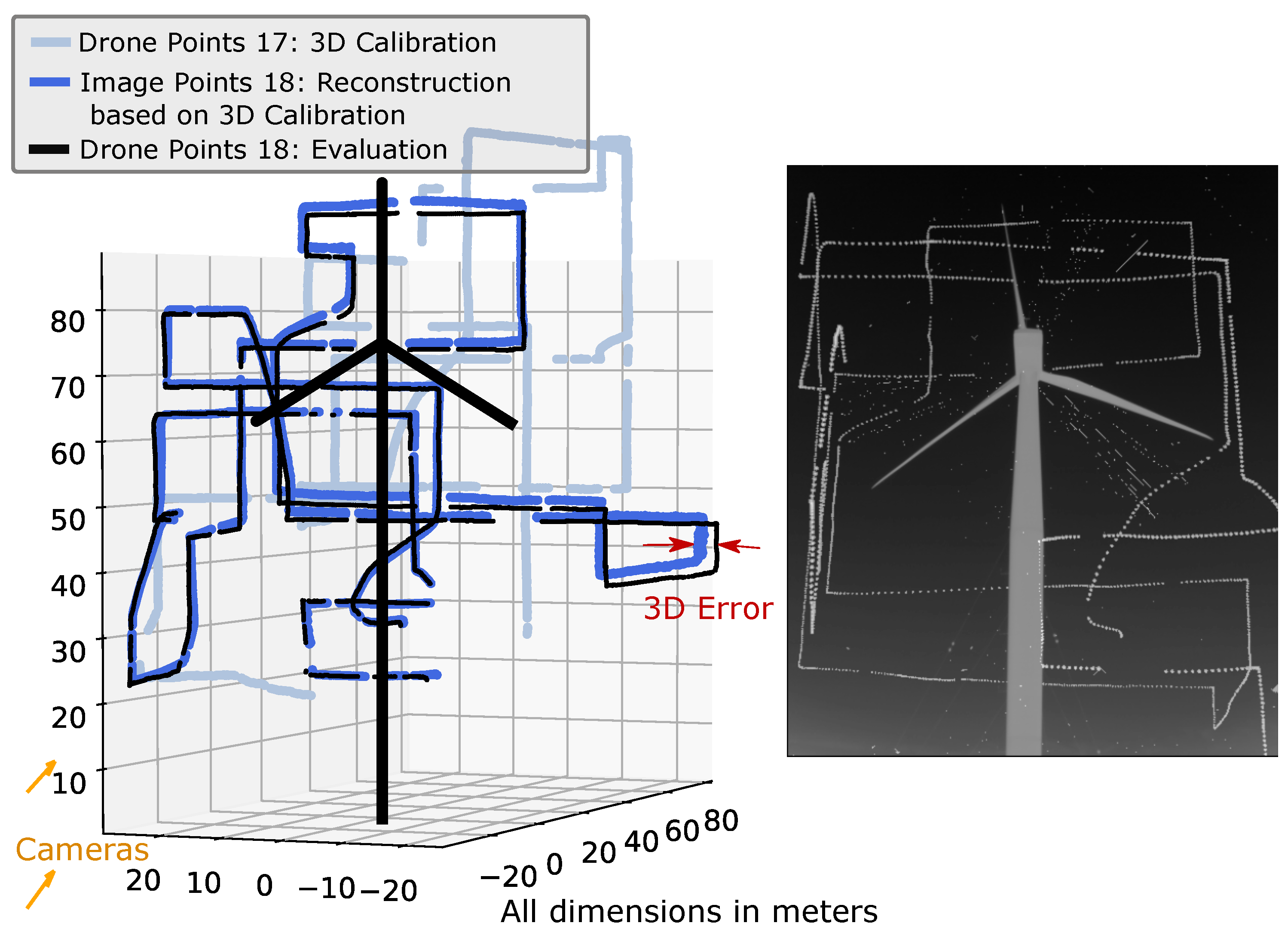
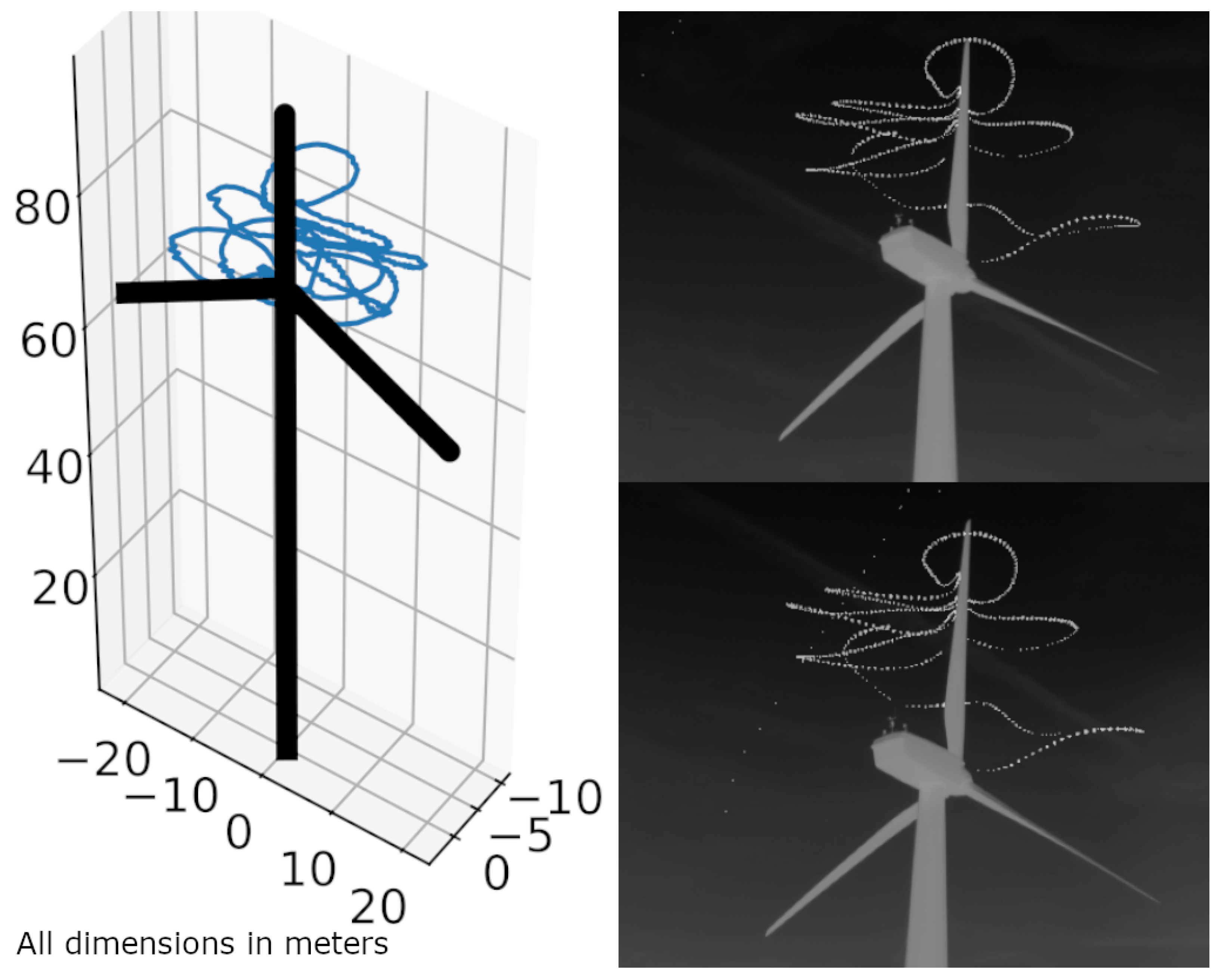
Before analyzing the 3D error results across all flights, we show the errors of flight 18 as an example. Flights 17 and 18 in Figure 12 are performed with the same camera setup. The image points of flight 18 (dark blue) are reconstructed and compared to the UAV GPS points of flight 18 (black) by the 3D error. In this case, flight 18 corresponds to the blue UAV dataset in Figure 2. The 3D calibration is performed by using the points of flight 17 (light blue). These correspond to the red UAV dataset in Figure 2. This is performed in the same way for all other flights. Their resulting 3D errors can be seen in Figure 11. All 3D plots can be reproduced and viewed as in Figure 12 for all 3D error bars in Figure 11 with the attached software and data [43].

Figure 12.
(Left): Example reconstruction of flight m = 18: UAV points of flight n = 17 are used for calibration (light blue), the 3D errors of the 3D reconstructed image points (dark blue) and UAV points (black) are used for an independent evaluation. (Right): Cumulative drone flight track 18 seen from camera 1.
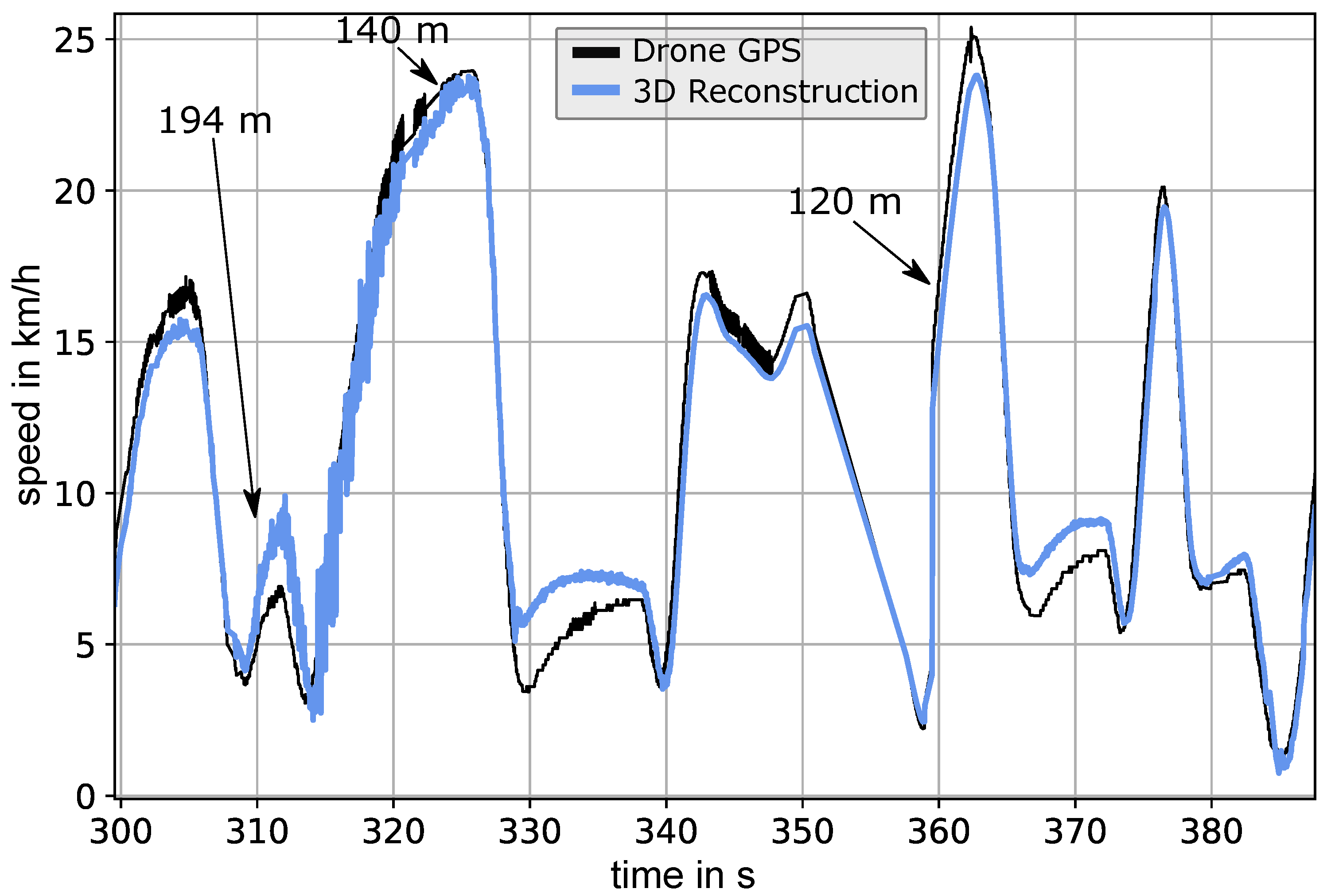
The median 3D errors per flight are between 0.92 m and 3.78 m, with a median of 1.78 m over all calibration flights. In order to see if this accuracy is sufficient for calculating a speed curve, we plotted a comparison between the UAV GPS and the 3D reconstruction in Figure 13.
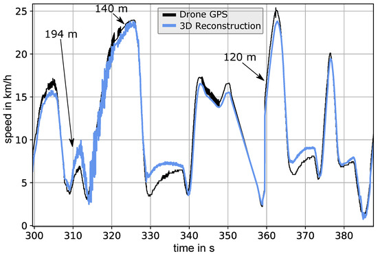
Figure 13.
Calculated speed of the UAV according to GPS (black) and the 3D-reconstructed UAV points (blue) of flight 1. It was calculated by taking the difference quotient with a of two seconds (smoothing). The arrows mark the distance of the UAV to the camera system.
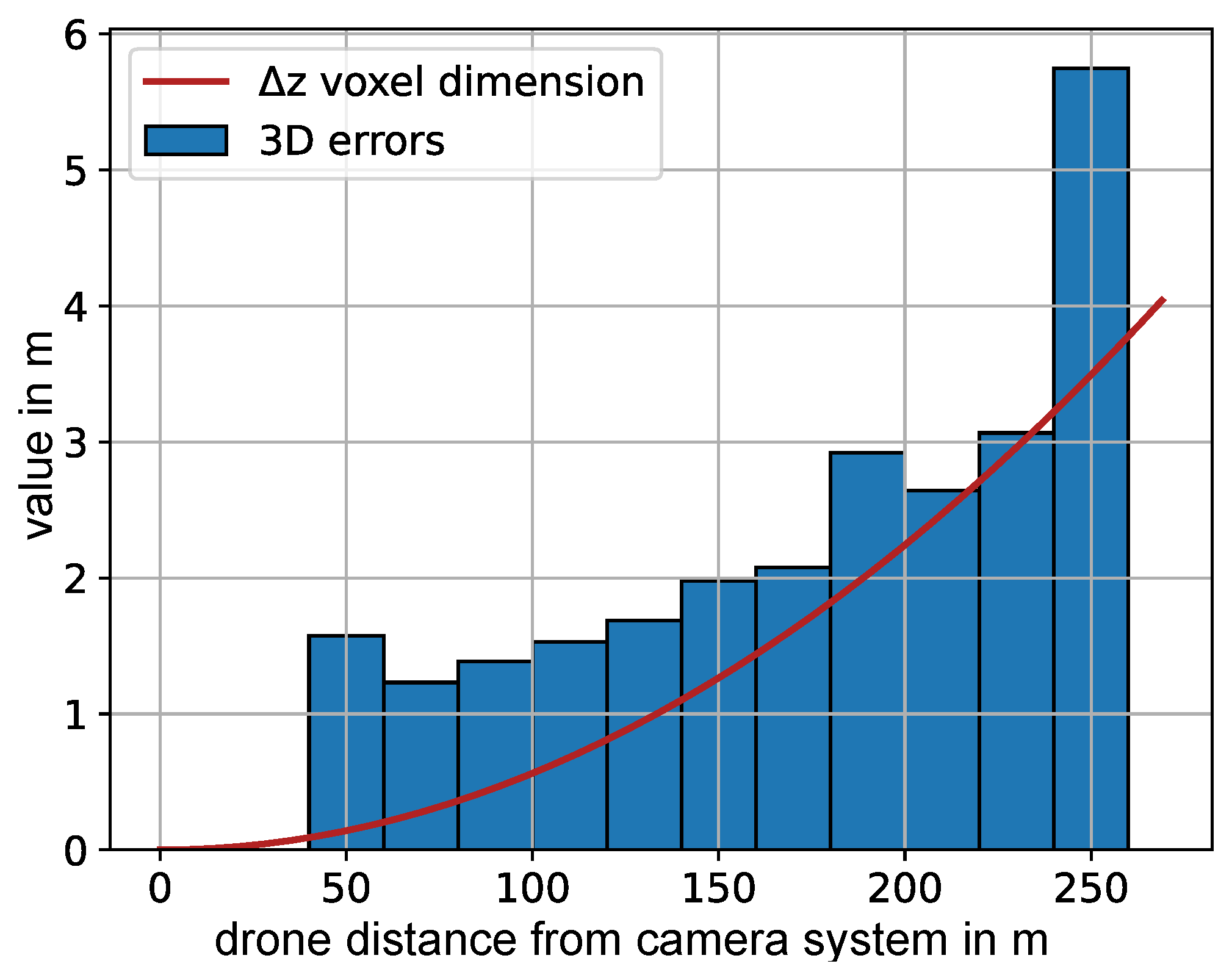
We also investigated the dependency of the 3D error on the distance from the camera system. Therefore, we sorted the 3D errors of all flights according to the corresponding UAV distance to the camera system and grouped them in intervals of 20 m (Figure 14). The overlaid red curve shows the theoretical projected voxel dimension in the depth direction.

Figure 14.
Theoretical curve of projected voxel in the depth dimension for the given cameras according to Appendix A (red) and dependency of the 3D error on the distance from the camera system calculated over all calibration flights (blue).
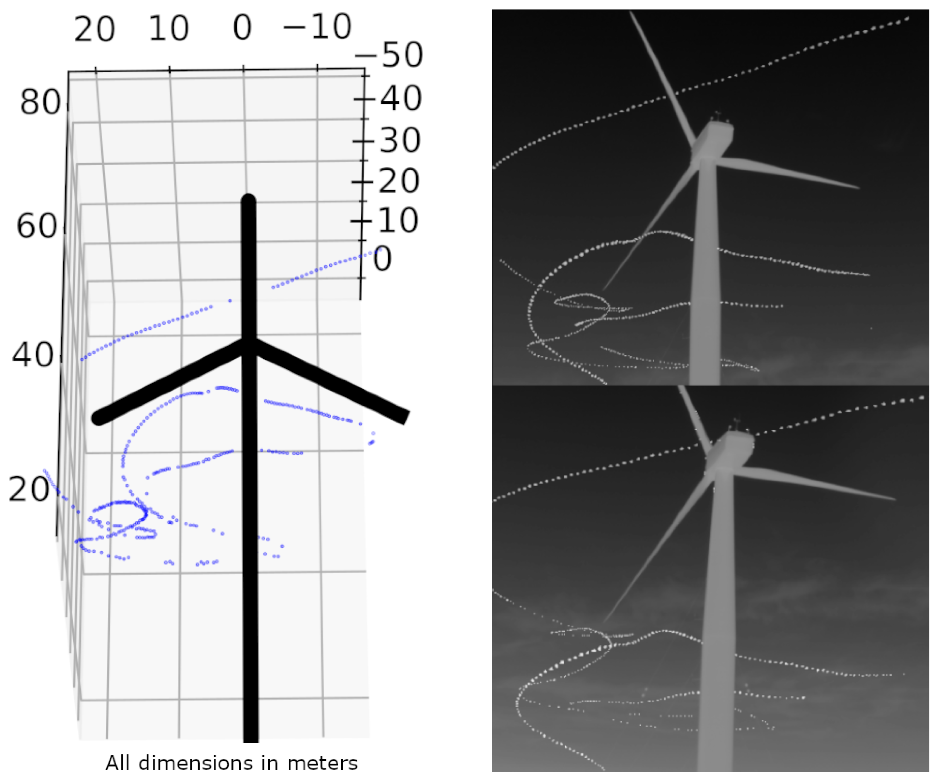
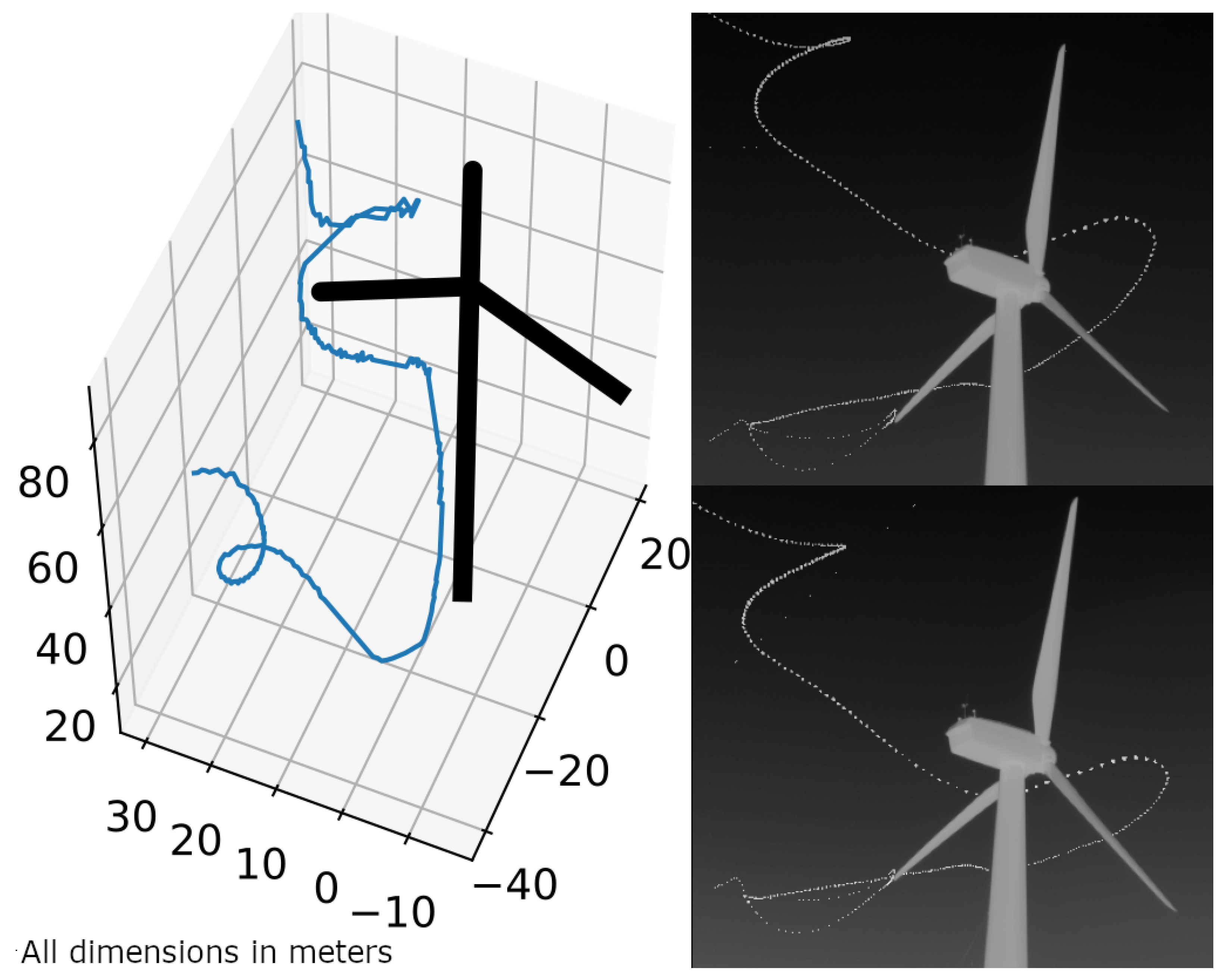
Since the main use case of this method is to derive flight tracks of nocturnal flying animals, we finally present examples with flight tracks. Figure 15 contains an individual on the 9 August 2024 at 1:10 a.m. at a wind turbine site in Kuchalb, Germany, with a flight track that appears to avoid the rotor swept area.

Figure 15.
The 3D-reconstructed flight track of an individual avoiding the rotor swept area (left). Same cumulative flight track seen from both cameras (right). Location: Kuchalb, Germany. Speed and height graphs derived from this flight track are shown in Figure 16.
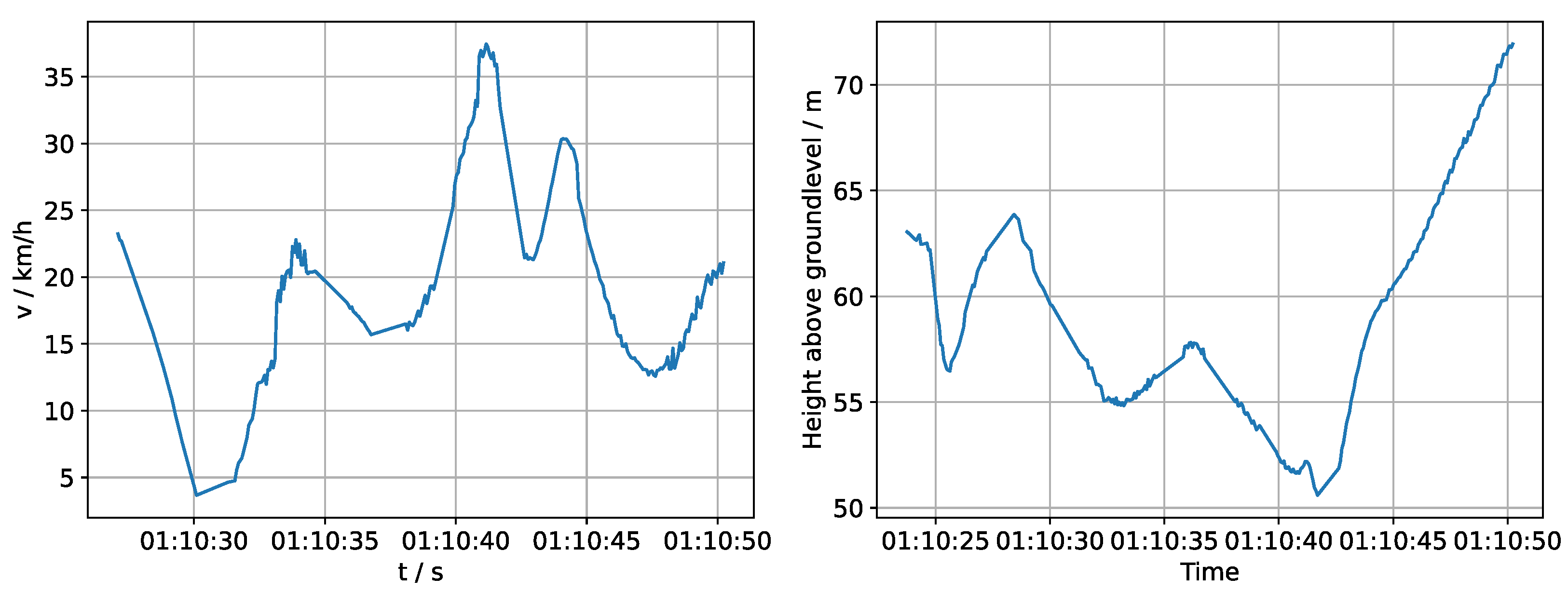
In Figure 16, two possible derivatives (speed and height above ground) can be seen which can be calculated from the flight track. More possibilities include, e.g., geographical heading, distance to the turbine or a 2D projection.
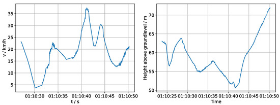
Figure 16.
Speed (left) and height above ground curve (right) of the flight track in Figure 15.
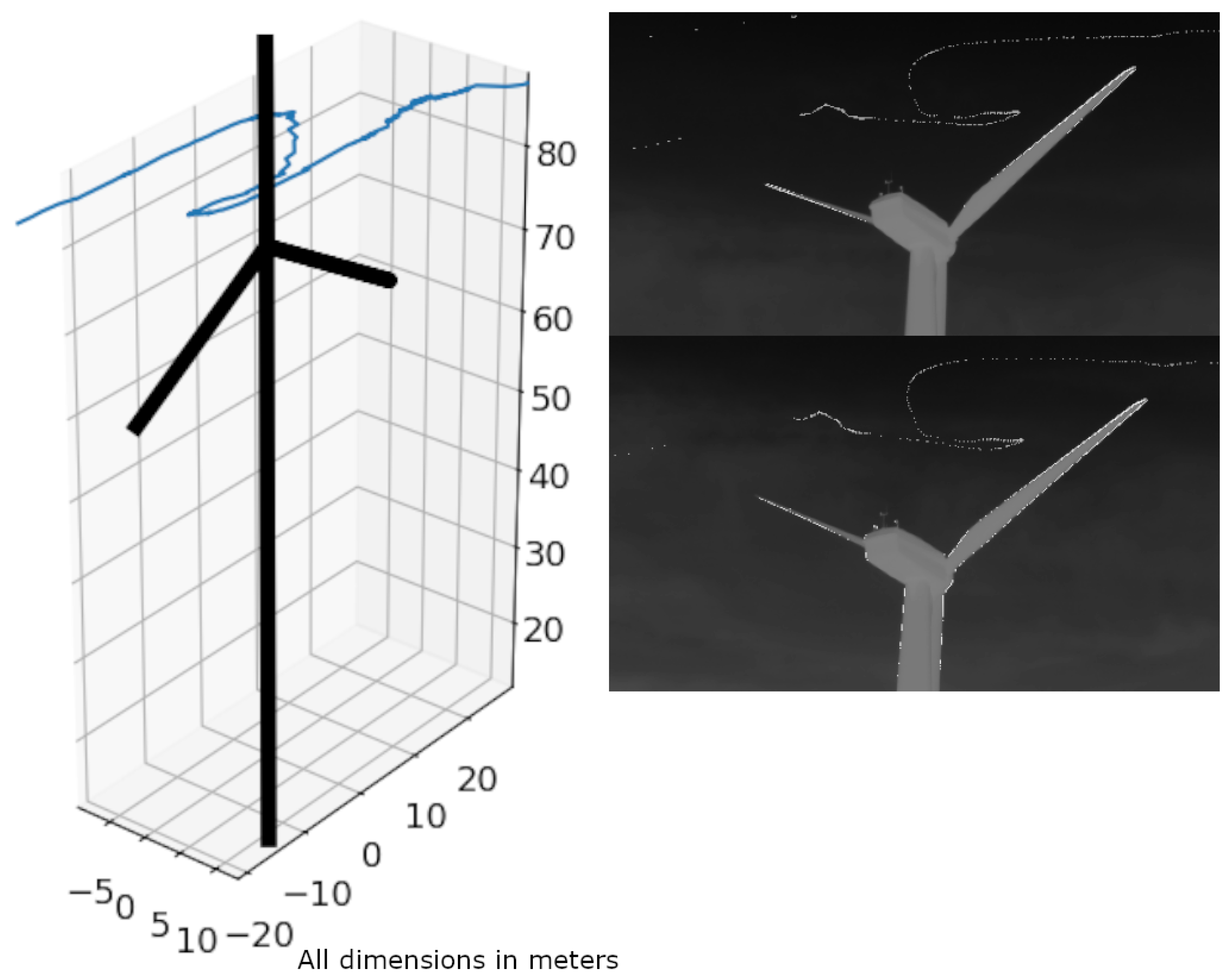
Figure 17 shows an individual that predominantly stays in the the rotor swept area.

Figure 17.
The 3D-reconstructed flight track of an individual predominantly remaining within the rotor-swept area (left). Same cumulative flight track seen from both cameras (right). Location: Kuchalb, Germany.
We already gathered around 26 h of 3D flight tracks, mainly in the summer season 2024. Their interpretation is the subject of a future work, but there are a few more examples of already-measured flight tracks in Appendix C, including flight tracks where we could identify the bat species by acoustic monitoring.
5. Discussion
In this section, we interpret the above results in the context of automatic bat flight detection. Figure 11 shows that the median errors of the 3D calibration flights vary between 0.92 and 3.78 m. The error variance has two main causes. The first is the human factor of performing the UAV flights manually.
Although the flights are performed to cover the measurement volume as evenly as possible, variation does still occur between them. The second cause is the distance to the camera system. For flights where the maximum UAV distance is higher (e.g., flight 3), the errors are naturally higher. Flights 9–16 are performed at a location where the measurement volume was smaller, and therefore, the median errors are also smaller. This can be seen by the average distance from the camera system. Although the error and its variation can be improved by performing automated UAV flights, we wanted to provide a 3D-calibration method which can be performed simply with a consumer UAV. Despite the variance in the errors, these errors are still by an order of magnitude small enough to allow for accurate results for bat detection (median errors of about 1 to 4 m in distances between 30 and 260 m). In addition, the accuracy of our method allows us to directly derive a speed curve, as shown in the results of Figure 13). There, we see that the speed derived by the reconstructed points follows the GPS curve, allowing for not only bat 3D flight tracks, but their corresponding speed profiles. We finally analyzed 3D errors dependent on their distance from the camera system for all calibration flights (Figure 14). The median 3D error (blue) grows similarly to the depth dimension of a projected voxel (red). This helps to estimate the 3D errors for a camera system based on its voxel depth curve.
The major difference to the existing methods referred to in the Introduction is the use of a dynamic 3D-calibration object across the whole measurement volume. The UAV flight track can be flexibly chosen in terms of homogeneity, density and size of the measurement volume. This allows for a large distance between the cameras, which is essential to achieve high 3D reconstruction accuracy in large outdoor volumes with low-resolution (thermal) cameras. Further, this allows us to directly measure the 3D-calibration quality in metric units. Without this, only an RMSE between the observed and the reprojected points in 2D can be calculated. This is a measure of the projective transformation obtained by the point correspondences and does not give an answer to the question if the perspective and the scale ambiguity are properly solved. Therefore, the final position of the 3D points is still uncertain and highly dependent on the accuracy of the intrinsic parameters. In contrast, we directly choose the extrinsic camera parameters to fit the 3D UAV GPS flight track. This provides the advantages of not needing further coordinate system transformations based on additional measurements, plus, we can directly calculate the speed and compass direction of the measured animals.
One limitation of the method is the dependency on the UAV GPS accuracy and flight regulations. So, it can be used where the GPS signal works properly, where it is legal to fly the UAV and where the GPS error is orders of magnitude smaller than the measured volume. To make the method applicable for smaller volumes, high-precision RTK UAVs could possibly be used. Another limitation is the manual flight behavior of the UAV pilot. It needs some practice and spatial sense to carry out proper calibration flights. The concatenation of more flights makes it possible to diminish that factor. Another solution could be to use an automated UAV and calculate a flight track for an optimal point cloud distribution. Using stereo cameras for 3D flight-track detection causes a non-uniform spatial voxel resolution depending on the distance from the camera system (Figure A2). So, even if the bat can still be detected, the spatial resolution may not be enough at some distances to represent the complex flight behaviour of bats. Another limitation from the biological perspective is the difficulty of detecting the species of the flying animals due to the low-resolution cameras. A solution to that problem is to combine the method with acoustic monitoring to obtain species information, which is the subject of ongoing work. We also want to carry out further research on how the detection probability of bats depends on the distance from the camera system and how we can measure and lower this dependency through image-processing methods.
6. Conclusions
We introduced a UAV-based method to detect the 3D flight trajectories of flying bats with thermal cameras in large outdoor environments. This method was implemented at two wind farms in Germany with a median calibration error of 1.8 m for monitoring volumes of the order of 30–260 m. By directly providing geographical coordinates and reliable 3D errors in metric units, we overcome several problems of existing approaches. As a result, we automatically detected thousands of 3D flight tracks of bats at these two locations. A technical limitation of this method is the individual factor in the design of the manual UAV flight track influencing the 3D calibration quality. This could be improved with an automatic UAV flight pattern if necessary. In addition the current accuracy of our method is limited by that of the GPS signal of the consumer UAV used, which can be further improved by using RTK UAVs. Finally, the low-resolution cameras limit the possibility to determine the species directly from the images. This can be overcome by combination with acoustic monitoring, which is the subject of ongoing work.
Author Contributions
Conceptualization, K.H.; data curation, C.H. and K.H.; formal analysis, C.H.; funding acquisition, K.H.; investigation, C.H.; methodology, C.H.; project administration, A.S.; resources, C.H. and K.H.; software, C.H.; supervision, K.H.; validation, C.H. and K.H.; visualization, C.H.; writing—original draft, C.H.; writing—review and editing, C.H., A.S. and K.H. All authors have read and agreed to the published version of the manuscript.
Funding
This research was funded by the German Federal Agency for Nature Conservation grant number 3523 15 1900 (NatForWINSENT II – 2).
Data Availability Statement
The Python code and the data which are necessary to reproduce the graphs in the results section in this publication are openly available at: https://github.com/christofhapp/batflight3D_publication/tree/v1.0.1 (accessed on 2 October 2024).
Acknowledgments
We would like to thank Catherine Laflamme for her help in improving the writing style of this manuscript with her native English skills.
Conflicts of Interest
The authors declare no conflicts of interest.
Abbreviations
The following abbreviations are used in this manuscript:
| DLT | Direct Linear Transform |
| GLONSASS | Global Navigation Satellite System |
| GPS | Global Positioning System |
| HFOV | Horizontal Field of View |
| IMG | Image(s) |
| NETD | Noise-Equivalent Temperature Difference |
| RMSE | Root Mean Squared Error |
| RTK | Real-time Kinematic Positioning |
| UAV | Unmanned Aerial Vehicle |
| UTM | Universal Transverse Mercator (earth coordinate system (projected, metric)) |
| WGS 84 | World Geodetic System 1984 (earth coordinate system (ellipsoid)) |
Appendix A. Camera Inter-Axial Distance and Its Effects on the 3D Resolution
Given the above hardware parameters, we chose an inter-axial distance between the cameras of about 15 m (either vertical or horizontal). This was decided based on the following considerations.
From the geometric principle of stereo triangulation, it can be found that the resolution and the inter-axial distance of the cameras, among others, determine the resolution of a voxel (volume pixel) in space. Referring to Figure A3, the voxel size of the parallel plane to the image sensor and is different from the common orthogonal direction (Equations (A4) and (A3)).
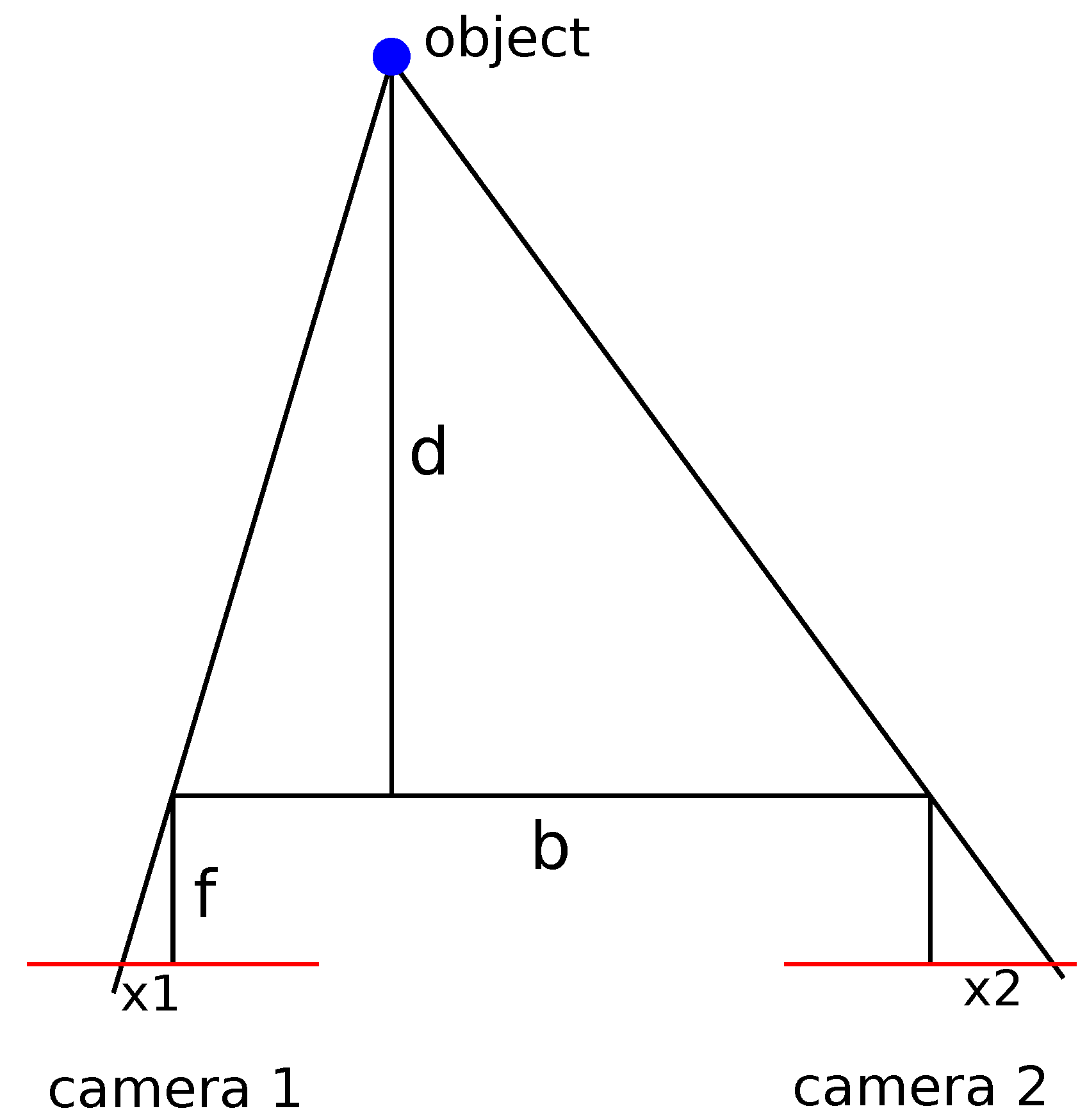
If, according to Figure A1, d is the distance from the camera system, f is the focal length of the cameras, b is the inter-axial distance between the cameras, is the disparity and a is the sensor pixel length, then the following holds because of the similarity theorem:
is the resolution in the depth direction and is defined by:
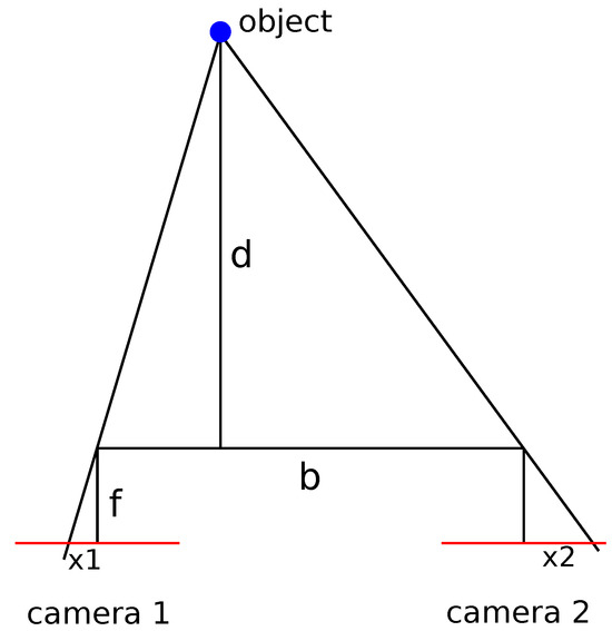
Figure A1.
Scheme of a parallel 3D camera system and the line of sight to an object; d is the distance from the camera system, f is the focal length of the cameras, b is the inter-axial distance between the cameras and is the disparity.
Figure A1.
Scheme of a parallel 3D camera system and the line of sight to an object; d is the distance from the camera system, f is the focal length of the cameras, b is the inter-axial distance between the cameras and is the disparity.
Equation (A3) shows that the resolution of the z-direction is linearly connected to the distance between the cameras b (if we assume that and d is negligible). A higher distance between the cameras on the other hand has the drawback of a smaller overlapping volume. The system described results in the voxel dimensions shown in Figure A3. Figure A2 shows the resulting voxel sizes for different distances from the camera system.
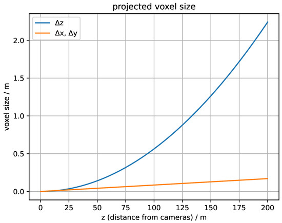
Figure A2.
Projected voxel size (b = 15 m, a = 17 μm, f = 20 mm).
Figure A2.
Projected voxel size (b = 15 m, a = 17 μm, f = 20 mm).
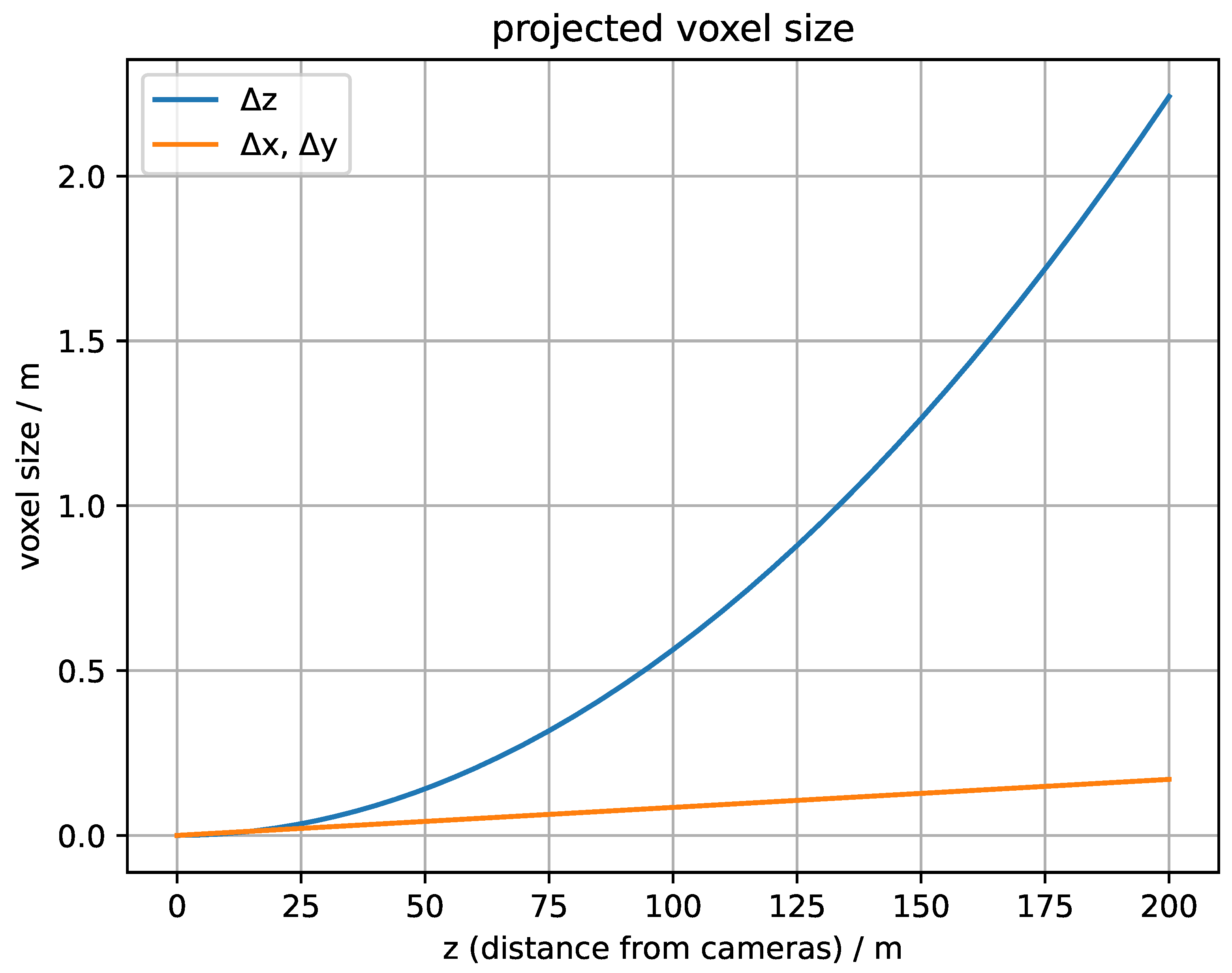
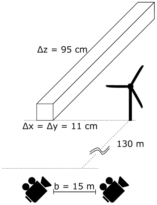
Figure A3.
Voxel dimensions in 130 m distance from our camera system.
Figure A3.
Voxel dimensions in 130 m distance from our camera system.
Appendix B. Single Camera Calibration
The single camera calibration is a prerequisite to the method and is used for determining the intrinsic parameters of the cameras (focal length, lens distortion and optical center). They can be either calculated from the specification sheet of the manufacturer or be determined by using the checkerboard method from [22] for single cameras. If exposed to direct sunlight, printed checkerboards also work for thermal cameras because of the different absorption coefficients of the white and black squares. This can be seen in Figure A4 for our cameras.

Figure A4.
Printed checkerboard pattern exposed to sunlight filmed by a thermal camera.
Figure A4.
Printed checkerboard pattern exposed to sunlight filmed by a thermal camera.
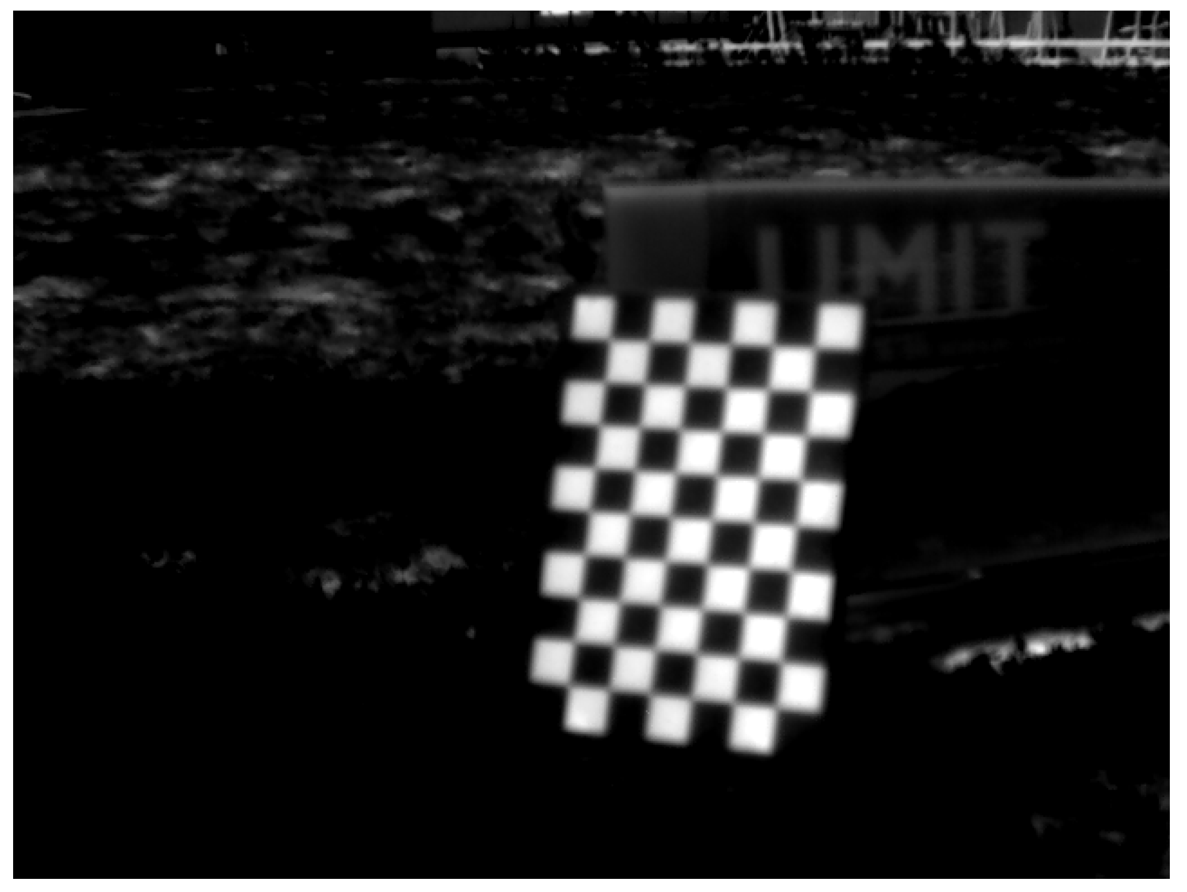
However, focusing on the checkerboard, which is much closer than our objects of interest, results in a focal shift due to optical aberration. That is why we finally calculated the intrinsic matrices and the distortion matrices from the specification sheet. The values for the intrinsic matrix are given in pixels, but the data sheet usually provides the sensor pixel size and focal length in metric units. To obtain the focal length f in pixels, the focal length has to be devided by the sensor pixel length a:
For our cameras, mm, μm, resulting in . Further, we assumed our principal point to be in the image center with no distortions.
Appendix C. More Examples of 3D Flight Tracks
In this section, we provide more examples of 3D flight tracks.
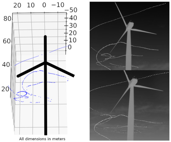
Figure A5.
The 3D-reconstructed flight track (left) of one individual on the 31 August 2024 at 04:01 a.m. in Kuchalb, Germany. The camera views with the accumulated flight can be seen on the (right).
Figure A5.
The 3D-reconstructed flight track (left) of one individual on the 31 August 2024 at 04:01 a.m. in Kuchalb, Germany. The camera views with the accumulated flight can be seen on the (right).
Another two flight tracks were recorded on the 26 June 2022 at 10:56 p.m. at a wind turbine site in Bavaria, Germany. They are shown in Figure A6. Animal 1 could be identified as a pipistrelle bat according to microphone recordings at the wind turbine tower. This example including the images and all the code for reconstruction is available at [43].
The following flight tracks of Figure A7 and Figure A8 are from the season 2024 and were chosen because we already received the acoustic data from this day.
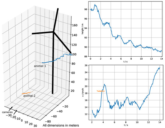
Figure A6.
The 3D-reconstructed flight tracks of two flying animals and their corresponding height and speed graphs. The black turbine model matches the size and geographical position of the real turbine. Location: Offenhausen, Germany.
Figure A6.
The 3D-reconstructed flight tracks of two flying animals and their corresponding height and speed graphs. The black turbine model matches the size and geographical position of the real turbine. Location: Offenhausen, Germany.
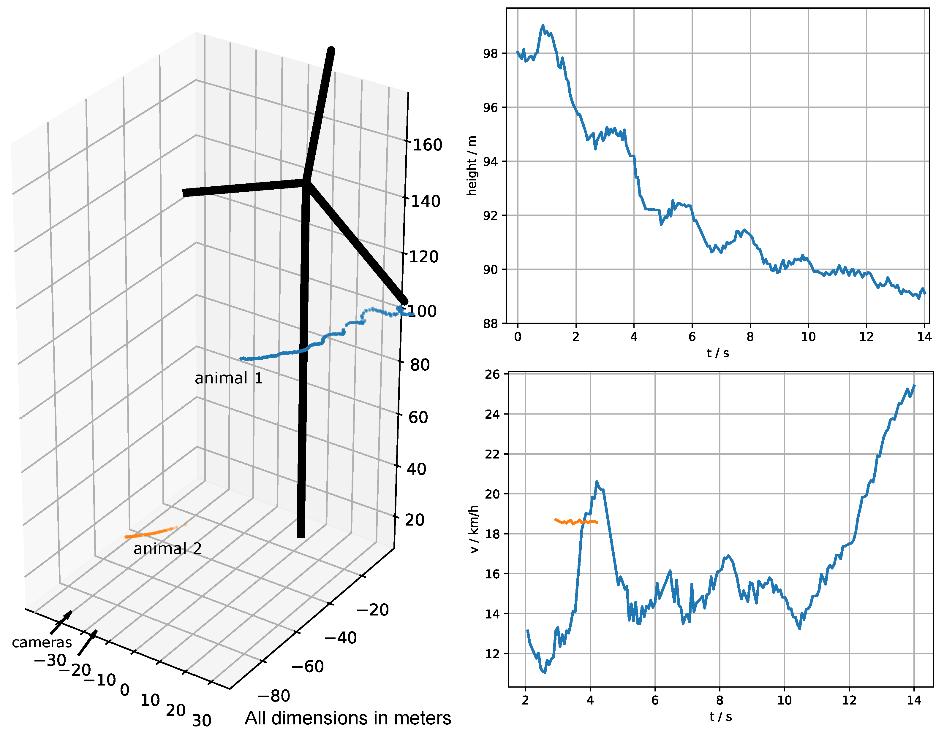
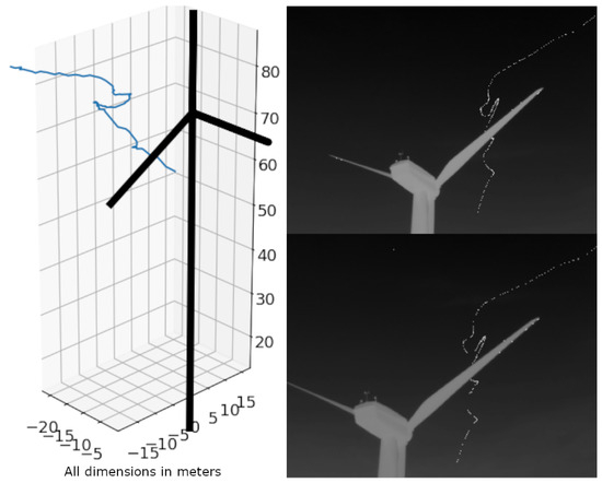
Figure A7.
The individual of this flight track could be identified as a pipistrelle bat through acoustic monitoring in the nacelle. Location: Kuchalb, Germany.
Figure A7.
The individual of this flight track could be identified as a pipistrelle bat through acoustic monitoring in the nacelle. Location: Kuchalb, Germany.


Figure A8.
The individual of this flight track could be identified as a noctule bat through acoustic monitoring in the nacelle. Location: Kuchalb, Germany.
Figure A8.
The individual of this flight track could be identified as a noctule bat through acoustic monitoring in the nacelle. Location: Kuchalb, Germany.
Appendix D. Example Images of Bats
As our measure volume has an average distance of about 130 m, we expect most captured bats to fill just one to a few pixels, as can be seen in Figure A9.

Figure A9.
Images of bats in different distances.
Figure A9.
Images of bats in different distances.
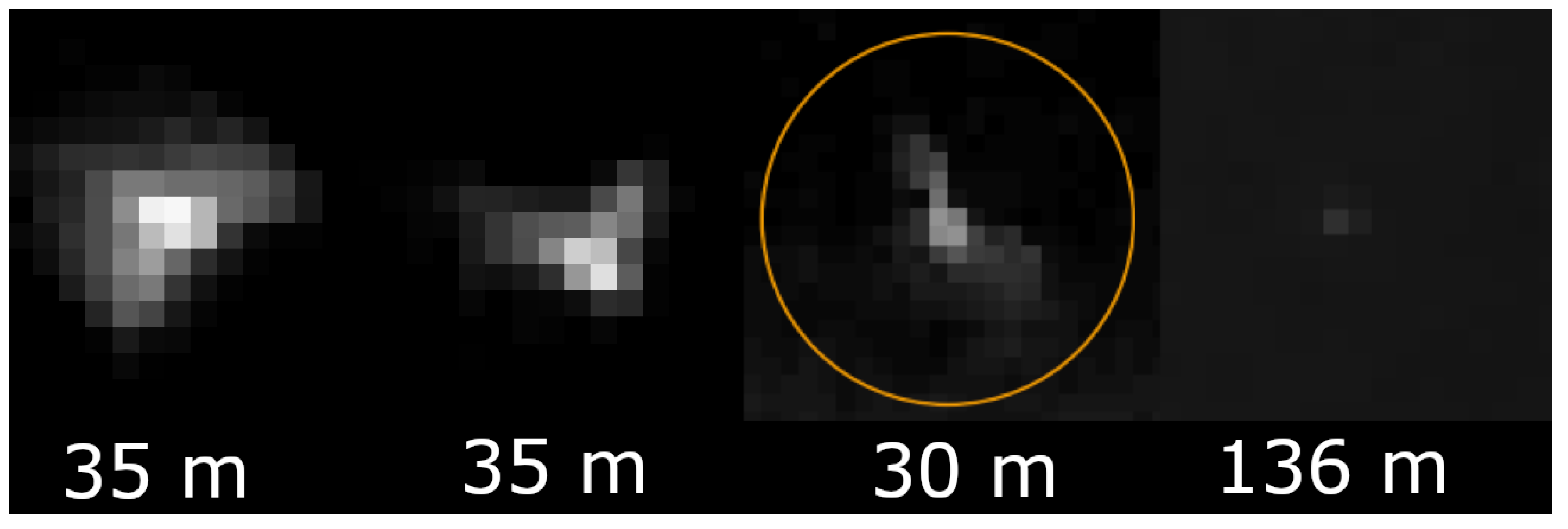
Identifying the species just from these images is not possible, but can be achieved by correlating the data with acoustic monitoring.
Appendix E. Morphological Operations as Part of the 2D Detection Process
Figure A10 shows how the thresholded regions are transformed and labeled for further analysis, so that it is possible to obtain distinct candidates with an inner region and a border around it. These categories help to perform further analysis on each candidate and also to analyze the inner parts and compare them to their direct surrounding (border).
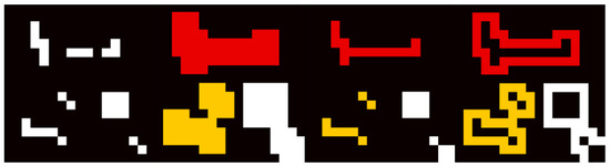
Figure A10.
1: Thresholded background subtraction; 2: candidates after several times of dilation and labeling; 3: inner parts after several times of erosion; 4: border by subtraction of dilation and erosion.
Figure A10.
1: Thresholded background subtraction; 2: candidates after several times of dilation and labeling; 3: inner parts after several times of erosion; 4: border by subtraction of dilation and erosion.
References
- European Commission. European Wind Power Action Plan. 2023. Available online: https://eur-lex.europa.eu/legal-content/EN/ALL/?uri=CELEX:52023DC0669 (accessed on 2 October 2024).
- Arnett, E.B.; Baerwald, E.F. Impacts of wind energy development on bats: Implications for conservation. In Bat Evolution, Ecology, and Conservation; Springer: Berlin/Heidelberg, Germany, 2013; pp. 435–456. [Google Scholar] [CrossRef]
- Kunz, T.H.; Arnett, E.B.; Erickson, W.P.; Hoar, A.R.; Johnson, G.D.; Larkin, R.P.; Strickland, M.D.; Thresher, R.W.; Tuttle, M.D. Ecological impacts of wind energy development on bats: Questions, research needs, and hypotheses. Front. Ecol. Environ. 2007, 5, 315–324. [Google Scholar] [CrossRef]
- Göttert, T.; Starik, N. Human–wildlife conflicts across landscapes—General applicability vs. case specificity. Diversity 2022, 14, 380. [Google Scholar] [CrossRef]
- Baerwald, E.F.; D’Amours, G.H.; Klug, B.J.; Barclay, R.M. Barotrauma is a significant cause of bat fatalities at wind turbines. Curr. Biol. 2008, 18, R695–R696. [Google Scholar] [CrossRef] [PubMed]
- Guest, E.E.; Stamps, B.F.; Durish, N.D.; Hale, A.M.; Hein, C.D.; Morton, B.P.; Weaver, S.P.; Fritts, S.R. An updated review of hypotheses regarding bat attraction to wind turbines. Animals 2022, 12, 343. [Google Scholar] [CrossRef] [PubMed]
- Cryan, P.M. Mating behavior as a possible cause of bat fatalities at wind turbines. J. Wildl. Manag. 2008, 72, 845–849. [Google Scholar] [CrossRef]
- Rydell, J.; Bach, L.; Dubourg-Savage, M.J.; Green, M.; Rodrigues, L.; Hedenström, A. Mortality of bats at wind turbines links to nocturnal insect migration? Eur. J. Wildl. Res. 2010, 56, 823–827. [Google Scholar] [CrossRef]
- Cryan, P.M.; Gorresen, P.M.; Hein, C.D.; Schirmacher, M.R.; Diehl, R.H.; Huso, M.M.; Hayman, D.T.; Fricker, P.D.; Bonaccorso, F.J.; Johnson, D.H.; et al. Behavior of bats at wind turbines. Proc. Natl. Acad. Sci. USA 2014, 111, 15126–15131. [Google Scholar] [CrossRef] [PubMed]
- Reusch, C.; Lozar, M.; Kramer-Schadt, S.; Voigt, C.C. Coastal onshore wind turbines lead to habitat loss for bats in Northern Germany. J. Environ. Manag. 2022, 310, 114715. [Google Scholar] [CrossRef]
- Voigt, C.C.; Russo, D.; Runkel, V.; Goerlitz, H.R. Limitations of acoustic monitoring at wind turbines to evaluate fatality risk of bats. Mammal Rev. 2021, 51, 559–570. [Google Scholar] [CrossRef]
- Voigt, C.C.; Scherer, C.; Runkel, V. Modeling the power of acoustic monitoring to predict bat fatalities at wind turbines. Conserv. Sci. Pract. 2022, 4, e12841. [Google Scholar] [CrossRef]
- Horn, J.W.; Arnett, E.B.; Kunz, T.H. Behavioral responses of bats to operating wind turbines. J. Wildl. Manag. 2008, 72, 123–132. [Google Scholar] [CrossRef]
- Betke, M.; Hirsh, D.E.; Makris, N.C.; McCracken, G.F.; Procopio, M.; Hristov, N.I.; Tang, S.; Bagchi, A.; Reichard, J.D.; Horn, J.W.; et al. Thermal imaging reveals significantly smaller Brazilian free-tailed bat colonies than previously estimated. J. Mammal. 2008, 89, 18–24. [Google Scholar] [CrossRef]
- Bentley, I.; Kuczynska, V.; Eddington, V.M.; Armstrong, M.; Kloepper, L.N. BatCount: A software program to count moving animals. PLoS ONE 2023, 18, e0278012. [Google Scholar] [CrossRef] [PubMed]
- Bentley, I.; Gebran, M.; Vorderer, S.; Ralston, J.; Kloepper, L. Utilizing Neural Networks to Resolve Individual Bats and Improve Automated Counts. In Proceedings of the 2023 IEEE World AI IoT Congress (AIIoT), Virtual, 7–10 June 2023; IEEE: Piscataway Township, NJ, USA, 2023; pp. 0112–0119. [Google Scholar]
- Håkansson, J.; Quinn, B.L.; Shultz, A.L.; Swartz, S.M.; Corcoran, A.J. Application of a novel deep learning–based 3D videography workflow to bat flight. Ann. N. Y. Acad. Sci. 2024, 1536, 92–106. [Google Scholar] [CrossRef] [PubMed]
- Darras, K.; Yusti, E.; Knorr, A.; Huang, J.C.C.; Kartono, A.P. Sampling flying bats with thermal and near-infrared imaging and ultrasound recording: Hardware and workflow for bat point counts. F1000Research 2022, 10, 189. [Google Scholar] [CrossRef] [PubMed]
- Hochradel, K.; Häcker, T.; Hohler, T.; Becher, A.; Wildermann, S.; Sutor, A. Three-Dimensional Localization of Bats: Visual and Acoustical. IEEE Sensors J. 2019, 19, 5825–5833. [Google Scholar] [CrossRef]
- Robinson Willmott, J.; Forcey, G.; Vukovich, M. New Insights into the Influence of Turbines on the Behaviour of Migrant Birds: Implications for Predicting Impacts of Offshore Wind Developments on Wildlife. J. Phys. Conf. Ser. 2023, 2507, 012006. [Google Scholar] [CrossRef]
- Bottalico, F.; Niezrecki, C.; Jerath, K.; Luo, Y.; Sabato, A. Sensor-Based Calibration of Camera’s Extrinsic Parameters for Stereophotogrammetry. IEEE Sensors J. 2023, 23, 7776–7785. [Google Scholar] [CrossRef]
- Zhang, Z. A flexible new technique for camera calibration. IEEE Trans. Pattern Anal. Mach. Intell. 2000, 22, 1330–1334. [Google Scholar] [CrossRef]
- Li, H.; Wang, S.; Bai, Z.; Wang, H.; Li, S.; Wen, S. Research on 3D reconstruction of binocular vision based on thermal infrared. Sensors 2023, 23, 7372. [Google Scholar] [CrossRef] [PubMed]
- Liu, X.; Tian, J.; Kuang, H.; Ma, X. A stereo calibration method of multi-camera based on circular calibration board. Electronics 2022, 11, 627. [Google Scholar] [CrossRef]
- Zheng, H.; Duan, F.; Li, T.; Li, J.; Niu, G.; Cheng, Z.; Li, X. A Stable, Efficient, and High-Precision Non-Coplanar Calibration Method: Applied for Multi-Camera-Based Stereo Vision Measurements. Sensors 2023, 23, 8466. [Google Scholar] [CrossRef]
- Hochradel, K.; Hartmann, S.; Reers, H.; Luedtke, B.; Schauer-Weisshahn, H.; Thomsen, K.M.; Hoetker, H.; Brinkmann, R. Three-dimensional analysis of bat flight paths around small wind turbines suggests no major collision risk or behavioral changes. Mammal Res. 2022, 67, 83–98. [Google Scholar] [CrossRef]
- Matzner, S.; Warfel, T.; Hull, R. ThermalTracker-3D: A thermal stereo vision system for quantifying bird and bat activity at offshore wind energy sites. Ecol. Inform. 2020, 57, 101069. [Google Scholar] [CrossRef]
- Matzner, S.; Warfel, T.; Hull, R.; Williams, N. ThermalTracker-3D Offshore Validation Technical Report; Technical Report; Pacific Northwest National Laboratory (PNNL): Richland, DC, USA, 2022. [Google Scholar]
- Schneider, S.R.; Kramer, S.H.; Bernstein, S.B.; Terrill, S.B.; Ainley, D.G.; Matzner, S. Autonomous thermal tracking reveals spatiotemporal patterns of seabird activity relevant to interactions with floating offshore wind facilities. Front. Mar. Sci. 2024, 11, 1346758. [Google Scholar] [CrossRef]
- Son, J.Y.; Chernyshov, O.; Lee, C.H.; Park, M.C.; Yano, S. Depth resolution in three-dimensional images. JOSA A 2013, 30, 1030–1038. [Google Scholar] [CrossRef]
- Li, G.; Xu, Z.; Zhang, Y.; Xin, C.; Wang, J.; Yan, S. Calibration method for binocular vision system with large field of view based on small target image splicing. Meas. Sci. Technol. 2024, 35, 085006. [Google Scholar] [CrossRef]
- Gao, Z.; Gao, Y.; Su, Y.; Liu, Y.; Fang, Z.; Wang, Y.; Zhang, Q. Stereo camera calibration for large field of view digital image correlation using zoom lens. Measurement 2021, 185, 109999. [Google Scholar] [CrossRef]
- Corcoran, A.J.; Schirmacher, M.R.; Black, E.; Hedrick, T.L. ThruTracker: Open-source software for 2-D and 3-D animal video tracking. bioRxiv 2021, 2021-05. [Google Scholar] [CrossRef]
- Theriault, D.H.; Fuller, N.W.; Jackson, B.E.; Bluhm, E.; Evangelista, D.; Wu, Z.; Betke, M.; Hedrick, T.L. A protocol and calibration method for accurate multi-camera field videography. J. Exp. Biol. 2014, 217, 1843–1848. [Google Scholar] [CrossRef] [PubMed]
- Hartley, R.; Zisserman, A. Multiple View Geometry in Computer Vision; Cambridge University Press: Cambridge, UK, 2003. [Google Scholar]
- Lourakis, M.I.; Argyros, A.A. SBA: A software package for generic sparse bundle adjustment. ACM Trans. Math. Softw. (TOMS) 2009, 36, 1–30. [Google Scholar] [CrossRef]
- Happ, C.; Hochradel, K.; Sutor, A. Comparison of two 3D calibration methods for thermal imaging cameras to track bat flight paths near wind turbines. Tm-Tech. Mess. 2024, 91, 61–65. [Google Scholar] [CrossRef]
- Tripicchio, P.; D’Avella, S.; Camacho-Gonzalez, G.; Landolfi, L.; Baris, G.; Avizzano, C.A.; Filippeschi, A. Multi-Camera Extrinsic Calibration for Real-Time Tracking in Large Outdoor Environments. J. Sens. Actuator Netw. 2022, 11, 40. [Google Scholar] [CrossRef]
- Feng, W.; Zhang, S.; Liu, H.; Yu, Q.; Wu, S.; Zhang, D. Unmanned aerial vehicle-aided stereo camera calibration for outdoor applications. Opt. Eng. 2020, 59, 014110. [Google Scholar] [CrossRef]
- Fedorov, I.; Thörnberg, B.; Alqaysi, H.; Lawal, N.; O’Nils, M. A Two-Layer 3-D Reconstruction Method and Calibration for Multicamera-Based Volumetric Positioning and Characterization. IEEE Trans. Instrum. Meas. 2021, 70, 1–9. [Google Scholar] [CrossRef]
- Zhang, Y.; Yang, J.; Li, G.; Zhao, T.; Song, X.; Zhang, S.; Li, A.; Bian, H.; Li, J.; Zhang, M. Camera Calibration for Long-Distance Photogrammetry Using Unmanned Aerial Vehicles. J. Sens. 2022, 2022, 8573315. [Google Scholar] [CrossRef]
- van Andel, B.; Tobias Bieniek, T.I.B. utm Python Module. [Code]. 2012. Available online: https://github.com/Turbo87/utm (accessed on 2 October 2024).
- Happ, C. Batflight 3D. [Code, Dataset]. 2024. Available online: https://github.com/christofhapp/batflight3D_publication/tree/v1.0.1 (accessed on 2 October 2024).
- Haralick, R.M.; Lee, C.n.; Ottenburg, K.; Nölle, M. Analysis and solutions of the three point perspective pose estimation problem. In Proceedings of the CVPR, Maui, HI, USA, 3–6 June 1991; Volume 91, pp. 592–598. [Google Scholar]
- Quan, L.; Lan, Z. Linear n-point camera pose determination. IEEE Trans. Pattern Anal. Mach. Intell. 1999, 21, 774–780. [Google Scholar] [CrossRef]
- Terzakis, G.; Lourakis, M. A consistently fast and globally optimal solution to the perspective-n-point problem. In Proceedings of the European Conference on Computer Vision, Glasgow, UK, 23–28 August 2020; Springer: Berlin/Heidelberg, Germany, 2020; pp. 478–494. [Google Scholar] [CrossRef]
- Van der Walt, S.; Schönberger, J.L.; Nunez-Iglesias, J.; Boulogne, F.; Warner, J.D.; Yager, N.; Gouillart, E.; Yu, T. scikit-image: Image processing in Python. PeerJ 2014, 2, e453. [Google Scholar] [CrossRef] [PubMed]
- Zhang, Z. Determining the epipolar geometry and its uncertainty: A review. Int. J. Comput. Vis. 1998, 27, 161–195. [Google Scholar] [CrossRef]


Disclaimer/Publisher’s Note: The statements, opinions and data contained in all publications are solely those of the individual author(s) and contributor(s) and not of MDPI and/or the editor(s). MDPI and/or the editor(s) disclaim responsibility for any injury to people or property resulting from any ideas, methods, instructions or products referred to in the content. |
© 2024 by the authors. Licensee MDPI, Basel, Switzerland. This article is an open access article distributed under the terms and conditions of the Creative Commons Attribution (CC BY) license (https://creativecommons.org/licenses/by/4.0/).