An Instrument Error Correlation Model for Global Navigation Satellite System Reflectometry

Abstract

All sensing systems have some inherent error. Often, these errors are systematic, and observations taken within a similar region of space and time can have correlated error structure. However, the data from these systems are frequently assumed to have completely independent and uncorrelated error. This work introduces a correlated error model for GNSS reflectometry (GNSS-R) using observations from NASA’s Cyclone Global Navigation Satellite System (CYGNSS). We validate our model against near-simultaneous observations between two CYGNSS satellites and double-difference our results with modeled observables to extract the correlated error structure due to the observing system itself. Our results are useful to catalog for future GNSS-R missions and can be applied to construct an error covariance matrix for weather data assimilation.

1. Introduction

Launched in 2016, the Cyclone Global Navigation Satellite System (CYGNSS) mission provides a suite of land and ocean surface sensing products through a technique known as Global Navigation Satellite System reflectometry (GNSS-R). With GNSS-R, the eight CYGNSS satellites act as receivers in a bistatic radar system, where GPS satellites are the transmitters, and the Earth’s surface is the target of interest.

The CYGNSS mission aims to improve tropical cyclone prediction by measuring ocean surface wind speeds over the tropics [1]. Other satellite observations are impaired by the difficulty in collecting wind speeds underneath thick cloud layers in tropical cyclones, and in situ measurements are often challenging and dangerous to collect due to extreme conditions within tropical cyclones. By exploiting GPS broadcasts in the L-band, where there is limited attenuation from thick rain and cloud layers, CYGNSS can collect observations through mature tropical cyclones.

With eight satellites in equatorial low-Earth orbit, CYGNSS can collect global observations with a median revisit time of 3.8 h. However, the sampling characteristics of CYGNSS differ from many other space-based weather observations. Instead of imaging, CYGNSS data are comprised of tracks of specular points that streak across the Earth’s surface. Images are reconstructed from composites of multiple satellites. This unique sampling mechanism poses challenges for assimilation into numerical weather prediction (NWP) models.

Data assimilation (DA) is the component of an NWP system that incorporates observations with evolving forecast models. A common DA technique poses the problem as a variational equation that minimizes a cost function [2]:

$$\arg \underset{\mathbf{x}}{\min }\mathbf{J}\left(\mathbf{x}\right)={\left(\mathbf{x}-{\mathbf{x}}_{\mathbf{b}}\right)}^T{\mathbf{B}}^{-1}\left(\mathbf{x}-{\mathbf{x}}_{\mathbf{b}}\right)+{\left(\mathbf{y}-H\left[\mathbf{x}\right]\right)}^T{\mathbf{R}}^{-1}\left(\mathbf{y}-H\left[\mathbf{x}\right]\right),$$

(1)

where $\mathbf{J}(\mathbf{x})$ represents the cost function, $\mathbf{x}$ is the variational argument, ${\mathbf{x}}_{\mathbf{b}}$ is the background model state of dimension n, $\mathbf{B}$ is the n-by-n background error covariance matrix, $\mathbf{y}$ is the observation vector of dimension p, $H$ is the forward model operator for transforming from model space to observation space, and $\mathbf{R}$ is the p-by-p observation error covariance matrix.

In practice, a great deal of focus is placed on estimating B [3,4] because incorrectly specified B can have significant impacts on the performance of the model. Famously, introducing perfect observations to a perfect model can still lead to forecast degradations if B is poorly constructed [5].

On the other hand, $\mathbf{R}$ is comparatively overlooked. NWP data assimilation (DA) schemes often assume that each observation error is completely uncorrelated [6,7,8] and, as such, treat $\mathbf{R}$ operationally as a diagonal matrix. This is performed for three main reasons: to simplify the assumptions needed for minimizing the cost function in Equation (1) and reduce the computational resources required to solve the forecast problem; to reduce the data handling and storage requirements for observation data at low latencies; and because frequently the information required to specify correlated observation errors was unavailable or difficult to ascertain. Regardless of the rationale, the under-specification of correlated observation error in $\mathbf{R}$ leads to the suboptimal use of the information content in observations.

There are some major recent advancements on this front. Discussions of correlated instrument errors are generally limited to explorations for interchannel correlated errors in infrared [9,10] and microwave [11] sounders, with some physical models of correlation proposed [12,13]. Spatial observation error correlation is discussed in [11,14] but is generally restricted to estimates of total observation error correlation as estimated from a weather model [15]. More recently, instrument error inventories for microwave sounders have been established [13].

Nevertheless, the assumption that observation errors are independent and uncorrelated is not valid for any observatory. In practice, observation error correlations are minimized by thinning the dataset or ‘super-obbed’ samples, which improves overall model skill by mitigating the effects of correlated error, which may be interpreted by the model as a real signal [16,17,18].

The premise of not fully exploiting observation data is unappealing, considering that the process of acquiring these data usually requires the considerable capital expense of building and flying remote sensing satellites. The highest utility of dense observations in space and time occurs when the application (i.e., the model) resolution matches the observation resolution. For many imagers and sounders, there may be a reasonable case that thinning is an appropriate way to scale dense observation data to match model gridding.

For CYGNSS, however, thinning the data is an especially unpalatable solution, as the peak utility of CYGNSS data is during the relatively uncommon occurrence that a specular point passes through the eyewall of a tropical cyclone. Thinning may miss this observation or misrepresent the structure of the storm in the model. By a similar token, ‘super-obbing’ is not a practicable remedy because tracks are one dimensional and collocated observations are potentially hours apart. Blending data from a wide temporal window risks misrepresenting the dynamics of the tropical cyclone and negates the fast-revisit utility of the observatory.

Estimating the correlated error structure for observations can improve model skills in NWP [6,14,19,20,21]. A number of methods have been demonstrated to estimate the observation error correlation matrix [22,23], most notably Desroziers’ diagnostic [24].

Our work does not estimate the full observation error correlation matrix that is typical of these prior works. Instead, we provide a first-principle, bottoms-up, tunable engineering model for how the CYGNSS instrumentation itself can cause observations to contain correlated errors. This correlation model is validated and tuned against empirical observation data during a period when two CYGNSS assets were in a specific orbital geometry where observations nearly coincided in space and time. We further discuss the challenges and opportunities that result from this correlated error model, as well as highlight the potential for applicability to future assimilation investigations.

2. Materials and Methods

2.1. The CYGNSS Observatory

The CYGNSS main observable is normalized bistatic radar cross section (NBRCS), ${\sigma }^o$. This is derived from the radar-range equation [25]:

$${\sigma }^o=\frac{P^g{\left(4\pi \right)}^3{L}^{atm}}{P^T{G}^T{\lambda }^2{G}^R{R}^{tot}\overline{A}} ,$$

(2)

where $P^g$ is the calibrated power received by the nadir science antenna; $L^{atm}$ are the losses due to attenuation in the atmosphere; $P^T$ is the power of the transmitter, which, in this case, is a GPS satellite; $G^T$ is the antenna gain of the GPS satellite in the direction of the Earth specular point; $\lambda$ is the wavelength of the GPS signal, which, for CYGNSS, is the GPS L1 signal at 1575 MHz; $G^R$ is the gain of the CYGNSS nadir science antenna in the direction of the Earth specular point; $R^{tot}$ is the total range loss of the transmission via the Earth specular point; and $\overline{A}$ is the effective scattering area of the specular point.

NBRCS is directly related to the mean square slope (MSS) of ocean wave spectra via [25,26]:

$${\sigma }^o\left(\theta \right)=\frac{{\left|\mathfrak{R}\left(\theta \right)\right|}^2}{MSS} ,$$

(3)

where $\theta$ is the angle of incidence of the scattering geometry and $\mathfrak{R}\left(\theta \right)$ is the Fresnel electric field reflection coefficient for the ocean surface at the specular point. CYGNSS retrieves wind speed from ${\sigma }^o$ via an empirical Geophysical Model Function (GMF) [27] that is processed operationally via a stored look-up table (LUT).

In practice, the un-normalized bistatic radar cross section $\sigma$ is calculated for every delay and Doppler, the native coordinates of the delay–Doppler Mapping Instrument (DDMI). ${\sigma }^o$ is calculated from the average of $\sigma$ over a 3-by-5 bin window centered at the specular point and is divided by the effective area $\overline{A}$ corresponding to the surface area bounded by the 3-by-5 window [${\mathrm{m}}^2/{\mathrm{m}}^2$].

After the launch of the CYGNSS mission, it became clear that uncertainty in the GPS effective isotropic radiated power (EIRP) would significantly impact calibration quality, [28,29,30]. The EIRP is simply the product $P^T{G}^T$ from Equation (2). Errors are present in both terms: not only is there general uncertainty with the actual (versus published) transmit power of GPS satellites, but newer generations of the constellation operate with a flexible power mode and dynamically change transmit power levels across their respective orbits [31]. Further, only a subset of the GPS antenna patterns was published [32], and they were not sufficiently detailed to constrain the error in EIRP for CYGNSS calibration.

To remedy this, Wang et al. developed a novel calibration technique that uses the onboard zenith CYGNSS antenna and empirically derived relationships from measured GPS antenna patterns to estimate GPS EIRP in the direction of the Earth’s specular point at the time of observation [33]. This new technique has been adopted in the CYGNSS Level 1 calibration algorithm since version 3.0 and modifies the radar equation to become the following [34]:

$${\sigma }^o=\frac{P^{g}4\pi L^{atm}{L}^Z{G}^Z}{P^Z{\zeta }^E{G}^R{R}^{tot}\overline{A}} ,$$

(4)

where all the terms are the same as in Equation (2), with the additions of $L^Z$, the transmission range loss from the GPS source to the CYGNSS zenith antenna (written as a loss in the numerator to distinguish from the $R^{tot}$ range losses); the CYGNSS zenith antenna gain $G^Z$ in the direction of the GPS satellite; the power received from the CYGNSS zenith receiver $P^Z$; and the specular–zenith ratio ${\zeta }^E$ for the GPS EIRP as described in [33].

Each of the terms in Equation (4) can potentially be a source of correlated error, but for practical reasons, this study only evaluates those sources with the largest error magnitude and, therefore, the largest potential utility for future data assimilation users. We omitted consideration of the smallest error sources that, when combined as a root sum of squares, contribute to less than 1% of the total error magnitude. The five largest sources of error are explored, as shown in

Table 1. The magnitudes of 1-sigma errors for each term in Equation (4). The shaded rows indicate that the absolute magnitudes of these terms are negligible compared to the dominant error terms and are neglected in the construction of the error model in this work.

Error Term	Error Magnitude [dB]
$E(G^R)$	0.43 [25]
$E(P^g)$	0.23 [35]
$E(G^Z)$	0.20 [33]
$E(P^Z)$	0.18 [33]
$E({\zeta }^E )$	0.15 [33]
$E(\overline{A})$	0.05 [34]
$E(L^{atm})$	0.04 [34]
$E(R^{tot})$	<0.01 [34]
$E(L^Z)$	<0.01 $(\mathrm{assumed}~E\left(R^{tot}\right)$)

, representing a 1-sigma error magnitude for a reference wind speed of 10 m/s. The following sections evaluate each of these terms in depth.

2.2. The Bottoms-Up Correlated Error Model

The CYGNSS Level 1 correlated error model is constructed to represent the major error sources based on the physical and operational characteristics of the CYGNSS observatories. These errors are correlated over both space and time, and depend on several variables relating to the operation of the CYGNSS constellation.

The construction of the error model is intended to be realistic enough to represent measurable and plausible correlated errors, yet flexible enough to allow for tuning and parameterization. The general modeled structure of correlated error takes the form:

$$R_{mod}\left(i,j\right)=\frac{1}{\mathcal{N}}{\sum }_n{K}_n(i,j),$$

(5)

where $R_{mod}\left(i,j\right)$ is the normalized correlated error between any two samples $i$ and $j$ with a domain $-1\le R_{mod}\le 1$. There are $n$ component terms that are added together, and each of the $n$th term corresponds to a unique source of error. $K_n\left(i,j\right)$ represents the error covariance between any two samples $i$ and $j$ for a specific component $n$. $\mathcal{N}$ is a normalization constant to ensure that the diagonal terms of the $R_{mod}$ matrix is 1.

Each of the $K_n$ terms can be further generalized as follows:

$$K_n\left(i,j\right)={\left(E(n)\right)}^2\cdot Ecor{r}_n\left(i,j\right) ,$$

(6)

where $E(n)$ represents the magnitude of each error component $n$ as calculated in [33,34,36] and can be thought of as the variance of the error, and $Ecor{r}_n\left(i,j\right)$ is a derived function with a domain $-1\le Ecorr\le 1$ that represents the correlation in error between samples $i$ and $j$ for each component $n$.

Each $Ecorr$ function depends on different arguments depending on the nature of the error source. The individual errors are explored in depth in the following sections. Further, several tuning parameters have been added to assist with validation. The initial values of the tuning parameters are 1 and essentially leave the model output unmodified. However, this process assumes that the relative magnitude of the error components could be incorrectly specified, and by varying the tuning parameters, the model can be shaped to match a validation dataset.

2.2.1. Model Assumptions

Several assumptions are made regarding the overall model and each individual $Ecorr$ term. The first is that the decorrelation scales of interest are on the order of seconds to minutes. This restricts the problem to errors that decorrelate on timescales that would be of relevance to numerical weather prediction users. CYGNSS observations may have a correlated error structure that evolves during longer timescales, say, daily or seasonally. However, this structure would probably be better resolved using other calibration and processing techniques and would not add significant value to a correlated error matrix. As a result, all errors between CYGNSS samples $i$ and $j$ are assumed to be 100% uncorrelated if there is more than 10 min of separation in observation time. This corresponds to roughly 4500 km of distance, where observations could reasonably be treated as wholly uncorrelated.

Further, all error terms $Ecor{r}_n$ are assumed to be uncorrelated with each other. This assumption simplifies the implementation and calculation of the model but is less supported theoretically. There are a number of plausible rationales for why many of these error sources are correlated. However, this model hopes to correct for these empirically with the implementation of tuning parameters.

Finally, there is a general assumption that all the error sources in the model exhibit wide-sense stationarity during the timescales of interest. Therefore, the error magnitude values $E\left(n\right)$ are treated as constants. In practice, the magnitude of errors and their correlation time and space scale sizes may well vary (e.g., due to seasonal dependence). A fully operational implementation of the methodology developed here would take these dependencies into account, e.g., by an appropriate parameterization of the properties of the errors. Here, we only consider stationary error properties in order to illustrate how they are determined and how they would be combined to be used by a DA scheme.

2.2.2. The Full Correlated Error Model

Considering the terms in Table 1 and applying Equation (5), the Level 1 correlated error model is constructed:

$$R_{mod}\left(i,j\right)=\frac{1}{\mathcal{N}}\left(\begin{array}{c} R_{P^g}\left(i,j\right)+\\ R_{P^Z}\left(i,j\right)+\\ R_{G^R}\left(i,j\right)+\\ R_{G^Z}\left(i,j\right)+\\ R_{\zeta }\left(i,j\right)\end{array}\right),$$

(7)

where $R_{P^g}$ is the correlated error component from the calibrated nadir receiver power and is discussed in Appendix B; $R_{P^Z}$ is the correlated error component from the zenith receiver and is discussed in Appendix C; $R_{G^R}$ and $R_{G^Z}$ are the correlated error components from the nadir and zenith CYGNSS antenna patterns, respectively, and are discussed in Appendix D; and $R_{\zeta }$ is the correlated error component due to the zenith–specular ratio used for dynamic EIRP estimation and is discussed in Appendix E.

2.3. Verification Techniques

One of the primary challenges in constructing the CYGNSS Level 1 correlated error model $R_{mod}$ is identifying a plausible validation scenario. In practice, it can be difficult to disentangle the various sources of correlated observation error structure, e.g., those caused by the inherent behavior and calibration of the instrument, by the geophysical retrieval and inversion process, and by the representativity errors imposed when observations are gridded and ingested into models. Further, the choice of ground truth may impose an additional source of correlated error, such as when using reanalysis data or another observation source.

In an effort to disentangle these correlated errors and isolate only those due to instrumental sources, this work validates the correlated error structure $R_{mod}$ by matching up near-simultaneous collocated observations made by two different observatories at nearly identical geometries, generating modeled NBRCS ${\sigma }_{mod}^o$ from reanalysis data, and single- and double-differencing the results.

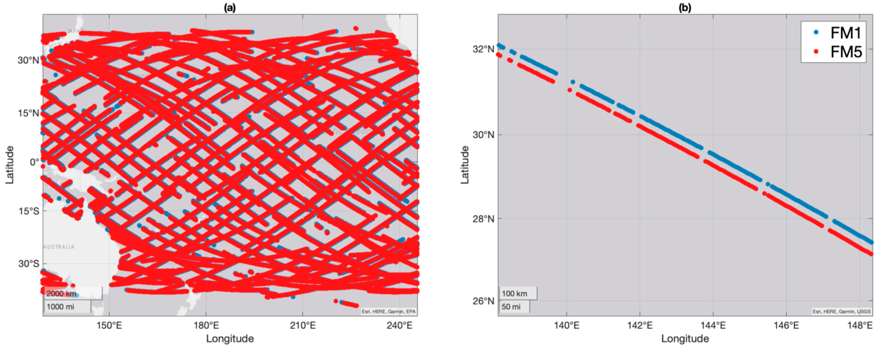
2.3.1. Curating Matchup Observations

As a constellation of eight small satellites in the same orbital plane, CYGNSS is generally unable to collect collocated, near-simultaneous observations from different satellites. If the CYGNSS observatories were equally distributed across the orbital plane, each asset would follow the next at approximately a 10 min lag. However, in that time, both of the uniquely defining features of the CYGNSS observation changes: (1) the surface of the Earth rotates underneath the observatories, changing the ground track, and (2) the GPS satellites that serve as the source of radar signal advance in their orbit. Therefore, in 10 min, it can be quite challenging to develop one-to-one matchup conditions suitable for investigating the correlated error structure at timescales of seconds to minutes.

CYGNSS has no onboard thrusters, and orbit phasing is controlled solely through differential drag. At several junctures during the CYGNSS mission, one of the observatories advanced within the plane to be nearly overlapping with another yet at a slightly different altitude. Generally, the greater the altitude difference between the observatories, the faster the relative precession within the orbit plane.

An exhaustive review of each observatory’s ephemerides for the life of the mission identified a few matchup opportunities. Matchups near the beginning of the mission were preferred, as the orbit planes of the satellites tend to drift apart over the lifetime of the mission. After further filtering by the operational status of each observatory to ensure that they were in similar attitude configurations and operating in similar science modes, a 24 h period starting 0Z on 11 SEP 2019 was chosen, where FM1 and FM5 were in a nearly identical orbital phase for a sustained period. A representation of the ground sampling during this period is shown in Figure 1.

Each ‘track’ of observations (when a series of observations are made in close succession sharing a CYGNSS receiver and GPS transmitter) was matched sample-for-sample between FM1 and FM5 by first minimizing the distance between observations and then quality controlling for several factors:

• Matched tracks must both contain more than 300 samples;
• Individual sample matchups are valid if samples are within 0.5 degrees (great circle distance);
• Individual samples are screened to ensure no quality control flags apply; and
• The matched track is only valid if 60% of the data remains after all other matchup criteria apply.

The resulting matchup conditions produced 103 matched tracks within the 24 h period of near-simultaneous observations.

2.3.2. Generating Model NBRCS

A forward model for the CYGNSS observatory (generating ${\mathsf{\sigma }}_{\mathrm{m}\mathrm{o}\mathrm{d}}^{\mathrm{o}}$ from wind data) can be challenging. Operationally, CYGNSS uses a GMF LUT that maps between the two quantities. However, for the purposes of this analysis, we prefer to use a physically representative forward operator that represents the physical dynamics of the roughening of the ocean surface due to locally driven winds.

For each sample matched up, ${\mathsf{\sigma }}_{\mathrm{m}\mathrm{o}\mathrm{d}}^{\mathrm{o}}$ is generated by computing a spectrally corrected ocean surface MSS from an ERA5-forced [37] WaveWatch III wave model as described in [38]. Because the resolution of ERA5 is much coarser than CYGNSS Level 1 observations in both space and time, the ${\mathsf{\sigma }}_{\mathrm{m}\mathrm{o}\mathrm{d}}^{\mathrm{o}}$ is matched up with ${\mathsf{\sigma }}_{ }^{\mathrm{o}}$ via a tri-linear interpolation across three dimensions (latitude, longitude, and time).

Therefore, for every track of data, there are observations from two different CYGNSS observatories and two modeled NBRCS from reanalysis data.

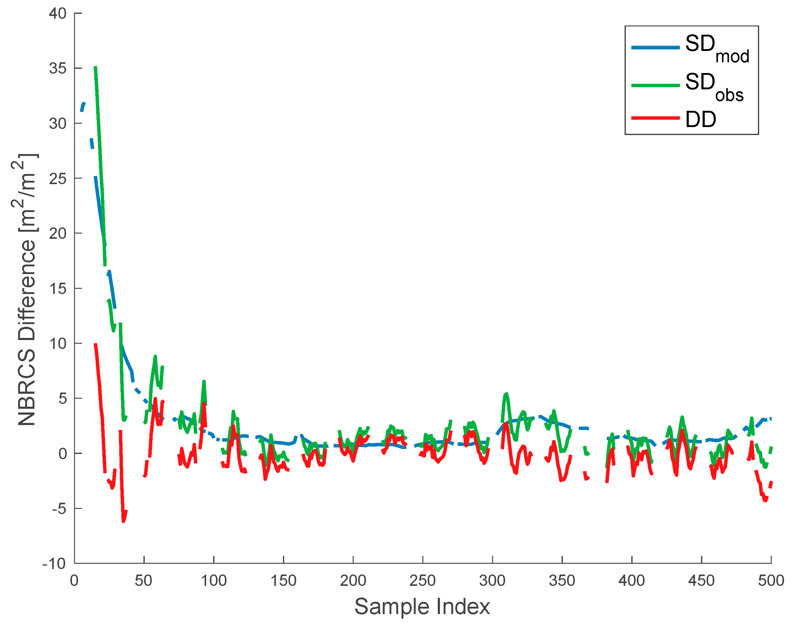
2.3.3. Estimating Total Correlated Error

Single- and double-differencing are common techniques to calibrate remote sensing instruments, especially radiometers [39,40] and radars [41]. Both are useful for quantifying the correlated error structures in CYGNSS observations.

For each track of data, there are two single-differenced datasets,

$$S{D}_{obs}={\sigma }_1^o-{\sigma }_5^o$$

(8a)

$$S{D}_{mod}={\sigma }_{mod,1}^o-{\sigma }_{mod,5}^o$$

(8b)

where $S{D}_{obs}$ is the single-differenced data from the two matched-up observations from FM1 and FM5, and $S{D}_{mod}$ is the single-differenced data of the model-generated NBRCS for the specific coordinates of FM1 and FM5. The double-difference is computed by differencing these two quantities:

$$DD=S{D}_{obs}-S{D}_{mod}$$

(9)

Both the SDs and DD are useful for our analysis. The $S{D}_{obs}$ term represents the difference in ${\sigma }^o$ measured by two different CYGNSS satellites. Despite the strict matchup conditions, these assets are still measuring different fields of view at different times. These differences may result in some residual correlated structure. In addition, any correlated structure in $S{D}_{obs}$ may not reveal structure imposed from fundamental properties of the earth system. Therefore, $S{D}_{mod}$ allows us to identify the correlated structure of any systematic differences in observation target. An example of the utility of these differencing techniques is shown in Figure 2.

Since we are primarily interested in correlated error, and not absolute error, our primary investigative tool is the autocorrelation function. The correlated error for each track can be computed by autocorrelating the DD using the standard formulation:

$$\rho \left(\tau \right)=\frac{1}{(N-\tau )}\frac{1}{{{\sigma }_x}_i}\frac{1}{{{\sigma }_x}_{i+\tau }}\sum _{i=1}^{N-\tau }{(X}_i-\overline{X}){(X}_{i+\tau }-\overline{X})$$

(10)

where $\tau$ is the lag, $N$ is the total number of lags observed, $X_i$ is the value of timeseries $X$ at time $i$, $\overline{X}$ is the mean of timeseries $X$, and the standard deviation is formulated as normal, ${\sigma }_i=\sqrt{\frac{{\sum }_{i=1}^{N-\tau }{(X}_i-\overline{X}{)}^2}{N-\tau }}$.

Because the error correlation behavior can vary from track-to-track, we also construct a bulk autocorrelation which approximates the autocorrelation behavior for all tracks sampled. For this we consolidate $M$ tracks, the bulk autocorrelation is:

$$\mathcal{R}\left(\tau \right)=\frac{1}{M\left(N-\tau \right)}\frac{1}{{{\sigma }_y}_i}\frac{1}{{{\sigma }_y}_{i+\tau }}\sum _{i=1}^{N-\tau }{(Y}_i-\overline{Y}){(Y}_{i+\tau }-\overline{Y})$$

(11)

where $Y_i={\sum }_{j=1}^M{X}_{i,j}$, $j$ is the index for track number, and the standard deviation and mean are calculated as before, but with the consolidated track series $Y$.

2.3.4. Model Tuning

The constructed correlated error model $R_{mod}\left(i,j\right)$ is designed to estimate the correlated error between arbitrary samples $i$ and $j$. Validating the correlated error with empirical matches is challenging since the empirical error correlation can only be estimated in a broader, statistical sense. To create an appropriate comparison, we introduce the modeled error autocorrelation ${\tilde{\rho }}_{mod}$, which is a function of lag $\tau$:

$${\tilde{\rho }}_{mod}\left(\tau \right)=\frac{1}{N-\tau }{\sum }_{i=1}^{N-\tau }{R}_{mod}\left(i,i+\tau \right),$$

(12)

where $R_{mod}$ is calculated using Equation (7), $\tau$ is the lag, and $N$ is the total number of lags observed. The quantity ${\tilde{\rho }}_{mod}$ is reasonably comparable to the autocorrelation $\rho \left(\tau \right)$ of observed error for a single track of samples. A similar analog can be made for the bulk modeled error autocorrelation ${\tilde{\mathcal{R}}}_{mod}\left(\tau \right)$, which estimates the autocorrelation behavior of the error model across M tracks:

$${\tilde{\mathcal{R}}}_{mod}\left(\tau \right)=\frac{1}{M}{\sum }_{j=1}^M{\tilde{\rho }}_{mod,j} \left(\tau \right) ,$$

(13)

where ${\tilde{\rho }}_{mod,j} \left(\tau \right)$ is the modeled autocorrelation for track $j$ at lag $\tau$.

A parametrized version of $R_{mod}$ is constructed using the following form:

$$R_{mod}\left(\alpha ,\beta ,\gamma ,\delta \right){|}_{i,j}=\frac{1}{\mathcal{N}}\left[R_{P^g}\left(\alpha ,\beta \right)+R_{P^Z}\left(\alpha ,\beta \right)+R_{G^R}\left(\gamma ,\delta \right)+R_{G^Z}\left(\gamma ,\delta \right)+R_{\zeta }\left(\beta \right) \right] ,$$

(14)

where the following is true:

• α represents the relative magnitude of the white noise component of the error, which decorrelates at τ = 1;
• β represents the relative magnitude long-decay pedestal or any residual correlated errors at the edge of our timescales of interest;
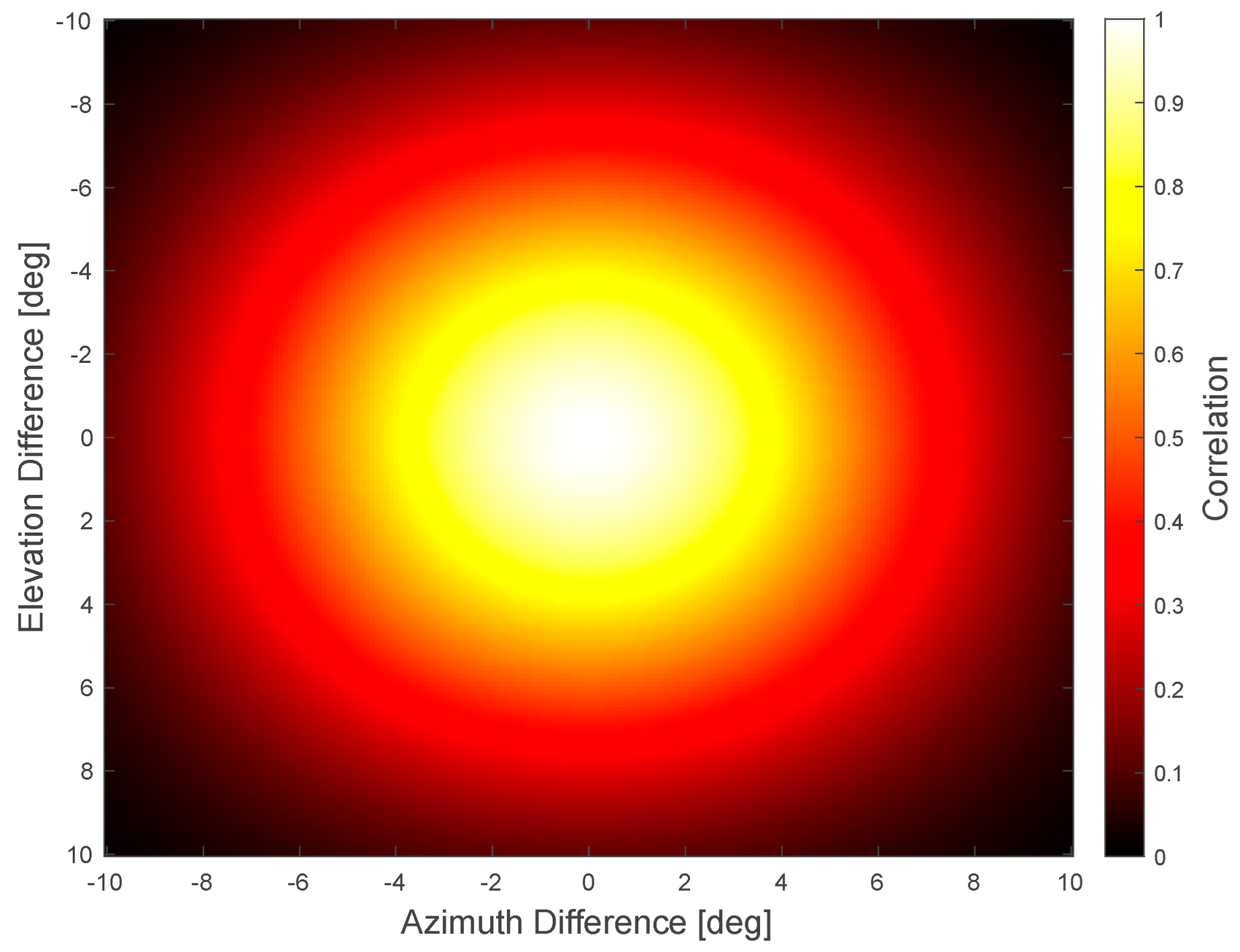
• γ represents the relative magnitude of the correlated error caused by the terms  $R_{G^R}$ and  $R_{G^Z}$, which exhibit smooth decay as samples spread apart when projected through the nadir and zenith antenna coordinates, respectively [see Appendix D for an in-depth discussion]; and
• δ represents the relative decorrelation roll-off in terms $R_{G^R}$ and $R_{G^Z}$.

With an appropriate benchmark, the tuning parameters $\alpha$, $\beta$, $\gamma$, and $\delta$ are iterated such that ${\tilde{\mathcal{R}}}_{mod}$ matches a target signal. The tuning parameters are applied such that they can be modified to change specific characteristics of the modeled behavior:

The parameters modify $R_{mod}$ directly and are described in depth in Appendix B, Appendix C, Appendix D and Appendix E. The target for matching the modeled autocorrelation ${\tilde{\mathcal{R}}}_{mod}$ is the bulk autocorrelation of the double-differenced data DD:

$$\mathcal{R}\left[DD\right]\left(\tau \right)\cong {\tilde{\mathcal{R}}}_{mod}\left(\tau \right)$$

(15)

Because this is an under-determined system, there is no unique solution to optimizing the tuning parameters. Further, these parameters all relate to one another, and changing one will impact the others. Instead, $R_{mod}$ is tuned heuristically such that the modeled behavior matches the empirical data at key points: to match the white noise component at lag $\tau =1$; to match the rolloff at lags $\tau =5$ and $\tau =30$; and to match the endpoint behavior at lag $\tau =100$.

3. Results

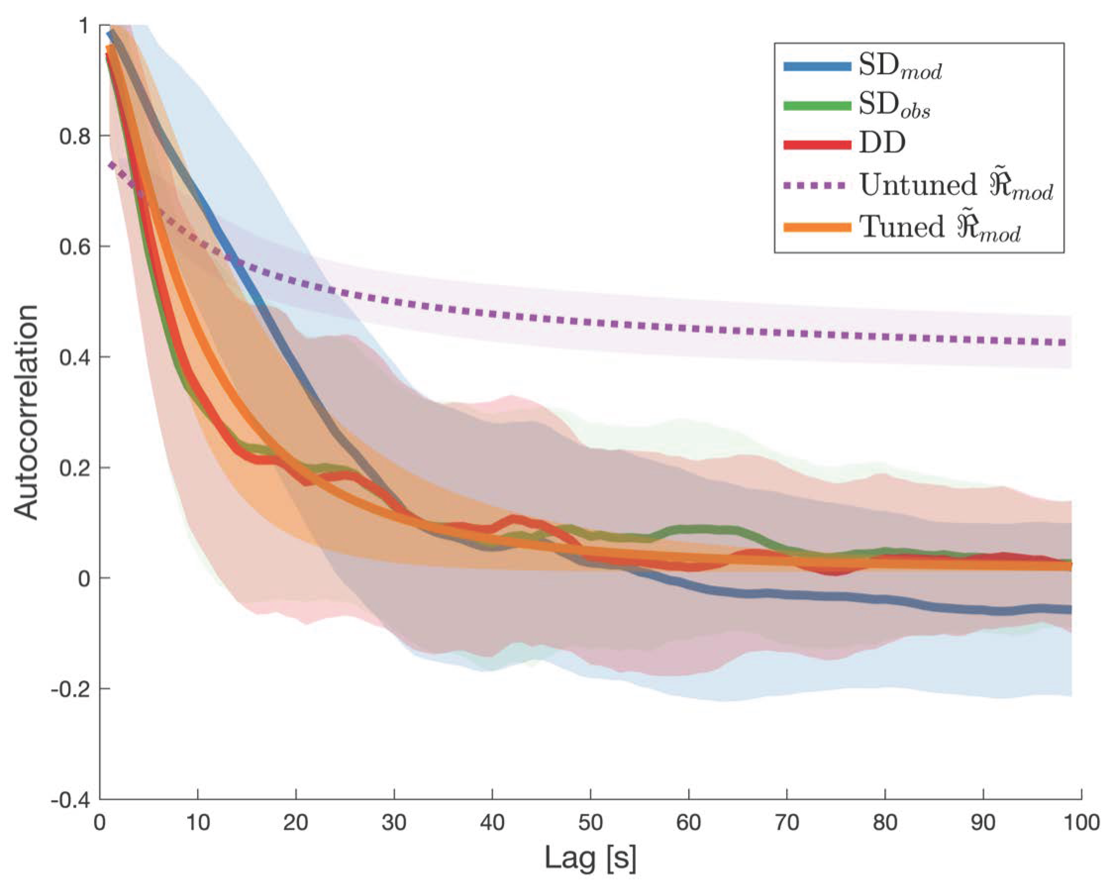
3.1. Bulk Behavior

The constructed model $R_{mod}$ is first tuned to match the overall behavior of $\mathcal{R}\left[DD\right]\left(\tau \right)$, as described in Section 2.3.4. With the appropriate tuning parameters, the bulk-modeled autocorrelation ${\tilde{\mathcal{R}}}_{mod}$ closely resembles $\mathcal{R}\left[DD\right]\left(\tau \right)$ in most important aspects, including the relative magnitude of the white noise component, the relative rate of decorrelation roll-off, and endpoint behavior at large lags. The final tuned ${\tilde{\mathcal{R}}}_{mod}$ is shown in Figure 3 with $\mathcal{R}\left[S{D}_{obs}\right]$, $\mathcal{R}\left[S{D}_{mod}\right]$, and $\mathcal{R}\left[DD\right]$.

The behavior in Figure 3 is worth discussing in detail. The single-differenced model generated ${\sigma }_{mod}^o$ decays at a much slower rate than the single-differenced observations, and double-differenced data suggests that the errors of slight mismatch in observation location and time are generating errors on a fundamentally different scale than the instrument errors. Further, the fact that the double-differenced decorrelation is almost identical to the observation single-differencing suggests that single-differencing near-simultaneous observations are a reasonable approximation for bulk error correlation.

Evaluating the double-difference trace in Figure 3 also reveals important qualities of the CYGNSS error correlation structure. First, the uncorrelated error component accounts for roughly 5% of the total system error. Therefore, assumptions that samples may be treated as independent with uncorrelated error are empirically refuted. Further, the error decorrelation roll-off is swift: about 50% of the error decorrelates within 7 s of observation. Using a flat-plane approximation of Earth, this corresponds to a distance of approximately 50 km, which is generally the scale of the gridding of modern global weather models but much coarser than the resolution of state-of-the-art regional models. Finally, the endpoint behavior at large lag times suggests a small, positive correlated error (~2%) at larger timescales. The statistical properties of the lag correlation become less stable at larger lags, but the existence of a long-timescale correlation is not surprising, considering all observations from a single receiver share a common electronics and processing chain.

The fact that our tuned model $R_{mod}$ can approximate the bulk error correlation structure ${\tilde{\mathcal{R}}}_{mod}$ with similar features as $\mathcal{R}\left[DD\right]$ validates the assumption that the overall instrument-correlated error can be modeled from the fundamental components of the instrument observable: in our case, the radar-range equation (Equation (2)). Further, that $R_{mod}$ can be generated between arbitrary samples suggests that an observation error correlation matrix R can be generated dynamically from first principles given appropriate knowledge about the instrument and retrieval.

The value of the chosen tuning parameters is also worth investigating. The untuned model is defined by having the parameters $\alpha =\beta =\gamma =\delta =1$. Figure 3 demonstrates that the modification of tuning parameters can change the overall model behavior significantly to match observed behavior. Figure 3 further suggests that the untuned $R_{mod}$ generally overestimates both the relative magnitudes of uncorrelated error (i.e., white noise, tuned by $\alpha$) and totally correlated error (i.e., endpoint correlation, tuned by $\beta$). The chosen parameters for tuning are shown in

Table 2. The chosen magnitudes of model tuning parameters for $R_{mod}$.

Tuning Parameter	Magnitude	Function
$\alpha$	0.005	Relative magnitude of uncorrelated error
$\beta$	0.01	Relative magnitude of endpoint correlated error
$\gamma$	1	Relative magnitude of nearby roll-off
$\delta$	1	Steepness of roll-off component

.

The tuning parameter $\gamma$ is used to vary the relative magnitude of the near-sample correlated error roll-off. In our tuned model, this parameter remains at 1. The tuning parameter $\delta$ is used to enhance or reduce the steepness of the roll-off in correlation caused by two observations moving farther apart in the nadir and zenith coordinate systems. If $\delta >1$, it enhances the steepness of decay. The fact that our optimized tuning maintains $\delta =1$ suggests that the filtering theory discussed in Lemma A1 is a reasonable model of decay.

3.2. Single-Track Comparisons

The tuned model can be compared to single-track autocorrelations $\rho \left(\tau \right)$ of matched-sample double-differences using the modeled error autocorrelation ${\tilde{\rho }}_{mod}$ as described in Equation (12). We compare three exemplar tracks in Figure 4.

The single-track autocorrelation behavior shown in Figure 4 is also revealing of the limitations of this work. The single-track error autocorrelation for double-differenced data is highly variable. This may be due to both artifacts in the data (processing, quality control, insufficient data), as well as the real behavior of the observation. It is worth articulating that the autocorrelation of data is generally less stable with smaller datasets and at longer lags. With our quality control parameters, we flag out significant quantities of data, which decreases the stability of autocorrelations from track to track. We further note the difficulty in exploring the dynamics of this behavior in a statistical sense: our aperture of observation where two CYGNSS assets are in a near-overlap condition is quite rare, and as the mission progresses, the orbit planes of the satellites have drifted, making further matchup scenarios less representative. These behaviors may evolve differently day-to-day or as a function of observed wind speed, but the paucity of data in this configuration makes it challenging to establish sufficient baselines to test for significance.

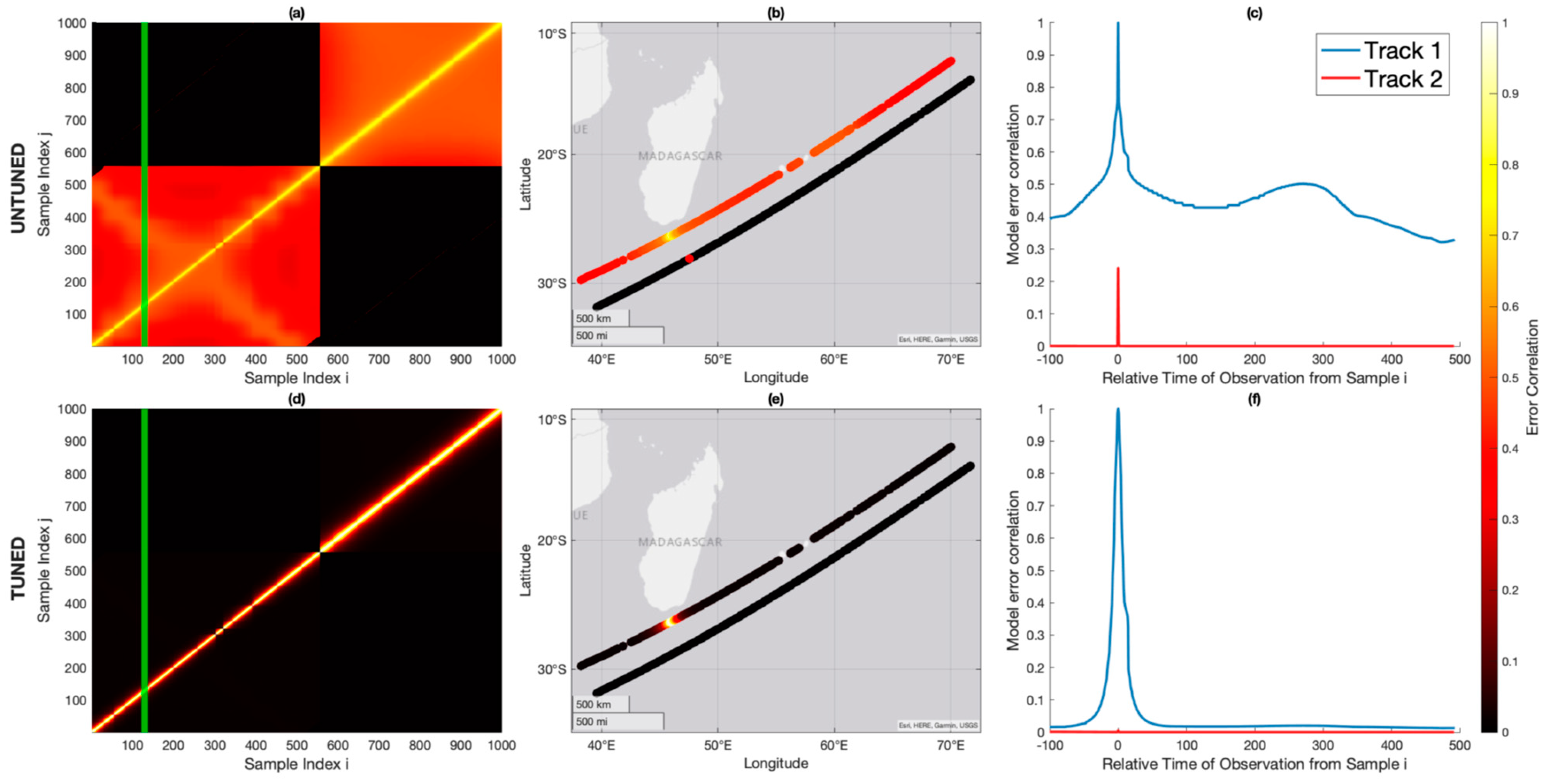
3.3. Dynamic Correlated Error Estimation and Impact of Tuning

The model $R_{mod}$ can produce plausible dynamics, suggesting the broader importance of a realistic dynamic correlated error model. Figure 5 plots two nearby tracks captured nearly simultaneously by the same receiver (but different GPS transmitters).

Because the correlated error $R_{mod}$ can be generated for any arbitrary observation using the bottoms-up model, the dynamics of how instrument errors decorrelate can be explored. To illustrate, we choose an arbitrary exemplar index (i = 129) to demonstrate that this calculation can be performed for any sample within a track. If the observations were treated as completely independent without any correlated error, the matrix in Figure 5a would contain non-zero elements exclusively along the main diagonal. However, we observe several structural elements. The ‘pixelation’ pattern is largely a result of the $R_{\zeta }$ term and originates from the coarse mapping of the estimated GPS antenna gain pattern as a function of scattering incidence ${\theta }_{inc}$. This phenomenon is explored in depth in Appendix D. The smooth decorrelation roll-off is from the $R_{G^R}$ and $R_{G^Z}$ components of the model and represent the direct and reflected signals moving about the nadir and zenith antenna patterns in CYGNSS receivers as the observation is collected along the track. We note that the model allows for cross-track correlation where the two different tracks share a CYGNSS receiver but have a different GPS transmitter. In both the untuned and tuned cases, these tracks appear to have uncorrelated cross-track error. There are residual correlations between the tracks when the scattering geometry is such that the two tracks share similar incidence angles or are near similar antenna coordinates, in addition to the shared receiver noise at lag $\tau =0$.

We can also determine $R_{mod}$ for our matchup tracks where CYGNSS observes similar track geometries with the same GPS transmitter but with two different receivers. The correlated structure for one of the tracks in the previous example (but matched by different receivers) is shown in Figure 6.

The model $R_{mod}$ allows for correlated error between two different receivers that share a GPS transmitter. We note that observations sharing the same GPS transmitter may contain correlated error due to the correlated misestimation of GPS transmit power. This may be an incomplete articulation of the full cross-receiver error correlation. For example, CYGNSS assets in similar orbital regimes may experience similar thermal and environmental conditions that cause correlated errors during our timescales of interest. We assume that correlated error due to misestimation of GPS transmit power is nearly constant for the timescales of interest.

As demonstrated in Figure 6, the cross-track correlation virtually disappears after tuning the model $R_{mod}$. Taken with the data presented in Figure 5, there appears to be negligible cross-track error correlation, either when two tracks share a CYGNSS receiver or when two tracks share a GPS transmitter. This is a novel result but challenging to validate in practice, as the double-differencing may eliminate any shared error correlation between two tracks.

4. Discussion

$R_{mod}$ was designed to maintain several key features. First, $R_{mod}$ can be generated for arbitrary samples in any dataset given the appropriate inputs. Second, $R_{mod}$ is designed to maintain traceability from component error sources with reasonable physical assumptions. Third, $R_{mod}$ is designed to be tuned to allow for calibration and validation as more data becomes available. Finally, $R_{mod}$ is intended to be implementable in a dynamic error model without significant computational expense.

4.1. Limitations

The correlated error model $R_{mod}$ exhibits complex dynamics that are generally plausible but difficult to validate outside of the large-scale statistical estimation discussed in Section 3.1. The fact that the bulk statistical behavior between the estimated autocorrelation model averaged over all tracks is consistent with the observed double-difference autocorrelation (cf. Figure 3) is reassuring, but the disparity between the individual track model estimated autocorrelations and the single-track double-difference estimations (c.f. Figure 4) suggests that either the model is insufficient at capturing the dynamics track-to-track or that the correlated error may not be as stationary as assumed.

With only about a day of data during the overlap period, there remains the possibility that the validation dataset is unrepresentative of the overall statistical behavior of the observation. $R_{mod}$ is designed only to account for errors at short spatial and temporal scales relevant for data assimilation purposes; therefore, this model may not necessarily account for changes of the underlying statistical distributions at larger scales due to seasonality or orbital precession.

The error model assumes that errors are generally isotropic and that $R_{mod}\left(i,j\right)=R_{mod}(j,i)$. This assumption has important practical utility for simplifying the implementation of $R_{mod}$ and the conditioning of the required matrix inversion. Anisotropies may exist in any of the components of the error model but are assumed to be small compared to the modeled behavior.

Further, this model generally assumes no spatial dependence. Spatial dependence of the correlated error is primarily driven by the errors in the retrieval and not the instrumentation, which orbits Earth every 95 min. The ‘spatial’ dependence of error from CYGNSS transiting its orbit has largely to do with the dynamics of the thermal loading of the receiver as lighting conditions evolve in orbit. This is accounted for in the assumptions of the component models $R_{P^g}$ and $R_{P^Z}$ as discussed in Appendix B and Appendix C, respectively. The correlated error resulting from the evolution of the observing geometries as both GPS and CYGNSS propagate in their orbits is captured in the correlated structure of the antenna gain maps and the zenith–specular ratio explored in Appendix D and Appendix E.

4.2. Impact of Tuning Parameters

The application of tuning parameters is a design decision to capture the fact that initial estimates of the bottom’s up error magnitudes may be incomplete and to facilitate rapid adjustments as new calibration and validation information becomes available. The tuning parameters attempt to weigh the value of individual component errors in comparison to each other based on aggregate data from one day of observations during the overlap period.

The specific values of the tuning parameters recovered suggest that the correlated error model $R_{mod}$ overestimates both the uncorrelated and highly correlated components of instrument error. This is useful information for future studies because, as an opportunistic measurement, GNSS-R has limited insight into the error structures in the source signals from GPS.

For observations within a single track, these parameters provide evidence that nearby samples in space and time can add significant new information to a forecast. The tuning parameter $\alpha =0.005$ indicates that the uncorrelated component of the error is significantly overestimated, suggesting that the constituent error magnitudes in [36] may be overestimated. Further, the fact that the tuning parameters $\gamma$ and $\delta =1$ suggest that the overall structure of the error correlation decay is consistent with the theory posited in Appendix D (that the primary source of error correlation is from the application of smoothing filters in the production of antenna gain patterns) and that the application of the Filtering Lemma (Lemma A1) is reasonable.

For observations between tracks, the tuned error model $R_{mod}$ indicates that errors are nearly uncorrelated between tracks (cf. Figure 5 and Figure 6). This is driven primarily by the tuning of the parameter $\beta =0.01$. This has significant practical utility to future assimilation strategies for CYGNSS, suggesting that two nearby tracks are essentially independent measurements with independent instrument error (correlated error may still result from correlated errors in the retrieval or representation).

Finally, it should be noted that the overall effect of the tuning somewhat obviates the need for a dynamic correlated error model, as the overall behavior of the tuned model is quite stable from track to track (cf. Figure 4). This suggests a simplified instrument-correlated error model could be derived from the bulk behavior of ${\tilde{\rho }}_{mod}$, reducing many of the required input data.

5. Conclusions

This work produces a first-principles estimate of correlated instrument error with results that approximate observed statistical behavior. We believe that this model presents a significant advancement in the estimation of the spatial and temporal correlation structure of instrument error for remote sensing systems and, in particular, for the unique considerations of GNSS-R measurements by CYGNSS.

In essence, this work answers a theoretical exercise for enumerating the plausible engineering reasons why two data points from the same observing constellation can share correlated sources of error. We evaluate the correlated error structure for CYGNSS by examining the potential plausible sources of correlated structure from individual components of the instrumentation, combining these sources from first principles as a tuned engineering model, and evaluating the efficacy of the model via a robust validation during a period when two satellites with nearly identical observing geometry captured near-simultaneous and near-collocated samples.

The instrument-originating sources of correlated error is likely to be a small component of the overall correlated structures of observation error. For instance, a likely significant source of correlated error structure is the Geophysical Model Function retrieval that converts observed NBRCS to surface wind speed. These errors can be multifaceted, both encompassing representation error, as the ground truth for training this retrieval is reanalysis data, which may not capture the spatial or temporal dynamics of wind speed [27]. A companion work will explore how the retrieval that maps from NBRCS to wind speed produces correlated error structures in space and time.

Further, the fact that the single-differenced observations generally drive the double-differenced autocorrelation behavior suggests that Powell et al.’s metric of simultaneity and collocation [42] generally applies for CYGNSS when satellites are in a near overlap condition. This interesting result suggests that double-differencing may not be required for statistical estimations of GNSS-R errors given a sufficiently large dataset of observations that nearly overlap. This implication may relax further validation requirements of $R_{mod}$ and may enable near-real-time calibration strategies when samples are sufficiently close without the need to generate reanalysis-driven forward model NBRCS, which introduces significant latencies.

Finally, while the correlated error model $R_{mod}$ was designed to compute the estimated correlated error from arbitrary CYGNSS samples, this may be unnecessary in practice as the tuning makes the model quite stable between samples and tracks. Further, given sufficient assumptions about the stationarity of the instrument-correlated error and the overall magnitude of the instrument-originating sources of correlated error, this information could be conveyed as a static look-up table.

References

- Ruf, C.S.; Chew, C.; Lang, T.; Morris, M.G.; Nave, K.; Ridley, A.; Balasubramaniam, R. A New Paradigm in Earth Environmental Monitoring with the CYGNSS Small Satellite Constellation. Sci. Rep. 2018, 8, 8782. [Google Scholar] [CrossRef] [PubMed]
- Lorenc, A.C.; Ballard, S.P.; Bell, R.S.; Ingleby, N.B.; Andrews, P.L.F.; Barker, D.M.; Bray, J.R.; Clayton, A.M.; Dalby, T.; Li, D.; et al. The Met. Office global three-dimensional variational data assimilation scheme. Q. J. R. Meteorol. Soc. 2000, 126, 2991–3012. [Google Scholar] [CrossRef]
- Bannister, R.N. A review of forecast error covariance statistics in atmospheric variational data assimilation. I: Characteristics and measurements of forecast error covariances. Q. J. R. Meteorol. Soc. 2008, 134, 1951–1970. [Google Scholar] [CrossRef]
- Bannister, R.N. A review of forecast error covariance statistics in atmospheric variational data assimilation. II: Modelling the forecast error covariance statistics. Q. J. R. Meteorol. Soc. 2008, 134, 1971–1996. [Google Scholar] [CrossRef]
- Morss, R.E.; Emanuel, K.A. Influence of added observations on analysis and forecast errors: Results from idealized systems. Q. J. R. Meteorol. Soc. 2002, 128, 285–321. [Google Scholar] [CrossRef]
- Stewart, L.M.; Dance, S.L.; Nichols, N.K. Data assimilation with correlated observation errors: Experiments with a 1-D shallow water model. Tellus A Dyn. Meteorol. Oceanogr. 2013, 65, 19546. [Google Scholar] [CrossRef]
- Fowler, A.M.; Dance, S.L.; Waller, J.A. On the interaction of observation and prior error correlations in data assimilation. Q. J. R. Meteorol. Soc. 2018, 144, 48–62. [Google Scholar] [CrossRef]
- Liu, Z.Q.; Rabier, F. The interaction between model resolution, observation resolution and observation density in data assimilation: A one-dimensional study. Q. J. R. Meteorol. Soc. 2002, 128, 1367–1386. [Google Scholar] [CrossRef]
- Stewart, L.M.; Dance, S.L.; Nichols, N.K.; Eyre, J.R.; Cameron, J. Estimating interchannel observation-error correlations for IASI radiance data in the Met Office system. Q. J. R. Meteorol. Soc. 2014, 140, 1236–1244. [Google Scholar] [CrossRef]
- Bormann, N.; Bonavita, M.; Dragani, R.; Eresmaa, R.; Matricardi, M.; McNally, A. Enhancing the impact of IASI observations through an updated observation-error covariance matrix. Q. J. R. Meteorol. Soc. 2016, 142, 1767–1780. [Google Scholar] [CrossRef]
- Bormann, N.; Bauer, P. Estimates of spatial and interchannel observation-error characteristics for current sounder radiances for numerical weather prediction. I: Methods and application to ATOVS data. Q. J. R. Meteorol. Soc. 2010, 136, 1036–1050. [Google Scholar] [CrossRef]
- Smith, D.; Hunt, S.E.; Etxaluze, M.; Peters, D.; Nightingale, T.; Mittaz, J.; Woolliams, E.R.; Polehampton, E. Traceability of the Sentinel-3 SLSTR Level-1 Infrared Radiometric Processing. Remote Sens. 2021, 13, 374. [Google Scholar] [CrossRef]
- Yang, J.X.; You, Y.; Blackwell, W.; Da, C.; Kalnay, E.; Grassotti, C.; Liu, Q.; Ferraro, R.; Meng, H.; Zou, C.-Z.; et al. SatERR: A Community Error Inventory for Satellite Microwave Observation Error Representation and Uncertainty Quantification. Bull. Am. Meteorol. Soc. 2023, 105, E1–E20. [Google Scholar] [CrossRef]
- Simonin, D.; Waller, J.A.; Ballard, S.P.; Dance, S.L.; Nichols, N.K. A pragmatic strategy for implementing spatially correlated observation errors in an operational system: An application to Doppler radial winds. Q. J. R. Meteorol. Soc. 2019, 145, 2772–2790. [Google Scholar] [CrossRef]
- Waller, J.A.; Dance, S.L.; Nichols, N.K. On diagnosing observation-error statistics with local ensemble data assimilation. Q. J. R. Meteorol. Soc. 2017, 143, 2677–2686. [Google Scholar] [CrossRef]
- Bauer, P.; Buizza, R.; Cardinali, C.; Noël Thépaut, J. Impact of singular-vector-based satellite data thinning on NWP. Q. J. R. Meteorol. Soc. 2011, 137, 286–302. [Google Scholar] [CrossRef]
- Gao, Y.; Xiao, H.; Jiang, D.; Wan, Q.; Chan, P.W.; Hon, K.K.; Deng, G. Impacts of thinning aircraft observations on data assimilation and its prediction during typhoon nida (2016). Atmosphere 2019, 10, 754. [Google Scholar] [CrossRef]
- Hoffman, R.N. The Effect of Thinning and Superobservations in a Simple One-Dimensional Data Analysis with Mischaracterized Error. Mon. Weather Rev. 2018, 146, 1181–1195. [Google Scholar] [CrossRef]
- Rainwater, S.; Bishop, C.H.; Campbell, W.F. The benefits of correlated observation errors for small scales. Q. J. R. Meteorol. Soc. 2015, 141, 3439–3445. [Google Scholar] [CrossRef]
- Stewart, L.M.; Dance, S.L.; Nichols, N.K. Correlated observation errors in data assimilation. Numer. Methods Fluids 2008, 56, 1521–1527. [Google Scholar] [CrossRef]
- Daley, R. The Effect of Serially Correlated Observation and Model Error on Atmospheric Data Assimilation. Mon. Weather Rev. 1992, 120, 164–177. [Google Scholar] [CrossRef]
- Waller, J.A.; Dance, S.L.; Nichols, N.K. Theoretical insight into diagnosing observation error correlations using observation-minus-background and observation-minus-analysis statistics. Quart. J. R. Meteoro. Soc. 2016, 142, 418–431. [Google Scholar] [CrossRef]
- Dee, D.P.; Da Silva, A.M. Maximum-Likelihood Estimation of Forecast and Observation Error Covariance Parameters. Part I: Methodology. Mon. Weather Rev. 1999, 127, 1822–1834. [Google Scholar] [CrossRef]
- Desroziers, G.; Berre, L.; Chapnik, B.; Poli, P. Diagnosis of observation, background and analysis-error statistics in observation space. Q. J. R. Meteorol. Soc. 2005, 131, 3385–3396. [Google Scholar] [CrossRef]
- Ruf, C.; McKague, D.; Posselt, D.J.; Gleason, S.; Clarizia, M.P.; Zavorotny, V.U.; Butler, T.; Redfern, J.; Wells, W.; Morris, M.; et al. CYGNSS Handbook, 2nd ed.; Michigan Publishing Services: Ann Arbor, MI, USA, 2022; ISBN 978-1-60785-787-7. [Google Scholar]
- Clarizia, M.P.; Ruf, C.S. Wind Speed Retrieval Algorithm for the Cyclone Global Navigation Satellite System (CYGNSS) Mission. IEEE Trans. Geosci. Remote Sens. 2016, 54, 4419–4432. [Google Scholar] [CrossRef]
- Ruf, C.S.; Balasubramaniam, R. Development of the CYGNSS Geophysical Model Function for Wind Speed. IEEE J. Sel. Top. Appl. Earth Obs. Remote Sens. 2019, 12, 66–77. [Google Scholar] [CrossRef]
- Gleason, S.; Ruf, C.S.; Orbrien, A.J.; McKague, D.S. The CYGNSS Level 1 Calibration Algorithm and Error Analysis Based on On-Orbit Measurements. IEEE J. Sel. Top. Appl. Earth Obs. Remote Sens. 2019, 12, 37–49. [Google Scholar] [CrossRef]
- Wang, T.; Ruf, C.; McKague, D.; Russel, A.; O’Brien, A.; Gleason, S. The Important Role of Antenna Pattern Characterization in the Absolute Calibration of GNSS-R Measurements. In Proceedings of the 2021 IEEE International Geoscience and Remote Sensing Symposium IGARSS, Brussels, Belgium, 11–16 July 2021; pp. 144–146. [Google Scholar]
- Wang, T.; Ruf, C.; Gleason, S.; McKague, D.; O’Brien, A.; Block, B. Monitoring GPS Eirp for Cygnss Level 1 Calibration. In Proceedings of the IGARSS 2020—2020 IEEE International Geoscience and Remote Sensing Symposium, Waikoloa, HI, USA, 17 February 2020; pp. 6293–6296. [Google Scholar]
- Steigenberger, P.; Thölert, S.; Montenbruck, O. Flex power on GPS Block IIR-M and IIF. GPS Solut. 2019, 23, 8. [Google Scholar] [CrossRef]
- Marquis, W.A.; Reigh, D.L. The GPS Block IIR and IIR-M Broadcast L-band Antenna Panel: Its Pattern and Performance: GPS Block IIR and IIR-M L-band Antenna Panel Pattern. J. Inst. Navig. 2015, 62, 329–347. [Google Scholar] [CrossRef]
- Wang, T.; Ruf, C.S.; Gleason, S.; O’Brien, A.J.; McKague, D.S.; Block, B.P.; Russel, A. Dynamic Calibration of GPS Effective Isotropic Radiated Power for GNSS-Reflectometry Earth Remote Sensing. IEEE Trans. Geosci. Remote Sens. 2021, 60, 1–12. [Google Scholar] [CrossRef]
- Gleason, S. Level 1B DDM Calibration Algorithm Theoritical Basis Document (Rev. 3); University of Michigan: Ann Arbor, MI, USA, 2020. [Google Scholar]
- Powell, C.E.; Ruf, C.S.; Russel, A. An Improved Blackbody Calibration Cadence for CYGNSS. IEEE Trans. Geosci. Remote Sens. 2022, 60, 1–7. [Google Scholar] [CrossRef]
- Gleason, S. Level 1A DDM Calibration Algorithm Theoretical Basis Document (Rev. 2); University of Michigan: Ann Arbor, MI, USA, 2018. [Google Scholar]
- Hersbach, H.; Bell, B.; Berrisford, P.; Hirahara, S.; Horányi, A.; Muñoz-Sabater, J.; Nicolas, J.; Peubey, C.; Radu, R.; Schepers, D.; et al. The ERA5 global reanalysis. Q. J. R. Meteorol. Soc. 2020, 146, 1999–2049. [Google Scholar] [CrossRef]
- Wang, T.; Zavorotny, V.U.; Johnson, J.; Yi, Y.; Ruf, C. Integration of Cygnss Wind and Wave Observations with the Wavewatch III Numerical Model. In Proceedings of the IGARSS 2019—2019 IEEE International Geoscience and Remote Sensing Symposium, Yokohama, Japan, 28 July–2 August 2019; pp. 8350–8353. [Google Scholar]
- Berg, W.; Brown, S.T.; Lim, B.H.; Reising, S.C.; Goncharenko, Y.; Kummerow, C.D.; Gaier, T.C.; Padmanabhan, S. Calibration and Validation of the TEMPEST-D CubeSat Radiometer. IEEE Trans. Geosci. Remote Sens. 2021, 59, 4904–4914. [Google Scholar] [CrossRef]
- Kroodsma, R.A.; McKague, D.S.; Ruf, C.S. Inter-Calibration of Microwave Radiometers Using the Vicarious Cold Calibration Double Difference Method. IEEE J. Sel. Top. Appl. Earth Obs. Remote Sens. 2012, 5, 1006–1013. [Google Scholar] [CrossRef]
- Zec, J.; Jones, W.; Alsabah, R.; Al-Sabbagh, A. RapidScat Cross-Calibration Using the Double Difference Technique. Remote Sens. 2017, 9, 1160. [Google Scholar] [CrossRef]
- Powell, C.E.; Ruf, C.S.; Gleason, S.; Rafkin, S.C.R. Sampled Together: Assessing the Value of Simultaneous Collocated Measurements for Optimal Satellite Configurations. Bull. Am. Meteorol. Soc. 2024, 105, E285–E296. [Google Scholar] [CrossRef]
- CYGNSS CYGNSS Level 1 Science Data Record Version 3.1; NASA: Washington, DC, USA, 2021. [CrossRef]
- Hersbach, H.; Bell, B.; Berrisford, P.; Biavati, G.; Horányi, A.; Muñoz Sabater, J.; Nicolas, J.; Peubey, C.; Radu, R.; Razum, I.; et al. ERA5 Hourly Data on Single Levels from 1940 to Present. Copernicus Climate Change Service (C3S) Climate Data Store (CDS). Available online: https://cds.climate.copernicus.eu/cdsapp#!/dataset/reanalysis-era5-single-levels?tab=overview (accessed on 12 March 2022).
- Taylor, J.R. An Introduction to Error Analysis: The Study of Uncertainties in Physical Measurements, 2nd ed.; University Science Books: Sausalito, CA, USA, 1997; ISBN 978-0-935702-42-2. [Google Scholar]