Abstract
Point cloud registration serves as a critical tool for constructing 3D environmental maps. Both geometric and color information are instrumental in differentiating diverse point features. Specifically, when points appear similar based solely on geometric features, rendering them challenging to distinguish, the color information embedded in the point cloud carries significantly important features. In this study, the colored point cloud is utilized in the FCGCF algorithm, a refined version of the FCGF algorithm, incorporating color information. Moreover, we introduce the PointDSCC method, which amalgamates color consistency from the PointDSC method for outlier removal, thus enhancing registration performance when synergized with other pipeline stages. Comprehensive experiments across diverse datasets reveal that the integration of color information into the registration pipeline markedly surpasses the majority of existing methodologies and demonstrates robust generalizability.
1. Introduction
Rigid point cloud registration, a fundamental task in the fields of computer vision and robotics, involves finding a rigid transformation that aligns two point clouds, which could have many important applications, such as autopilot [1,2,3], surgical navigation [4] and SLAM [5,6]. A commonly adopted registration pipeline typically comprises four consecutive steps: feature detection, feature description, feature matching, and transformation estimation. The effectiveness of a registration algorithm relies on the collaboration of all four components [7]: Feature detection refers to the process of identifying distinctive and salient points or regions within a point cloud model, while the feature description involves capturing and representing the local appearance or characteristics of the detected key points in a compact and informative manner. Then, feature matching is applied to match these descriptors. Finally, the correspondences are used for transformation estimation to find final rigid transformations. It should be noted that the failure of any individual step can result in inaccurate estimation of the transformation, leading to sub-optimal registration performance.
Recent registration studies have been dominated by learning-based methods, most of which establish an end-to-end trainable network, such as [1,8,9] for learning detectors, [10,11,12,13,14] for learning descriptors, [15,16,17] for matching and excluding outliers, and [18,19,20] for transformation estimators. Nevertheless, the presence of repetitive patterns, noise, and uneven point density poses significant challenges in constructing robust models for the aforementioned four components. In particular, for feature detection, the ambiguity of the key point definition may lead to misguidance in the other steps. In the context of description, it is necessary for the acquired descriptors to possess invariance towards unfamiliar rotations. This requirement typically necessitates the utilization of external Local Reference Frames (LRFs) [10,12] or handcrafted rotation-invariant characteristics [21,22]. However, these approaches have limitations in terms of their stability and discrimination ability [13], especially when faced with noise or variations in density. In feature matching, the inaccuracies or deviations that occur during the process of aligning corresponding features in different point clouds can arise due to various factors such as noise, occlusion, incomplete data, or ambiguities in the feature descriptors. For transformation estimation, the presence of repetitive structures or similar local geometric patterns that confuse the algorithm may lead to mismatching when establishing accurate correspondences. To solve this, a Random Sample Consensus (RANSAC) [19], together with other methods [23,24], is utilized to eliminate the outliers.
We argue that all the above challenges can be addressed by utilizing color information. Both geometric and color information play crucial roles in distinguishing different point features. In particular, the color information of the point cloud contains more important features when it is challenging to differentiate points based solely on their geometric features. Ref. [25] emphasized the role of color information in enhancing the registration precision of high point clouds, addressing existing issues with ICP. Similarly, [26] offered a method to impose constraints on both geometric and color information. By leveraging the distribution of color on the tangential plane, a continuous color gradient was established to symbolize the functional shift in color concerning location. A combined error function, comprising geometric and color errors, was developed to effectively restrain both the geometric and color information. However, the employed color space was the RGB color space, which requires the translation of color information into gray-scale information. This process is highly susceptible to disturbances from ambient light, leading to substantial data instabilities. In this study, we investigated the influence of different color spaces on the result when integrating it into the point cloud registration pipeline.
As shown in Figure 1, the colored point clouds were used in the improved FCGF (Fully Convolutional Geometric Feature) and PointDSC (Robust Point Cloud Registration using Deep Spatial) methods with integrated color information for feature extraction and outlier elimination purposes. To evaluate the proposed approaches objectively, a unique colored point cloud dataset based on a forest scene was established. In addition, we developed a strategy for dataset division to create overlapping pairs of colored point clouds for testing. The experimental results demonstrate that the algorithms introduced in this paper can achieve precise point cloud registration by utilizing color and geometric information when cooperating with various ICP methods, even in scenarios with geometric degradation and complex scenes. This proves that the algorithm can enhance the accuracy of colored point cloud registration.
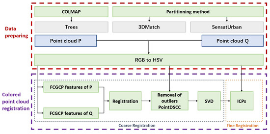
Figure 1.
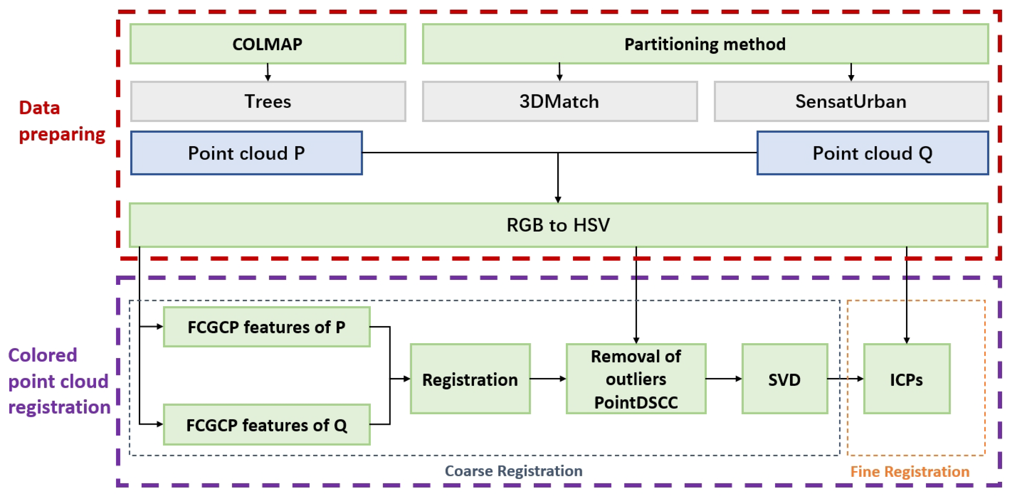
The pipeline of the proposed framework for 3D rigid point cloud registration is as follows. Firstly, the colored point cloud dataset, Trees, is created by COLMAP algorithm. Subsequently, the newly generated dataset Trees, together with other colored datasets 3DMatch and SensatUrban, are divided to overlapping point cloud pairs using a partitioning method proposed in this study. To enhance robustness in varying lighting conditions, the color information is then converted from the RGB format to the HSV color space. Finally, the HSV information is integrated into the improved FCGCF and PointDSCC methods respectively for the coarse registration. This feature is used in the ICP (Iterative closest point) processes as well for the fine registration.
Our main contributions are as follows:
- An improved FCGCF (Fully Convolutional Geometric and Color Feature) algorithm based on FCGF is proposed. This approach incorporates the HSV color information of the colored point cloud into the network. This descriptor is then employed to estimate the correspondences for point cloud registration.
- The PointDSC algorithm is enhanced with the incorporated HSV color consistency among the registration pairs, termed the PointDSCC (Robust Point Cloud Registration using Deep Spatial and Color Consistency). This supports the effective removal of improperly registered point pairings and improves the registration accuracy.
- The creation and partition of datasets. To facilitate the exploration of the algorithms, we created a unique colored point cloud dataset specifically for forest environments. In addition, a dividing method was developed to construct overlapping point cloud pairs from an entire cloud. This not only reduces data storage requirements, but it also enhances computational efficiency and experimental flexibility.
The extensions of the FCGF and PointDSC algorithms, namely FCGCF and PointDSCC, have addressed major issues by incorporating appropriate color information and increasing the dimensionality of consideration. These improvements have expanded the applicability boundaries, enhanced the robustness, and improved the accuracy of point cloud registration pipeline. This improvement is achieved by simultaneously considering both spatial and color consistency aspects.
2. Related Work
For feature extraction, Point Feature Histograms (PFHs) [27] use a parameterized approach to describe the spatial differences between the query point and its neighboring points, generating multi-dimensional statistical histograms to accurately describe the geometric features of the query point. Although PFH can efficiently extract the geometric information of point cloud data, its time complexity is high and the calculation efficiency is low. To solve these problems, researchers proposed the Fast Point Feature Histogram (FPFH) feature descriptor [28]. This feature descriptor improves on the basis of PFHs, introducing the information of the point normal vector, optimizing the calculation process, reducing repeated calculations, and thereby enhancing the calculation efficiency. The FPFH descriptor not only retains all features of the PFH, but it also reduces the time complexity, making it applicable to point cloud data with varying densities or noise levels. Handcrafted point cloud feature descriptors often perform poorly in complex scenarios such as noise and occlusion. However, the rapid development of deep learning in recent years has brought new opportunities for the research of point cloud feature descriptors. Convolutional neural networks have demonstrated remarkable capabilities in deep feature extraction and expression. Therefore, applying deep learning techniques to optimize and replace point cloud feature descriptors has become a mainstream direction in current research.
PointNet [29] uses a simple symmetric function, i.e., max pooling, to handle each point, eliminating the influence of the unordered nature of point cloud data on the output results. However, PointNet has a low sensitivity to local information. To address this issue, PointNet++ [30] was proposed. This network divides the point cloud into local regions and uses PointNet to extract features from each local point cloud, thereby more comprehensively describing local information. Moreover, PointNet++ also employs techniques such as Multi-Scale Grouping (MSG) and Multi-Resolution Grouping (MRG) to handle situations where the point cloud density is uneven, thereby enhancing its robustness. 3DMatch [31] can generate a descriptor for each point in the point cloud data. These descriptors link a point with its surrounding points, thereby providing more comprehensive local information for that point. By comparing the feature descriptors of corresponding points in different point clouds, the 3DMatch network can establish the correspondence between point cloud pairs. A weakly supervised approach is then introduced in 3DFeatNet to learn 3D feature detectors and descriptors. This does not require manually labeled matching point clusters. Instead, for 3D point clouds labeled with the combined GPS/INS (Global Positioning System/Inertial Navigation System), alignment operations and attention mechanisms are used to learn the point features. The Fully Convolutional Network (FCGF) [11] uses sparse convolution in the MinkowskiEngine [32] to replace traditional 3D convolution, thus improving the utilization of space and time. Moreover, the network also designs a loss function using metric learning methods, providing a new perspective for point cloud registration research. The D3Feat network [8] operates by using the Fully Convolutional Network of KPConv [33] and a joint optimization framework to simultaneously detect key points and extract feature descriptors. Additionally, it proposes a new density-invariant key point selection strategy to ensure that the extracted key points can be repeatedly detected.
For feature matching and transformation estimation, a significant portion of traditional methods require an initial transformation, tending to find a locally optimal solution near the starting point. The Iterative Closest Point (ICP) [34], algorithm, an early and notable example, functions through this process. ICP begins with an initial transformation, and then it repeatedly alternates between solving two straightforward sub-problems: identifying the closest points as correspondences under the current transformation, and calculating the optimal transformation using Singular Value Decomposition (SVD) based on the discovered correspondences. Numerous modifications [35,36,37] have been suggested to enhance the ICP methodology. Nonetheless, ICP and its derivatives can merely converge to a local optimum, and their effectiveness heavily dependent on a sound initialization. The misaligned point pairs found based on the extracted feature descriptors will have a negative impact on the registration results; thus, RANSAC-like methods have been introduced to combat this. Fast Global Registration (FGR) [38] optimizes a correspondence-based objective function using a graduated non-convex strategy, achieving cutting-edge results in correspondence-based point cloud registration. PointDSC [24] removes incorrectly registered point pairs based on the principle of spatial consistency, introducing random seeds to alleviate the problem where correct matches fail to dominate when there are many outliers, thereby improving the final registration results. However, these correspondence-based methods can be sensitive to duplicate structures and partial-to-partial point clouds. In such situations, a substantial portion of the potential correspondences might be incorrect.
With advancements in sensor technology, acquiring color information in point clouds has become significantly more accessible, even at low costs. RGB-D cameras [39] combine RGB (color) and depth sensors to capture both color and depth information simultaneously. They are commonly used for indoor 3D scanning and mapping applications. Some LiDAR scanners are equipped with integrated cameras [40] that capture color images alongside the 3D point cloud data. This allows for the acquisition of colored point clouds with precise spatial information. Photogrammetry [41,42] involves capturing a series of overlapping images of a scene from different angles and processing them to reconstruct a 3D point cloud. By capturing high-resolution color images, photogrammetry can generate colored point clouds. Some structured light scanners [43,44] project a pattern of structured light onto the scene and use cameras to capture the deformation of the pattern and color information simultaneously. By analyzing these information, a colored point cloud can be generated. Hence, numerous studies have been put forth aiming to enhance the precision of point cloud registration by integrating color map data. The traditional formulation for integrating color into geometric registration algorithms is to lift the alignment into a higher-dimensional space, parameterized by both position and color [34,45,46,47]. Ref. [48] reduced the impact of ambient brightness changes by converting the RGB color space into a hue color space.
3. The HSV Color Space
In this section, we introduce that the HSV color space is used to express the color information in this study. Typically, the RGB format is a color space that frequently employed due to its composition of three primary colors: red, green, and blue. Each of these colors has a range between 0 and 255, making it a widely utilized model in the field of computer vision. However, the RGB color space presents some challenges; it lacks uniformity, the color differences are not directly proportional to spatial distances, and it doesn’t manage brightness levels well. Moreover, the ambient light can affect the point cloud, causing color deviations when models are taken from different angles.
To solve the aforementioned problem, this article utilizes the HSV color model. The HSV color space is established based on human visual perception, composed of Hue (H), Saturation (S), and Value (V). Among these, V is independent of the point cloud’s color information, while H and S correlate with the way humans perceive color. Using the HSV color space allows for the separation of color and brightness. Setting the red, green, and blue channels in each original RGB point cloud as , and as the largest of the three channels, the formula for transforming the RGB color model to the HSV color model is as follows:
where , respectively, represent the normalized results of R, G, and B in corresponding places; is the minimum value of and ; and is the difference between the maximum value and minimum value of , and .
4. Fully Convolutional Geometric and Color Features
In this section, the HSV information is integrated into the FCGF algorithm, enhancing the robustness and precision of the registration.
4.1. Preliminary
FCGF is a feature extraction algorithm based on learning, utilizing a 3D Fully Convolutional Network. Traditional 3D convolution operations typically need a fixed size for the input data, therefore requiring large-scale point cloud data to be segmented. However, fully convolutional operations can accept inputs of any size, with the output size correspondingly matching the input, hence eliminating the need for data segmentation. Moreover, Fully Convolutional Networks have a large receptive field, allowing them to perceive extensive contextual information; they also possess weight sharing characteristics during training, making them faster and more efficient. A metric learning loss is used for fully convolutional feature learning.
The sparse tensor for 3D data can be represented as a set of coordinates C and associated features F.
Convolutions on sparse tensors (also known as sparse convolutions) require a somewhat different definition from conventional (dense) convolutions. In discrete dense 3D convolution, we extract input features and multiply with a dense kernel matrix. Denote a set of offsets in n-dimensional space by , where K is the kernel size. For example, in 1D, and denotes the kernel value at offset i.
For sparse convolutions, a sparse tensor has a feature at location u only if the corresponding coordinates are present in the set C. Thus, it suffices to evaluate the convolution terms only over a subset . (I.e., the set of offsets i for which is present in the set of coordinates C.) The generalized sparse convolution can be summarized as
where and are the sets of input and output coordinates, respectively, and K is the kernel size.
In FCGF, a U-Net structure with skip connections and residual blocks is implemented to extract such sparse fully convolutional features, and the “hardest contrastive” and “hardest triplet” metric learning losses are computed.
4.2. FCGCF
FCGCF enhances the network input by incorporating the color information of point clouds as the feature matrix F in the network input. The Fully Convolutional Networks fuse color into the extracted point feature descriptors. This results in the acquisition of FCGCF feature descriptors infused with color information. The modified form of the network input is as follows:
5. Robust Point Cloud Registration Using Deep Spatial and Color Consistency
The PointDSC algorithm incorporates correspondences into high-dimensional features through the joint weighting of features and spatial consistency using SCNonlocal. However, colored point clouds not only possess spatial consistency features but also color consistency features, which constrain the relationships between correctly registered point pairs. Based on this, the PointDSCC is proposed.
5.1. Preliminaries
The PointDSC algorithm is a learning-based outlier removal algorithm based on the concept of the SM algorithm (Spectral Matching). Its core idea is to eliminate erroneous outliers based on spatial consistency relationships. It improves upon the issues present in the SM algorithm by initially using geometric feature extraction for the registered point pairs, replacing the length consistency used in SM for spatial consistency calculations. This addresses the issue of insufficient differentiation with length consistency. Additionally, it introduces random seeds to solve the problem of correctly registered points failing to dominate when there are many outliers.
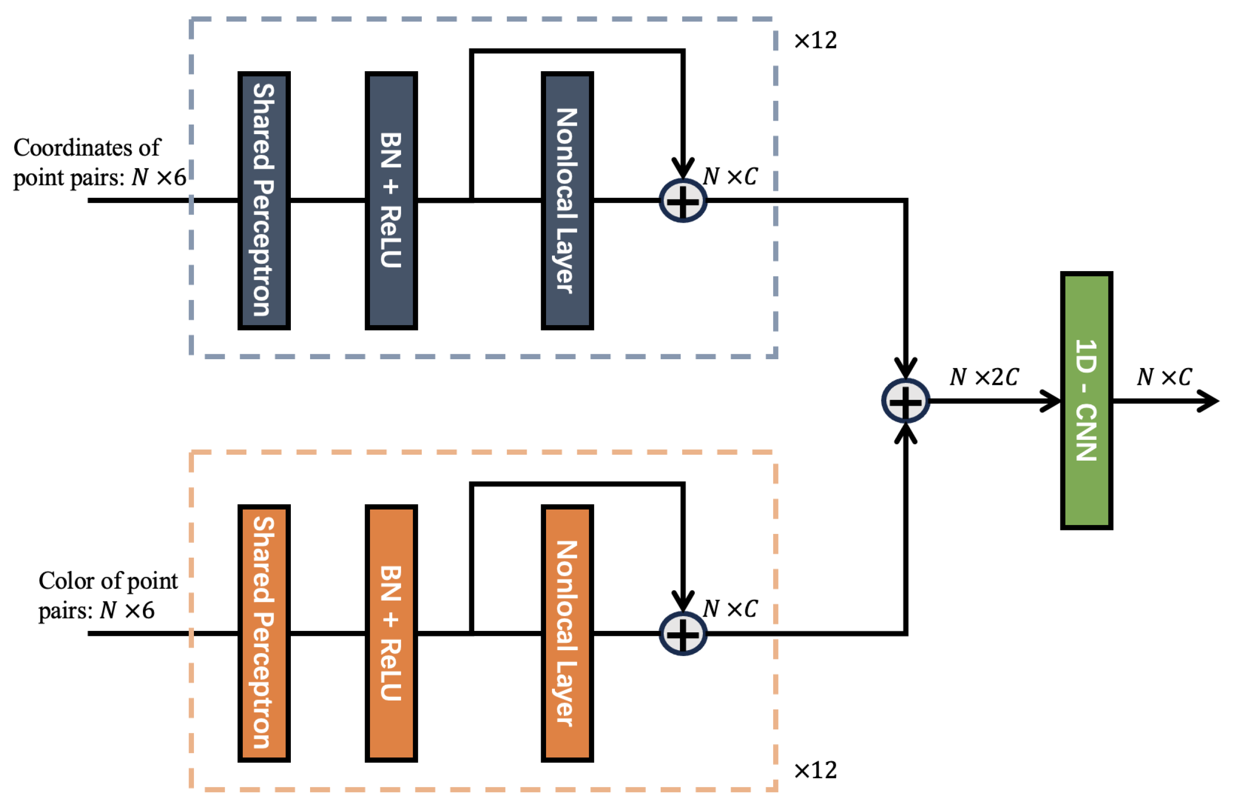
5.1.1. SCNnolocal
First, the input is processed through the SCNonlocal (Spatial Consistency Nonlocal) module to embed correspondences into high-dimensional features, thereby generating a feature for each registered point pair that possess rotation and translation invariance. This module consists of 12 blocks with identical structural parameters, each block consisting of a shared perception layer composed of one-dimensional convolution, a BN (BatchNorm) [49] normalization layer, a ReLU activation layer, and an improved nonlocal layer [50]. The input parameter for this module is a 6-dimensional vector constructed by concatenating the coordinates of each group of registered point pairs , and the output is the high-dimensional feature corresponding to each vector . The feature update formula is as follows:
where g is a linear projection function. The feature similarity term is defined as the embedded dot-product similarity. The spatial consistency term is measured by the length difference between the line segments of the point pairs in and the corresponding segments in . (Multi-layer Perceptron) is utilized to estimate an initial confidence level for each registered point pair, MLP can perform nonlinear transformations and feature extraction on this value.
where is the operation to ensure a non-negative value of , and is a distance parameter to control the sensitivity to the length difference. Correspondence pairs with a length difference exceeding are deemed incompatible and assigned a value of zero. Conversely, assigns a significant value only when the two correspondences, and , exhibit spatial compatibility. This serves as a dependable modulator for the feature similarity term.
5.1.2. Seed Selection
Each feature descriptor extracted by SCNonlocal for every registered pair is fed into a Multi-Layer Perceptron (MLP), which estimates an initial confidence level for each registered point pair. Then, Non-Maximum Suppression [40] is used to obtain multiple local maxima, thereby acquiring uniformly distributed registered point pairs as seeds.
5.1.3. Neural Spectral Matching
For all the seeds obtained, those with higher confidence levels are selected first. Using a nearest neighbor search in the feature space, registration point pairs with similar distances to the seeds in the feature space are clustered, thus expanding each seed into a set of registration point pairs. Each pair set is input into the NMS (Neural Spectral Matching) module, and based on the principle of spatial consistency, the registration point pair sets with higher confidence levels are identified.
5.1.4. Singular Value Decomposition
For each set of registration point pairs, a transformation matrix is obtained through SVD (Singular Value Decomposition). From all the hypotheses, the best transformation matrix is selected, which is the matrix that includes the most correct registration point pairs.
5.2. PointDSCC
As shown in Figure 2, similar to the principle of spatial consistency, the color difference between the correctly registered point pairs should be equal. Based on this principle, the SCNonlocal model is improved in PointDSCC.
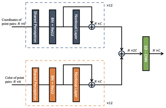
Figure 2.
Improved SCNonlocal(Spatial Consistency Nonlocal) module network structure. Similar to the principle of spatial consistency, the color difference between the correctly registered point pairs should be equal. The consistency coefficient is jointly determined by the spatial and the color consistency coefficient.
In the improved SCNonlocal, the consistency coefficient is jointly determined by the spatial consistency coefficient and the color consistency coefficient .
where indicates the color difference between the line segments of the point pairs in and its corresponding segments in , and is the color distance parameter. can be used to adjust the impact weight of the color and geometric information on the registration. Based on our empirical observations, we consistently set the value of to 0.5 across all our experiments, as this choice has consistently yielded favorable performance outcomes.
In PointDSCC, the loss function consists of two parts, node-wise and edge-wise supervision. The formulas are as follows:
where is used to supervise the registration point pairs predicted by the algorithm, and is used to supervise the transformation matrix predicted by the algorithm. is a hyper-parameter used to balance the two loss functions. Based on our experience, we consistently use in all our experiments, which has consistently yielded good performance. represents the predicted registration point pairs. When point i of the source point cloud and point j of the target point cloud are mutual registration pairs, is 1, otherwise it is 0. represents the actual registration point pairs. denotes the set of predicted registration point pairs that remain as registration point pairs under the actual transformation matrix. The BCE (Binary Cross-Entropy) is calculated with the predicted registration point set to obtain .
6. Creation and Partition of the Datasets
This study used colored point clouds, which are uncommon in public datasets. Most existing point cloud datasets, like KITTI [51], typically consist of colorless point clouds. To carry out the algorithmic research and to apply point cloud registration and stitching techniques to forest scenes, a colored point cloud dataset for forest scenes was created, termed Trees. In addition, it is necessary to process colored point clouds to generate overlapping point cloud pairs. Typically, the storage space for point cloud data is substantial, and storing each point cloud fragment with an overlapping area separately would lead to wastage and redundancy in storage. Therefore, an effective method to reduce storage space utilization is to segment a complete point cloud into multiple point cloud fragments that have overlapping areas with each other.
6.1. Trees Dataset
There are many ways to acquire point cloud data, and the devices used for acquisition vary widely. The simplest method for point cloud acquisition involves using LiDAR to measure the distance from the radar to the object, thereby generating a point cloud. However, the high-precision radar required for this method is expensive and unable to capture the color of objects. Therefore, we used COLMAP, a more cost-effective method, to acquire our point cloud dataset.
Since the forest colored point cloud dataset cannot be directly obtained from public datasets, the Trees forest colored point cloud dataset used in this study was collected through field image acquisition in multiple forest parks, including the Beijing Jufeng National Forest Park and the Beijing Olympic Forest Park. We then used the existing open-source software COLMAP for 3D reconstruction to produce multiple pieces of colored point cloud data, which serve as the real dataset for our experiment.
Both parks are excellent locations for conducting forest scene algorithm experiments and applications, as they boast a wealth of tree species and diverse terrains. The flora in these parks include different types of trees and vegetation, providing a rich set of data and samples for algorithmic research. Additionally, the varied terrains in these parks can simulate different forest environments. Therefore, conducting forest scene algorithm experiments and applications in these parks will provide researchers with more accurate and realistic data, contributing to the improvement of the algorithm’s effectiveness and performance.
The Beijing Jufeng National Forest Park is located at the western end of Beiqing Road in the northwest of Haidian District. The park is situated in a temperate humid monsoon climate zone and belongs to the temperate deciduous broad-leaved forest belt, with a forest coverage rate of up to 96.4%. The highest peak in the park is 1153 m above sea level, and it covers an area of 832.04 hectares. The Beijing Olympic Forest Park is located in the North Fifth Ring Lin Cui Road in Chaoyang District of Beijing. The park covers an area of 680 hectares, dominated by arbor-shrub, with a forest coverage rate of 95.61%.
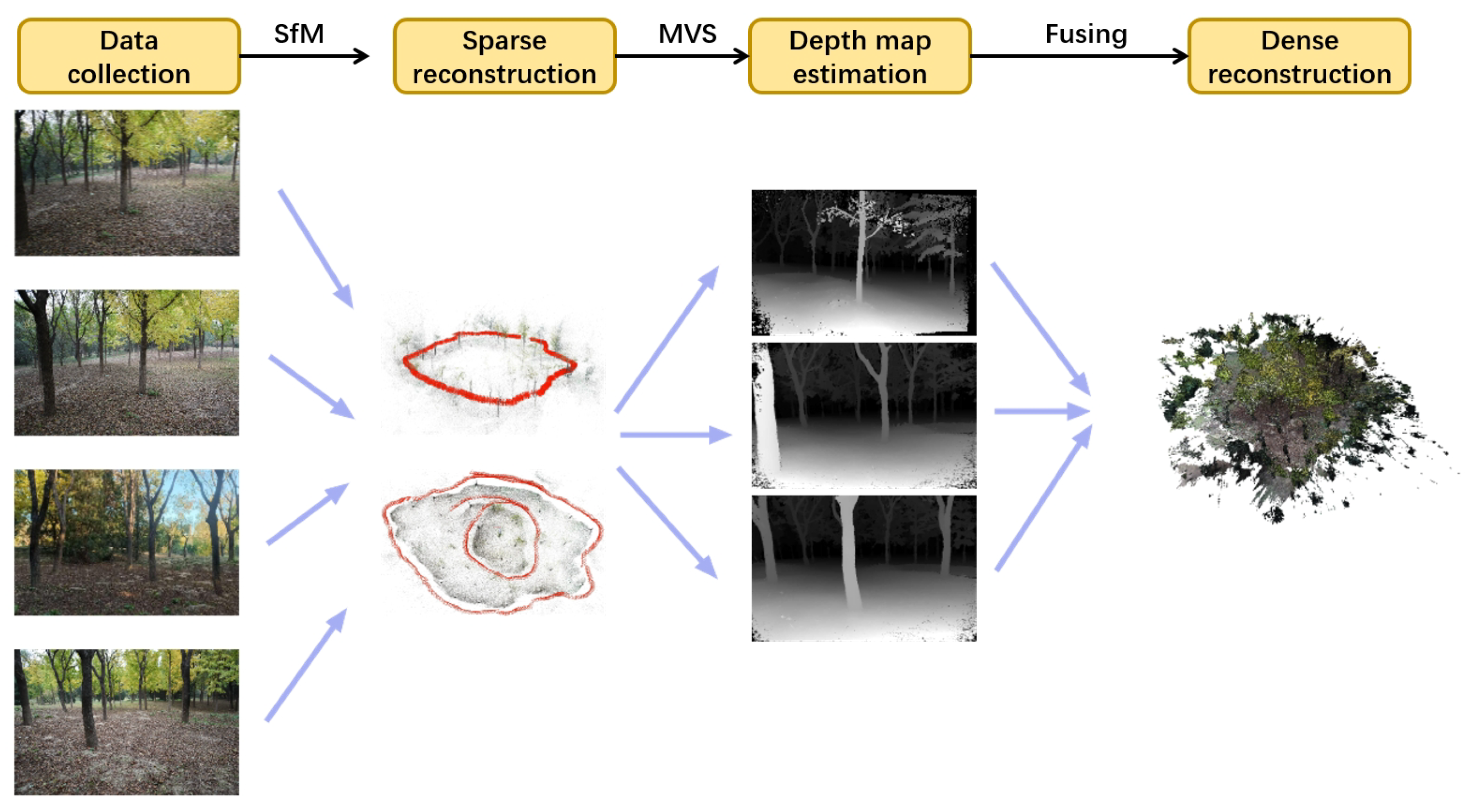
COLMAP utilizes incremental Structure from Motion (SfM) [41] and Multi-View Stereo (MVS) algorithms [42], both capable of reconstructing accurate three-dimensional models from ordered and unordered image collections. The 3D reconstruction process mainly includes the following four steps. Data collection: Gathering a series of high-quality images of the target scene, which can be either ordered or unordered. Sparse reconstruction: This step mainly involves feature extraction and matching on the input images using the SfM algorithm. Depth map estimation: Primarily uses the MVS algorithm to estimate the depth for each input image. Dense reconstruction: Fusing the depth maps into a complete 3D model.
The use of COLMAP for 3D reconstruction does not require depth information of the object, and the captured image dataset can be directly imported into the software to generate a 3D reconstruction model. This makes it a more cost-effective and convenient method compared to other 3D reconstruction approaches. Therefore, as shown in Figure 3, the Trees forest colored point cloud acquisition uses this method.

Figure 3.
Three-dimensional reconstruction of point clouds in the Trees dataset using COLMAP.
Although the point cloud quality of the 3D reconstruction based on COLMAP is not as good as that obtained by LiDAR scanning, the high cost of LiDAR makes it unsuitable for widespread use. In contrast, the point cloud synthesized using the SfM algorithm is less expensive, easier to operate, and still maintains a high level of precision, making it more suitable for experiments.
6.2. Partition Method
In the point cloud partition method we propose, each fragment needs to only store itself and its overlapping neighbors, instead of the entire point cloud data. Then, by combining these segments, a large number of overlapping fragments can be generated for training, validation, and testing. Compared with traditional methods that repetitively store identical point cloud fragments, this approach stores the entire point cloud once as a whole, which can reduce storage space usage while improving computational efficiency and the flexibility of experiments.
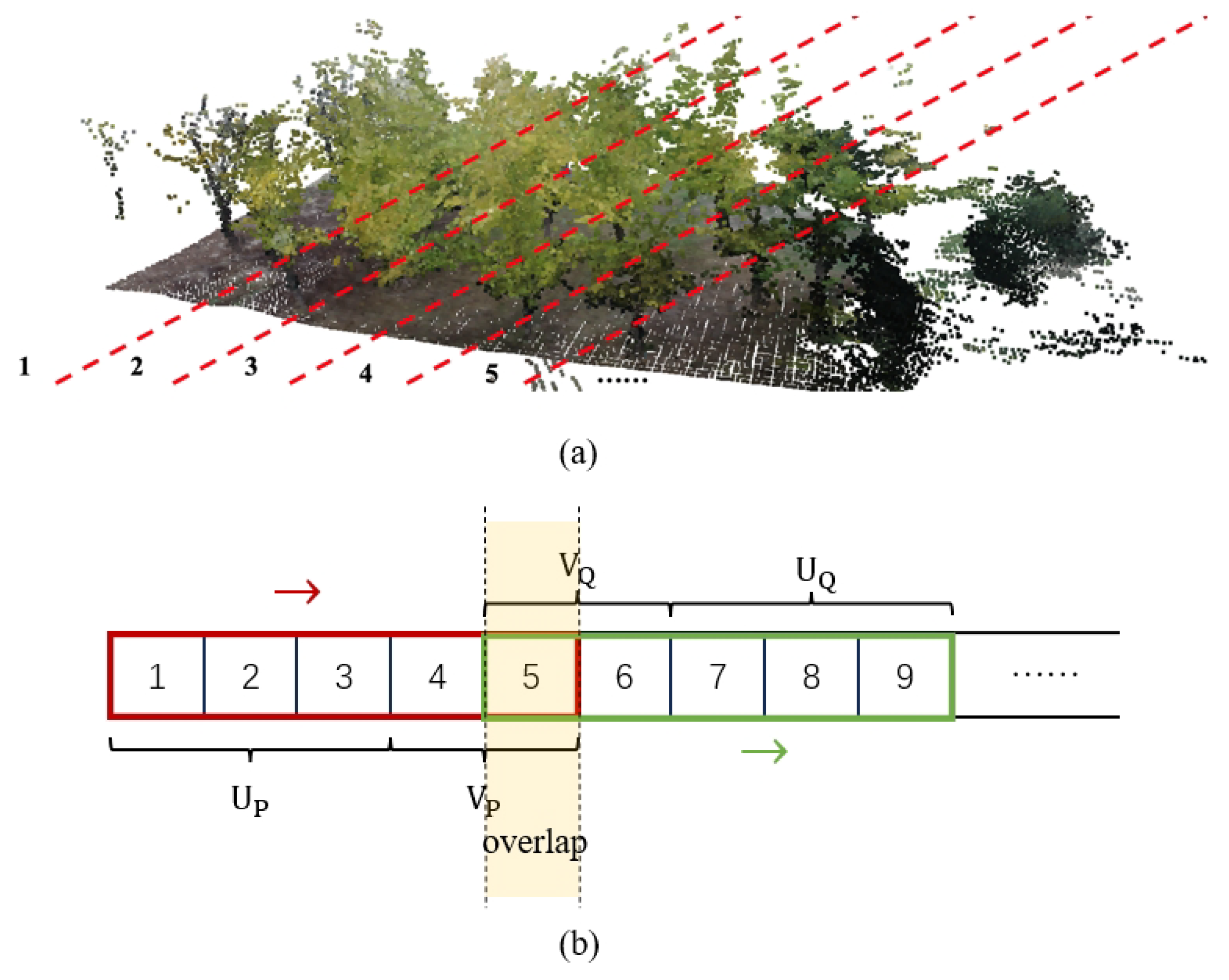
Firstly, in Algorithm 1, a complete point cloud is evenly divided along a certain axis into point cloud fragments numbered from 1 to L, each saved separately, as shown in Figure 4a. Then, the central lengths, and , and the edge lengths, and , of the point clouds, P and Q, are given, respectively. The central length indices and the length of the point cloud fragment indices serve as the main part in one of the point cloud pair, and the edge length refers to the number of indices in the potential overlapping area. Next, these two fragment windows slide from left to right iteratively, consistently maintaining an overlapping portion. After this, to enhance the robustness of the algorithm when faced with noisy situations, we conducted data augmentation on the training dataset to simulate these conditions. Specific measures included (1) randomly dropping 30% of the points in the point cloud; and (2) randomly adding Gaussian noise with a standard deviation of 0.005 to 30% of the points in the point cloud. Finally, when utilizing the point clouds, the selected fragments were combined and stitched together for use, as illustrated in Figure 4b.
| Algorithm 1 The partition method. |
|
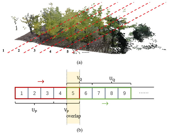
Figure 4.
(a) A complete point cloud is evenly divided along a certain axis into point cloud fragments numbered from 1 to L, each saved separately. (b) The algorithmic process of dividing an entire point cloud into pairs with various overlap rates.
In the above method, we divide each point cloud into multiple non-overlapping point cloud fragments, and then construct overlapping colored point cloud pairs through their flexible combination. At the same time, the augmented point cloud fragments are expect to improve the robustness of the registration. This dataset partition scheme not only effectively reduces storage usage, but it also allows for flexible selection of the overlapping rate between point cloud pairs, enhancing the computational efficiency.
7. Experiments
In this section, we evaluate the performances of FCGCF and PointDSCC and the efficiencies when they cooperate with other steps in the pipeline, including SVD and ICPs. In our experiments, three datasets were used, including Trees, 3DMatch and SensatUrban.
The 3DMatch dataset [31], created by a research team from Princeton University in 2017, is an indoor dataset primarily used for tasks such as point cloud key point detection, point cloud registration, and RGBD image reconstruction. The original 3DMatch dataset does not include point cloud files. Each scene data is composed of two parts: the intrinsic parameters of the camera; and one or more RGB-D video sequence files. Each sequence file contains multiple frames of color images, depth images corresponding to the color images, and text files for the camera pose when the frame was taken. Therefore, it is necessary to synthesize colored point clouds based on the RGB-D video sequence files.
SensatUrban [52,53] is a large-scale urban colored point cloud dataset, encompassing a 7.6 square kilometer range across three cities in the United Kingdom (Birmingham, Cambridge, and York). The dataset includes various categories of geometric structures and landmarks, such as buildings, bridges, railways, sidewalks, etc., and provides color information. This dataset can be used for tasks such as semantic recognition, object recognition, and point cloud registration. Due to the dense point clouds provided by the dataset requiring a significant amount of GPU space and slow computation speed, the performance of algorithm training is impacted. To address this issue, the dataset was sub-sampled using a 0.01 m voxel filter, replacing the points near the center in the voxel grid with all the point clouds within the voxel. This method can reduce the amount of data while maintaining the shape features of the point cloud, consequently not affecting the registration results of the point cloud.
The hardware setup for the experiments included CPU, Intel(R) Core(TM) i5-9500 cpu @ 3.00 GHz; GPU, a single RTX3090Ti; the total device memory was 32 G, and the GPU memory was 24 G. All experiments were conducted in this environment.
7.1. The Results of the FCGCF
7.1.1. Estimating Point Cloud Registration Pair Sets through a Nearest Neighbor Search in the Feature Space
Point cloud feature descriptors exhibit rotation invariance, meaning that the feature descriptors extracted for each point in the point cloud remain unchanged regardless of how the point cloud undergoes rigid transformations. In practical situations, registration pairs of points that have overlap or are extremely close usually possess similar or identical features. Therefore, the distances between these pairs in the feature space are also very close. This allows the use of a nearest neighbor search in the feature space to effectively find registration pairs between each pair of point clouds. That is, for each point in point cloud P, the point in point cloud Q nearest in the feature space can be found as its registration point. The formula for finding the registration points is as follows:
where represents the feature descriptor of point p in point cloud P, and represents the feature descriptor of point q in point cloud Q. is the estimated registration point for point p in point cloud P.
7.1.2. Evaluation Metrics
We use three standard metrics to measure the quality of features under registration: feature-match recall, registration recall, and relative rotation error.
Feature-match recall. The feature-match recall (FMR) [21], measures the percentage of fragment pairs that can recover the pose with high confidence. Mathematically, it is write as
where M is the number of fragment pairs, is a set of correspondences between a fragment pair s, and are 3D coordinates from the first and second fragment, respectively, and is the ground truth pose. is the inlier distance threshold, and or 5% is the inlier recall threshold.
Registration recall. The feature-match recall assesses the performance of features under pairwise registration. Yet, this metric does not evaluate the efficacy of the feature within a reconstruction system. Alternatively, the registration recall [54] operates by considering a group of overlapping fragments with an established ground truth pose, and then it gauges the number of overlapping fragments a matching algorithm is capable of accurately retrieving. Specifically, the registration recall uses the following error metric between the estimated fragments and the corresponding pose estimation to define a true positive.
where is a set of corresponding ground truth pairs in fragments , and and are the 3D coordinates of the ground truth pair. For fragments with at least 30% overlap, the registration is evaluated as a correct pair if [11,17,55]. As noted in several works [21,22,54,56], recall is more important than precision since it is possible to improve precision with better pruning.
Relative translation and rotation error. The feature registration inaccuracies for RANSAC are quantified by the relative translation error (TE), relative rotation error (RE) and the final relative rotation (RR). They are indirect measures. TE and RR are defined as , where is the estimated translation after registration, and , where is the estimated rotation matrix and is the ground truth rotation matrix. When is less than 15° and is less than 30 cm, the registration is considered successful; otherwise, the registration is considered unsuccessful. Therefore, the final calculation formula for RR is .
7.1.3. Training and Testing
The three colored point cloud datasets were used in our experiments. The degree of overlap between the point cloud registration pairs is equal to or greater than 30%. The 3DMatch dataset includes a total of 1295 pairs of test point cloud fragments, the SensatUrban dataset includes 675 pairs, and the forest colored point cloud dataset includes 950 pairs. Each of the dataset is divided into testing, training, and validation datasets randomly, accounting for 20%, 60%, and 20% of the total dataset respectively.The method of adding noise to the datasets is as following: firstly, 30% of the points are randomly discarded, and then Gaussian noise with a standard deviation of 0.005 is added to a random 30% of the remaining points.
We trained and tested the FCGCF feature extraction network under both noisy and noise-free conditions. We compared it with traditional methods, such as FPFH and FCGF point cloud feature descriptors, to evaluate whether the FCGCF feature extraction descriptor has a better performance and stronger robustness in point cloud registration. To ensure the consistency of the experimental environment, we used the same training parameters to train the network model. Specifically, we used the SGD optimizer to optimize the network and set the initial learning rate to 0.1, which gradually decreased as the number of training iterations increased. We used a batch size of four for training and set the batch size to one during the validation process. The maximum number of iterations was set to 100. We also set a judgment criterion, which is an Euclidean distance threshold of 0.1 m between correctly registered point pairs.
7.1.4. Results
Different feature descriptor extraction algorithms were evaluated. To test the robustness of the feature descriptors, experiments were conducted in both noise-free and noisy environments to evaluate the noise resistance of the feature descriptors.
According to Table 1 and Table 2, (In all subsequent tables, an ascending arrow (↑) denotes that larger numerical values correlate with superior performance, while a descending arrow (↓) implies that smaller values are more desirable. The bolded figures within each comparison highlight the optimal outcomes achieved. This convention is uniformly maintained throughout the paper.) for the FCGCF point cloud feature descriptor that included color information, there is a noticeable improvement across the different datasets compared to the FCGF feature descriptor. Compared to FCGF, FCGCF(HSV) in a noise-free environment showed increases of 0.0336, 0.0517, and 0.061 in the FMR (Feature-match recall) metric on the Trees, 3DMatch, and SensatUrban datasets, respectively. In a noisy environment, the FCGCF showed even more significant improvements over the FCGF, exhibiting a better resistance to noise with FMR (Feature-match recall)increases of 0.1611, 0.1098, and 0.1828 on the Trees, 3DMatch, and SensatUrban datasets, respectively. To a certain extent, the RR metric represents the quality of point cloud registration. When analyzing this index, it is important to consider the characteristics of the datasets being used. The SensatUrban dataset consists of large-scale urban-level point clouds, while the Trees and 3DMatch datasets represent point cloud models of scenes within limited ranges and indoor environments. In the large-scale situation, the information is scattered, which may give the impression that the point cloud has a high degree of overlap. However, in reality, a large portion of the point cloud consists of empty regions, and only a small fraction contains truly valuable information. When we apply the same method and parameters to introduce noise, the original point cloud model of the SensatUrban dataset can be significantly disturbed. In addition, the 3D point clouds in the dataset are generated from high-quality aerial images, which may result in lower overlap in certain areas. Therefore, we can expect a significant decrease in the RR metric of the SensatUrban dataset in the presence of noise.

Table 1.
Comparison of the feature extraction algorithms in a noise-free environment.
Table 2.
Comparison of the feature extraction algorithms in a noisy environment.
Comparing the FCGCF feature descriptors extracted with the different color models in a noise-free environment, the FCGCF feature descriptor extracted with the HSV color model did not perform as well as the FCGCF feature descriptor extracted with the RGB color model on the 3DMatch and SensatUrban datasets. However, in a noisy environment, the FCGCF feature descriptor extracted with the HSV color model performed better than the FCGCF feature descriptor extracted with the RGB color model, suggesting that the FCGCF feature descriptor extracted with the HSV color model is more robust. The reason for the advantages of HSV format lies in its resilience to variations in lighting conditions and its close alignment with human perception and description of colors, leading to a more consistent color perception.
7.1.5. Visualization of Features
To intuitively analyze the advantages of the FCGCF(HSV) feature descriptor compared to the FCGF feature descriptor and FCGCF(RGB), Figure 5 exhibits the feature mapping of the point cloud in the SensatUrban dataset with similar geometric information and different color information.This demonstrates the effectiveness of FCGCF(HSV) when the distinction of geometric features is not pronounced. We used t-Distributed Stochastic Neighbor Embedding (t-SNE) [57] to project all features extracted by the different algorithms in the same point cloud onto a color-coded one-dimensional space and visualized them.
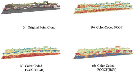
Figure 5.
Color-coded features overlaid on the same point cloud. The features extracted by the different methods are mapped onto a scalar space using t-SNE and colorized with the spectral color map.
As illustrated in Figure 5, the original point cloud is from red and white painted roadblocks in the SensatUrban dataset, where the red and white sections have similar geometric information but different color information. As can be intuitively seen from the figure, both the FCGCF(HSV) and FCGCF(RGB) feature descriptors can clearly distinguish between the two sections, while the FCGF feature descriptor cannot. Moreover, the FCGCF(HSV) feature descriptor clearly distinguishes the puddle next to the roadblock, which FCGCF(RGB) does not, thus demonstrating the superior performance of FCGCF(HSV). When faced with scenes that have similar geometric information but different color information, the FCGCF(HSV) feature descriptor can significantly improve the effect of point cloud registration.
7.2. The Results of PointDSCC
7.2.1. Evaluation Metrics
Following [58], we used seven evaluation metrics, namely (1) registration recall (RR), rotation error (RE), translation error (TE), root mean square error (RMSE), inlier precision (IP), inlier recall (IR) and inlier F1 (F1). The TE (Translation Error) and RR (Registration Recall) are the same as the ones in FCGCF. The IP, IR and F1 are given below as follows:
7.2.2. Training and Testing
We followed the same evaluation protocols in FCGCF to prepare the training and testing data. The ADAM optimizer was used to optimize the network, with an initial learning rate set at 0.0001, which gradually decreased as the number of training iterations increased. Due to the constraints of memory size, the batch size for both training and validation processes was set to 16, and the maximum number of iterations was set to 100. The Euclidean distance threshold between the correctly registered point pairs was set to 0.1 m. To accelerate training, different types of feature descriptors in the dataset were extracted and recorded in advance to avoid re-extracting features from the point cloud during each training session. In the input registration point pairs, only the top 1000 pairs with the closest distance in the feature space were selected. The random seed was set to 10% of the input registration point pairs.
7.2.3. Results
Comparison of the Effects of Different Outlier Removal Algorithms
We compared several outlier removal algorithms, including RANSAC(1000), RANSAC (5000) [19], SM [23], FGR (Fast global Registration) [38], PointDSC [24], and PointDSCC. Since all the tested outlier removal algorithms perform well in a noise-free environment, it is not possible to compare their performance differences. Therefore, in this experiment, we extracted FCGCF(HSV) and FCGF feature descriptors from three noisy datasets and used these descriptors to estimate the initial registration point pairs. In this article, the integration of the HSV color space into the point cloud registration pipeline is proposed. Based on the previous experience, this color space has shown better robustness. Therefore, the RGB format is not considered in other stages of the pipeline. Since each pair of point clouds may have different numbers of correspondences, we randomly sample 1,000 correspondences from each pair to build the batched input during training. Extending the selection beyond 1000 pairs may result in increased time consumption without adversely affecting the actual performance of outlier removal. The comparison results are shown in Table 3, Table 4 and Table 5.
Table 3.
Comparison of the outlier removal algorithms for Trees.
Table 4.
Comparison of the outlier removal algorithms for 3DMatch.
Table 5.
Comparison of the outlier removal algorithms for SensatUrban.
The experimental results show that the registration performance of the algorithm tested on registration point pairs estimated by the FCGCF(HSV) feature descriptor far exceeds that of the algorithm tested on registration point pairs estimated by the FCGCF feature descriptor in all three datasets. This clearly demonstrates the important role of color information in point cloud registration.
For the comparative experiments of different outlier algorithms tested on the registration point pairs estimated by the FCGCF feature descriptor, the proposed PointDSCC algorithm achieved the best results on the RE, TE, IR, and F1 metrics in the 3DMatch dataset. It was slightly lower than the PointDSC algorithm on the RR metric, slightly lower than the SM algorithm (Spectral matching) on the IP metric, and slightly lower than the FGR (Fast Global Registration) and SM algorithms on the RMSE metric.
In the SensatUrban dataset, the PointDSCC algorithm achieved the best scores in the RR, TE, IP, and F1 metrics, but it did not have a clear advantage in the RE, IR, and RMSE metrics.
In the Trees dataset, the PointDSCC algorithm achieved the best scores in the RR, TE, IR, IP, and F1 metrics, but it did not have a clear advantage in the RE and RMSE metrics.
Comparison of Different Fine Registration Algorithms
We performed further registration of the point cloud using a nearest neighbor search and its variant algorithms, including ICP [34], Generalized ICP [59], and Colored ICP [26]. The results on the three datasets are shown in Table 6, Table 7 and Table 8.
Table 6.
Comparison of the Trees dataset fine registration algorithms.
Table 7.
Comparison of the 3DMatch dataset fine registration algorithms.
Table 8.
Comparison of the SensatUrban dataset fine registration algorithms.
The experimental results show that optimizing the registration results further using the nearest neighbor search algorithm can effectively improve the registration effect. Among the three ICP algorithms, the Generalized ICP algorithm performed the best, achieving the best results in most cases. The Colored ICP algorithm only achieved the best results in a very few cases and did not have a clear advantage. Therefore, based on the analysis, the Generalized ICP algorithm has the best accuracy and universality among the three ICP algorithms.
7.2.4. The Display of Outlier Removal Algorithm Effects
To compare the outlier removal effects of different outlier algorithms, different outlier removal algorithms were used for comparison, and the outlier removal results and registration results were visualized. The input still used the registration point pairs extracted from the above-mentioned point cloud using the FCGCF(HSV) feature descriptor, and 2000 pairs were randomly selected as the input. The comparison effect is shown in Figure 6.
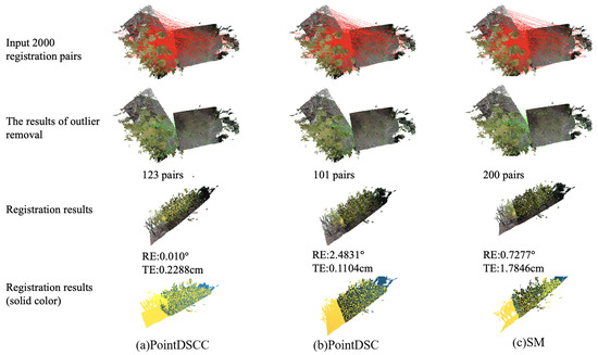
Figure 6.
A comparison of the outlier removal algorithms’ effects.
According to the experimental results, all three point cloud registration algorithms can achieve registration effects with a rotation error less than 15 degrees and a translation error less than 30 cm. However, it is impossible to judge the quality of the algorithm with the naked eye, so rotation error and translation error were used as quantitative evaluation indicators. When using the estimated 2000 registration point pairs extracted using the FCGCF(HSV) feature descriptor as the input, the PointDSCC outlier removal algorithm successfully removed outliers, leaving 123 point pairs. Although the number of outliers removed by the PointDSCC outlier removal algorithm was less than that of the PointDSC algorithm, the PointDSCC outlier removal algorithm achieved the best registration effect among the three algorithms. The quantity of removed outliers, which is related to the quality of both point clouds and the previous stages of the pipeline, is not a crucial factor. Instead, what truly matters is whether the application of the outlier removal algorithm leads to improved performance in the registration results. The registration results in solid color(yellow and blue) could provide a visual representation of the alignment process and the quality of the registration by comparing the colors of corresponding points in the aligned point clouds, discrepancies or misalignments can be easily identified. This finding demonstrates that employing dual constraints based on both spatial consistency and color consistency not only increases the probability of eliminating outliers lacking color consistency but also enhances the likelihood of retaining registration point pairs with weak spatial consistency features yet strong color consistency features.
8. Conclusions
This study presents advancements in color-based registration techniques by integrating colored point cloud data into the FCGCF algorithm. The utilization of the HSV color model allows for the separation of color and brightness components, resulting in a more robust registration process. Additionally, the proposed PointDSCC method incorporates color consistency within the PointDSC framework to identify and eliminate outlier points, improving registration performance and providing insights into color variations within the point cloud data. A specialized colored point cloud dataset for forest environments was curated, along with a partitioning approach to generate overlapping point cloud pairs, optimizing computational efficiency and facilitating more effective registration analysis. Extensive experiments demonstrated the superiority of integrating HSV color information, emphasizing the importance and potential advantages of utilizing color cues in registration processes. This study contributes valuable insights and advancements in color-based registration techniques, with potential benefits for researchers in the field. Our code and the Trees dataset can be made available upon request.
Author Contributions
Methodology, T.H. and R.Z.; software, T.H. and R.Z.; validation, J.K. and R.D.; writing—original draft preparation, T.H.; writing—review and editing, T.H.; visualization, X.Z.; supervision, S.Y.; funding acquisition, J.K. All authors have read and agreed to the published version of the manuscript.
Funding
This work was supported by the National Natural Science Foundation of China (No. 32071680), the National Natural Science Foundation of China (No. 62203059), and the Beijing Natural Science Foundation (No. 6232029).
Data Availability Statement
[3DMatch] Andy Zeng. 2016. 3DMatch: Learning Local Geometric Descriptors from RGB-D Reconstructions; https://3dmatch.cs.princeton.edu/, accessed on 17 January 2022; [SensatUrban] Qingyong Hu. 2022. Sensaturban: Learning semantics from urban-scale photogram- metric point clouds; https://github.com/QingyongHu/SensatUrban?tab=readme-ov-file (accessed on 17 January 2022); Our code and the Trees dataset can be made available upon request.
Acknowledgments
We extend our gratitude to the editor and the anonymous peer reviewers whose constructive feedback and insights have significantly contributed to the enhancement of this paper’s quality.
Conflicts of Interest
The authors declare no conflict of interest.
References
- Li, J.; Lee, G.H. Usip: Unsupervised stable interest point detection from 3d point clouds. In Proceedings of the IEEE/CVF International Conference on Computer Vision, Seoul, Republic of Korea, 27 October–2 November 2019; pp. 361–370. [Google Scholar]
- Li, Y.; Ma, L.; Zhong, Z.; Liu, F.; Chapman, M.A.; Cao, D.; Li, J. Deep learning for lidar point clouds in autonomous driving: A review. IEEE Trans. Neural Netw. Learn. Syst. 2020, 32, 3412–3432. [Google Scholar] [CrossRef] [PubMed]
- Wan, G.; Yang, X.; Cai, R.; Li, H.; Zhou, Y.; Wang, H.; Song, S. Robust and precise vehicle localization based on multi-sensor fusion in diverse city scenes. In Proceedings of the 2018 IEEE International Conference on Robotics and Automation (ICRA), Brisbane, QLD, Australia, 21–25 May 2018; pp. 4670–4677. [Google Scholar]
- Yoo, H.; Choi, A.; Mun, J.H. Acquisition of point cloud in CT image space to improve accuracy of surface registration: Application to neurosurgical navigation system. J. Mech. Sci. Technol. 2020, 34, 2667–2677. [Google Scholar] [CrossRef]
- Han, L.; Xu, L.; Bobkov, D.; Steinbach, E.; Fang, L. Real-time global registration for globally consistent rgb-d slam. IEEE Trans. Robot. 2019, 35, 498–508. [Google Scholar] [CrossRef]
- Deschaud, J.E. IMLS-SLAM: Scan-to-model matching based on 3D data. In Proceedings of the 2018 IEEE International Conference on Robotics and Automation (ICRA), Brisbane, QLD, Australia, 21–25 May 2018; pp. 2480–2485. [Google Scholar]
- Dong, Z.; Liang, F.; Yang, B.; Xu, Y.; Zang, Y.; Li, J.; Wang, Y.; Dai, W.; Fan, H.; Hyyppä, J.; et al. Registration of large-scale terrestrial laser scanner point clouds: A review and benchmark. ISPRS J. Photogramm. Remote Sens. 2020, 163, 327–342. [Google Scholar] [CrossRef]
- Bai, X.; Luo, Z.; Zhou, L.; Fu, H.; Quan, L.; Tai, C.L. D3feat: Joint learning of dense detection and description of 3d local features. In Proceedings of the IEEE/CVF Conference on Computer Vision and Pattern Recognition, Seattle, WA, USA, 13–19 June 2020; pp. 6359–6367. [Google Scholar]
- Huang, S.; Gojcic, Z.; Usvyatsov, M.; Wieser, A.; Schindler, K. Predator: Registration of 3d point clouds with low overlap. In Proceedings of the IEEE/CVF Conference on Computer Vision and Pattern Recognition, Nashville, TN, USA, 20–25 June 2021; pp. 4267–4276. [Google Scholar]
- Gojcic, Z.; Zhou, C.; Wegner, J.D.; Wieser, A. The perfect match: 3d point cloud matching with smoothed densities. In Proceedings of the IEEE/CVF Conference on Computer Vision and Pattern Recognition, Long Beach, CA, USA, 15–20 June 2019; pp. 5545–5554. [Google Scholar]
- Choy, C.; Park, J.; Koltun, V. Fully convolutional geometric features. In Proceedings of the IEEE/CVF International Conference on Computer Vision, Seoul, Republic of Korea, 27 October–2 November 2019; pp. 8958–8966. [Google Scholar]
- Poiesi, F.; Boscaini, D. Learning general and distinctive 3D local deep descriptors for point cloud registration. IEEE Trans. Pattern Anal. Mach. Intell. 2022, 45, 3979–3985. [Google Scholar] [CrossRef] [PubMed]
- Ao, S.; Hu, Q.; Yang, B.; Markham, A.; Guo, Y. Spinnet: Learning a general surface descriptor for 3d point cloud registration. In Proceedings of the IEEE/CVF Conference on Computer Vision and Pattern Recognition, Nashville, TN, USA, 20–25 June 2021; pp. 11753–11762. [Google Scholar]
- Guo, Y.; Choi, M.; Li, K.; Boussaid, F.; Bennamoun, M. Soft exemplar highlighting for cross-view image-based geo-localization. IEEE Trans. Image Process. 2022, 31, 2094–2105. [Google Scholar] [CrossRef] [PubMed]
- Sarlin, P.E.; DeTone, D.; Malisiewicz, T.; Rabinovich, A. Superglue: Learning feature matching with graph neural networks. In Proceedings of the IEEE/CVF Conference on Computer Vision and Pattern Recognition, Seattle, WA, USA, 13–19 June 2020; pp. 4938–4947. [Google Scholar]
- Sun, J.; Shen, Z.; Wang, Y.; Bao, H.; Zhou, X. LoFTR: Detector-free local feature matching with transformers. In Proceedings of the IEEE/CVF Conference on Computer Vision and Pattern Recognition, Nashville, TN, USA, 20–25 June 2021; pp. 8922–8931. [Google Scholar]
- Yu, H.; Li, F.; Saleh, M.; Busam, B.; Ilic, S. Cofinet: Reliable coarse-to-fine correspondences for robust pointcloud registration. Adv. Neural Inf. Process. Syst. 2021, 34, 23872–23884. [Google Scholar]
- Lu, W.; Wan, G.; Zhou, Y.; Fu, X.; Yuan, P.; Song, S. Deepvcp: An end-to-end deep neural network for point cloud registration. In Proceedings of the IEEE/CVF International Conference on Computer Vision, Seoul, Republic of Korea, 27 October–2 November 2019; pp. 12–21. [Google Scholar]
- Deng, H.; Birdal, T.; Ilic, S. 3D local features for direct pairwise registration. In Proceedings of the IEEE/CVF Conference on Computer Vision and Pattern Recognition, Long Beach, CA, USA, 15–20 June 2019; pp. 3244–3253. [Google Scholar]
- Qin, Z.; Yu, H.; Wang, C.; Guo, Y.; Peng, Y.; Xu, K. Geometric transformer for fast and robust point cloud registration. In Proceedings of the IEEE/CVF Conference on Computer Vision and Pattern Recognition, New Orleans, LA, USA, 18–24 June 2022; pp. 11143–11152. [Google Scholar]
- Deng, H.; Birdal, T.; Ilic, S. Ppfnet: Global context aware local features for robust 3d point matching. In Proceedings of the IEEE Conference on Computer Vision and Pattern Recognition, Salt Lake City, UT, USA, 18–23 June 2018; pp. 195–205. [Google Scholar]
- Deng, H.; Birdal, T.; Ilic, S. Ppf-foldnet: Unsupervised learning of rotation invariant 3d local descriptors. In Proceedings of the European Conference on Computer Vision (ECCV), Munich, Germany, 8–14 September 2018; pp. 602–618. [Google Scholar]
- Leordeanu, M.; Hebert, M. A spectral technique for correspondence problems using pairwise constraints. In Proceedings of the Tenth IEEE International Conference on Computer Vision (ICCV’05) Volume 1, Beijing, China, 17–21 October 2005; Volume 2, pp. 1482–1489. [Google Scholar]
- Bai, X.; Luo, Z.; Zhou, L.; Chen, H.; Li, L.; Hu, Z.; Fu, H.; Tai, C.L. Pointdsc: Robust point cloud registration using deep spatial consistency. In Proceedings of the IEEE/CVF Conference on Computer Vision and Pattern Recognition, Nashville, TN, USA, 20–25 June 2021; pp. 15859–15869. [Google Scholar]
- Douadi, L.; Aldon, M.J.; Crosnier, A. Pair-wise registration of 3D/color data sets with ICP. In Proceedings of the 2006 IEEE/RSJ International Conference on Intelligent Robots and Systems, Beijing, China, 9–15 October 2006; pp. 663–668. [Google Scholar]
- Park, J.; Zhou, Q.Y.; Koltun, V. Colored point cloud registration revisited. In Proceedings of the IEEE International Conference on Computer Vision, Venice, Italy, 22–29 October 2017; pp. 143–152. [Google Scholar]
- Rusu, R.B.; Marton, Z.C.; Blodow, N.; Beetz, M. Persistent point feature histograms for 3D point clouds. In Proceedings of the 10th International Conference on Intel Autonomous System (IAS-10), Baden-Baden, Germany, July 2008; pp. 119–128. [Google Scholar]
- Rusu, R.B.; Blodow, N.; Beetz, M. Fast point feature histograms (FPFH) for 3D registration. In Proceedings of the 2009 IEEE International Conference on Robotics and Automation, Kobe, Japan, 12–17 May 2009; pp. 3212–3217. [Google Scholar]
- Qi, C.R.; Su, H.; Mo, K.; Guibas, L.J. Pointnet: Deep learning on point sets for 3d classification and segmentation. In Proceedings of the IEEE Conference on Computer Vision and Pattern Recognition, Honolulu, HI, USA, 21–26 July 2017; pp. 652–660. [Google Scholar]
- Qi, C.R.; Yi, L.; Su, H.; Guibas, L.J. Pointnet++: Deep hierarchical feature learning on point sets in a metric space. Adv. Neural Inf. Process. Syst. 2017, 30, 5105–5114. [Google Scholar]
- Zeng, A.; Song, S.; Nießner, M.; Fisher, M.; Xiao, J.; Funkhouser, T. 3dmatch: Learning local geometric descriptors from rgb-d reconstructions. In Proceedings of the IEEE Conference on Computer Vision and Pattern Recognition, Honolulu, HI, USA, 21–26 July 2017; pp. 1802–1811. [Google Scholar]
- Choy, C.; Gwak, J.; Savarese, S. 4d spatio-temporal convnets: Minkowski convolutional neural networks. In Proceedings of the IEEE/CVF Conference on Computer Vision and Pattern Recognition, Long Beach, CA, USA, 15–20 June 2019; pp. 3075–3084. [Google Scholar]
- Thomas, H.; Qi, C.R.; Deschaud, J.E.; Marcotegui, B.; Goulette, F.; Guibas, L.J. Kpconv: Flexible and deformable convolution for point clouds. In Proceedings of the IEEE/CVF International Conference on Computer Vision, Seoul, Republic of Korea, 27 October–2 November 2019; pp. 6411–6420. [Google Scholar]
- Besl, P.J.; McKay, N.D. Method for registration of 3-D shapes. In Sensor Fusion IV: Control Paradigms and Data Structures; Spie: Piscataway, NJ, USA, 1992; Volume 1611, pp. 586–606. [Google Scholar]
- Bouaziz, S.; Tagliasacchi, A.; Pauly, M. Sparse iterative closest point. In Computer Graphics Forum; Wiley Online Library: Oxford, UK, 2013; Volume 32, pp. 113–123. [Google Scholar]
- Pavlov, A.L.; Ovchinnikov, G.W.; Derbyshev, D.Y.; Tsetserukou, D.; Oseledets, I.V. AA-ICP: Iterative closest point with Anderson acceleration. In Proceedings of the 2018 IEEE International Conference on Robotics and Automation (ICRA), Brisbane, QLD, Australia, 21–25 May 2018; pp. 3407–3412. [Google Scholar]
- Zhang, J.; Yao, Y.; Deng, B. Fast and robust iterative closest point. IEEE Trans. Pattern Anal. Mach. Intell. 2021, 44, 3450–3466. [Google Scholar] [CrossRef] [PubMed]
- Zhou, Q.Y.; Park, J.; Koltun, V. Fast global registration. In Proceedings of the Computer Vision–ECCV 2016: 14th European Conference, Amsterdam, The Netherlands, 11–14 October 2016; Proceedings, Part II 14; Springer: Berlin/Heidelberg, Germany, 2016; pp. 766–782. [Google Scholar]
- Zollhöfer, M.; Stotko, P.; Görlitz, A.; Theobalt, C.; Nießner, M.; Klein, R.; Kolb, A. State of the art on 3D reconstruction with RGB-D cameras. In Computer Graphics Forum; Wiley Online Library: New York, NY, USA, 2018; Volume 37, pp. 625–652. [Google Scholar]
- Zhou, T.; Hasheminasab, S.M.; Habib, A. Tightly-coupled camera/LiDAR integration for point cloud generation from GNSS/INS-assisted UAV mapping systems. ISPRS J. Photogramm. Remote Sens. 2021, 180, 336–356. [Google Scholar] [CrossRef]
- Schönberger, J.L.; Frahm, J.M. Structure-from-Motion Revisited. In Proceedings of the Conference on Computer Vision and Pattern Recognition (CVPR), Las Vegas, NV, USA, 27–30 June 2016. [Google Scholar]
- Schönberger, J.L.; Zheng, E.; Pollefeys, M.; Frahm, J.M. Pixelwise View Selection for Unstructured Multi-View Stereo. In Proceedings of the European Conference on Computer Vision (ECCV), Amsterdam, The Netherlands, 11–14 October 2016. [Google Scholar]
- Voisin, S.; Page, D.L.; Foufou, S.; Truchetet, F.; Abidi, M.A. Color influence on accuracy of 3D scanners based on structured light. In Proceedings of the Machine Vision Applications in Industrial Inspection XIV, SPIE, San Jose, CA, USA, 9 February 2006; Volume 6070, pp. 72–80. [Google Scholar]
- Zhang, L.; Curless, B.; Seitz, S.M. Rapid shape acquisition using color structured light and multi-pass dynamic programming. In Proceedings of the Proceedings. First International Symposium on 3D Data Processing Visualization and Transmission, Padova, Italy, 19–21 June 2002; pp. 24–36. [Google Scholar]
- Men, H.; Gebre, B.; Pochiraju, K. Color point cloud registration with 4D ICP algorithm. In Proceedings of the 2011 IEEE International Conference on Robotics and Automation, Shanghai, China, 9–13 May 2011; pp. 1511–1516. [Google Scholar]
- Korn, M.; Holzkothen, M.; Pauli, J. Color supported generalized-ICP. In Proceedings of the 2014 International Conference on Computer Vision Theory and Applications (VISAPP), Lisbon, Portugal, 5–8 January 2014; Volume 3, pp. 592–599. [Google Scholar]
- Jia, S.; Ding, M.; Zhang, G.; Li, X. Improved normal iterative closest point algorithm with multi-information. In Proceedings of the 2016 IEEE International Conference on Information and Automation (ICIA), Ningbo, China, 1–3 August 2016; pp. 876–881. [Google Scholar]
- Ren, S.; Chen, X.; Cai, H.; Wang, Y.; Liang, H.; Li, H. Color point cloud registration algorithm based on hue. Appl. Sci. 2021, 11, 5431. [Google Scholar] [CrossRef]
- Ioffe, S.; Szegedy, C. Batch normalization: Accelerating deep network training by reducing internal covariate shift. In Proceedings of the International Conference on Machine Learning, Lille, France, 7–9 July 2015; pp. 448–456. [Google Scholar]
- Wang, X.; Girshick, R.; Gupta, A.; He, K. Non-local neural networks. In Proceedings of the IEEE Conference on Computer Vision and Pattern Recognition, Salt Lake City, UT, USA, 18–23 June 2018; pp. 7794–7803. [Google Scholar]
- Geiger, A.; Lenz, P.; Stiller, C.; Urtasun, R. Vision meets robotics: The kitti dataset. Int. J. Robot. Res. 2013, 32, 1231–1237. [Google Scholar] [CrossRef]
- Hu, Q.; Yang, B.; Khalid, S.; Xiao, W.; Trigoni, N.; Markham, A. Towards semantic segmentation of urban-scale 3D point clouds: A dataset, benchmarks and challenges. In Proceedings of the IEEE/CVF Conference on Computer Vision and Pattern Recognition, Nashville, TN, USA, 20–25 June 2021; pp. 4977–4987. [Google Scholar]
- Hu, Q.; Yang, B.; Khalid, S.; Xiao, W.; Trigoni, N.; Markham, A. Sensaturban: Learning semantics from urban-scale photogrammetric point clouds. Int. J. Comput. Vis. 2022, 130, 316–343. [Google Scholar] [CrossRef]
- Choi, S.; Zhou, Q.Y.; Koltun, V. Robust reconstruction of indoor scenes. In Proceedings of the IEEE Conference on Computer Vision and Pattern Recognition, Boston, MA, USA, 7–12 June 2015; pp. 5556–5565. [Google Scholar]
- Yang, F.; Guo, L.; Chen, Z.; Tao, W. One-Inlier is First: Towards Efficient Position Encoding for Point Cloud Registration. Adv. Neural Inf. Process. Syst. 2022, 35, 6982–6995. [Google Scholar]
- Khoury, M.; Zhou, Q.Y.; Koltun, V. Learning compact geometric features. In Proceedings of the IEEE International Conference on Computer Vision, Venice, Italy, 22–29 October 2017; pp. 153–161. [Google Scholar]
- Liu, H.; Yang, J.; Ye, M.; James, S.C.; Tang, Z.; Dong, J.; Xing, T. Using t-distributed Stochastic Neighbor Embedding (t-SNE) for cluster analysis and spatial zone delineation of groundwater geochemistry data. J. Hydrol. 2021, 597, 126146. [Google Scholar] [CrossRef]
- Choy, C.; Dong, W.; Koltun, V. Deep global registration. In Proceedings of the IEEE/CVF Conference on Computer Vision and Pattern Recognition, Seattle, WA, USA, 13–19 June 2020; pp. 2514–2523. [Google Scholar]
- Segal, A.; Haehnel, D.; Thrun, S. Generalized-icp. In Robotics: Science and Systems; MIT Press: Cambridge, MA, USA, 2009; Available online: https://api.semanticscholar.org/CorpusID:231748613 (accessed on 8 January 2024).


Disclaimer/Publisher’s Note: The statements, opinions and data contained in all publications are solely those of the individual author(s) and contributor(s) and not of MDPI and/or the editor(s). MDPI and/or the editor(s) disclaim responsibility for any injury to people or property resulting from any ideas, methods, instructions or products referred to in the content. |
© 2024 by the authors. Licensee MDPI, Basel, Switzerland. This article is an open access article distributed under the terms and conditions of the Creative Commons Attribution (CC BY) license (https://creativecommons.org/licenses/by/4.0/).