A Multi-Step Pseudo-Measurement Adaptive Kalman Filter Based on Filtering Performance Evaluation and Its Application in the INS/GNSS Navigation System

Abstract

The objective of this paper is to tackle the issue of the degraded navigation accuracy of the inertial navigation system/global navigation satellite system (INS/GNSS) integrated navigation system in urban applications, especially under complex environments. This study utilizes historical state estimates and proposes a multi-step pseudo-measurement adaptive Kalman filter (MPKF) algorithm based on the filter performance evaluation. First, taking advantage of the independence between INS and GNSS, the enhanced second-order mutual difference (SOMD) algorithm is utilized for estimating the noise variance of the GNSS, which is decoupled from the estimate error of state and used as a module for filter performance evaluation. Then, the construction of the proposed method is presented, together with the analysis of the noise variance of multi-step pseudo-measurement. Ultimately, the efficacy of the MPKF is confirmed through a real-world vehicle experiment involving a tightly-coupled INS/GNSS integrated navigation application, demonstrating a noteworthy enhancement in navigation precision within densely wooded and built-up areas. Compared to the standard EKF and enhanced redundant measurement-based adaptive Kalman filter (ERMAKF), the proposed algorithm improves the positioning accuracy by 48% and 34%, velocity accuracy by 50% and 35%, and attitude accuracy by 38% and 48%, respectively, in the urban building segment.

1. Introduction

The demand for navigation and positioning is growing rapidly with the growth of the automotive industry, both in military and civilian applications [1,2,3,4]. Among many alternative navigation systems or sensors, such as LiDAR, visual sensors, and odometers, the inertial navigation system (INS) and the global navigation satellite system (GNSS) are the most widely employed systems [5]. The INS is the sole navigation system that does not necessitate any additional external references [6]. As the BeiDou global navigation satellite system (BDS-3) has been applied since June 2020 [7], one more GNSS can be used plus the global positioning system (GPS), GLONASS, and other systems. Theoretically, more systems mean more convenient utilization and more accurate navigation solutions. Still, challenges remain and become more difficult in that, with the improvement in the infrastructure construction, more tunnels and overpasses have been built especially in megacities [8,9]. These constructions or buildings interfere with or block the signal of the GNSS, leading to a degenerated positioning accuracy.

The Kalman filter (KF) is the main powerful tool for information fusion in INS/GNSS applications [9]. The complementary error features of these two systems make the KF suitable for INS/GNSS integrated navigation applications. The INS suffers from a long-term error drift that might even be without bounds, but it can supply high-precision short-term measurements; conversely, the GNSS can consistently offer positioning data with errors that fall within an acceptable range unless interference disrupts the signal. Additionally, the low output bandwidth is another limitation of the GNSS [10].

The classical KF obtains optimal estimates of the concerned states for linear systems under the assumption that both the noise covariance of the process and the observation are Gaussian [11]. Unfortunately, in real applications, there is little chance that the assumption about noise can hold because the covariance may expand under complex environments [12]. For an INS/GNSS integrated system, the covariance of the process noise usually can be calibrated either by the manual of the INS or by some online/offline algorithms [9], but the noise covariance of the GNSS ($R_{GN}$) cannot be set to a fixed one due to the complex environment. The GNSS navigation accuracy may decrease in dense urban areas compared to open-sky environments. Although the high-precision-level INS can maintain the accuracy of navigation due to its ultra-low error drift at extremely expensive costs, most commercial and inexpensive INS systems struggle to achieve accurate navigation when the GNSS signal is interfered with or blocked [13]. There are commonly two strategies to tackle these problems in INS/GNSS-based applications.

(1) The INS/GNSS integrated system is equipped with more hardware sensors, such as an altitude sensor, odometer [14], LiDAR [15], camera [16], magnetic sensor [17], and wheel speed sensor, for collecting various data to suppress the errors from the GNSS. The core idea is to introduce one or more actual independent measurement systems to aid the INS/GNSS. For example, Aftatah et al. proposed a fusion algorithm by employing an odometer to replace the GNSS in degraded environments, where the GNSS is unreliable or blocked [14]. Sun et al. developed a two-step EKF integration algorithm with a non-holonomic constraint (NHC) [16]. In their work, the authors used a monocular camera and a GPS to initialize the visual odometry (VO)/GPS, and then the first extended KF (EKF) was used for GPS/VO integration. The IMU dynamic model and estimate outcome from the initial EKF were utilized to derive the ultimate navigation solution via the secondary EKF filtering process. The results from Refs. [14,16] demonstrated the effectiveness of introducing more hardware types of equipment. However, more sensors mean higher power requirements, increased costs, and a larger volume.

(2) The INS/GNSS navigation system is developed with more suitable and efficient algorithms. This strategy can be divided into two categories: machine learning-based (ML-based) methods and ML-free ones.

In the ML-based domain, various learning algorithms are employed to investigate the correlation between the provided data and the GNSS signal under optimal GNSS signal quality. After a training state, the well-built model can be used to construct the pseudo-GNSS measurement. For example, Fang et al. adopted the long short-term memory (LSTM) method to predict the GNSS increment [18]. Niu et al. introduced a GNSS error estimation technique utilizing the classification and regression tree and bootstrap aggregating (CART-Bagging) algorithm [19]. The test outcomes demonstrated that the method enhanced the reliability of the GNSS error. However, the ML-based method requires a training step, and the quality of the dataset for training is crucial for building the model. In many practical applications, there are few available datasets to be used. Additionally, the computation complexity for machine learning is often too heavy for the integrated navigation hardware platform provided.

In the ML-free domain, many adaptive and robust filters have been proposed to improve the accuracy of navigation solutions for the INS/GNSS. It is vital to estimate the noise variance of the GNSS online so that the Kalman gain can be adaptively adjusted to a more reasonable level. The commonly used method to detect abnormal measurements is the chi-squared test based on the innovation sequence or the residual sequence [20,21]. The improved Sage–Husa algorithm also adopts a similar technique [22]. However, these methods do not manage to obtain desirable results because the sequences are coupled with the error of state estimate. The second-order mutual difference (SOMD) method proposed by our group, which makes full use of the independency between the INS and GNSS, can provide satisfying results for noise variance estimation. The SOMD relies solely on measurement information, thereby circumventing any negative effects that may arise from biased state estimates [12].

To sum up, we aim to utilize the ML-free methodology for its cost-saving characteristics in hardware and low computational complexity. This methodology can reduce the complexity, size, and cost of the hardware, while fully utilizing the information from the GNSS and the dynamic model of the INS, making it more versatile and easy to deploy.

In Kalman filtering, the state transition model and the observation model are usually known. For the measurement noise covariance matrix, the process noise covariance matrix follows certain assumptions, and then the estimate error covariance matrix cannot be decreased due to the deterministic calculation procedure. To improve estimates within the Kalman filter framework, a new approach is required. Based on this analysis, if the constructed measurements can be employed, a better estimate accuracy can be made by the KF, because the Kalman gain matrix would be changed. However, the noise of the constructed measurements should be zero mean white noise. Additionally, the covariance of the noise should also be provided. Because these are important prerequisites for the KF to obtain optimal estimates, the variables used to construct pseudo-observations must satisfy the above conditions. We intend to use the historical state estimates to construct pseudo-measurements, which should be unbiased so that the mentioned prerequisites can be satisfied.

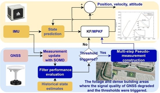
This study first conducts the performance evaluation of the KF in order to guarantee the unbiasedness of the historical state estimates used to construct pseudo-measurements. We use the SOMD method to estimate the noise covariance in the GNSS, $R_{GN}$. Meanwhile, we use another estimate of ${\overline{R}}_{GN}$ by calculating the correlation between the innovation and residual sequences. These two methods are different because the former is independent of the state estimate, while the latter is not. Further, we design the filter performance evaluation mechanism based on the difference between $R_{GN}$ and ${\overline{R}}_{GN}$. Then, a novel multi-step pseudo-measurement KF (MPKF) algorithm is proposed to enhance the precision of the state estimate.

The innovative points of this paper are summarized as below.

First, we use the SOMD method to evaluate the performance of the filter. On the one hand, $R_{GN}$ is estimated online to obtain a robust estimate for the filter; on the other hand, $R_{GN}$ is employed as a basic module for the filter evaluation to turn on or off the MPKF procedure by judging the unbiasedness of the historical estimates together with the calculation of the ${\overline{R}}_{GN}$ through the innovation and residual sequences.

Secondly, the MPKF algorithm is proposed, and the noise covariance of the MPKF is analyzed. Based on the performance evaluation, an adaptive mechanism is presented to suppress the negative effect led by the measurement noise. The multi-step pseudo-measurements are derived directly from the previous unbiased state estimates; therefore, if the actual measurement cannot maintain the desired accuracy, the multi-step pseudo-measurements can provide additional information to obtain a better estimated result for a given filter.

Finally, the MPKF algorithm is validated through a practical road test, demonstrating that it can enhance the accuracy of the navigation solution for the INS/GNSS integrated navigation system in comparison to other algorithms.

The remainder of this study is organized as follows. In the following section, the filter performance evaluation mechanism is proposed based on measurement noise covariance estimation (MNCE). In Section 3, the proposed MPKF algorithm is presented, meanwhile the analysis of uncertainties and the performance of the constructed multi-step pseudo-measurements are also discussed. The MPKF-based tightly-coupled INS/GNSS integrated algorithm is presented in Section 4. In Section 5, the real road experiment and its results are presented, and Section 6 draws the conclusions.

2. The MNCE and the Filter Performance Evaluation

By employing the SOMD, an MNCE is obtained, which is independent of the state estimate. By calculating the correlation between the innovation and residual sequences, another MNCE is obtained, which is relevant to the state estimate. Then, the filter performance evaluation mechanism is provided based on the difference between the two MNCEs.

2.1. The MNCE Based on the SOMD

Assuming that $z_k^{GN}$ and $z_k^{IN}$ are measurements of a signal $z_k^{True}$ from the GNSS and INS, the measurements are expressed by

$$\left\{\begin{array}{l}{z}_k^{GN}=z_k^{True}+{\epsilon }_k^{GN}+v_k^{GN}\\ z_k^{IN}=z_k^{True}+{\epsilon }_k^{IN}+v_k^{IN},\end{array}\right.$$

(1)

where ${\epsilon }_k^{GN}$ and ${\epsilon }_k^{IN}$ are the bias terms that can be assumed to be Gaussian random walk process [23], $k$ represents the $k\mathrm{th}$ epoch, and $v_k^{GN}$ and $v_k^{IN}$ are uncorrelated discrete noise:

$$\left\{\begin{array}{l}E[v_k^{GN}{\left(v_l^{GN}\right)}^T]=R_{GN}{\delta }_{k,l}\\ E[v_k^{IN}{\left(v_l^{IN}\right)}^T]=R_{IN}{\delta }_{k,l},\end{array}\right.$$

(2)

where ${\delta }_{k,l}$ is the Kronecker delta function.

The self-difference for each sensor is expressed by

$$\left\{\begin{array}{l}\Delta z_k^{GN}=z_k^{GN}-z_{k-1}^{GN}=\left[z_k^{True}-z_{k-1}^{True}\right]+\left[{\epsilon }_k^{GN}-{\epsilon }_{k-1}^{GN}\right]+\left[v_k^{GN}-v_{k-1}^{GN}\right]\\ \Delta z_k^{IN}=z_k^{IN}-z_{k-1}^{IN}=\left[z_k^{True}-z_{k-1}^{True}\right]+\left[{\epsilon }_k^{IN}-{\epsilon }_{k-1}^{IN}\right]+\left[v_k^{IN}-v_{k-1}^{IN}\right].\end{array}\right.$$

(3)

The mutual difference for the two sensors is expressed by

$$\begin{array}{l}\nabla z_k^{G-I}=\Delta z_k^{GN}-\Delta z_k^{IN}\\ =\left[{\epsilon }_k^{GN}-{\epsilon }_{k-1}^{GN}\right]-\left[{\epsilon }_k^{IN}-{\epsilon }_{k-1}^{IN}\right]+\left[v_k^{GN}-v_{k-1}^{GN}\right]-\left[v_k^{IN}-v_{k-1}^{IN}\right]\\ \approx \left[v_k^{GN}-v_{k-1}^{GN}\right]-\left[v_k^{IN}-v_{k-1}^{IN}\right],\end{array}$$

(4)

where the differences from the bias terms are neglected, because the numerical value of which is usually smaller than the noise terms. The noise covariance assumptions are expressed by

$$\left\{\begin{array}{l}E\left[v_k^{GN}{\left(v_k^{IN}\right)}^T\right]=0\\ E\left[v_k^{GN}{\left(v_{k-1}^{GN}\right)}^T\right]=0\\ E\left[v_k^{IN}{\left(v_{k-1}^{IN}\right)}^T\right]=0,\end{array}\right.$$

(5)

Then, $E\left[\nabla z_k^{G-I}{\left(\nabla z_k^{G-I}\right)}^T\right]$ is calculated by

$$\begin{array}{l}E\left[\nabla z_k^{G-I}{\left(\nabla z_k^{G-I}\right)}^T\right]\\ =E\left[v_k^{GN}{\left(v_k^{GN}\right)}^T\right]+E\left[v_{k-1}^{GN}{\left(v_{k-1}^{GN}\right)}^T\right]+E\left[v_k^{IN}{\left(v_k^{IN}\right)}^T\right]+E\left[v_{k-1}^{IN}{\left(v_{k-1}^{IN}\right)}^T\right].\end{array}$$

(6)

where $E\left[v_k^{IN}{\left(v_k^{IN}\right)}^T\right]$ and $E\left[v_{k-1}^{IN}{\left(v_{k-1}^{IN}\right)}^T\right]$ are neglected because the accuracy of the INS is much higher than that of the GNSS in the short term, i.e., $E\left[v_k^{IN}{\left(v_k^{IN}\right)}^T\right]\ll E\left[v_k^{GN}{\left(v_k^{GN}\right)}^T\right]$. Hence, the noise covariance of the GNSS $R_{GN}$ is expressed by

$$R_{GN}=\frac{E\left[v_k^{GN}{\left(v_k^{GN}\right)}^T\right]+E\left[v_{k-1}^{GN}{\left(v_{k-1}^{GN}\right)}^T\right]}{2}\approx \frac{E\left[\nabla z_k^{G-I}{\left(\nabla z_k^{G-I}\right)}^T\right]}{2}.$$

(7)

A sliding window method is employed to calculate $E\left[\nabla z_k^{G-I}{\left(\nabla z_k^{G-I}\right)}^T\right]$:

$$E\left[\nabla z_k^{G-I}{\left(\nabla z_k^{G-I}\right)}^T\right]=\frac{1}{W}{\displaystyle \sum _{l=0}^{W-1}\nabla z_{k-l}^{G-I}{\left(\nabla z_{k-l}^{G-I}\right)}^T},$$

(8)

where $W$ stands for the sliding window size.

The SOMD works well when the sequences $\nabla z_k^{G-I}$ are independent. However, due to the complex environments especially in urban areas, the independence in the mutual sequences might be violated. In this study, Burg’s method was used to calculate $R_{GN}$ if the independence was violated by the kernel density estimation (KDE) method [12].

The important advantages of the SOMD are summarized below:

(1)

$R_{GN}$ is only based on measurements and is independent of the state estimate error.

(2)

Given the measurements from the INS and GNSS, without any stated-related information, $R_{GN}$ can be estimated by the SOMD.

(3)

If there is a trend term bias in the noise, $R_{GN}$ is not affected because of the self-difference calculation.

So, we can use $R_{GN}$ as the reference, while another estimate that is not independent of the state estimate error can be obtained.

2.2. The MNCE Based on the Correlation between Innovation and Residual Sequences

For a general linear stochastic system, the process and observation models in the discrete-time form are expressed by

$$\left\{\begin{array}{l}{x}_k={\Phi }_{k,k-1}{x}_{k-1}+{\Gamma }_k{v}_k^P\\ z_k=H_k{x}_k+v_k^R,\end{array}\right.$$

(9)

where $x_k\in {ℝ}^n$ and $z_k\in {ℝ}^m$ represent the state vector and the measurement vector, respectively. $v_k^P$ and $v_k^R$ are the process noise and the measurement noise at the $k\mathrm{th}$ epoch, respectively, which are independent zero-mean white Gaussian vectors. ${\Gamma }_k$ stands for the noise-driven matrix. ${\Phi }_{k,k-1}$ and $H_k$ are the state transition matrix and observation matrix, respectively. The covariances of $v_k^P$ and $v_k^R$ are expressed by

$$\left\{\begin{array}{l}E[v_t^P{v}_{\tau }^P]=Q_k{\delta }_{t,\tau }\\ E[v_t^R{v}_{\tau }^R]=R_k{\delta }_{t,\tau }.\end{array}\right.$$

(10)

The state estimate ${\widehat{x}}_{k|k}$, the Kalman gain matrix $K_k$, and state error covariance $P_{k|k}$ are expressed by

$$\left\{\begin{array}{l}{K}_k=P_{k|k-1}{H}_k^T{\left[H_k{P}_{k|k-1}{H}_k^T+R_k\right]}^{-1}\\ {\widehat{x}}_{k|k}={\widehat{x}}_{k|k-1}+K_k\left[z_k-H_k{\widehat{x}}_{k|k-1}\right]\\ P_{k|k}=\left[I-K_k{H}_k\right]P_{k|k-1}.\end{array}\right.$$

(11)

The innovation is expressed by

$${\epsilon }_k\triangleq z_k-H_k{\widehat{x}}_{k|k-1},$$

(12)

where ${\widehat{x}}_{k|k-1}$ represents the one-step predicted state. The residual is expressed by

$${\eta }_k\triangleq z_k-H_k{\widehat{x}}_{k|k}.$$

(13)

The correlation of ${\epsilon }_k$ and ${\eta }_k$ is expressed by

$$\begin{array}{l}E\left[{\epsilon }_k{\eta }_k^T\right]=\\ H_{k}E\left[\left(x_k-{\widehat{x}}_{k|k-1}\right){\left(x_k-{\widehat{x}}_{k|k}\right)}^T\right]H_k^T+H_{k}E\left[\left(x_k-{\widehat{x}}_{k|k-1}\right){\left(v_k^R\right)}^T\right]+E\left[v_k^R{\left(x_k-{\widehat{x}}_{k|k}\right)}^T\right]H_k^T+R_k.\end{array}$$

(14)

Considering (11), the first term in the last line of (14) is calculated by:

$$H_{k}E\left[\left(x_k-{\widehat{x}}_{k|k-1}\right){\left(x_k-{\widehat{x}}_{k|k}\right)}^T\right]H_k^T=R_k{K}_k^T{H}_k^T,$$

(15)

The second one is $0$ because both $x_k$ and ${\widehat{x}}_{k|k-1}$ are independent of $v_k^R$. The third term is calculated by:

$$E\left[v_k^R{\left(x_k-{\widehat{x}}_{k|k}\right)}^T\right]H_k^T=-R_k{K}_k^T{H}_k^T.$$

(16)

By adding the four terms in (14), we can obtain $E\left[{\epsilon }_k{\eta }_k^T\right]=R_k$. Also, this is calculated by a sliding window method similar to (8).

It is worth noting that $R_k$ can be affected by the state estimate, because both ${\epsilon }_k$ and ${\eta }_k$ are state estimate-related terms, as shown in (12) and (13), respectively. Put differently, if the state estimate is unbiased, $R_k$ obtained by (14) can be seen as the ideal estimate. Otherwise, $R_k$ might be different from the ideal measurement noise covariance, because the first and the third term in (14) might not be the results calculated by (15) and (16).

2.3. The Filter Performance Evaluation

The SOMD method and the correlation between innovation and residual sequences were used to determine the filter performance in this study. The key idea is that the former is immune to the state estimate error, and the latter is relative with the state estimate error. Hence, the SOMD can provide a solid estimate of $R_{GN}$, which can be used as the reference compared to the other one.

For practical INS/GNSS applications, if the difference between $R_{GN}$ calculated using (7) and ${\overline{R}}_{GN}\left(=E\left[{\epsilon }_k{\eta }_k^T\right]\right)$ obtained by (14) is large, we can deduce that, during the calculation interval, the state estimates are biased; otherwise, the state estimates can be seen as unbiased.

3. Multi-Step Pseudo-Measurement for the KF

The accuracy of the KF relies on the precision of the measurement if the dynamic model behaves normally and the statistics of the process noise obey the a priori assumptions. To acquire more accurate measurements, one way is to utilize high-precision equipment directly, but at a higher cost as a result. Another way is to use several relatively low-precision sensors as an array simultaneously [24,25]. Inspired by the second methodology at the hardware level, we proposed the multi-step pseudo-measurement algorithm under the KF framework.

This paper used the difference between ${\overline{R}}_{GN}$ and $R_{GN}$ as the indicator for evaluating the filter performance of the KF. This is important for the proposed multi-step pseudo-measurement method, because the historical estimates employed to construct the multi-step pseudo-measurement should be unbiased, so that the uncertainty or noise of the multi-step pseudo-measurement can be seen as zero-mean term. Furthermore, the modified KF can obtain better accuracy estimates. Although the noises in multi-step pseudo-measurement are correlated in that the state estimates are correlated, they can be orthogonalized by a whitening method [26].

3.1. The Method of Constructing the Multi-Step Pseudo-Measurement

The derivation of the proposed multi-step pseudo-measurement is based on a linear system described by (9) and its corresponding assumptions. However, this method can be used in non-linear systems through appropriate modification. In Section 5, an EKF-based real road experiment is shown as a practical application for a non-linear application.

The multi-step pseudo-measurement is expressed by

$$\left\{\begin{array}{l}{z}_{k,k-2}^p=H_k^p{\Phi }_{k,k-2}{x}_{k-2}\\ z_{k,k-3}^p=H_k^p{\Phi }_{k,k-3}{x}_{k-3},\end{array}\right.$$

(17)

where $z_{k,k-i,}^{p}i=2, 3$ stands for the pseudo-measurement constructed from $x_{k-i}$, and $H_k^p$ is the pseudo-measurement matrix. Because the ideal state of $x_{k-i}$ cannot be obtained, it is replaced by ${\widehat{x}}_{k-i|k-i}+{\tilde{x}}_{k-i|k-i}$, and ${\tilde{x}}_{k-i|k-i}$ is the estimate error. Let ${\overline{v}}_{k,k-i}^p$ denote $H_k^p{\Phi }_{k,k-i}{\tilde{x}}_{k-i|k-i}$, the superscript $p$ here stands for ‘pseudo’; then, the augmented measurement equation can be rewritten in a compact form as ${\overline{z}}_k={\overline{H}}_k{\overline{x}}_k+{\overline{v}}_k$, whose terms are defined as

$$\left\{\begin{array}{l}{\overline{z}}_{\mathit{k}}\triangleq {\left[z_k,z_{k,k-2}^p,z_{k,k-3}^p\right]}^T\\ {\overline{H}}_k\triangleq {\left[H_k,H_k^p,H_k^p\right]}^T\\ {\overline{x}}_k\triangleq x_k\\ {\overline{v}}_k\triangleq diag{\left[v_k,{\overline{v}}_{k,k-2}^p,{\overline{v}}_{k,k-3}^p\right]}^T,\end{array}\right.$$

(18)

where $E\left[{\overline{v}}_{k,k-1}^p\right]=0$ when $E\left[{\tilde{x}}_{k-i|k-i}\right]=0$; again, this is why we proposed the filter performance evaluation method to judge the unbiasedness of the state estimates. Then, the variance of ${\overline{V}}_k$ is denoted as ${\overline{R}}_k$:

$${\overline{R}}_k\triangleq E\left[{\overline{V}}_k{\overline{V}}_k^T\right]=\left[\begin{array}{ccc}{R}_k& 0& 0\\ 0& R_{k-2}^P& {\left(R_{k-2,k-3}^P\right)}^T\\ 0& R_{k-2,k-3}^P& R_{k-3}^P\end{array}\right],$$

(19)

where the $0$ components are obtained based on the fact that $v_k$ is independent of ${\tilde{x}}_{k-2|k-2}$ and ${\tilde{x}}_{k-3|k-3}$. $R_{k-2}^P$ and $R_{k-2,k-3}^P={\left(R_{k-2,k-3}^P\right)}^T$ are expressed, respectively, by

$$R_{k-2}^P=H_k^p{\Phi }_{k,k-2}{\tilde{x}}_{k-2|k-2}{\tilde{x}}_{k-2|k-2}^T{\Phi }_{k,k-2}^T{\left(H_k^p\right)}^T=H_k^p{\Phi }_{k,k-2}{P}_{k-2|k-2}{\Phi }_{k,k-2}^T{\left(H_k^p\right)}^T,$$

(20)

$$\begin{array}{l}{R}_{k-2,k-3}^P=H_k^p{\Phi }_{k,k-2}{\tilde{x}}_{k-2|k-2}{\tilde{x}}_{k-3|k-3}^T{\Phi }_{k,k-3}^T{\left(H_k^p\right)}^T\\ \hspace{1em}\hspace{1em} =H_k^p{\Phi }_{k,k-2}{\Phi }_{k-2,k-3}{\tilde{x}}_{k-3|k-3}{\tilde{x}}_{k-3|k-3}^T{\Phi }_{k,k-3}^T{\left(H_k^p\right)}^T\\ \hspace{1em}\hspace{1em} =H_k^p{\Phi }_{k,k-3}{P}_{k-3|k-3}{\Phi }_{k,k-3}^T{\left(H_k^p\right)}^T,\end{array}$$

(21)

Moreover, (19) shows that ${\overline{R}}_k$ is not a diagonal matrix. To lighten the computational load on the inverse operation in calculating the Kalman gain, ${\overline{v}}_k$ can be transformed into independent measurements through the Cholesky decomposition [26]; then, ${\overline{R}}_k$ can be a diagonal matrix.

Then, the Kalman gain, the state estimate, and the error covariance are calculated, respectively, as

$${\overline{K}}_k=P_{k|k-1}{\overline{H}}_k^T{\left[{\overline{H}}_k{P}_{k|k-1}{\overline{H}}_k^T+{\overline{R}}_k\right]}^{-1},$$

(22)

$${\widehat{x}}_{k|k}={\Phi }_{k,k-1}{\widehat{x}}_{k-1|k-1}+{\overline{K}}_k\left[{\overline{z}}_{\mathbf{k}}-{\overline{H}}_k{\widehat{x}}_{k|k-1}\right],$$

(23)

$${\overline{P}}_{k|k}=\left[I-{\overline{K}}_k{\overline{H}}_k\right]P_{k|k-1}.$$

(24)

It can be noticed that the optimal filter requires that the noise of the measurement should be orthogonal to the state estimate error ${\tilde{x}}_{k|k-1}$; otherwise, the Kalman gain cannot be calculated by (22). In this study, the noise of the constructed multi-step pseudo-measurement is not orthogonal to ${\tilde{x}}_{k|k-1}$; however, we used (22) to calculate the Kalman gain because this approximation can achieve an acceptable navigation solution accuracy.

In this paper, we only used $i=2, 3$ to construct the pseudo-measurements because, if $i=1$, there is a linear correlation between the one-step pseudo-observation and the state prediction, and if $i>3$, more computational loads are needed and more process uncertainties might be introduced.

Based on the proposed filter performance evaluation method, we designed the following mechanism to utilize the multi-step pseudo-measurements, which were constructed using the historical unbiased state estimates.

If $R_{GN}$ is greater than its nominal value (e.g., from the GNSS receiver manual), and there is no vast difference between $R_{GN}$ and ${\overline{R}}_{GN}$, the current filter performance can be considered normal, i.e., the estimates are unbiased and can be employed for the construction. Then, a multi-step pseudo-observation procedure is initiated to suppress the errors caused by deteriorating measurement systems. For INS/GNSS applications, the majority of navigation solution errors come from this circumstance. So, this is the key problem that this paper aimed to tackle.

If $R_{GN}$ decreases to the normal level, it indicates that the accuracy of the measurement system is acceptable, and the pseudo-observation mechanism is exited to return to the normal filtering procedure. On the one hand, even if $R_{GN}$ is unchanged, the proposed multi-step pseudo-observation algorithm still has the ability to enhance the accuracy of the navigation solution, only if the historical estimates are unbiased. This is left for our future work. On the other hand, if the filter performance degrades due to other disturbances, such as model errors or changes in process noises but $R_{GN}$, some other adaptive algorithms can be employed to improve the navigation solutions.

3.2. The Analysis of the Performance of the Proposed MPKF

The matrix $P_{k|k}$ can be used as the metric to evaluate the performance of a given filter [27]. Compared to the KF, (24) can generate a smaller ${\overline{P}}_{k|k}$ than $P_{k|k}$.

The derivation details are as follows. Through the Cholesky decomposition, ${\overline{R}}_k^p$ is expressed by

$${\overline{R}}_k^p\triangleq \left[\begin{array}{cc}{R}_{k-2}^P& R_{k-2,k-3}^P\\ R_{k-2,k-3}^P& R_{k-3}^P\end{array}\right]=L_k{L}_k^T.$$

(25)

Then, ${\overline{L}}_k$ is defined as

$${\overline{L}}_k=\left[\begin{array}{cc}I& 0\\ 0& L_k\end{array}\right],$$

(26)

where $I$ is the identity matrix of the corresponding dimension. By left multiplying ${\overline{L}}_k^{-1}$, the noise term in (18) is expressed by

$${\overline{v}}_k^{*}={\overline{L}}_k^{-1}{\overline{v}}_k,$$

(27)

Then, the covariance of ${\overline{R}}_k^{*}$ is expressed by

$${\overline{R}}_k^{*}=E\left[{\overline{v}}_k^{*}{\left({\overline{v}}_k^{*}\right)}^T\right]={\overline{L}}_k^{-1}\left[\begin{array}{cc}{R}_k& 0\\ 0& {\overline{R}}_k^p\end{array}\right]{\left({\overline{L}}_k^{-1}\right)}^T=\left[\begin{array}{cc}{R}_k& 0\\ 0& I\end{array}\right].$$

(28)

Now, all the noise terms are independent, and ${\overline{P}}_{k|k}$ can be calculated through the sequential Kalman filtering process as follows:

$$\left\{\begin{array}{l}{\left[K_k\right]}^0=P_{k|k-1}{H}_k^T{\left[H_k{P}_{k|k-1}{H}_k^T+R_k\right]}^{-1}\\ {\left[{\widehat{x}}_{k|k}\right]}^0={\Phi }_{k,k-1}{\widehat{x}}_{k-1|k-1}+K_k\left[z_k-H_k{\widehat{x}}_{k|k-1}\right]\\ {\left[P_{k|k}\right]}^0=\left[I-{\left[K_k\right]}^0{H}_k\right]P_{k|k-1},\end{array}\right.$$

(29)

where ${\left[K_k\right]}^0$, ${\left[{\widehat{x}}_{k|k}\right]}^0$, and ${\left[P_{k|k}\right]}^0=P_{k|k}$ are the estimation results of the standard KF. Then, the pseudo-observation is employed to calculate ${\overline{P}}_{k|k}$:

$$\left\{\begin{array}{l}{\overline{K}}_k={\left[P_{k|k}\right]}^0{\left({\overline{H}}_k^{*}\right)}^T{\left[{\overline{H}}_k^{*}{\left[P_{k|k}\right]}^0{\left({\overline{H}}_k^{*}\right)}^T+I\right]}^{-1}\\ {\widehat{x}}_{k|k}={\left[{\widehat{x}}_{k|k}\right]}^0+{\overline{K}}_k\left[{\overline{z}}_k^{*}-{\overline{H}}_k^{*}{\left[{\widehat{x}}_{k|k}\right]}^0\right]\\ {\overline{P}}_{k|k}=\left[I-{\overline{K}}_k{\overline{H}}_k^{*}\right]{\left[P_{k|k}\right]}^0.\end{array}\right.$$

(30)

where

$${\left\{\begin{array}{l}{\overline{z}}_k^{*}=L_k^{-1}\left[z_{k,k-2}^p,z_{k,k-3}^p\right]\\ {\overline{H}}_k^{*}=L_k^{-1}{\left[H_k^p,H_k^p\right]}^T.\end{array}\right.}^T$$

(31)

It can be concluded that ${\overline{P}}_{k|k}<P_{k|k}$, in that ${\overline{K}}_k{\overline{H}}_k^{*}$, is a positive definite diagonal matrix. This conclusion can also be illustrated by an intuitive way in that a more reliable measurement can result in a greater Kalman gain.

However, if the noise of the multi-step pseudo-observation is greater than a threshold, it has a negative impact on the state estimation; so, it is necessary to set a threshold for employing the pseudo-observation method. Because the ideal state $x_k$ could not be obtained, given $z_k$ and ${\widehat{x}}_{k|k}$, the residual ${\eta }_k$ can be obtained. ${\widehat{x}}_{k|k}$ can be seen as the optimal estimate from the standard KF procedure; meanwhile, the pseudo-observation-based innovation ${\epsilon }_k^p$ is expressed by

$$\left\{\begin{array}{l}{\eta }_k=z_k-H_k{\widehat{x}}_{k|k}\\ {\epsilon }_k^p\triangleq {\left[z_{k,k-2}^p,z_{k,k-3}^p\right]}^T-{\left[H_k^p,H_k^p\right]}^T{\widehat{x}}_{k|k-1}.\end{array}\right.$$

(32)

The 2-norm of ${\eta }_k$ and ${\epsilon }_k^p$ can be used as the filter performance index to decide whether the pseudo-observation procedure executes or not. If the following inequation holds, the pseudo-observation procedure executes.

$$\frac{1}{2}{‖{\epsilon }_k^p{\left({\epsilon }_k^p\right)}^T‖}_2\le {‖{\eta }_k{\eta }_k^T‖}_2.$$

(33)

Remark 1.

For a specific application, not all state variables are equally crucial. Therefore, (33) can be adapted to focus on the relevant state variables. Additionally, it is important to note that, if some state variables differ by an order of magnitude in value, the variable with the larger numerical value has a greater impact on the equation’s norm. For INS/GNSS applications, the numerical value of the position, velocity, and attitude are greater than other elements, such as the bias of the gyroscope drift and the accelerometer error.

Remark 2.

For applications in which no actual redundancy measurement exists, (33) must be used.

Remark 3.

In the above derivation, $H_k^p=H_k$. For different applications, the selection of $H_k^p$ can be designed according to the practical engineering circumstance. Meanwhile, the scalar $\frac{1}{2}$ can also be tuned for a certain application.

4. The MPKF-Based Tightly INS/GNSS Integration Algorithm

The loosely coupled (LC) and tightly coupled (TC) integration methods are usually employed in INS/GNSS applications. Compared to the LC algorithm, the TC algorithm could obtain a better navigation solution accuracy as it incorporates the difference in pseudo-range and pseudo-range rate between the INS and GNSS in the measurement function. We adopted the EKF as the information fusion algorithm; meanwhile, the error model of the INS was used for the state prediction function and the measurement function.

4.1. The System Function and the Measurement Function

The details of the mechanism for INS can be found in many references, so, they were omitted in this paper. In short, the system model is expressed as in (9). The state vector is expressed by:

$$x={\left[{\phi }^n,\delta {\mathit{V}}^n,\delta L,\delta \lambda ,\delta h,{\epsilon }^b,{\nabla }^b,\delta t_u,\delta t_{ru}\right]}^T\in {ℝ}^{17},$$

(34)

where ${\phi }^n\in {ℝ}^3$ stands for the attitude error; $\delta {\mathit{V}}^n\in {ℝ}^3$ represents the velocity error; and $\delta L, \delta \lambda , \delta h$ represent the error in latitude, longitude, and height, respectively. ${\epsilon }^b\in {ℝ}^3$ and ${\nabla }^b\in {ℝ}^3$ stand for the gyroscope drift and the accelerometer error, respectively. $\delta t_u$ and $\delta t_{ru}$ are the GNSS receiver’s clock offset and its drift, respectively. The superscript $n$ and $b$ represent the navigation frame and the body frame, respectively. The transition functions of the relative state are expressed by (35)–(40):

$${\dot{\phi }}^n=-\left({\omega }_{ie}^n+{\omega }_{en}^n\right)\times {\phi }^n+\left(\delta {\omega }_{ie}^n+\delta {\omega }_{en}^n\right)-C_b^n{\epsilon }^b,$$

(35)

where the subscript $e$ stands for the earth-centered, earth-fixed frame; ${\omega }_{ie}^n$ is the earth rate; and ${\omega }_{en}^n$ is the rate of the $n$-frame with respect to the $e$-frame. The direction cosine matrix $C_b^n$ represents the transition from the $b$-frame to the $n$-frame. The navigation frame is the local-level frame with axes pointing to east ($x$), north ($y$), and up ($z$) directions.

$$\left[\begin{array}{c}\delta \dot{L}\\ \delta \dot{\lambda }\\ \delta \dot{h}\end{array}\right]=\left[\begin{array}{c}\frac{\delta V_y^n}{R_M+h}-\frac{V_y^n}{{\left(R_M+h\right)}^2}\delta h\\ \frac{\delta V_x^n}{\left(R_N+h\right)\cos L}-\frac{V_x^n}{{\left(R_N+h\right)}^2\cos L}\delta h+\frac{V_x^n\cdot \tan L}{\left(R_N+h\right)\cos L}\delta L\\ V_z^n\end{array}\right],$$

(36)

where $V_x^n$, $V_y^n$, and $V_z^n$ are the velocity errors in the corresponding directions. The meridian and transverse radius of curvature are denoted by $R_M$ and $R_N$, respectively.

$$\delta {\dot{\mathit{V}}}^n=-f^n\times f^n+\delta {\mathit{V}}^n\times \left(2{\omega }_{ie}^n+{\mathit{\omega }}_{en}^n\right)+V^n\times \left(2\delta {\mathit{\omega }}_{ie}^n+\delta {\mathit{\omega }}_{en}^n\right)+\delta g^n+C_b^n{\nabla }^b,$$

(37)

where $f^n$ denotes the specific force error and $\delta g^n$ is the gravitational error.

The error modes for the gyroscopes, the accelerometers, and the clock offset are assumed as first-order Markov processes (FOGM):

$$\left\{\begin{array}{l}\epsilon ={\epsilon }^b+{\epsilon }^r\\ {\dot{\epsilon }}^b=0\\ {\dot{\epsilon }}^r=-\frac{1}{C_{tg}}{\epsilon }^r+{\omega }_g,\end{array}\right.$$

(38)

$${\dot{\nabla }}^b=-\frac{1}{C_{ta}}{\nabla }^b+{\omega }_a,$$

(39)

$$\begin{array}{l}\delta {\dot{t}}_u=\delta t_{ru}+{\omega }_u\\ \delta {\dot{t}}_{ru}=-\beta \delta t_{ru}+{\omega }_{ru},\end{array}$$

(40)

where ${\epsilon }^b$ is the gyroscope bias, ${\epsilon }^r$ represents the FOGM, and ${\omega }_g$ represents the noise. $C_{tg}$ and $C_{ta}$ denote the coefficients of the correlation time for the gyroscopes and accelerometers, respectively. ${\omega }_g$, ${\omega }_a$, ${\omega }_u$, and ${\omega }_{ru}$ are Gaussian white noises.

The observation model is expressed by:

$$\left\{\begin{array}{l}\delta {\rho }_j={\rho }_{IN}^j-{\rho }_{GN}^j\hfill \\ \delta {\dot{\rho }}_j={\dot{\rho }}_{IN}^j-{\dot{\rho }}_{GN}^j,\hfill \end{array}\right.$$

(41)

where

$$\begin{array}{l}\left\{\begin{array}{l}{\rho }_{IN}^j=\sqrt{{(x_{IN}-x_{sat}^j)}^2+{(y_{IN}-y_{sat}^j)}^2+{(z_{IN}-z_{sat}^j)}^2}\hspace{1em}\\ {\dot{\rho }}_{IN}^j=\frac{x_{IN}-x_{sat}^j}{{\rho }_{IN}^j}\frac{\partial x_{IN}}{\partial t}+\frac{y_{IN}-y_{sat}^j}{{\rho }_{IN}^j}\frac{\partial y_{IN}}{\partial t}+\frac{z_{IN}-z_{sat}^j}{{\rho }_{IN}^j}\frac{\partial z_{IN}}{\partial t}\hspace{1em}\end{array}\right.\\ \left\{\begin{array}{l}{r}^j=\sqrt{{(x-x_{sat}^j)}^2+{(y-y_{sat}^j)}^2+{(z-z_{sat}^j)}^2}\\ {\dot{r}}^j=\frac{x-x_{sat}^j}{r^j}\frac{\partial x}{\partial t}+\frac{y-y_{sat}^j}{r^j}\frac{\partial y}{\partial t}+\frac{z-z_{sat}^j}{r^j}\frac{\partial z}{\partial t}\\ {\rho }_{GN}^j=r^j+c\left(\delta t_u-\delta T^j\right)+{\Delta }_{ion}+{\Delta }_{trop}+v_{\rho }^j\\ {\dot{\rho }}_{GN}^j={\dot{r}}^j+c\left(\delta {\dot{t}}_u-\delta {\dot{T}}^j\right)+v_{\dot{\rho }}^j,\end{array}\right.\end{array}$$

(42)

where $[x_{IN},y_{IN},z_{IN}]$ and $[x,y,z]$ represent the coordinate of the INS and the true position in the $e$-frame, respectively. The position of the $j\mathrm{th}$ satellite is denoted by $[x_{sat}^j,y_{sat}^j,z_{sat}^j]$. $c$ is the light speed. ${\Delta }_{ion}$ and ${\Delta }_{trop}$ are propagation delays of the ionosphere and troposphere, respectively. $v_{\rho }^j$ and $v_{\dot{\rho }}^j$ are the measurement noises. Usually, ${\Delta }_{ion}$ and ${\Delta }_{trop}$ can be calculated through the Klobuchar model and the troposphere delay model, respectively [28].

To sum up, the model represented in an EKF frame is expressed by:

$$\left\{\begin{array}{l}{x}_k=A_{k,k-1}{x}_{k-1}+{\Gamma }_k{v}_k^P\\ z_k={{\rm B}}_k{x}_k+v_k^R,\end{array}\right.$$

(43)

where $A_{k,k-1}$, ${\Gamma }_k$, and $v_k^P$ are obtained using (35)–(40); $z=\left[\delta {\rho }_j,\delta {\dot{\rho }}_j\right]$; ${\mathbf{B}}_k=\partial \mathbf{\Xi }/\partial {\widehat{x}}_{k/k-1}$; and $\Xi$ is calculated using (41) and (42).

The standard EKF evolves as follows [29]:

$$\left\{\begin{array}{l}{\widehat{x}}_{k|k-1}=A_{k,k-1}{\widehat{x}}_{k-1|k-1}\hfill \\ P_{k|k-1}=A_{k,k-1}{P}_{k-1|k-1}{A}_{k,k-1}^T+{\Gamma }_k{Q}_{k-1}{\Gamma }_k^T,\hfill \end{array}\right.$$

(44)

$$\left\{\begin{array}{l}{K}_k=P_{k|k-1}{{\rm B}}_k^T{\left({{\rm B}}_k{P}_{k|k-1}{{\rm B}}_k^T+R_k\right)}^{-1}\\ {\widehat{x}}_{k|k}={\widehat{x}}_{k|k-1}+K_k\left(z_k-{{\rm B}}_k{\widehat{x}}_{k|k-1}\right)\\ P_{k|k}=\left(I-K_k{{\rm B}}_k\right)P_{k|k-1}.\end{array}\right.$$

(45)

4.2. The Proposed MPKF-Based Algorithm for the TC INS/GNSS Integration System

The main idea of the MPKF is illustrated in Figure 1.

All the blocks proposed in this paper are colored blue. The upper part stands for the regular EKF procedure. The lower part is our proposed architecture for enhancing the precision of the navigation solution. By employing the SOMD, which is colored green, we can obtain $R_{GN}$. On the one hand, $R_{GN}$ is fed to the measurement update portion for achieving a robust filter; on the other hand, the use of a multi-step pseudo-observation construction depends on the trend of $R_{GN}$ and the filter performance evaluation mechanism.

For GNSS/INS TC integration, although the 17-dimesion vector is used as the state, the position, velocity, and attitude are considered for most applications. Hence, only these nine variables were taken into consideration for MP. So, $H_k^p$ is expressed by

$$H_k^p=\left[\begin{array}{cccc}{I}_{3\times 3}& 0& 0& 0\\ 0& I_{3\times 3}& 0& 0\\ 0& 0& I_{3\times 3}& 0\\ 0& 0& 0& 0_{8\times 8}\end{array}\right],$$

(46)

$H_k^p$ is not the same as the matrix $H_k$ in the measurement equation for GNSS/INS TC integration.

The pseudocode of the MPKF-based INS/GNSS is summarized in Algorithm 1.

Algorithm 1. The pseudocode of the MPKF-based INS/GNSS application

Input: ${\widehat{x}}_0, P_0, Q_0, R_k=diag\left(R_{GN}\right)$. Prediction: 1. Calculate ${\widehat{x}}_{k|k-1}$ and $P_{k|k-1}$ via (44). Observation update (switch between the regular KF or MPKF): 1. Calculate the $\nabla z_k^{G-I}$ via (3) and (4). 2. Gaussian distribution of $\nabla z_k^{G-I}$ test via the KDE method [30]: 3. if $\nabla z_k^{G-I}\sim Gaussian$ Calculate $R_{GN}$ via (7) and (8). else $R_{GN}=\mathrm{Burg}’\mathrm{s} \mathrm{Algorithm}(\nabla z_k^{G-I})$. end $R_k=diag\left(R_{GN}\right)$. 4. if $R_{GN}$ exceeds the normal level (via filter performance evaluation) MPKF procedure via (22)–(24). else Regular KF procedure via (45). end Outputs: ${\widehat{x}}_{k|k}$, $P_{k/k}$.

5. Experiment

To verify the proposed method, we used the data obtained in a field experiment in Tianjin City, China. The INS was IMU-ISA-100C, which is a product from the NovAtel Company, and the GNSS was a differential receiver. After post-processing by the NovAtel Inertial Explorer, the ground truth can be obtained, and 1 cm and 2 cm are the horizontal accuracy and vertical accuracy. The key performance parameters of the devices are shown in

Table 1. Performance parameters of the IMU-ISA-100C gyroscopes.

Gyroscope Parameters
Raw data rate	200 Hz
Bias stability (In-run)	≤0.05 deg/h
Full-scale measurement range	±495 deg/s
Angular random walk	0.012 deg/√h
Scale factor non-linearity	≤100 ppm

,

Table 2. Performance parameters of the IMU-ISA-100C accelerometers.

Accelerometer Parameters
Raw data rate	200 Hz
Bias stability (In-run)	≤100 μg
Full-scale measurement range	±10 g
Velocity random walk	≤100 μg/√Hz
Scale factor non-linearity	≤100 ppm

and

Table 3. Performance parameters of the IMU-ISA-100C GNSS receiver.

Horizontal Position Accuracy of GNSS (RMS)
Single-point L1/L2	1.20 m
SBAS	0.60 m
DGPS	0.40 m

.

5.1. Experiment Initialization

The elements in process noise covariance $Q_0$ for INS were obtained through offline calibration when the vehicle was in a stationary state. The elements for the GNSS were set according to the specifications. For $R_0$, we adopted $1.2$ for the pseudo-range and $0.12$ for the pseudo-range rate according to the manual:

$$\begin{array}{l}\sqrt{Q_0}=diag[std(gy{o}_x),std(gy{o}_y),std(gy{o}_y),std(ac{c}_x),std(ac{c}_y),std(ac{c}_z),1\times {10}^{-4},1\times {10}^{-5}]\\ R_0=diag[1.2,1.2,1.2,1.2,0.12,0.12,0.12,0.12],\end{array}$$

(47)

where $std(gy{o}_x)$ denotes the standard deviation of the x-axis gyroscope during the stationary interval.

The bias terms of INS were set as follows:

$$\begin{array}{l}{\epsilon }_{gx}={\epsilon }_{gy}={\epsilon }_{gz}=-5.810940718937726\times {10}^{-8}(\mathrm{rad}/\mathrm{s})\\ {{\epsilon }^b}_0=[{\epsilon }_{gx},{\epsilon }_{gx},{\epsilon }_{gx}],\end{array}$$

(48)

$$\begin{array}{l}{\nabla }_{ax}={\nabla }_{ay}={\nabla }_{az}=-0.054495220989616\left(\mathrm{mg}\right)\\ {{\nabla }^b}_0=[{\nabla }_{ax},{\nabla }_{ay},{\nabla }_{az}],\end{array}$$

(49)

The initial ${\widehat{x}}_0$ and ${\widehat{P}}_0$ were set, respectively, as follows:

$${\widehat{x}}_0={\left[0^3,0^3,0^3,{{\epsilon }^b}_0,{{\nabla }^b}_0,1.0,0.1\right]}^T,$$

(50)

$${\widehat{P}}_0=diag\left[{\widehat{x}}_0{\left({\widehat{x}}_0\right)}^T\right],$$

(51)

where ${\widehat{P}}_0$ is calculated through (51) because, in this study, the state error model was adopted.

We employed the standard extended KF (SKF), EIAKF [31], MCEKF [32], ERMAKF [28], and our proposed MPKF for comparative analysis. Among them, MCEKF is the improved EKF algorithm based on the maximum correntropy criterion. The root-mean-square error (RMSE) was adopted for estimate error comparisons. As an example, the 3-dimensional position error is expressed by:

$$RMS{E}_{postion}=\sqrt{\frac{1}{M}{\displaystyle \sum _{i=1}^M\left[{\left({\widehat{L}}_i^{meter}-L_i^{meter}\right)}^2+{\left({\widehat{\lambda }}_i^{meter}-{\lambda }_i^{meter}\right)}^2+{\left({\widehat{h}}_i-h_i\right)}^2\right]}},$$

(52)

where $\left[{\widehat{L}}_i^{meter},{\widehat{\lambda }}_i^{meter},{\widehat{h}}_i\right]$ and $\left[L_i^{meter},{\lambda }_i^{meter},h_i\right]$ are the $i\mathrm{th}$ epoch estimate and ground truth in latitude, longitude, and height, respectively, with units in meters; and $M$ is the total epochs.

Figure 2 shows the trajectory of the vehicle, with the silver-color-blocked area representing the dense foliage area and the yellow-blocked one indicating the dense building area. In these two areas, the GNSS signal quality deteriorates, as indicated by the red color, the white trajectory represents the SKF resolution The yellow trajectory represents the ground truth. Figure 3 and Figure 4 show the GNSS-alone errors in positioning for the two blocks. We can see that, in the two areas, the positioning errors grow rapidly. In the eastward and northward directions, the maximum values exceed 40 m.

5.2. Experimental Results

5.2.1. Navigation Solution Error Comparisons in the Foliage Environment

First, we present Figure 5 for illustrating the flag that indicates if the pseudo-measurements were used.

The threshold values for the pseudo-range and pseudo-range rate were set, respectively, to:

$$\left\{\begin{array}{l}treshol{d}_{pseudo range}=2\ast R_{pseudo range}^{\mathrm{nominal}}=2.4 \mathrm{m}\\ treshol{d}_{pseudo range-rage}=4\ast R_{pseudo range-rate}^{\mathrm{nominal}}=0.48 \mathrm{m}/\mathrm{s}.\end{array}\right.$$

(53)

The threshold should be modified for different applications when different sensors are used. It can be seen from this figure that, if both the values estimated of the pseudo-range and pseudo-range rate estimated by SOMD exceed their respective thresholds, the MPKF is employed. The first overlap interval corresponds to the densely wooded area in the actual trajectory, while the second overlap interval corresponds to the area with dense buildings. The triggering conditions are consistent with the experiment environments.

Figure 6 illustrates the position, velocity, and attitude errors of these algorithms in the 80–120 s interval of the navigation solution. It can be observed that the proposed algorithm achieves favorable results across statistical measures, such as the median, mean, and quartiles. The positioning error of the MPKF is reduced by about 20% and 32% compared to the ERMAKF and SKF (5.08 m vs. 6.39 m and 7.47 m), respectively. The velocity error of the MPKF is improved by 10% and 47% compared to ERMAKF and MCEKF (0.30 m/s vs. 0.33 m/s and 0.57 m/s), respectively. For the attitude error, the improvement is of about 58% and 38% compared to the ERMAKF and MCEKF (0.18° vs. 0.43° and 0.29°), respectively.

For further analysis, Figure 7, Figure 8 and Figure 9 present the results of each component of the navigation solution.

The interval with the largest errors is between 40 s and 120 s. During this period, the GNSS signal quality sharply declines, and due to the limited robustness of the EKF and EIAKF against the outliers, the errors of these two algorithms are the highest. This is reflected in the positioning errors, where the maximum longitude error approaches 20 m, while for latitude, it is 5 m. In terms of the velocity errors, the maximum error in the eastward velocity is close to 2 m per second, and the northward error exceeds 1 m. The performance of the MCEKF surpasses that of the EKF and EIAKF, as this algorithm considers the non-Gaussian distribution of noise and is based on the MCC rather than the MSE criterion. The ERMAKF and MPKF based on the SOMD exhibit the best performance, as these two algorithms provide estimates of the GNSS noise variance. Furthermore, the MPKF, when detecting a deterioration in the GNSS signal quality, effectively suppresses the impact of the actual measurement system’s accuracy degradation by using multi-step pseudo-observations.

For simplicity, please refer to [28] for the detailed change in $R_{GN}$.

The RMSEs during 80–120 s for different algorithms are shown in

Table 4. RMSEs during 80–120 s (the foliage area).

Algorithm	Longitude (m)	Latitude (m)	Height (m)	East Velocity (m/s)	North Velocity (m/s)	Up Velocity (m/s)	Pitch (°)	Roll (°)	Yaw (°)
SKF	5.4947	1.2624	5.6873	0.6415	0.2246	0.2221	0.2785	0.2165	0.0485
EIAKF	6.4426	1.8995	4.5234	0.6779	0.3255	0.1585	0.2784	0.2645	0.0454
ERMAKF	5.0849	1.9429	4.1101	0.2884	0.2544	0.1006	0.2783	0.3518	0.0312
MCEKF	5.1312	1.1843	5.3578	0.6001	0.2009	0.2183	0.2616	0.2031	0.0483
MPKF	3.6748	1.401	3.338	0.2260	0.1821	0.1726	0.1531	0.1234	0.0502

.

5.2.2. Navigation Solution Error Comparisons in the Dense Building Area Environment

From Figure 10, it can be concluded that, in dense urban environments, the MPKF shows significant improvements in estimating the accuracy compared to the other algorithms. In terms of positioning, the accuracy is improved by 34% and 42% compared to the ERMAKF and MCEKF, respectively. In terms of speed, the improvements are 35% and 49% compared to the ERMAKF and MCEKF, respectively. For the attitude error, the improvements are 48% and 38% compared to the ERMAKF and MCEKF, respectively.

Figure 11, Figure 12 and Figure 13 show the estimate results of each component in the algorithms. The signal quality of the GNSS deteriorates significantly between 260 s and 300 s, resulting in the poorest performance in positioning estimate for the EKF and IEAKF. Although the IEAKF estimates the noise covariance of the GNSS, the algorithm’s robustness deteriorates due to the large errors in the state estimate results in this interval. It is worth noting that, in the estimate results of the MPKF, the latitude estimate and eastward velocity results are slightly inferior to those of the ERMAKF, mainly because the positive effect brought by pseudo-range observations weakens. Therefore, one of the future research directions is how to switch between the conventional EKF and MPKF more quickly.

The RMSEs during 260–300 s for different algorithms are shown in

Table 5. RMSEs during 260–300 s (the dense building area).

Algorithm	Longitude (m)	Latitude (m)	Height (m)	East Velocity (m/s)	North Velocity (m/s)	Up Velocity (m/s)	Pitch (°)	Roll (°)	Yaw (°)
SKF	4.3375	1.1487	3.6983	0.3777	0.1371	0.1732	0.2027	0.07	0.0887
EIAKF	3.9725	3.3917	3.4764	0.2469	0.1951	0.1184	0.2186	0.0932	0.1281
ERMAKF	3.493	1.2287	2.8754	0.2743	0.1631	0.1085	0.1497	0.2148	0.038
MCEKF	3.9398	1.0825	3.2441	0.3459	0.1304	0.1618	0.1906	0.065	0.0922
MPKF	3.3464	3.1183	3.0192	0.2154	0.3022	0.1697	0.0619	0.0863	0.1032

.

5.3. Discussion

During the initial phase of the degraded GNSS signal quality, the MPKF method demonstrates a superior accuracy in estimating the position, velocity, and attitude compared to the alternative algorithms. This is partly due to the estimate of noise covariance in the GNSS signal and partly due to the smaller uncertainty of the state transition matrix in this interval. In the second section, the MPKF also achieved a high estimate accuracy, but did not perform as well in latitude and eastward velocity estimates as in the first section. This is mainly due to the more pronounced multi-path effects in dense road sections, and the presence of severe heavy-tailed noise variance distribution. As shown in Figure 11, the error increased from 280 s to 300 s and might be worse if the time was longer. Therefore, future work will also include more testing with different GNSS-challenging areas and also lower grade GNSS and IMU systems.

With the permissions of the authors in Ref. [28], we used the same $Q_0$, $R_0$, and IMU bias parameters. Usually, for the GNSS clock bias and drift, especially, for the clock bias, a larger $Q=10$ or $Q=100$ should be used. Meanwhile, for TC integration applications, sufficient attention should be paid when using the standard deviation values from the GNSS receiver for $R_0$ because they are provided in the position domain, not the measurement domain. Additionally, although the reference position has an accuracy of centimeters, i.e., accurate to the second decimal place, we used four decimal places to avoid introducing rounding errors and truncation errors during the calculation process.

This paper focused on the application of the proposed MPKF algorithm in TC integrated navigation. For the LC mechanisms, the algorithm is also applicable, requiring only corresponding changes in the state transition matrix and measurement matrix.

Furthermore, in the current field of autonomous driving, the use of LiDAR and cameras is becoming increasingly widespread and mature. The noise of these sensors also varies with different environments. Therefore, the SOMD-based multi-step pseudo-measurement approach proposed in this paper is also applicable to the fusion of more sensor information. Future work will also consider the combination of multi-sensor elastic fusion and multi-step pseudo-measurements.

6. Conclusions

This paper proposes a multi-step pseudo-observation algorithm based on filter performance evaluation. (1) According to the outcomes of performance evaluation based on the SOMD, it can be determined whether the actual measurement system is in a degraded state. (2) When the actual measurement system noise increases, unbiased historical state estimates are used to construct pseudo-observations. Benefiting from the good short-term self-sustainability of the INS, and compared to simply expanding the noise covariance matrix, the proposed algorithm makes more full use of historical filtering information, thereby improving the estimate accuracy. (3) Actual vehicle tests verified that, in urban navigation applications, especially in complex environments, the proposed algorithm shows significant improvements compared to adaptive algorithms based on the MSE criterion and MCEKF algorithms based on the MCC criterion.

References

1. Grewal, M.S.; Weill, L.R.; Andrews, A.P. Global Positioning Systems, Inertial Navigation, and Integration; John Wiley: Hoboken, NJ, USA, 2001; pp. 9–10. [Google Scholar]
2. Zhu, N.; Marais, J.; Betaille, D.; Berbineau, M. GNSS Position Integrity in Urban Environments: A Review of Literature. IEEE Trans. Intell. Transp. Syst. 2018, 19, 2762–2778. [Google Scholar] [CrossRef]
3. Kim, Y.; An, J.; Lee, J. Robust Navigational System for a Transporter Using GPS/INS Fusion. IEEE Trans. Ind. Electron. 2018, 65, 3346–3354. [Google Scholar] [CrossRef]
4. Xu, H.; Hsu, L.-T.; Lu, D.; Cai, B. Sky visibility estimation based on GNSS satellite visibility: An approach of GNSS-based context awareness. GPS Solut. 2020, 24, 59. [Google Scholar] [CrossRef]
5. Godha, S.; Cannon, M.E. GPS/MEMS INS integrated system for navigation in urban areas. GPS Solut. 2007, 11, 193–203. [Google Scholar] [CrossRef]
6. Xiang, Z.; Zhang, T.; Wang, Q.; Jin, S.; Nie, X.; Duan, C.; Zhou, J. A SINS/GNSS/2D-LDV integrated navigation scheme for unmanned ground vehicles. Meas. Sci. Technol. 2023, 34, 125116. [Google Scholar] [CrossRef]
7. Guo, J.; Wang, C.; Chen, G.; Xu, X.; Zhao, Q. BDS-3 precise orbit and clock solution at Wuhan University: Status and improvement. J. Geod. 2023, 97, 15. [Google Scholar] [CrossRef]
8. Groves, P.D. Principles of GNSS, Inertial, and Multisensor Integrated Navigation Systems; Artech House: London, UK, 2008; pp. 363–387. [Google Scholar]
9. Sun, R.; Zhang, Z.; Cheng, Q.; Ochieng, W.Y. Pseudorange error prediction for adaptive tightly coupled GNSS/IMU navigation in urban areas. GPS Solut. 2021, 26, 28. [Google Scholar] [CrossRef]
10. Hu, G.; Gao, S.; Zhong, Y. A derivative UKF for tightly coupled INS/GPS integrated navigation. ISA Trans. 2015, 56, 135–144. [Google Scholar] [CrossRef]
11. Huang, Y.; Zhang, Y.; Wu, Z.; Li, N.; Chambers, J. A Novel Adaptive Kalman Filter with Inaccurate Process and Measurement Noise Covariance Matrices. IEEE Trans. Autom. Control 2018, 63, 594–601. [Google Scholar] [CrossRef]
12. Ge, B.S.; Zhang, H.; Jiang, L.L.; Li, Z.; Butt, M.M. Adaptive Unscented Kalman Filter for Target Tracking with Unknown Time-Varying Noise Covariance. Sensors 2019, 19, 1371. [Google Scholar] [CrossRef] [PubMed]
13. Shi, J.; Miao, L.; Ni, M.; Shen, J. Optimal robust fault-detection filter for micro-electro-mechanical system-based inertial navigation system/global positioning system. IET Control Theory Appl. 2012, 6, 254–260. [Google Scholar] [CrossRef]
14. Aftatah, M.; Lahrech, A.; Abounada, A. Fusion of GPS/INS/odometer measurements for land vehicle navigation with GPS outage. In Proceedings of the 2nd International Conference on Cloud Computing Technologies and Applications, Marrakech, Morocco, 24–26 May 2016; pp. 48–55. [Google Scholar]
15. Gao, L.; Xiong, L.; Xia, X.; Lu, Y.; Yu, Z.; Khajepour, A. Improved Vehicle Localization Using On-Board Sensors and Vehicle Lateral Velocity. IEEE Sens. J. 2022, 22, 6818–6831. [Google Scholar] [CrossRef]
16. Sun, R.; Yang, Y.; Chiang, K.-W.; Duong, T.-T.; Lin, K.-Y.; Tsai, G.-J. Robust IMU/GPS/VO Integration for Vehicle Navigation in GNSS Degraded Urban Areas. IEEE Sens. J. 2020, 20, 10110–10122. [Google Scholar] [CrossRef]
17. Zhou, Z.; Wu, J.; Wang, J.; Fourati, H. Optimal, Recursive and Sub-Optimal Linear Solutions to Attitude Determination from Vector Observations for GNSS/Accelerometer/Magnetometer Orientation Measurement. Remote Sens. 2018, 10, 377. [Google Scholar] [CrossRef]
18. Fang, W.; Jiang, J.; Lu, S.; Gong, Y.; Tao, Y.; Tang, Y.; Yan, P.; Luo, H.; Liu, J. A LSTM Algorithm Estimating Pseudo Measurements for Aiding INS during GNSS Signal Outages. Remote Sens. 2020, 12, 256. [Google Scholar] [CrossRef]
19. Niu, X.; Dai, Y.; Liu, T.; Chen, Q.; Zhang, Q. Feature-based GNSS positioning error consistency optimization for GNSS/INS integrated system. GPS Solut. 2023, 27, 89. [Google Scholar] [CrossRef]
20. Mohamed, A.H.; Schwarz, K.P. Adaptive Kalman filtering for INS/GPS. J. Geod. 1999, 734, 193–203. [Google Scholar] [CrossRef]
21. Wang, J.; Stewart, M.P.; Tsakiri, M. Adaptive Kalman Filtering for Integration of GPS with GLONASS and INS; Geodesy beyond 2000; Springer: Berlin/Heidelberg, Germany, 2000; pp. 325–330. [Google Scholar]
22. Parkinson, B.; Axelrad, P. Autonomous GPS Integrity Monitoring Using the Pseudorange Residual. Navigation 1988, 35, 255–274. [Google Scholar] [CrossRef]
23. Huang, H.; Zhang, H.; Jiang, L. An Optimal Fusion Method of Multiple Inertial Measurement Units Based on Measurement Noise Variance Estimation. IEEE Sens. 2023, 23, 2693–2706. [Google Scholar] [CrossRef]
24. Rivera Velázquez, J.M.; Latorre, L.; Mailly, F.; Nouet, P. A New Algorithm for Fault Tolerance in Redundant Sensor Systems Based on Real-Time Variance Estimation. IEEE Sens. 2023, 22, 15410–15418. [Google Scholar] [CrossRef]
25. Waegli, A.; Skaloud, J.; Guerrier, S.; Pares, M.E.; Colomina, I. Noise reduction and estimation in multiple micro-electro-mechanical inertial systems. Meas. Sci. Technol. 2010, 21, 065201. [Google Scholar] [CrossRef]
26. Wen, C.; Cai, Y.; Wen, C.; Xu, X. Optimal sequential Kalman filtering with cross-correlated measurement noises. Aerosp. Sci. Technol. 2013, 26, 153–159. [Google Scholar] [CrossRef]
27. Hajiyev, C. Robust adaptive unscented Kalman filter for attitude estimation of picosatellites. Int. Adapt. Control Signal Process. 2014, 28, 107–120. [Google Scholar] [CrossRef]
28. Ge, B.S.; Zhang, H.; Fu, W.X.; Yang, J.B. Enhanced Redundant Measurement-Based Kalman Filter for Measurement Noise Covariance Estimation in INS/GNSS Integration. Remote Sens. 2020, 12, 3500. [Google Scholar] [CrossRef]
29. Schmidt, S.F. Application of State-Space Methods to Navigation Problems. In Advances in Control Systems; Elsevier: Amsterdam, The Netherlands, 1966; Volume 3, pp. 293–340. [Google Scholar]
30. Gao, S.; Zhong, Y.; Li, W. Random weighting method for multisensory data fusion. IEEE Sens. J. 2011, 11, 1955–1961. [Google Scholar] [CrossRef]
31. Ghaleb, F.; Zainal, A.; Rassam, M.; Abraham, A. Improved vehicle positioning algorithm using enhanced innovation-based adaptive Kalman filter. Pervasive Mob. Comput. 2017, 40, 139–155. [Google Scholar] [CrossRef]
32. Wang, S.Y.; Yang, J.Z. State Estimation under Outliers by the Maximum Correntropy Extended Kalman Filter. In Proceedings of the 2021 60th Annual Conference of the Society of Instrument and Control Engineers of Japan (SICE), Tokyo, Japan, 8–10 September 2021; pp. 1426–1431. [Google Scholar]
Figure 1. Diagram of the proposed MPKF.
Remotesensing 16 00926 g001
Figure 2. The experiment trajectory.
Remotesensing 16 00926 g002
Figure 3. The positioning errors of the GNSS-alone (GNSS receiver) solution in the range of 80–120 s (foliage area).
Remotesensing 16 00926 g003
Figure 4. The positioning errors of the GNSS-alone (GNSS receiver) solution in the range of 260–300 s (dense building area).
Remotesensing 16 00926 g004
Figure 5. The flags triggered by the R G N for launching the multi-step pseudo-measurement procedure.
Remotesensing 16 00926 g005
Figure 6. Three-dimensional estimate error comparisons in the foliage segment.
Remotesensing 16 00926 g006
Figure 7. Errors in position estimated by various methods within the foliage section.
Remotesensing 16 00926 g007
Figure 8. Errors in velocity estimated by various methods within the foliage section.
Remotesensing 16 00926 g008
Figure 9. Errors in attitude estimated by various methods within the foliage section.
Remotesensing 16 00926 g009
Figure 10. Three-dimensional estimate error comparisons in the dense building segment.
Remotesensing 16 00926 g010
Figure 11. Errors in position estimated by various methods in the dense building segment.
Remotesensing 16 00926 g011
Figure 12. Errors in velocity estimated by various methods in the dense building segment.
Remotesensing 16 00926 g012
Figure 13. Errors in attitude estimated by various methods in the dense building segment.
Remotesensing 16 00926 g013