Abstract
Terrestrial LiDAR scanning (TLS) has the potential to revolutionize forestry by enabling the precise estimation of aboveground biomass, vital for forest carbon management. This study addresses the lack of comprehensive benchmarking for leaf-filtering algorithms used in TLS data processing and evaluates four widely recognized geometry-based leaf-filtering algorithms (LeWoS, TLSeparation, CANUPO, and a novel random forest model) across openly accessible TLS datasets from diverse global locations. Multiple evaluation dimensions are considered, including pointwise classification accuracy, volume comparisons using a quantitative structure model applied to wood points, computational efficiency, and visual validation. The random forest model outperformed the other algorithms in pointwise classification accuracy (overall accuracy = 0.95 ± 0.04), volume comparison (R-squared = 0.96, slope value of 0.98 compared to destructive volume), and resilience to reduced point cloud density. In contrast, TLSeparation exhibits the lowest pointwise classification accuracy (overall accuracy = 0.81 ± 0.10), while LeWoS struggles with volume comparisons (mean absolute percentage deviation ranging from 32.14 ± 29.45% to 49.14 ± 25.06%) and point cloud density variations. All algorithms show decreased performance as data density decreases. LeWoS is the fastest in terms of processing time. This study provides valuable insights for researchers to choose appropriate leaf-filtering algorithms based on their research objectives and forest conditions. It also hints at future possibilities for improved algorithm design, potentially combining radiometry and geometry to enhance forest parameter estimation accuracy.
1. Introduction
Carbon sequestration, air and water purification, and biodiversity conservation are just a few of the many ecosystem services that forests provide to humanity. Sustainable forest management and efficient climate change mitigation necessitate the precise quantification of forest resources like biomass. Traditional ways of measuring forest parameters, such as manual destructive techniques, face limitations in terms of scale, accuracy, and cost-effectiveness.
In recent years, remote-sensing (RS) technologies, such as airborne laser scanning (ALS) and terrestrial laser scanning (TLS), have demonstrated great promise for improving forest parameter estimation [1,2,3,4,5,6,7,8,9,10]. ALS and, more recently, UAV laser scanning (ULS) are widely used and have great potential for forest characterization at a larger scale in significantly less time compared to traditional methods. Despite its immense potential, ALS falls short in describing the complete structure of a single tree, primarily below the canopy, because the crown part blocks the laser’s paths partly [1]. TLS, on the other hand, can offer high-resolution 3D point cloud data but may have occlusions in the upper portion of the canopy [1].
The traditional way of quantifying and characterising forests is to use allometric equations in which one or more morphological tree parameters (i.e., diameter at breast height—DBH, tree height) serve as inputs to the equation [1,9]. These parameters are acquired via in situ measurement with for example, callipers and hypsometers. Allometric equations, however, cause errors and uncertainties in the quantification as they are dependent on the underlying ground truth sample. Hence the ground truth sample has to be representative for the population it is later applied on. Furthermore, allometric models are limited by their input parameters and have difficulties in depicting the peculiarities of each single tree. Saarela et al. [1] also reported that uncertainties associated with the allometric equations contribute significantly to the overall uncertainty in developing the biomass model. The field height measurement, which was previously believed to be the most accurate one, was also questioned by Y. Wang et al. [2]. They suggest that, generally, the field height measurement underestimates the actual one, whereas measuring the height from the combined point cloud of TLS and ALS appears to be the most accurate one.
The integration of TLS and ALS data offers a solution for upscaling the biomass estimation, addressing the limitations of each technology individually and enhancing the overall modeling accuracy, thereby reducing the uncertainty in forest parameter estimation.
TLS technology provides a non-destructive and efficient method for measuring forest parameters. In contrast to traditional methods that were time-consuming, labour-intensive, and error-prone, TLS technology can acquire highly accurate and detailed 3D point clouds of forests at a much faster rate. For the extraction of many parameters from 3D point cloud data, including the biomass, volume, branch diameter, branch length, number of branches, leaf area index (LAI), leaf area density, etc., it is necessary to separate the leaves and wood in the tree point cloud using a leaf-filtering algorithm. The extraction of the tree volume from a point cloud, for instance, calls for a 3D model reconstruction with only the point cloud of the woody component as input. The same is true for LAI estimation, where the “woody to total area ratio” is a crucial parameter that necessitates separating the wood point cloud from the entire tree point cloud [11]. Hosoi and Omasa [12] also state that a large part of the error in estimating LAI may be caused by woody parts that are mistakenly evaluated as leaves.
The accuracy of leaf-filtering is crucial for the subsequent estimation of the biomass, volume, and other parameters like LAI. Despite the fact that a variety of leaf-filtering algorithms have been proposed in the literature, it is still unclear which algorithm is the best and most appropriate for different scenarios. The purpose of this paper is to identify the best geometric leaf-filtering algorithm for tree volume estimation. It should be noted that this study focuses solely on comparing algorithms that rely on geometric features. This is because it is well-established in the literature that algorithms using geometric properties tend to be more accurate than those relying on radiometric properties alone [13]. Additionally, geometric-based algorithms offer the advantage of universality, making them applicable to all types of datasets, regardless of the laser scanner used.
Within this context, our research introduces a robust random forest (RF) model for leaf filtering—a model rigorously tested across a diverse range of tree species on a global scale. RF was chosen amongst the different ML methods because it reports a high accuracy in a number of domains. This model stands out as a novel and robust solution for addressing the longstanding need for universally applicable leaf-filtering algorithms in forestry.
Additionally, we also compared the performance of our RF algorithm with available open-source leaf-filtering algorithms such as Leaf and Wood Separation (LeWoS), TLSeparation, and CAractérisation de NUages de POints (CANUPO). They were selected due to their open-source nature and high reported accuracy in prior studies. LeWoS and TLSeparation are open-source, and CANUPO is available as a plugin in the open-source software CloudCompare (CC). More details about these algorithms are defined in Section 2.
The study aims to accomplish the following:
- i.
- Evaluate and compare leaf-filtering algorithms using global TLS datasets, based on pointwise classification accuracy, volume comparisons, computational efficiency, and visual validation considering the impact of point cloud density;
- ii.
- Identify algorithm strengths and weaknesses for volume estimation in forestry;
- iii.
- Provide insights for researchers to choose suitable leaf-filtering algorithms based on specific objectives;
- iv.
- Contribute to forestry research by addressing the lack of comprehensive benchmarking for leaf-filtering algorithms in TLS data processing.
2. Brief Overview of the State-of-the-Art Leaf-Filtering Algorithms and AdQSM
This section provides a concise overview of the current state-of-the-art leaf-filtering algorithms, as detailed in Section 2.1. Additionally, the leaf-filtering methods included in this study are introduced with brief summaries in Section 2.2. To ensure a comprehensive evaluation, the performances of these leaf-filtering algorithms are compared in terms of volume estimation—a crucial metric. The AdQSM, belonging to the quantitative structure model (QSM), is employed for this evaluation, and its brief overview is presented in Section 2.3.
2.1. Current Methods Available for LeafFiltering
The 3D spatial geometric information of the target is a fundamental piece of information that laser scanners capture. Due to their universality and applicability to all scanners (i.e., sensor independence), methods using geometric properties in the classification of leaves and wood receive more focus. Various strategies are employed in geometric methods, with some commonly used approaches including the shortest path algorithm [14,15,16] and the DBSCAN algorithm [17] for segmenting wood and leaves. When compared to methods that only used radiometric features [13,14,18], those based on geometric features reported a greater accuracy [13,14]. It is also attempted to segment using a combination of the two [13], and, while the reported accuracy improves, it incorporates the drawbacks of radiometric methods. The major attempts to separate leaves and wood are shown in Table 1. It should be noted that some studies tried to classify but did not provide any assessment results. Only those studies that reported accuracy in their research paper are listed in Table 1.

Table 1.
List of methods proposed in literature for separation of wood and leaves using TLS data.
2.2. Leaf-Filtering Methods Included in This Study
Readers should take note that this section primarily delves into the theoretical aspects of the algorithms considered in this study. Here, we aim to provide insights into the fundamental principles governing these algorithms. For a more in-depth understanding of their practical implementation, encompassing details on the implementation process and the specific parameters chosen, readers are directed to Section 4.2 within the “Methods Employed” section.
2.2.1. LeWoS
LeWoS is an unsupervised classification algorithm developed by Wang et al. [21] for classifying tree point clouds into wood and leaves. The algorithm utilizes the fact that wood components are linear while leaves’ data points are unstructured, and, accordingly, the wood and leaves segmentation is carried out. The LeWoS algorithm consists of three main steps: graph-based point cloud segmentation, class probability estimation, and graph-structured class regularization. The only required input parameter is verticality which is defined as the absolute value of the z-component of a point’s normal vector, estimated from the covariance matrix of its neighbouring points.
In the first step, a graph is constructed using the point cloud, where nodes represent points and edges represent neighbouring points. The segmentation step then partitions the point cloud into smaller segments based on their geometric and spatial properties. This is carried out recursively, starting from the entire point cloud, and then splitting it into smaller segments until each segment contains only one type of object, either leaves or wood. The second step infers the likelihood of each point belonging to either the leaf or wood class based on the geometric and spatial properties of each segment. Instead of assigning a hard threshold to separate the two classes, LeWoS infers a soft labelling set where each point has a probability of being assigned to either class.
To improve the spatial smoothness of the classification, LeWoS employs a regularization technique called label smoothing. This involves finding an improved labelling set with increased spatial smoothness while remaining close to the original labelling set. The final classification result is a spatially smoothed version of the original labelling set, where some misclassified points are corrected.
2.2.2. TLSeparation
TLSeparation is an automated algorithm for separating wood and leaf points in single tree point clouds developed by Vicari et al. [20]. The algorithm consists of four classification steps: pointwise classification using a Gaussian mixture model (GMM), geometric feature classification, retracing path detection, and clustering. The prior two steps were based on pointwise geometric features while the latter two were based on shortest path detection. Additionally, the algorithm includes four optional filters: majority filter, feature filter, cluster filter, and path filter. These filters aim to improve separation accuracy, especially on low-quality point clouds with occlusion and noise in the upper portion of the canopy.
In the pointwise classification step, a Gaussian mixture model (GMM) was used to classify points as wood or leaf. This step was repeated twice, first on the entire point cloud, and then on points initially classified as leaf in the first iteration. The geometric feature classification step uses the eigenvalues of the point’s covariance matrix to classify points as wood or leaf based on a threshold value.
The retracing path detection step uses a path-retracing algorithm to detect linear structures in the point cloud, which were then classified as wood. The clustering step uses the density-based spatial clustering of applications with noise (DBSCAN) algorithm to cluster wood-classified points. Clusters with a predominant projected dimension at least three times as large as the second and third projected dimensions were classified as wood.
The algorithm requires four inputs, including the tree point cloud to separate, a list of one or more values for the k-nearest neighbours, the number of steps to retrace in the path-retracing classification, and the voxel size used in both path classification steps. The authors suggest this algorithm as a means of automatically separating single tree point clouds.
2.2.3. CANUPO
This is a machine-learning-based approach that uses a combination of local geometric features and supervised learning techniques to classify each point in the point cloud. The algorithm starts by computing a set of local geometric features, such as point density and principal component analysis (PCA), for each point in the point cloud. These features are computed at multiple scales to capture both local and global geometric characteristics of the scene. Next, the algorithm uses a support vector machine (SVM) classifier to learn the relationship between these local geometric features and the corresponding leaf or wood labels that are provided by the user. The SVM classifier is trained on a set of labelled examples, and then used to predict the label of each point in the point cloud based on its local geometric features.
To improve the performance of the classifier, the algorithm also uses semi-supervised learning techniques to incorporate information from unlabelled points in the point cloud. This is achieved by searching for a direction in the plane of maximal separability that minimizes the density of all points along that direction, while still separating the labelled examples. The assumption is that the classes form clusters in the projected space, so minimizing the density of unlabelled points should find these cluster boundaries.
Finally, to reduce computation time and improve spatial resolution, the algorithm allows for the multiscale feature computation on a set of subsampled points of the scene, which are referred to as core points. The whole scene data are still considered for the neighbourhood geometrical characteristics, but that computation is performed only at the given core points. This allows users to trade off computation time and spatial resolution based on their specific needs.
Overall, the method was originally used to classify the natural scenes by Brodu and Lague [22], while its combination of local geometric features, supervised and semi-supervised learning techniques, and multiscale feature computation makes it a promising approach for separating leaf and wood points in the point cloud data of a tree collected by terrestrial LiDAR.
2.2.4. Random Forest (RF)
RF is a decision-tree-based ensemble-learning method proposed by Breiman [23]. It is a supervised learning model developed through a collection of weak models, where multiple decision trees are grown on random subsets of training data. The class determination is based on a majority vote fashion. RF is an accurate and robust classification and regression approach, even on noisy data.
RF is chosen among the different ML approaches due to its high accuracy, reported in a variety of domains, including its use in leaf filtering from a TLS point cloud. Wang et al. [19] compared the different ML algorithms for leaf and wood separation and found that RF reported higher accuracy among other ML algorithms. Additionally, RF has the advantage of not suffering from the overfitting problem, as it takes the average of all the predictions, cancelling out biases [24]. RF also provides a useful feature selection indicator that computes the relevance score of each feature in the training phase, enabling us to identify the relative importance or contribution of each feature in the prediction.
2.3. Accurate and Detailed Quantitative Structure Model (AdQSM)
AdQSM is a 3D tree reconstruction model that estimates the volume of a tree point cloud. The model uses the Accurate, Detailed, and Automatic Modelling of Laser-Scanned Trees (AdTree) method proposed by Du et al. [25] and updated by Fan et al. [26]. The method extracts the initial skeleton of the tree from the input point clouds using the minimum spanning tree algorithm (MST) and fits a series of cylinders to approximate the geometry of tree trunks and branches. The resulting tree model can be used to estimate various tree parameters, such as the tree volume or diameter at breast height (DBH). The AdQSM method modifies the original fully automated modelling method to a semi-automated modelling method, where, after manually selecting relatively stable trunk points to fit a cylinder, the algorithm automatically takes the non-overlapping parts from the top, middle, and bottom of the selected point clouds, improving the accuracy and detail of the model. The resulting model can be used for volume extraction from the point cloud of a tree.
3. Study Areas and Data
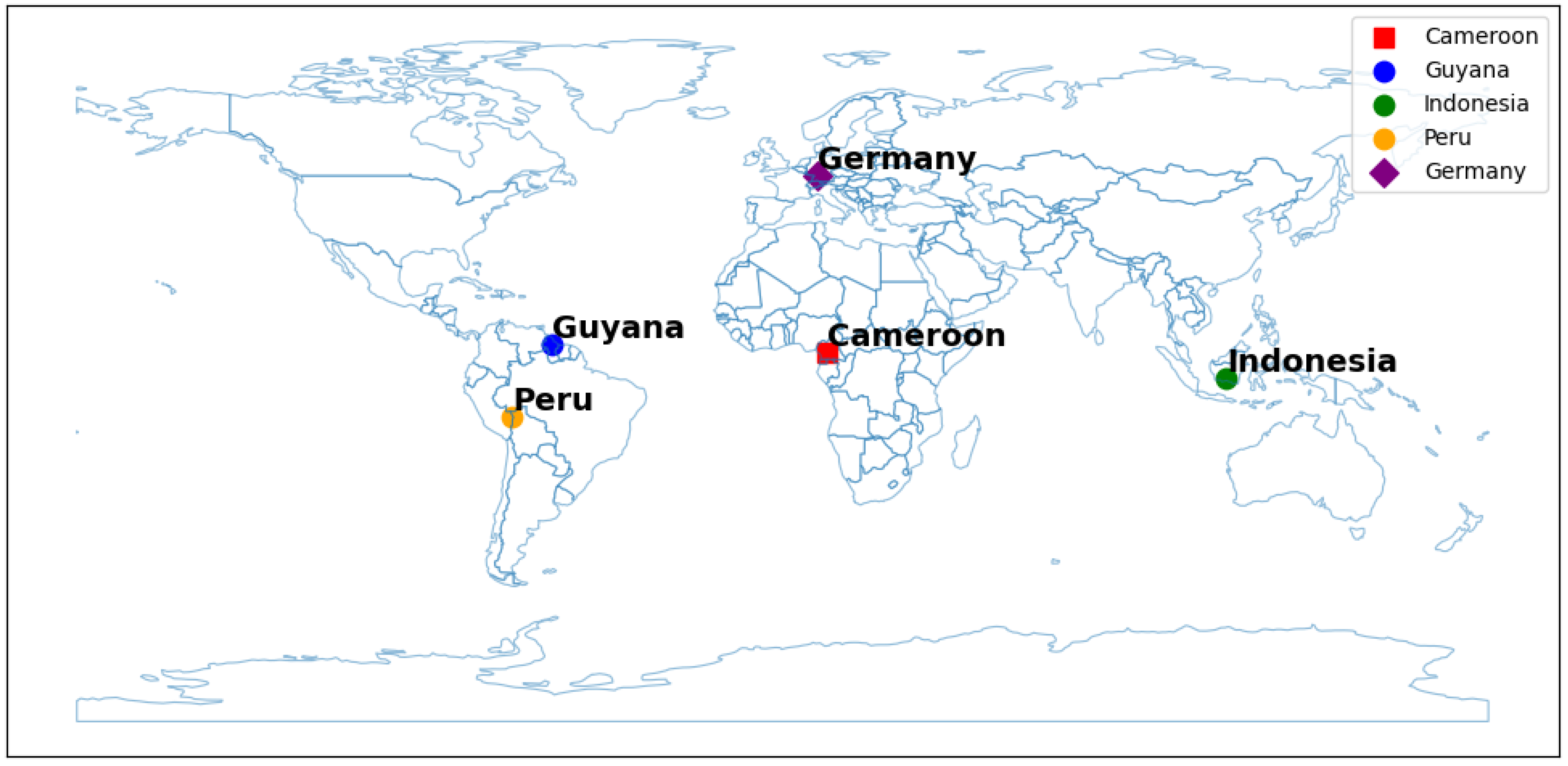
This study relies on open-source data from three sources: Gonzales et al. [27], Takoudjou et al. [9], and Weiser et al. [28]. The datasets contain point cloud data from various locations, including Guyana, Indonesia, Peru, Cameroon, and Germany on a single tree level. The naming convention for the datasets is as follows: The tree point cloud data from Guyanese and Indonesian sites follow a naming convention where the first three letters of the country name are followed by a number, such as GUY01 and IND01. The Peruvian data follow the convention of using the first three letters of the site name “Madre de Dios” (South Western Amazon), followed by a number, e.g., MDD01. The Cameroon data use arbitrary ID numbers ranging from 1 to 106 to represent the trees. The German data utilize the first three initials of the full species name, followed by the plot name, to name the trees. However, for the purpose of this study, we simplified the naming convention and used only the species type name of the tree. For example, “PinSyl” represents the species name “Pinus Sylvestris”.
The wood and leaf were manually labelled in all datasets except for the German data, which we had to label manually. Specifically, Gonzales et al. [27] collected point cloud data for 29 trees from three sites: Guyana, Indonesia, and Peru. Takoudjou et al. [9] collected data from Cameroon, which included 61 trees, while Weiser et al. [28] collected data from Germany, from which we selected only five trees. The overall dataset contains point cloud data for 38 tree species across 26 genera. Along with the point clouds that are labelled with wood and leaves, Takoudjou et al. [9] and Gonzales et al. [27] also provide destructive volume information that is useful in evaluating the potential of leaf-filtering algorithms for volume estimation. Hence, the various leaf-filtering algorithms were compared using labelled point cloud data from 95 trees, of which a destructive volume was available for 90 trees.
Both the Gonzales et al. [27] and the Weiser et al. [28] datasets were acquired using a RIEGL VZ-400 3D® laser scanner, RIEGL Laser Measurement Systems GmbH, Horn, Austria with the angular resolution set to 0.35 mrad and 0.3 mrad, respectively. Takoudjou et al. [9] used a Leica C10 Scanstation, Leica Geosystems, Heerbrugg, Switzerland with the angular resolution set at 0.5 mrad. Readers interested in learning more about the data and the TLS scanning parameters used during data collection should refer to the aforementioned articles. The geographical distribution of these datasets is illustrated in Figure 1, highlighting the diverse locations covered by the study, ranging from tropical rainforests to temperate forests.
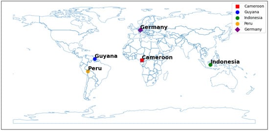
Figure 1.
Geographical distribution of the datasets utilized in this study.
Table 2 lists the datasets used, as well as dataset information pertaining to a variety of species and morphological parameters. We compared the algorithm performance across all datasets to find one that would work well regardless of the environmental variables, species, sensor configurations, data quality, and morphological details.

Table 2.
Description of dataset used in this study.
4. Methods Employed
This section encompasses various subsections that detail the approach and techniques used in the research. In Section 4.1, the focus is on the training and validation datasets. It explains the process of selecting trees from different sites for training and validation, along with the subsampling of the point cloud to create variations in data density. This allows the study to investigate the impact of density variation on the algorithms. Section 4.2 delves into specific leaf-filtering algorithms, namely, LeWoS, TLSeparation, CANUPO, and RF. These algorithms are thoroughly explained, covering various aspects such as parameter optimization, feature extraction, and selection processes. Moving forward, Section 4.3, the performance assessment subsection, details the metrics used to evaluate the effectiveness of the algorithms. It places emphasis on pointwise classification accuracy and volume comparison techniques, utilizing metrics such as overall accuracy (OA), F-score, mean absolute deviation (MAD), and mean absolute percentage deviation (MAPD). Additionally, the AdQSM model for tree reconstruction is discussed, focusing on its input parameters and experimentation with different parameter values. Collectively, these subsections provide a comprehensive outline of the methodologies employed in the study, covering dataset selection, algorithm implementation, performance evaluation, and volume estimation.
4.1. Training and Validation Dataset
For this study, we utilized two machine-learning algorithms, CANUPO and RF, which require training datasets to learn the model. To ensure fair comparison of algorithm performance, the same training dataset was used for both algorithms. Out of the total 95 trees in the dataset, 36 trees from Cameroon were selected for training, while the remaining 59 trees were used for validation, including 25 from Cameroon, 10 from Guyana, 10 from Indonesia, 9 from Peru, and 5 from Germany. All algorithms were run on this validation dataset for comparison. To investigate the impact of point cloud density on leaf-filtering algorithm performance, the original point cloud was further subsampled to lower data density by 30%, 50%, 70%, and 90%. This was accomplished by randomly removing points throughout the height of the tree. The subsampling was performed using the random subsampling option available in CloudCompare.
4.2. Leaf-Filtering Algorithms
LeWoS and TLSeparation were originally designed for leaf–wood separation, while the CANUPO algorithm primarily targeted natural scene classification. In this study, we repurposed CANUPO for leaf-filtering, thoroughly evaluating and comparing its performance in this context. Additionally, previous studies employing the RF algorithm had encountered limitations in their models [13,19]. We developed a robust RF model that not only surpasses the performance of other algorithms but also demonstrates its versatility. Importantly, while our RF model was trained on a subset of the Cameroon dataset, we validated its effectiveness across a diverse range of datasets, including the remaining portion of the Cameroon dataset and datasets from other sites, such as Guyana, Indonesia, Peru, and Germany, highlighting its universal applicability.
4.2.1. LeWoS
LeWoS is a MATLAB-based algorithm that requires MATLAB programming software or the MATLAB Runtime version. We used MATLAB 2022b to run LeWoS in this study. The parameter verticality needs to be optimized for the algorithm. This parameter varies with changes in point cloud density or site, indicating the need for manually leaf-filtered reference data to optimize the parameter for a particular dataset.
To obtain a generalizable value that is applicable to all study areas and point cloud densities, we used the default value of 0.125 for verticality. However, we also investigated the impact of optimizing this parameter on the algorithm’s performance, and the results are presented in Section 5.2.1. Specifically, we considered 11 trees from five different sites (including three trees from the Cameroon dataset and two trees from each of the other four sites) to observe the effect of optimization.
To find the optimal value of verticality for each site, we ran the algorithm for a set of verticality values, creating a ramp of 0.1 to 0.3 with a step size of 0.25. This resulted in nine output combinations for each tree. We used the F-score to define the best value of verticality for each site. For more information on the impact of optimization, please refer to Section 5.2.1.
4.2.2. TLSeparation
TLSeparation is a Python library that can be easily installed using pip, a package manager for Python. For this study, we used the generic_tree script to separate leaves and wood, following the same approach as described by the developers in their published paper [20]. The script has three parameters that need to be optimized: the set of knn values used for neighbourhood search in the GMM classification step, the voxel size used in both steps of shortest path analysis, and the steps to retrace for path retrace classification. To optimize these parameters, we followed the methodology suggested by [20], which involves evaluating the overall accuracy of 10 pseudo-random combinations of these values. However, as with LeWoS, manually leaf-filtered data are required for optimization.
To compare the performance of TLSeparation with other algorithms, default values were used for these input parameters. The impact of optimization for TLSeparation is also presented in Section 5.2.2. We used the same dataset as for the optimization of LeWoS, which included 11 trees from five different sites. The pseudo-random combinations were obtained from the suggested possible values in Table 5 of Ref. [20]. The algorithm was run for a set of parameter values resulting in ten combinations of output for each tree, and the F-score was used to determine the optimal combination for each site. For more information on the impact of optimization, please refer to Section 5.2.2.
4.2.3. CANUPO
CANUPO, integrated as a plugin within CloudCompare, follows a two-phase approach involving training and classification. During the training phase, it leverages a labelled point cloud dataset. Once trained, the model can be saved and applied for classification tasks on new data.
In addition to the point cloud of two separate classes, a set of values for computing multi-scale descriptors are taken as input. For this study, we defined the ramp of scale from 0.1 to 1 with a step size of 0.1, resulting in a list of values [0.1, 0.2, 0.3, 0.4, 0.5, 0.6, 0.7, 0.8, 0.9, 1.0]. Furthermore, there is an option to choose the number of core points on which the descriptors will be computed. To achieve the highest possible accuracy, we used all the points from the original point cloud. When applying the trained classifier to the unlabelled point cloud, we also chose to use all the points in the computation of the descriptors.
4.2.4. Random Forest (RF)
When implementing the Random Forest (RF) algorithm, it is important to specify two key parameters: the number of classification trees () and the number of input features () used at each node [19,29]. Increasing the number of generally improves model accuracy until convergence is reached [19]. In our study, we kept the number as 100 as no major difference was observed on further increase in the number. Another parameter, was fine-tuned by evaluating the best F-score computed on the test dataset.
Feature Extraction
Feature extraction is a crucial step in machine-learning algorithms, especially when dealing with high-dimensional data such as 3D point clouds. The features extracted should be able to capture the linear, planar, or volumetric structures of the point cloud, as well as other geometric properties of the data. In this study, we extracted 3D point features based on the covariance matrix computed within a local 3D neighbourhood. The features were calculated on spherical neighbourhoods at various radius sizes, as shown in following paragraphs, to explore different responses in function to different geometric properties.
The use of a multi-scale approach for feature extraction is important as it allows the features to capture different aspects of the tree’s geometry at various scales. Different radii were tested to explore different responses in function to different geometric properties of the tree. In total, a set of 22 distinctive geometric features including the relative height were calculated for each 3D point cloud. This feature set provides a comprehensive representation of the 3D point cloud that can be effectively used in a random forest classifier for the classification of leaf and wood.
It is essential to note that, while all computed geometric features are obtainable through CloudCompare tools, we prioritized computational efficiency and aimed for a streamlined workflow in the RF model implementation. Hence, we utilized the jakteristics library in Python, leveraging Cython for faster computations compared to CloudCompare.
Feature Selection
Feature selection is the process of selecting a subset of independent features that can be used to train the model with minimum compensation on the performance and to classify the entire point cloud. In our study, we used feature selection to reduce the dimensionality of the data and improve the model’s interpretability. In this study, a threshold value of 0.05 was used to select the most important features, and a threshold of 0.03 was used to further refine the features.
First, we trained the model on a small dataset containing point cloud along with the computed features of 10 trees. Out of the total 22 geometric features, we chose those features that were giving the feature importance value of greater than 0.05. This was carried out first by considering the neighbourhood radius of 0.1 m, and then 0.2 m. We then extracted small number of features by putting threshold value of 0.05 on feature importance value extracted from both neighbourhood radius. After extracting a small number of features that are significant in differentiating the leaf and wood, we considered the effect of neighbourhood radius by adopting a multi-scale approach. We trained the model from 10 trees by considering the small number of important features extracted from the first model for different neighbourhood radius of 0.1 m, 0.2 m, 0.4 m, 0.6 m, 0.8 m, and 1.0 m. In addition to the geometric features, we also incorporated relative height, which represents the z-value of points above the ground level, as an additional feature in our analysis. By incorporating relative height as a feature, we aimed to enhance the accuracy and effectiveness of our RF model in distinguishing and filtering the wood and leaf points. Next, we took a threshold value of 0.03 on the feature importance in order to extract fewer ad hoc features (multi-scale geometric and normalized height) that can be used to train the final model.
4.3. Performance Assessment
We assessed the algorithms’ ability to distinguish leaf and wood components in a tree point cloud using pointwise classification accuracy, as evaluated by overall accuracy (OA) and F-score. We also compared the volume estimation from a leaf-filtered point cloud by each algorithm with the destructive volume by reporting mean absolute deviation (MAD) and mean absolute percentage deviation (MAPD).
4.3.1. Pointwise Classification Accuracy
Pointwise classification accuracy measures how accurately individual points in the point cloud are classified as either leaf or wood. Table 3 presents the confusion matrix for each algorithm, showing the number of true positives (TPs), false positives (FPs), false negatives (FNs), and true negatives (TNs). TPs and FPs represent the correctly and incorrectly classified wood points, respectively, while TNs and FNs represent the correctly and incorrectly classified leaf points, respectively.

Table 3.
Confusion matrix for pointwise classification accuracy assessment, where TP, FP, FN and TN represent True Positives, False Positives, False Negatives and True Negatives, respectively.
Overall accuracy is the percentage of correctly classified points out of all the points in the point cloud. F-score combines precision (the proportion of correctly classified positive points out of all classified positive points) and recall (the proportion of correctly classified positive points out of all actual positive points) and is calculated twice to report both wood and leaf classes.
The precision and recall formulae shown are for computing the F-score of wood. For computing F-score of leaves, TN, FN, and FP are substituted for TP, FP, and FN, respectively, in the precision and recall formulae.
4.3.2. Volume Comparison
Tree reconstruction was performed using the AdQSM model, which is a 3D tree reconstruction algorithm that estimates the wood volume of a tree based on the wood point cloud. Two important parameters, height segmentation (HS) and cloud parameter (CP), were used as inputs in the modelling process. HS represents the height of each segment of the point cloud, whereas CP represents the point cloud’s extraction rate. The authors of the AdQSM model recommend using the default value of CP for reconstructing a single tree, while suggesting that different values of HS (such as 0.5, 0.6, 0.7, 0.8, 0.9, and 1.0) should be experimented with. The resulting average volume from these experiments should be reported as the outcome of the tree reconstruction. We obtained our tree reconstruction results by adhering to the suggested methodology.
We opted to utilise the AdQSM model because of its high reported accuracy, ease of application, and computational efficiency in reconstructing tree point clouds. In their published paper [26], the authors compared the performance of AdQSM with that of TreeQSM, another QSM model, and found that AdQSM outperformed TreeQSM in terms of accuracy and speed. Furthermore, the AdQSM model simplifies the process even more by not requiring extensive optimization of a large set of parameters, as was the case with TreeQSM.
We filtered the point cloud using each algorithm and compared the volume estimated from the resulting leaf-filtered point cloud with the destructive volume using AdQSM. We calculated MAD and MAPD to assess each algorithm’s volume extraction. In Equations (5) and (6), “” and “” are self-explanatory terms representing the volume computed through AdQSM tree reconstruction for a specific algorithm (LeWoS, TLSeparation, CANUPO, or RF) and the reference destructive volume for each tree, respectively.
5. Results
5.1. Feature Selection (for RF Model)
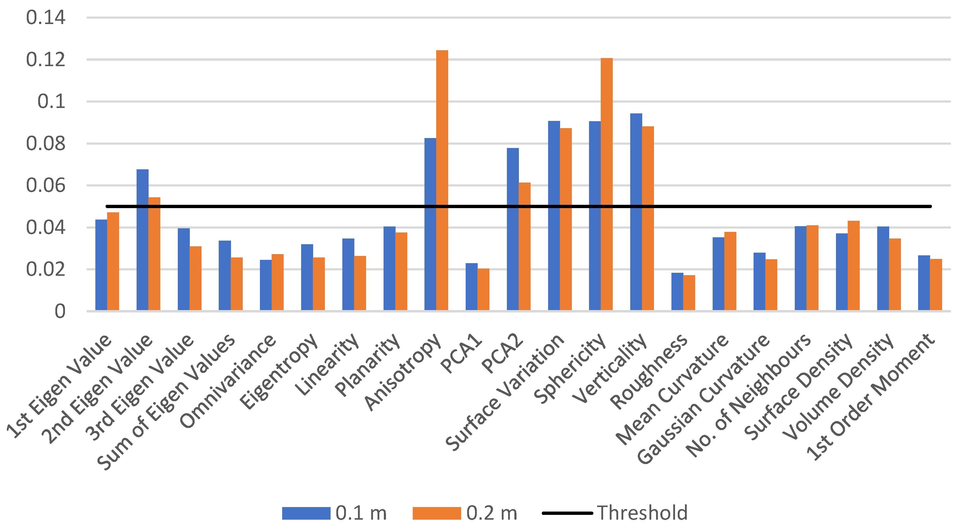
To differentiate between the wood and leaf points at a specific radius of 0.1 m, we first extract the features listed in Table 4 and train the model on a small dataset of 10 trees. The feature importance value is reported, and the process is repeated for a neighbourhood radius of 0.2 m. The feature importance values for both test models are shown in Figure 2. The results indicate that the prioritized features remain the same for different neighbourhood radii. A threshold of 0.05 is applied to the feature importance value, resulting in the selection of six important features: the second eigenvalue, anisotropy, PCA2, surface variation, sphericity, and verticality.

Table 4.
Summary of extracted features and their significance for leaf–wood classification. The features are categorized into distinct groups, each contributing to the characterization of the point cloud’s geometric properties. The significance and formulae of individual features are outlined, encompassing covariance features, density features, moments, roughness, curvature features, and z-value (relative height). These features collectively form a robust set for training the RF classifier.
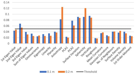
Figure 2.
Feature importance values for neighbourhood radii of 0.1 m and 0.2 m. The graph shows the feature importance values for a test RF model trained on a small dataset of 10 trees, highlighting the major contributions made by the features for two different neighbourhood radii: 0.1 m and 0.2 m. Features with importance values above the threshold of 0.05 are selected for further feature selection process.
These features play pivotal roles in distinguishing between wood and leaf points. The second eigenvalue and PCA2 provide insights into point distribution and orientation, aiding in the identification of leaf and wood point clouds with differing distributions. Anisotropy measures the non-uniformity or directionality of point distribution, facilitating pattern identification. Surface variation captures variations in surface geometry, contributing to discrimination between wood and leaf points. Sphericity indicates how spherical or elongated the point distribution is, offering information about the overall shape characteristics. Verticality is crucial in forestry applications, helping identify point orientation with respect to the vertical axis.
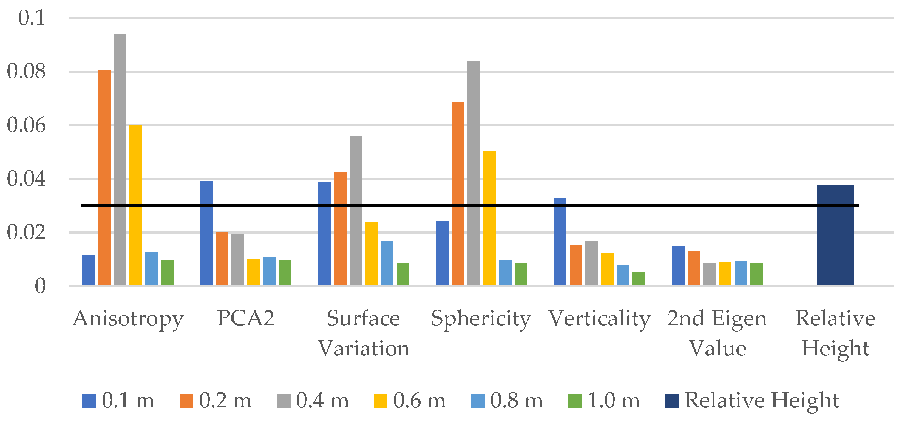
Next, we investigate the effect of multi-scale by training the model on six previously selected features for different neighbourhood radii of 0.1 m, 0.2 m, 0.4 m, 0.6 m, 0.8 m, and 1.0 m, resulting in a total of 36 features. Additionally, we include the relative height of each point as a feature, bringing the total number of features to 37. We then applied a threshold of 0.03 on the feature importance values to select a smaller set of 12 ad hoc features, as shown in Figure 3. The final RF model is trained using these 12 ad hoc features.
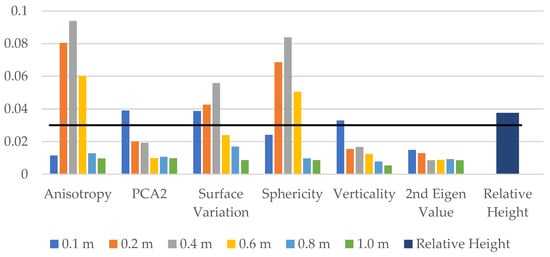
Figure 3.
Feature importance values for multi-scale analysis. The graph displays the feature importance values for a test RF model trained on a dataset with varying neighbourhood radii (0.1 m, 0.2 m, 0.4 m, 0.6 m, 0.8 m, and 1.0 m) and an additional feature representing the relative height of each point. Features with importance values greater than the threshold of 0.03 are selected for training the final RF model.
5.2. Effect of Parameter Optimization
5.2.1. LeWoS
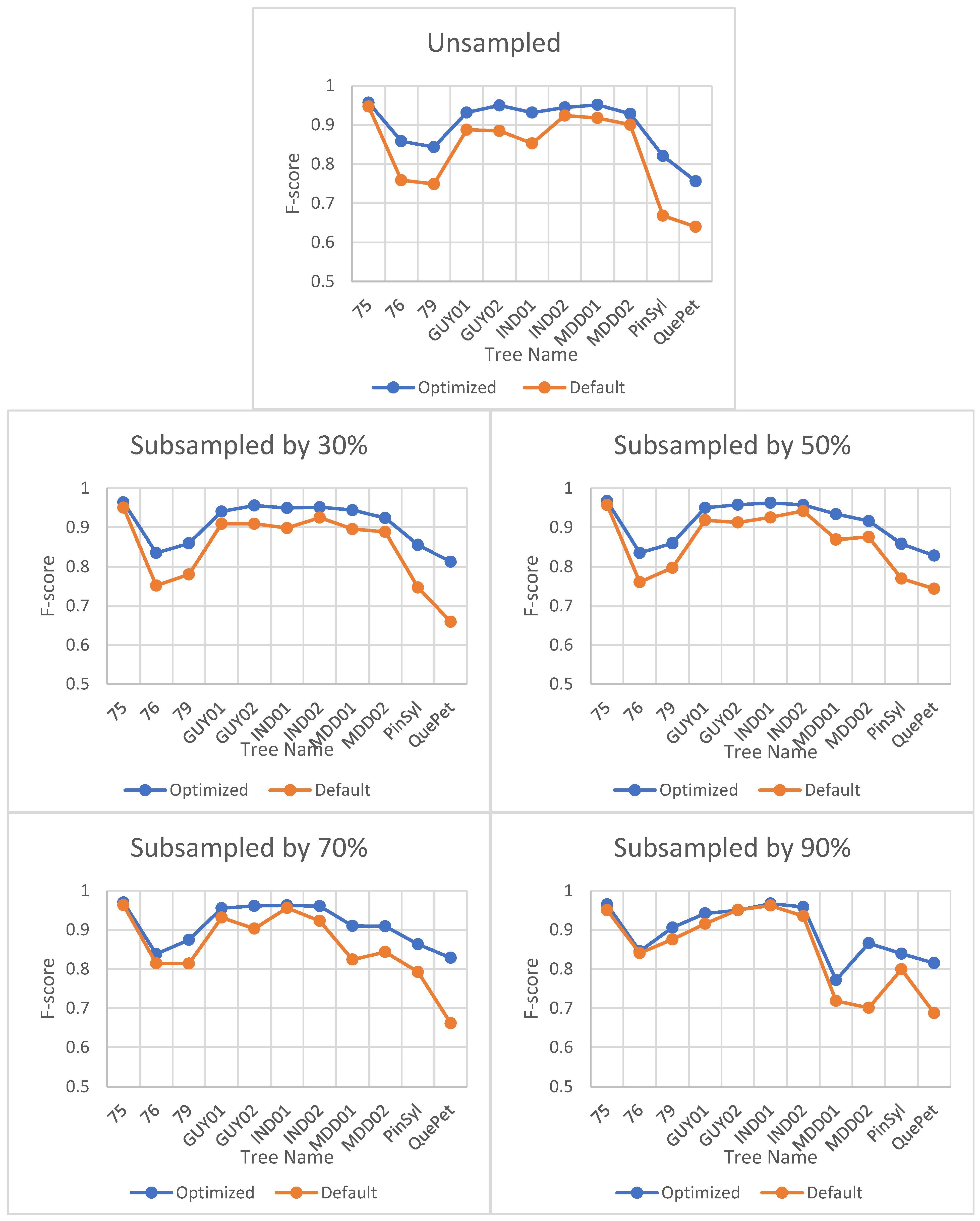
The impact of optimization on the F-score is minimal and does not vary significantly for different sites or point cloud densities. However, the optimal value of the verticality parameter, which is the only input parameter for LeWoS, can vary depending on the site or point cloud density. Table 5 shows the optimized value of verticality for each site and its corresponding point cloud density. Figure 4 illustrates the impact of optimization on the F-score.

Table 5.
Optimal values of verticality for LeWoS algorithm on different sites and point cloud densities.
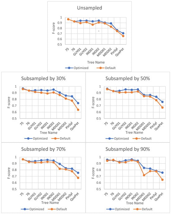
Figure 4.
Effect of parameter optimization on F-score for LeWoS at different point cloud densities. The horizontal axis represents the tree names selected from different datasets, and the naming convention for the trees can be understood as defined in Section 3.
5.2.2. TLSeparation
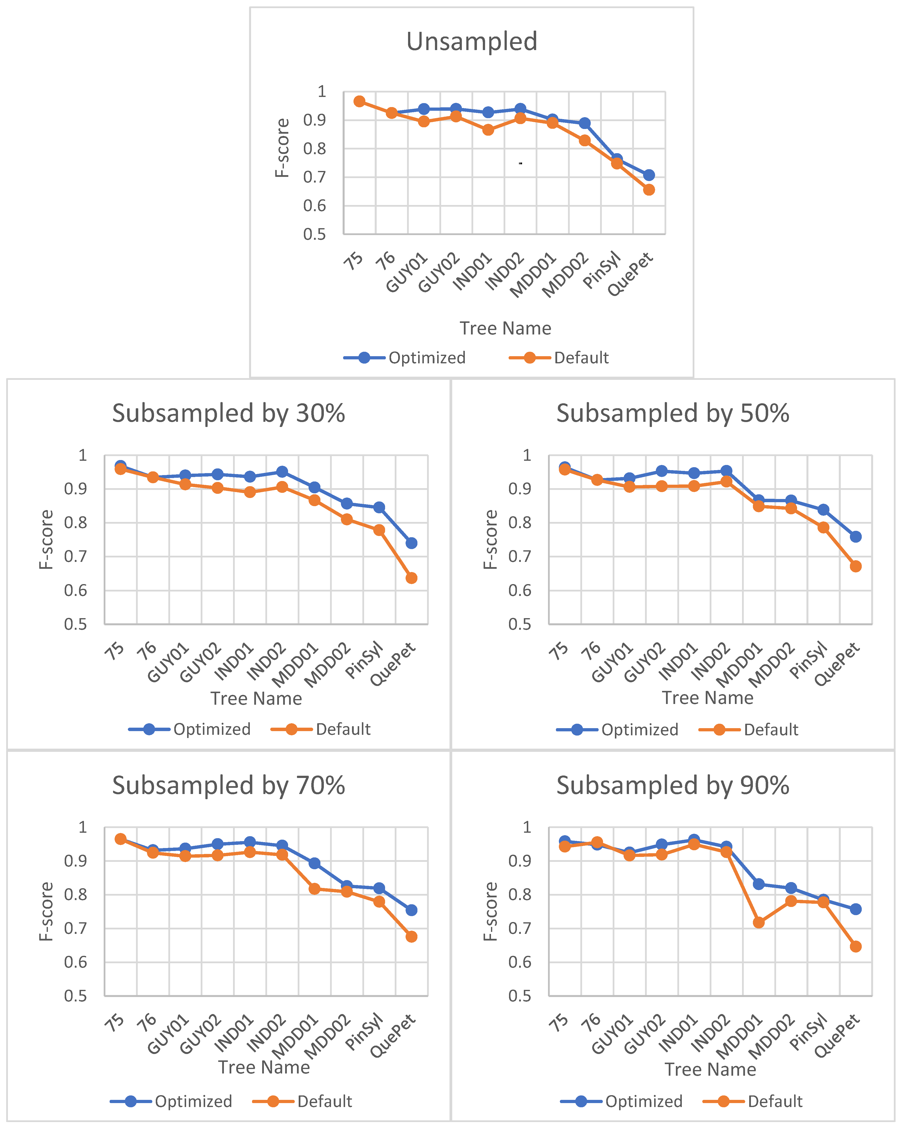
Optimizing the parameter values for TLSeparation had a significant impact on the algorithm’s performance, as seen in Figure 5. The F-score improved significantly when using optimal parameter values compared to default values. However, the effect of optimization decreased with decreasing point cloud density, as shown in Figure 5.
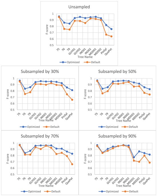
Figure 5.
Impact of optimization on F-score for TLSeparation at different point cloud densities. The horizontal axis represents the tree names selected from different datasets, and the naming convention for the trees can be understood as defined in Section 3.
Interestingly, the optimal parameter combination for a particular site was also found to be optimal for all tested point cloud densities, as shown in Table 6. This suggests that the optimal parameter combination is site-specific rather than density-specific.

Table 6.
Optimal parameter combination for TLSeparation at different sites and point cloud densities. The parameters, including KNN values and voxel size, are outlined for different subsampling scenarios. The site-specific and density-agnostic effectiveness of these optimal parameter values highlights their significance in achieving robust performance. Refer to the combination number for specific parameter values.
5.3. Pointwise Classification
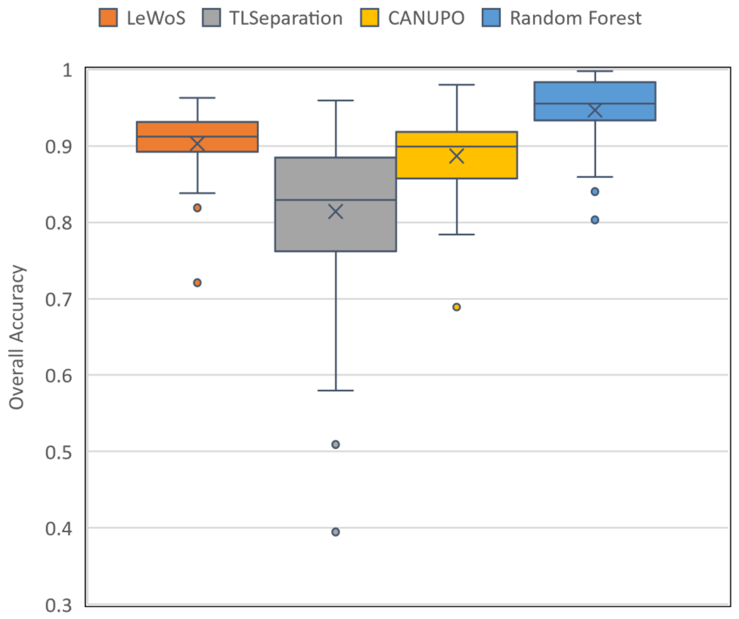
The performance of the four algorithms for pointwise classification was evaluated using the validation dataset, and the results are summarized in Table 7. The per-tree accuracy ranged from 0.72 to 0.96 for LeWoS, 0.39 to 0.96 for TLSeparation, 0.69 to 0.98 for CANUPO, and 0.8 to 0.99 for RF, with mean values of 0.9, 0.81, 0.89, and 0.95, respectively. The box and whisker plot in Figure 6 shows the distribution of the per-tree accuracy for all four algorithms. For LeWoS, the outlier and lowest value of the whisker were from the Peruvian and Guyanese sites, respectively, while for TLSeparation and CANUPO, these values were from the Cameroon data but with different trees. For RF, the two outliers and lowest value of the whisker were all from the German data. The highest accuracy was obtained from the Indonesian site for all algorithms except RF, which had the highest accuracy from the Peruvian site. The F-score for wood and leaf were very close to each other for all algorithms, with a larger value of F-score obtained for leaf except in TLSeparation. The lowest accuracy values were achieved for smaller trees with a lower DBH in all algorithms except LeWoS.

Table 7.
Assessment metrics for pointwise classification of four algorithms on the validation dataset.

Figure 6.
Box and whisker plot of per-tree accuracy for the four algorithms evaluated on the validation dataset. The box displays the quartiles for 25% to 75% of the overall accuracy, with the mean accuracy represented by a cross marker and the median accuracy shown by a horizontal line inside the box. Outliers are denoted by individual dots.
5.4. Volume Comparison
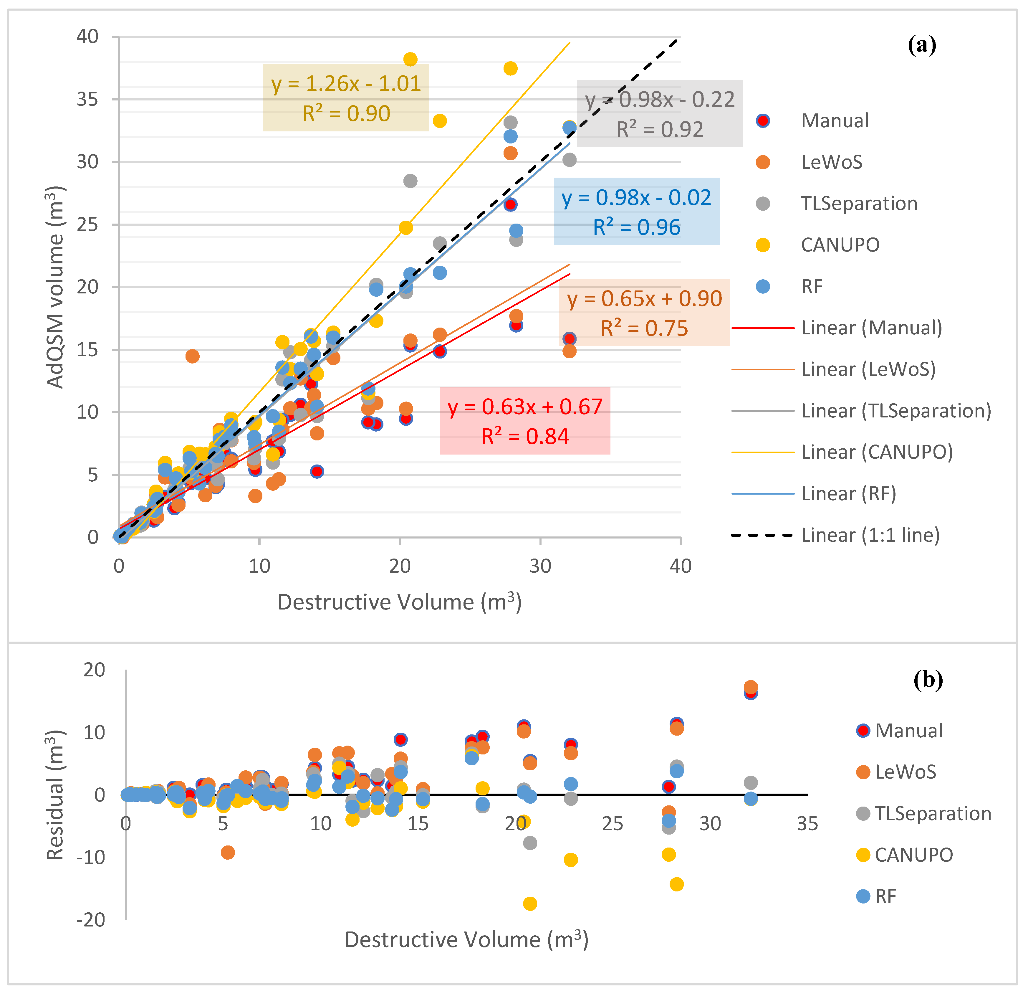
The leaf-filtered point clouds generated by the different algorithms were used as input for volume extraction in AdQSM. Additionally, manually leaf-filtered point cloud data were also used for comparison. Two trees exhibited unexpectedly large volumes and deviated from the expected range, making the plot difficult to interpret. To address this issue, these two trees were filtered out, and the resulting plot of the remaining trees is presented in Figure 7a. Additionally, Figure 7b shows the residual values for each tree.
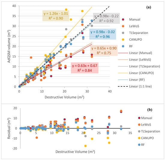
Figure 7.
Volume comparison and residual analysis for different algorithms and manually filtered point cloud data. (a) Volume comparison of remaining trees after filtering out two trees with large volumes. Dotted black diagonal line represents the 1:1 line. (b) Residual values for remaining trees, indicating deviation from destructive volume.
In Figure 7, it can be seen that AdQSM generally underestimates the volume, as indicated by the manually leaf-filtered regression line with a slope value of 0.63. All algorithms, except CANUPO, underestimate the volume with slope values smaller than 1, as shown in Figure 7a. RF and TLSeparation perform the best, as they are near the 1:1 line with a slope value of 0.98 and coefficient of regression value (R2) of 0.96 and 0.92, respectively, in Figure 7a. CANUPO and LeWoS yield slope values of 1.26 and 0.65, respectively, with their corresponding R2 values of 0.9 and 0.75.
Among all the algorithms, LeWoS performs the worst in the volume comparison, giving an underestimated value with an R2 value of 0.75. Furthermore, LeWoS has the highest value of MAPD at 30.72%, while RF has the smallest value of MAPD and MAD at 12.77% and 1.78 m3, respectively.
It is also visible that the residual values are high for trees giving larger volumes (Figure 7b). Furthermore, RF is showing the smallest residual values, almost close to the zero-line, indicating the least deviation among all of the algorithms, while TLSeparation is giving the second-least. On the other hand, LeWoS and CANUPO are showing significant deviation from the destructive volumes.
5.5. Effect of Point Cloud Density
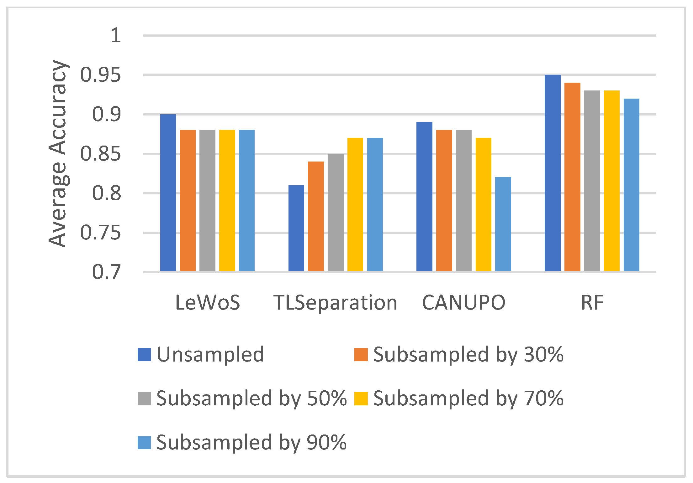
To study the effect of the point cloud density on the performance of the algorithms, we subsampled the original point cloud by 30%, 50%, 70%, and 90% and computed the average overall accuracy on the validation dataset for each case. The results are shown in Figure 8. Surprisingly, we observed no major effect on separating the wood and leaf points when the point cloud density decreased, which holds true for all the algorithms. However, the overall accuracy decreased slightly for all the algorithms except TLSeparation. This is consistent with the findings in Section 5.2.2, where we saw that parameter optimization had a greater impact on accuracy when the point cloud density was high.
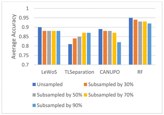
Figure 8.
Effect of point cloud density on overall accuracy for wood and leaf separation.
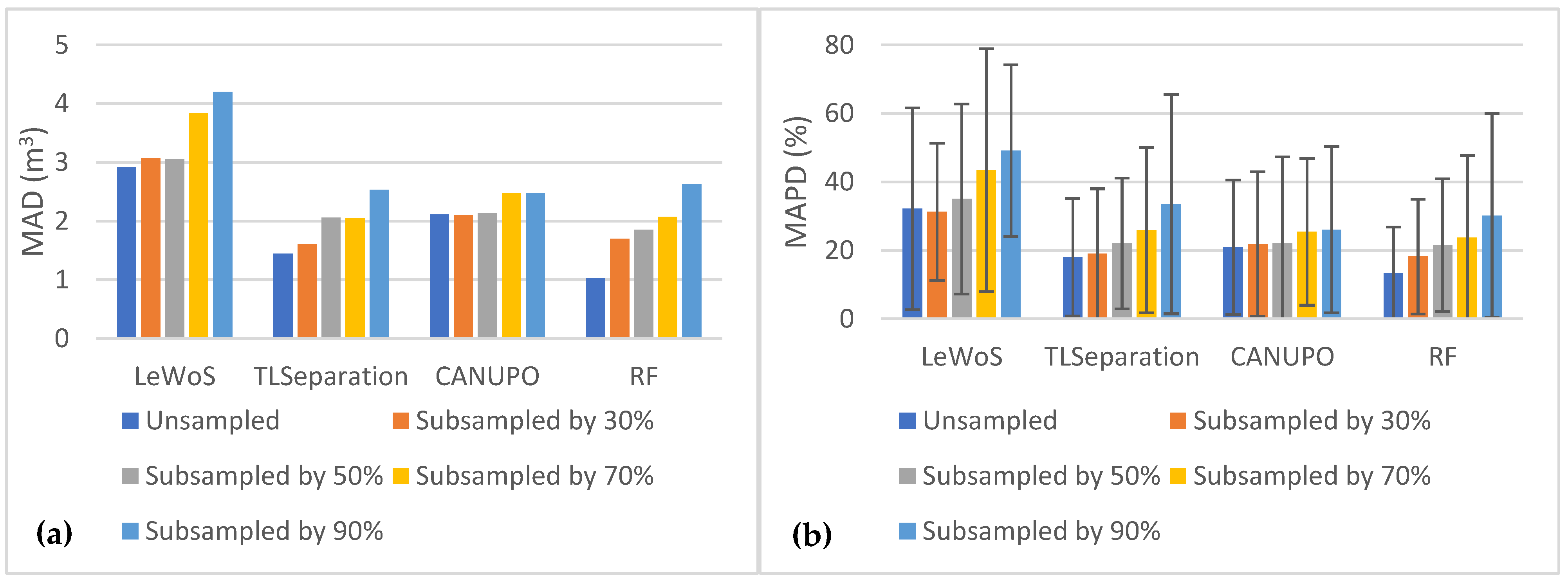
We also evaluated the algorithms’ performance in terms of volume comparison by plotting the MAD and MAPD values for each subsampling case in Figure 9. Figure 9a represents the MAD values for all the algorithms, while Figure 9b represents the MAPD values. It is evident from the plots that both MAD and MAPD increase as the point cloud density decreases, with all algorithms exhibiting a similar trend. However, CANUPO shows the least sensitivity to changes in point cloud density. In contrast, LeWoS performs the worst in each scenario, with MAPD values ranging from 32.14 ± 29.45% for the original point clouds to 49.14 ± 25.06% for the 90% subsampled point clouds. RF shows the least MAD and MAPD for all point cloud densities except for the 90% subsampled point clouds, in which CANUPO gives slightly lower values than RF.
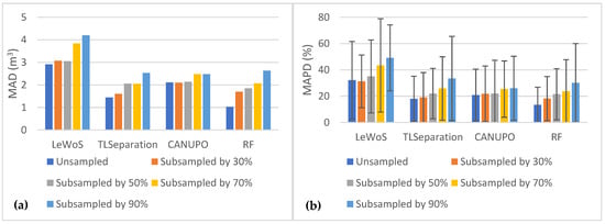
Figure 9.
The effect of point cloud density on MAD and MAPD between destructive and estimated volumes: (a) MAD values for all algorithms at different point cloud densities; (b) MAPD values for all algorithms at different point cloud densities.
5.6. Computational Efficiency
The computational efficiency of the four algorithms was assessed on a machine running the Ubuntu 18.04.6 LTS operating system, equipped with an Intel(R) Xeon(R) Gold 5218 CPU @ 2.30GHz processor, Intel Corporation, Santa Clara, CA, USA and 125 GB of memory. The algorithms were implemented in different programming languages: LeWoS in MATLAB, TLSeparation as a Python module, CANUPO originally written in C++ and also available as a plugin in the open-source software CloudCompare, and RF as a machine-learning model trained and classified using scikit-learn in Python.
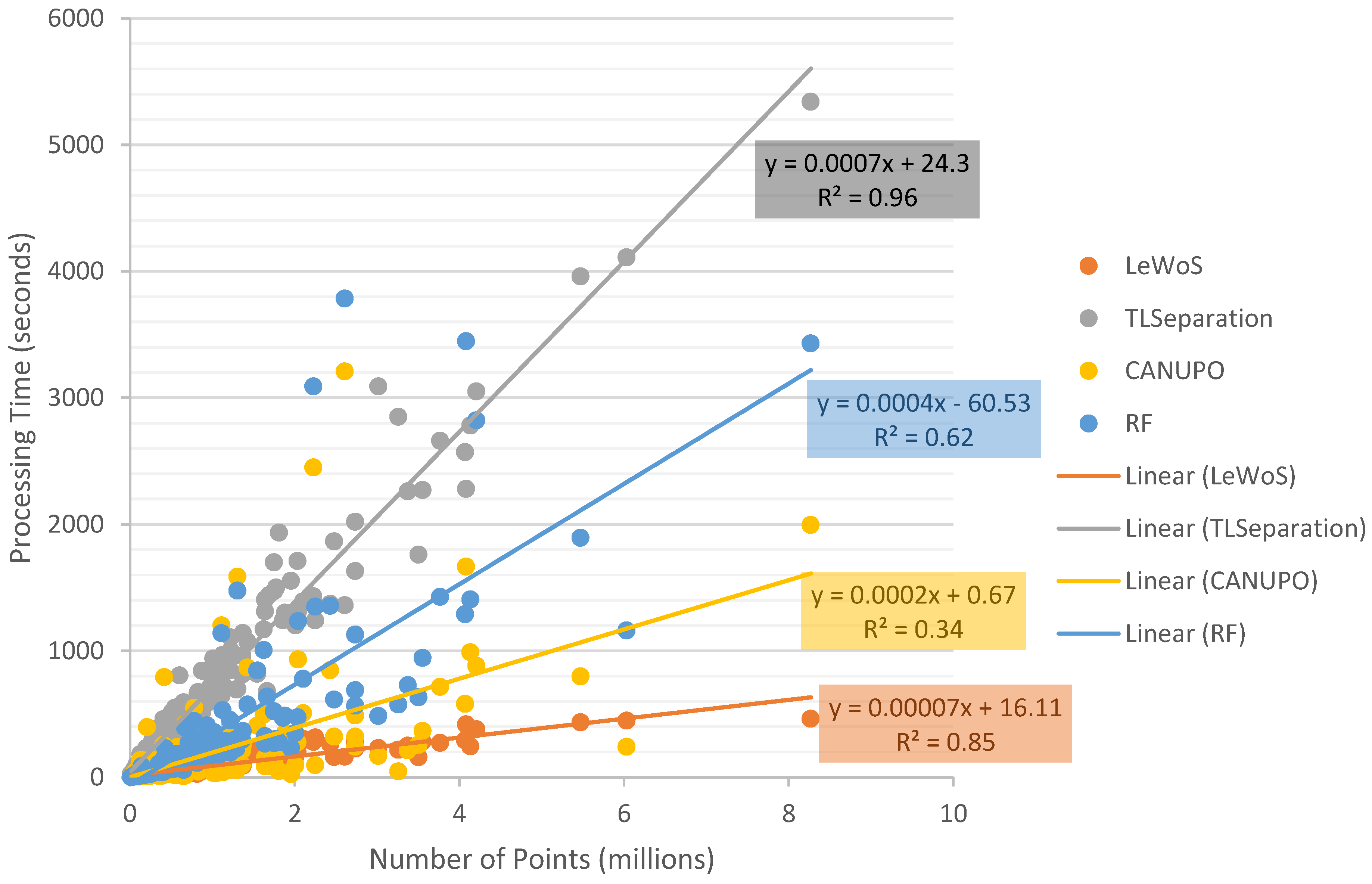
The processing time for classifying the point cloud into wood and leaf was measured for each algorithm using a dataset of 295 trees. The dataset included an unsampled validation set of 59 trees and subsampled variations of 30%, 50%, 70%, and 90%. The results of the processing time are shown in Figure 10.
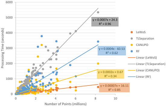
Figure 10.
Processing time required by each algorithm to classify point clouds into wood and leaf against the total number of points for each tree.
Figure 10 clearly demonstrates that the processing time required to classify the point cloud increases as the number of points increases for all four algorithms. However, the strength of the correlation and the rate of increase in processing time differ across the algorithms.
It is important to note that the processing time only accounts for the time taken by the algorithm to separate the wood and leaf points and does not include other factors such as loading and writing the dataset, parameter tuning, optimization, training the model, training dataset selection, and loading the classifier model. However, to ensure a fair comparison among all algorithms, the time spent in calculating the 11 ad hoc features mentioned in Section 5.1 for RF was included, as other algorithms only require parameter values and the point cloud as input. Therefore, the time taken by RF, as plotted in Figure 10, represents the total time taken by the RF model to classify plus the time spent in feature calculation.
6. Discussion
In this study, we systematically evaluated four algorithms for the classification of wood and leaves in TLS point clouds. Our investigation extended beyond pointwise classification accuracy, encompassing volume comparison and computational efficiency. The findings reveal that the RF algorithm consistently demonstrated superior performance in pointwise classification accuracy, while its adaptability to small branches rendered it particularly suitable for volume estimation applications utilizing quantitative structure models. These results underscore the significance of RF-based leaf filtering for precise forest parameter estimation, promising more efficient and accurate forest resource quantification, crucial for sustainable forest management and climate change mitigation.
6.1. Evaluation Based on Pointwise Classification Accuracy
In the evaluation of the four algorithms for pointwise classification using the validation dataset, RF exhibited the highest overall accuracy with a mean value of 0.95, followed by LeWoS, CANUPO, and TLSeparation. Our validation dataset was more extensive than those employed in previous studies, and, despite a slightly lower accuracy compared to D. Wang et al. [19], our RF accuracy was higher than those mentioned in X. Zhu et al. [13]. This is possibly due to the fact that we considered the influence of the neighbourhood radius and selected multi-scale features.
The accuracy of LeWoS was close to that reported by Y. Wang et al. [2], while the accuracy of TLSeparation was lower than that reported by Vicari et al. [20]. This difference could be attributed to the impact of parameter optimization, as demonstrated in Section 5.2.2. It was found that the impact of optimization was not significant for LeWoS, while, for TLSeparation, it decreased with decreasing point cloud density (Figure 5). As a result, the accuracy of TLSeparation on unsampled data was lower than that reported by Vicari et al. [20]. Nonetheless, when the point cloud was further subsampled, the accuracy matched their reported values, indicating that adjusting the algorithm parameters may mitigate its lower accuracy on unsampled data. CANUPO showed a lower accuracy in classifying wood and leaves compared to classifying rocks and vegetation which was carried out by Brodu and Lague [22]. This is likely due to the difficulties in separating thin branches and twigs from leaves, as well as the increased obstruction to the laser hit in the crown area, which results in a lower branch density and accuracy.
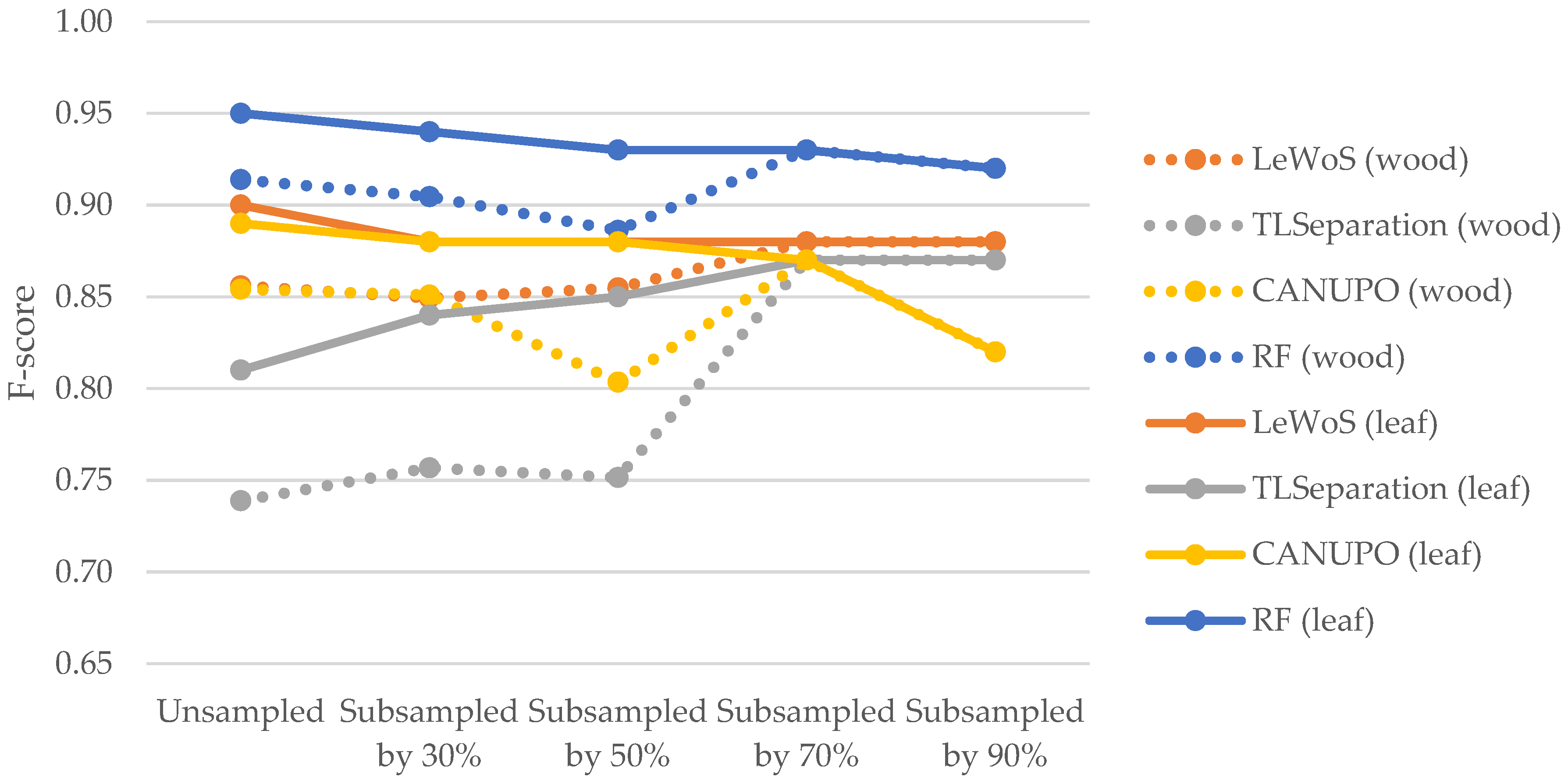
The F-scores for leaves were consistently higher than those for wood in all algorithms except for TLSeparation, which showed lower F-scores for leaves. These results suggest that the algorithms performed better at accurately classifying leaf points compared to wood points. The discrepancy in the F-scores for leaves and wood between our study and that of Vicari et al. [20] may be attributed to the impact of parameter optimization (cf. Section 5.2.2). Notably, as shown in Figure 11 TLSeparation exhibited similar behaviour to the other algorithms when the point cloud density was further subsampled, with the F-scores for wood and leaf becoming equal when the point cloud was subsampled by 70% or more. This suggests that adjusting the algorithm parameters could mitigate its lower accuracy on unsampled data.
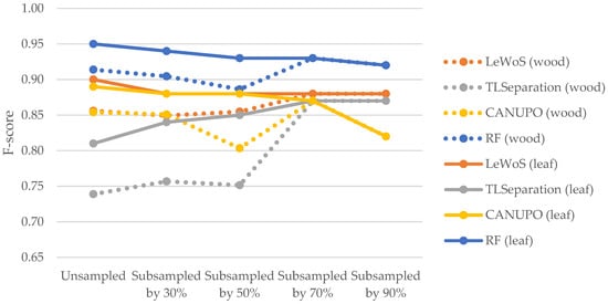
Figure 11.
Comparison of F-scores for wood and leaf points across different algorithms at varying point cloud densities. The dotted line represents the F-score values for wood points, while solid line represents the F-score values for leaf points.
TLSeparation and CANUPO exhibited the lowest accuracy values for smaller trees with a lower DBH, while RF and LeWoS demonstrated resilience to such variations as depicted in Figure 12. This indicates that the performance of TLSeparation and LeWoS decreases for smaller trees, whereas LeWoS and RF remain relatively independent of DBH.
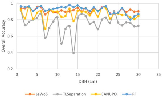
Figure 12.
Differential impact of tree size (DBH) on pointwise classification accuracy.
Overall, our findings indicate that RF outperforms the other algorithms in terms of pointwise classification accuracy, followed by LeWoS, CANUPO, and TLSeparation. It is worth noting that we utilized the LeWoS and TLSeparation algorithms directly without any optimization, as optimization requires manual wood–leaf separation work before applying them to the entire new dataset. Additionally, the impact of subsampling the data is not significant in terms of pointwise classification, which is true for all algorithms.
6.2. Evaluation Based on Volume Comparison
The evaluation of the algorithms’ volume estimation performance was conducted based on comparing the results with the destructive volume measurement. As shown in Figure 12, the algorithms performed better at accurately classifying leaf points than wood points, resulting in higher F-scores for leaves. This suggests that the algorithms are more likely to misclassify leaf points as wood, resulting in Type-1 errors or false positives. As a result, the input point cloud to the AdQSM algorithm would contain more wood points than actual wood points, including misclassified leaf points as wood points, as shown in Figure A1.
Since the AdQSM algorithm fits a model to the point cloud, a higher number of wood points in the input point cloud would cause an overestimation of volume. However, Figure 7 indicates that AdQSM underestimates the volume when fitted to a manually leaf-filtered point cloud. This underestimation is attributed to the AdQSM fitting method, as its linear fitted slope line is less than 1, indicating an underestimation of volume. Several factors contribute to this underestimation phenomenon, encompassing aspects such as the point cloud density, the occlusion of crown portions by lower branches, and the susceptibility to errors in the manual labelling of leaf and wood points, which may involve missing higher-order branch points. Hence, the overestimation due to Type-1 errors for wood points and the underestimation due to the AdQSM fitting method may compensate for each other, resulting in a volume estimate that may be closer to the destructive volume depending on the extent of misclassified leaf points as wood.
The results suggest that the LeWoS algorithm performs the worst among all the algorithms in terms of volume comparison. This is due to the fact that LeWoS misses some points from the trunk, small branches, and twigs, as illustrated in Figure A1. Furthermore, the algorithm misclassifies leaf points as wood points to a lesser extent than the other algorithms, resulting in even fewer wood points in the input to AdQSM, which may contribute to a larger underestimation of volume. In contrast, the random forest (RF) algorithm is able to classify even small branches and twigs to a greater extent while misclassifying leaf points as wood to a lesser extent than TLSeparation and CANUPO, and slightly greater than LeWoS. The improved ability of RF to classify small branches and twigs and misclassify leaf points as wood to a sufficient extent to compensate for the underestimation property of AdQSM results in a better volume extraction algorithm when assessed using destructive volume, as demonstrated by the coefficient of regression (R2) in Figure 7a, which is equals to 0.96, indicating a strong correlation between the predicted and actual volumes. Additionally, the slope value is also almost near to 1, indicating that the algorithm is not significantly overestimating or underestimating the volume, and the intercept value is almost near to zero, indicating that there is minimal bias in the volume estimation.
It is crucial to acknowledge that these outcomes may fluctuate based on the specific QSM model utilized for volume computation, as the underestimation tendency is closely tied to the AdQSM. While noting this potential variability, it is pertinent to recognize that prior research indicates that various QSM models, such as TreeQSM [8,30] developed by Raumonen et al. [31] and SimpleForest [9,10] developed by Hackenberg et al. [32], similarly exhibit underestimation tendencies. Considering RF’s adeptness in accurately classifying small branches and twigs, along with the pervasive underestimation tendencies observed in several QSM models, the volume extraction strategy centred around RF-based leaf filtering emerges as a better choice for leaf filtering in the context of volume extraction utilizing QSM models.
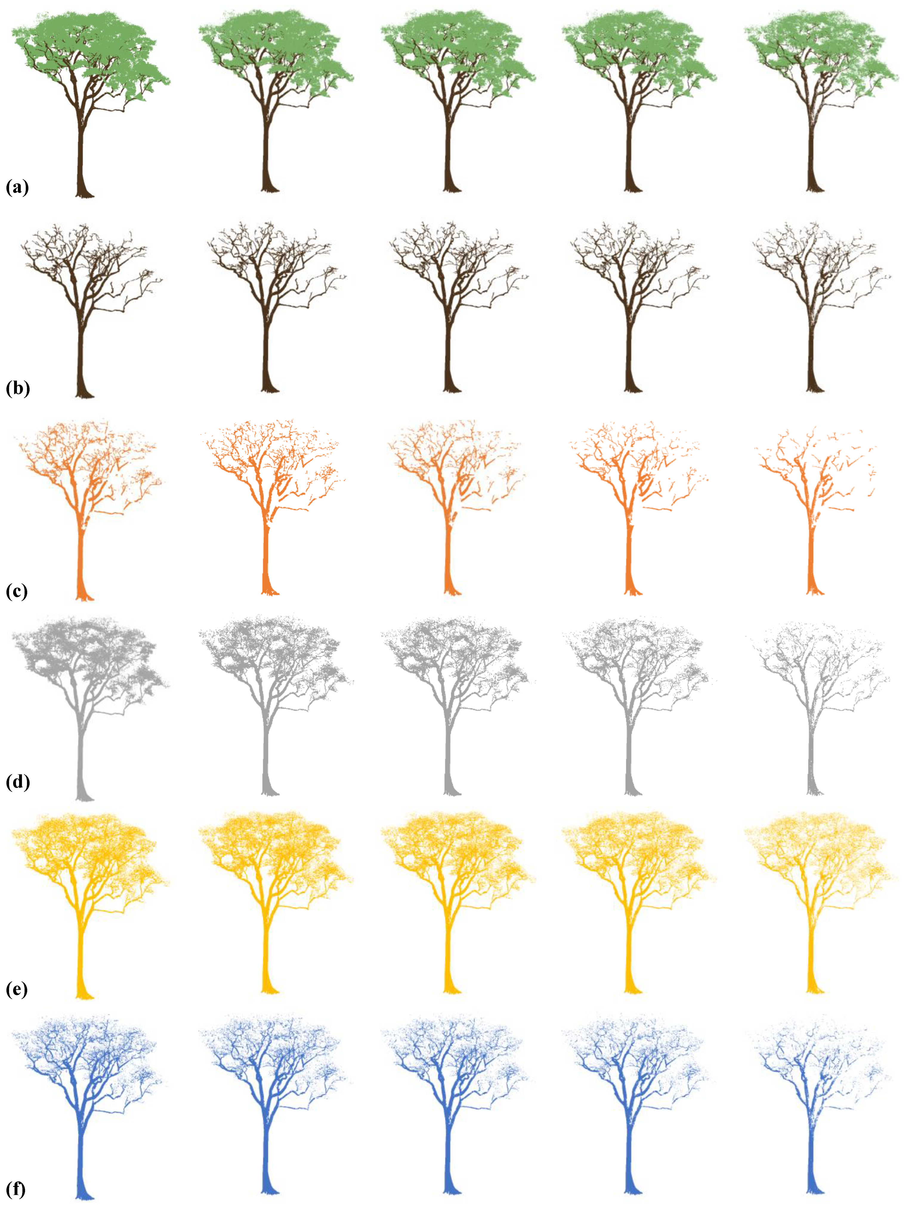
The findings of the study are indeed intriguing, particularly the fact that, even after reducing the point cloud density by 90%, there was a relatively minor reduction in the estimated volume. This is likely due to TLS capturing the major points of the trunk, which constitutes a significant portion of the total volume. Consequently, even after subsampling, there were still enough points left for the trunk to be classified as wood, as demonstrated in Figure A2. Nonetheless, there was a decreasing trend in volume extraction as the point cloud density decreased, emphasizing the importance of scanning the tree at an appropriate resolution to ensure that enough points are captured for accurate volume estimation.
Regarding the performance of the algorithms, it is noteworthy that LeWoS consistently yielded the worst volume extraction results from AdQSM among all algorithms, regardless of point cloud density, with the highest MAD and MAPD values in Figure 9. On the other hand, RF performed best for volume extraction from AdQSM among all algorithms for any point cloud density, with the lowest MAD and MAPD values in Figure 9. It is also important to mention that, although AdQSM was used for volume extraction due to its simplicity and lack of need for parameter optimization, the results may differ when using other QSM models.
6.3. Evaluation Based on Computational Efficiency
Many studies did not focus on the computational efficiency of the algorithm, except a few such as the one by Wang et al. [21], who provided information on the processing time of the LeWoS algorithm. The time taken by an algorithm to process data can vary depending on factors such as the programming language used, the system configuration, and the design of the algorithm itself, such as whether it processes the entire dataset at once or segments it for parallel computing.
The results of our evaluation showed that LeWoS was the fastest among all algorithms, while CANUPO and RF took slightly more time than LeWoS, but still within acceptable limits. On the other hand, TLSeparation was found to be the slowest, taking considerably more time to classify the data. However, our results were faster compared to those reported by Wang et al. [21], likely due to the use of a faster processor in our system.
It should be noted that computational efficiency is an important consideration in algorithm selection, as it impacts the time taken for processing large datasets, and it can vary depending on multiple factors, including hardware configuration, software implementation, and dataset characteristics. Therefore, it is essential to carefully evaluate and compare the computational efficiency of different algorithms in the specific context of the study to make informed decisions about their suitability for a particular application.
7. Conclusions
In this research, we embarked on an extensive exploration and evaluation of various algorithms designed for the crucial task of wood–leaf 3D TLS point classification. This process serves as a pivotal precursor to volume extraction through QSM. Through our comprehensive analysis and comparison, we have gained valuable insights into the strengths and limitations of different algorithms, and their performance in terms of accuracy, interpretability, and computational efficiency.
Based on our findings, it is evident that the choice of algorithm plays a critical role in achieving accurate and reliable classification results, which, in turn, impacts the accuracy of volume extraction through QSM models. Our comparison revealed that RF showed highly accurate results in separating the wood–leaf points (OA = 0.95 ± 0.04) and provided volume extraction through AdQSM models that closely aligned with the destructive volume (R2 = 0.96, slope value of 0.98), demonstrating the potential of ML in wood–leaf separation.
What makes our RF model particularly noteworthy is its consistent performance across a diverse range of datasets, highlighting its broad applicability beyond its initial training dataset, which consisted of data from 36 Cameroon trees. Remarkably, despite its training on a specific dataset, our RF model showcased exceptional robustness and consistently delivered outstanding results across datasets originating from various geographic locations, encompassing a wide spectrum of tree types and species. Furthermore, RF exhibited promising results in terms of interpretability and computational efficiency, processing 1 million points in approximately 340 s, making it a suitable choice for leaf-filtering and subsequent volume extraction. These extracted volumes can further be translated into biomass or carbon content using appropriate conversion ratios.
Among the other evaluated algorithms, LeWoS, while efficient (86 s), exhibited a lower accuracy and volume estimation. TLSeparation achieved comparable volume estimates (R2 = 0.92) but with a lower accuracy (OA = 0.81 ± 0.10) and longer processing times (724 s). CANUPO, processing in 200 s, demonstrated good efficiency but inferior volume estimation.
While we ensured a sufficiently large training and validation dataset, it is worth mentioning that ML models may perform even better with additional data. Furthermore, we did not consider deep-learning (DL) models in this study, which could be explored in future research. Additionally, the performance of the RF model could potentially be improved by incorporating radiometric features, as we only used geometric features in our study. Moreover, the effect of using different QSM models should also be taken into account in future research. Furthermore, the performance of the algorithms on other types of LiDAR data, such as UAV-LiDAR or Mobile LiDAR, could also be evaluated in future studies.
Our research contributes to the understanding of algorithm selection for wood–leaf separation, which is an intermediate step in the process of volume extraction from point cloud data captured by TLS. The insights gained from our analysis can provide valuable guidance for future research and practical applications in volume extraction through QSM models. Future research could focus on developing more robust RF models or exploring the potential of DL models in wood–leaf separation. Overall, our findings contribute to the body of knowledge in the field and provide valuable guidance for researchers and practitioners in selecting appropriate algorithms for wood–leaf separation in the context of volume extraction from point cloud data collected through TLS.
Author Contributions
Conceptualization, M.A., B.L. and M.H.; methodology, M.A., B.L. and M.H.; validation, M.A., B.L., M.H. and N.P.; writing—original draft preparation, M.A.; writing—review and editing, M.A., B.L., M.H. and N.P.; supervision, B.L., M.H. and N.P. All authors have read and agreed to the published version of the manuscript.
Funding
This research received no external funding.
Data Availability Statement
The data utilized in this study are sourced from various origins. The Cameroon dataset was originally published by [9] and can be accessed at https://doi.org/10.5061/dryad.10hq7. Additionally, the data from Guyana, Indonesia, and Peru were published by [27] and are accessible at https://doi.org/10.4121/21552084.V1. A portion of the data employed in this study, pertaining to Germany, was published by [28] and can be retrieved from https://doi.org/10.1594/PANGAEA.942856.
Acknowledgments
The authors would like to acknowledge the contributions of Gonzales de Tanago Menaca, Momo Takoudjou, and Weiser, along with their respective co-authors, for publishing the open-source data used in this study. Their valuable contribution is greatly appreciated. We would also like to express our gratitude to the reviewers for their valuable comments and suggestions that have significantly improved the quality of this manuscript.
Conflicts of Interest
The authors declare no conflicts of interest.
Appendix A
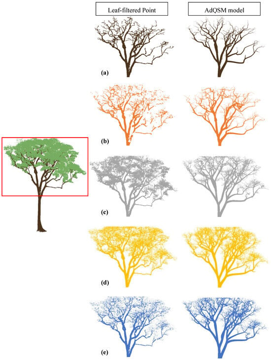
Figure A1.
Visual comparison of output from different algorithms for a tree. The left-centred image displays the whole tree point cloud with a red box highlighting the area of comparison. The middle and last columns show the resulting leaf-filtered point clouds obtained using (a) manual filtering, (b) LeWoS, (c) TLSeparation, (d) CANUPO, (e) RF, and the resulting QSM model, respectively.
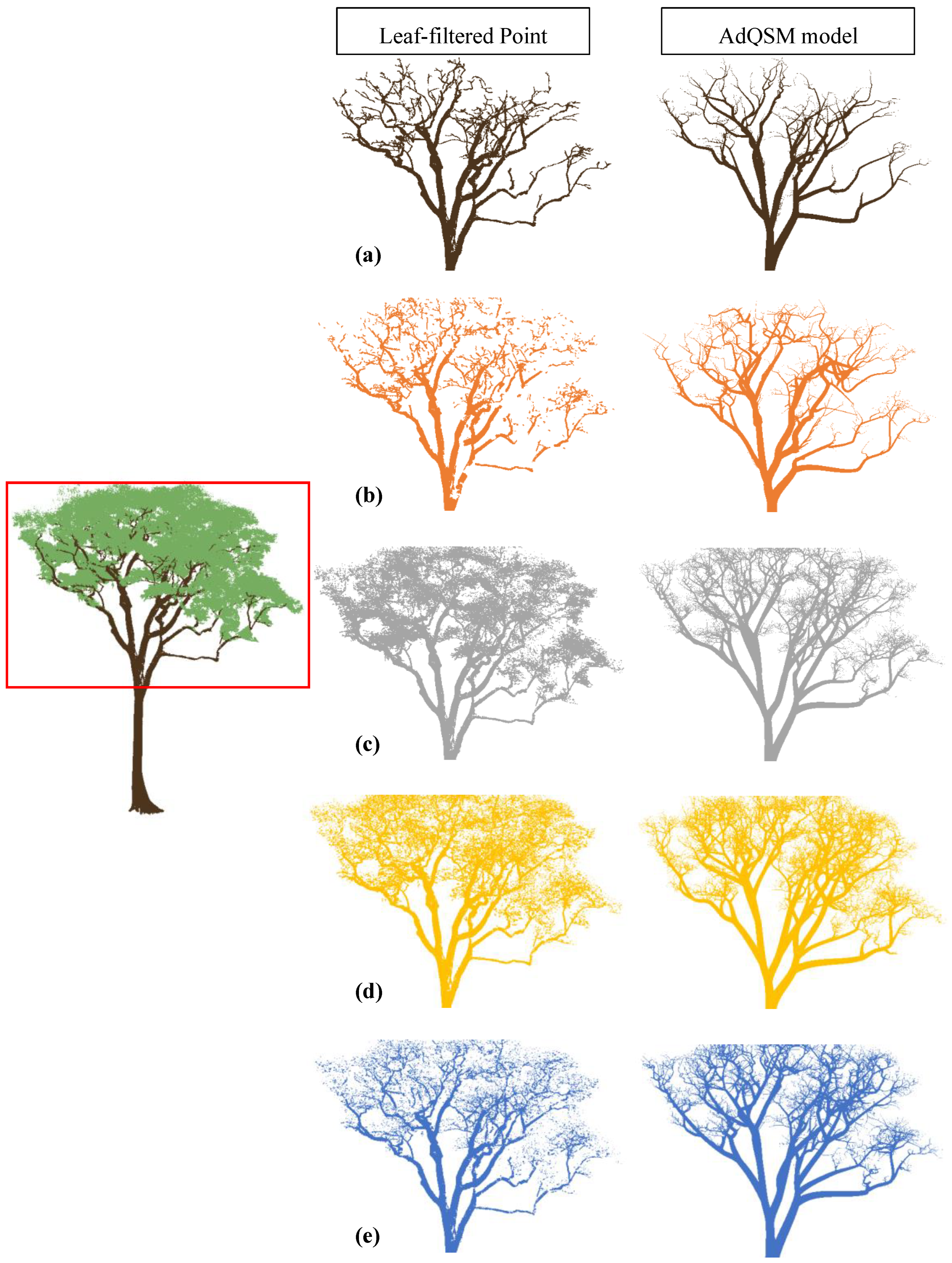
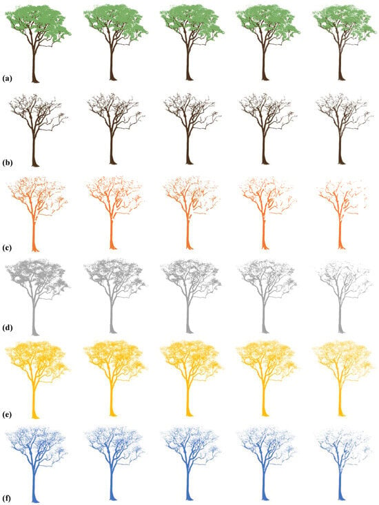
Figure A2.
Effect of point cloud subsampling on wood–leaf separation algorithms. Whole tree point cloud (a), manual leaf-filtered point cloud (b), and results of LeWoS (c), TLSeparation (d), CANUPO (e), and RF (f) at different subsampling percentages (unsampled, 30%, 50%, 70%, and 90%).
Figure A2.
Effect of point cloud subsampling on wood–leaf separation algorithms. Whole tree point cloud (a), manual leaf-filtered point cloud (b), and results of LeWoS (c), TLSeparation (d), CANUPO (e), and RF (f) at different subsampling percentages (unsampled, 30%, 50%, 70%, and 90%).
References
- Saarela, S.; Wästlund, A.; Holmström, E.; Mensah, A.A.; Holm, S.; Nilsson, M.; Fridman, J.; Ståhl, G. Mapping aboveground biomass and its prediction uncertainty using LiDAR and field data, accounting for tree-level allometric and LiDAR model errors. For. Ecosyst. 2020, 7, 43. [Google Scholar] [CrossRef]
- Wang, Y.; Lehtomäki, M.; Liang, X.; Pyörälä, J.; Kukko, A.; Jaakkola, A.; Liu, J.; Feng, Z.; Chen, R.; Hyyppä, J. Is field-measured tree height as reliable as believed—A comparison study of tree height estimates from field measurement, airborne laser scanning and terrestrial laser scanning in a boreal forest. ISPRS J. Photogramm. Remote Sens. 2019, 147, 132–145. [Google Scholar] [CrossRef]
- Béland, M.; Widlowski, J.-L.; Fournier, R.A.; Côté, J.-F.; Verstraete, M.M. Estimating leaf area distribution in savanna trees from terrestrial LiDAR measurements. Agric. For. Meteorol. 2011, 151, 1252–1266. [Google Scholar] [CrossRef]
- Danson, F.M.; Gaulton, R.; Armitage, R.P.; Disney, M.; Gunawan, O.; Lewis, P.; Pearson, G.; Ramirez, A.F. Developing a dual-wavelength full-waveform terrestrial laser scanner to characterize forest canopy structure. Agric. For. Meteorol. 2014, 198–199, 7–14. [Google Scholar] [CrossRef]
- Douglas, E.S.; Strahler, A.; Martel, J.; Cook, T.; Mendillo, C.; Marshall, R.; Chakrabarti, S.; Schaaf, C.; Woodcock, C.; Li, Z. DWEL: A dual-wavelength echidna lidar for ground-based forest scanning. In Proceedings of the 2012 IEEE International Geoscience and Remote Sensing Symposium, Munich, Germany, 22–27 July 2012; pp. 4998–5001. [Google Scholar]
- Yang, X.; Strahler, A.H.; Schaaf, C.B.; Jupp, D.L.; Yao, T.; Zhao, F.; Wang, Z.; Culvenor, D.S.; Newnham, G.J.; Lovell, J.L.; et al. Three-dimensional forest reconstruction and structural parameter retrievals using a terrestrial full-waveform lidar instrument (Echidna®). Remote Sens. Environ. 2013, 135, 36–51. [Google Scholar] [CrossRef]
- Yao, T.; Yang, X.; Zhao, F.; Wang, Z.; Zhang, Q.; Jupp, D.; Lovell, J.; Culvenor, D.; Newnham, G.; Ni-Meister, W.; et al. Measuring forest structure and biomass in New England forest stands using Echidna ground-based lidar. Remote Sens. Environ. 2011, 115, 2965–2974. [Google Scholar] [CrossRef]
- de Tanago, J.G.; Lau, A.; Bartholomeus, H.; Herold, M.; Avitabile, V.; Raumonen, P.; Martius, C.; Goodman, R.C.; Disney, M.; Manuri, S.; et al. Estimation of above-ground biomass of large tropical trees with terrestrial LiDAR. Methods Ecol. Evol. 2018, 9, 223–234. [Google Scholar] [CrossRef]
- Takoudjou, S.M.; Ploton, P.; Sonké, B.; Hackenberg, J.; Griffon, S.; de Coligny, F.; Kamdem, N.G.; Libalah, M.; Mofack, G.I.; Le Moguédec, G.; et al. Using terrestrial laser scanning data to estimate large tropical trees biomass and calibrate allometric models: A comparison with traditional destructive approach. Methods Ecol. Evol. 2018, 9, 905–916. [Google Scholar] [CrossRef]
- Mayamanikandan, T.; Reddy, R.S.; Jha, C. Non-Destructive Tree Volume Estimation using Terrestrial Lidar Data in Teak Dominated Central Indian Forests. In Proceedings of the 2019 IEEE Recent Advances in Geoscience and Remote Sensing: Technologies, Standards and Applications, TENGARSS 2019, Kochi, India, 17–20 October 2019; pp. 100–103. [Google Scholar]
- Ma, L.; Zheng, G.; Eitel, J.U.H.; Moskal, L.M.; He, W.; Huang, H. Improved Salient Feature-Based Approach for Automatically Separating Photosynthetic and Nonphotosynthetic Components within Terrestrial Lidar Point Cloud Data of Forest Canopies. IEEE Trans. Geosci. Remote Sens. 2016, 54, 679–696. [Google Scholar] [CrossRef]
- Hosoi, F.; Omasa, K. Factors contributing to accuracy in the estimation of the woody canopy leaf area density profile using 3D portable lidar imaging. J. Exp. Bot. 2007, 58, 3463–3473. [Google Scholar] [CrossRef]
- Zhu, X.; Skidmore, A.K.; Darvishzadeh, R.; Niemann, K.O.; Liu, J.; Shi, Y.; Wang, T. Foliar and woody materials discriminated using terrestrial LiDAR in a mixed natural forest. Int. J. Appl. Earth Obs. Geoinf. 2018, 64, 43–50. [Google Scholar] [CrossRef]
- Tao, S.; Guo, Q.; Xu, S.; Su, Y.; Li, Y.; Wu, F. A Geometric Method for Wood-Leaf Separation Using Terrestrial and Simulated Lidar Data. Photogramm. Eng. Remote Sens. 2015, 81, 767–776. [Google Scholar] [CrossRef]
- Livny, Y.; Yan, F.; Olson, M.; Chen, B.; Zhang, H.; El-Sana, J. Automatic reconstruction of tree skeletal structures from point clouds. ACM Trans. Graph. 2010, 29, 1–8. [Google Scholar] [CrossRef]
- Xu, H.; Gossett, N.; Chen, B. Knowledge and heuristic-based modeling of laser-scanned trees. ACM Trans. Graph. 2007, 26, 19. [Google Scholar] [CrossRef]
- Ferrara, R.; Virdis, S.G.; Ventura, A.; Ghisu, T.; Duce, P.; Pellizzaro, G. An automated approach for wood-leaf separation from terrestrial LIDAR point clouds using the density based clustering algorithm DBSCAN. Agric. For. Meteorol. 2018, 262, 434–444. [Google Scholar] [CrossRef]
- Li, Z.; Douglas, E.; Strahler, A.; Schaaf, C.; Yang, X.; Wang, Z.; Yao, T.; Zhao, F.; Saenz, E.J.; Paynter, I.; et al. Separating leaves from trunks and branches with dual-wavelength terrestrial lidar scanning. In Proceedings of the 2013 IEEE International Geoscience and Remote Sensing Symposium—IGARSS, Melbourne, Australia, 21–26 July 2013; IEEE: Piscataway, NJ, USA; pp. 3383–3386. [Google Scholar]
- Wang, D.; Hollaus, M.; Pfeifer, N. Feasibility of machine learning methods for separating wood and leaf points from terrestrial laser scanning data. In Proceedings of the ISPRS Annals of Photogrammetry, Remote Sensing and Spatial Information Sciences, Wuhan, China, 18–22 September 2017; Volume IV-2/W4, pp. 157–164. [Google Scholar]
- Vicari, M.B.; Disney, M.; Wilkes, P.; Burt, A.; Calders, K.; Woodgate, W. Leaf and wood classification framework for terrestrial LiDAR point clouds. Methods Ecol. Evol. 2019, 10, 680–694. [Google Scholar] [CrossRef]
- Wang, D.; Takoudjou, S.M.; Casella, E. LeWoS: A universal leaf-wood classification method to facilitate the 3D modelling of large tropical trees using terrestrial LiDAR. Methods Ecol. Evol. 2020, 11, 376–389. [Google Scholar] [CrossRef]
- Brodu, N.; Lague, D. 3D terrestrial lidar data classification of complex natural scenes using a multi-scale dimensionality criterion: Applications in geomorphology. ISPRS J. Photogramm. Remote Sens. 2012, 68, 121–134. [Google Scholar] [CrossRef]
- Breiman, L. Random forests. Mach. Learn. 2001, 45, 5–32. [Google Scholar] [CrossRef]
- Grilli, E.; Farella, E.M.; Torresani, A.; Remondino, F. Geometric features analysis for the classification of cultural heritage point clouds. ISPRS–Int. Arch. Photogramm. Remote Sens. Spat. Inf. Sci. 2019, XLII-2/W15, 541–548. [Google Scholar] [CrossRef]
- Du, S.; Lindenbergh, R.; Ledoux, H.; Stoter, J.; Nan, L. AdTree: Accurate, Detailed, and Automatic Modelling of Laser-Scanned Trees. Remote Sens. 2019, 11, 2074. [Google Scholar] [CrossRef]
- Fan, G.; Nan, L.; Chen, F.; Dong, Y.; Wang, Z.; Li, H.; Chen, D. A New Quantitative Approach to Tree Attributes Estimation Based on LiDAR Point Clouds. Remote Sens. 2020, 12, 1779. [Google Scholar] [CrossRef]
- de Tanago Menaca, J.G.; Sarmiento, A.L.; Bartholomeus, H.; Herold, M.; Avitabile, V.; Raumonen, P.; Martius, C.; Goodman, R.C.; Disney, M.; Manuri, S.; et al. Data Underlying the Publication: Estimation of Above-Ground Biomass of Large Tropical Trees with Terrestrial LiDAR; Version 1; 4TU.ResearchData: Wageningen, The Netherlands, 2022. [Google Scholar] [CrossRef]
- Weiser, H.; Schäfer, J.; Winiwarter, L.; Krašovec, N.; Seitz, C.; Schimka, M.; Brand, J. Terrestrial, UAV-Borne, and Airborne Laser Scanning Point Clouds of Central European Forest Plots, Germany, with Extracted Individual Trees and Manual Forest Inventory Measurements; PANGAEA: Heidelberg, Germany, 2022. [Google Scholar] [CrossRef]
- Geiß, C.; Pelizari, P.A.; Marconcini, M.; Sengara, W.; Edwards, M.; Lakes, T.; Taubenböck, H. Estimation of seismic building structural types using multi-sensor remote sensing and machine learning techniques. ISPRS J. Photogramm. Remote Sens. 2015, 104, 175–188. [Google Scholar] [CrossRef]
- Smith, A.; Astrup, R.; Raumonen, P.; Liski, J.; Krooks, A.; Kaasalainen, S.; Åkerblom, M.; Kaasalainen, M. Tree Root System Characterization and Volume Estimation by Terrestrial Laser Scanning and Quantitative Structure Modeling. Forests 2014, 5, 3274–3294. [Google Scholar] [CrossRef]
- Raumonen, P.; Kaasalainen, M.; Åkerblom, M.; Kaasalainen, S.; Kaartinen, H.; Vastaranta, M.; Holopainen, M.; Disney, M.; Lewis, P. Fast Automatic Precision Tree Models from Terrestrial Laser Scanner Data. Remote Sens. 2013, 5, 491–520. [Google Scholar] [CrossRef]
- Hackenberg, J.; Spiecker, H.; Calders, K.; Disney, M.; Raumonen, P. SimpleTree—An efficient open source tool to build tree models from TLS clouds. Forests 2015, 6, 4245–4294. [Google Scholar] [CrossRef]
Disclaimer/Publisher’s Note: The statements, opinions and data contained in all publications are solely those of the individual author(s) and contributor(s) and not of MDPI and/or the editor(s). MDPI and/or the editor(s) disclaim responsibility for any injury to people or property resulting from any ideas, methods, instructions or products referred to in the content. |
© 2024 by the authors. Licensee MDPI, Basel, Switzerland. This article is an open access article distributed under the terms and conditions of the Creative Commons Attribution (CC BY) license (https://creativecommons.org/licenses/by/4.0/).

