Quick Extraction of Joint Surface Attitudes and Slope Preliminary Stability Analysis: A New Method Using Unmanned Aerial Vehicle 3D Photogrammetry and GIS Development

Abstract

The present study proposes a preliminary analysis method for rock mass joint acquisition, analysis, and slope stability assessment based on unmanned aerial vehicle (UAV) photogrammetry to extract the joint surface attitude in Geographic Information Systems (GIS). The method effectively solves the difficulties associated with the above issues. By combining terrain-following photogrammetry (TFP) and perpendicular and slope surface photogrammetry (PSSP), the three-dimensional (3D) information can be efficiently obtained along the slope characteristics’ surface, which avoids the information loss involved in traditional single-lens aerial photography and the information redundancy of the five-eye aerial photography. Then, a semi-automatic geoprocessing tool was developed within the ArcGIS Pro 3.0 environment, using Python for the extraction of joint surfaces. Multi-point fitting was used to calculate the joint surface attitude. The corresponding attitude symbols are generated at the same time. Finally, the joint surface attitude information is used to perform stereographic projection and kinematic analysis. The former can determine the dominant joint group, and the latter can obtain the probability of four types of failure, including planar sliding, wedge sliding, flexural toppling, and direct toppling. The integrated stability evaluation method studied in this paper, which combines a 3D interpretation of UAV and GIS stereographic projection statistical analysis, has the advantages of being efficient and user-friendly, and requires minimal prior knowledge. The results can aid in the geological surveys of slopes and guide engineering practices.

1. Introduction

Rock slope stability analysis is a significant research area in geotechnical engineering, which mainly assesses the risks associated with different slope failure mechanisms like rockfall and landslides. The analysis results aid in making financially sound decisions in slope engineering construction, maintenance, and design, and can ensure the safety of personnel and infrastructure. The preliminary stability evaluation of rock slopes can achieve similar effects to other complex evaluation methods [1], such as the limit equilibrium methods [2,3,4,5], empirical methods like rock mass classification (RMR) [6], and numerical methods [4,7]. Therefore, it is necessary to carry out a stability analysis to identify and preliminarily assess the potential risk of slope instability. Nevertheless, the current techniques utilized for high and steep rock slope stability analyses have shortcomings, including being hard to apply, having long assessment periods, having low accuracy, and involving a high level of consumption. Thus, it is essential to develop a standardized, convenient, cost-effective, and viable procedure for rock slope stability analysis.

The traditional rock mass stability assessment method involves fieldwork, typically through direct manual contact. However, this approach is often difficult to execute, time-consuming, and subjective [8]. The safety of the personnel involved is not guaranteed, and the efficiency of information collection is low [9]. Unmanned aerial vehicle (UAV) photogrammetry significantly addresses the problems of data acquisition for rock slope stability analysis, enabling deeper investigations. Due to their ability to approach dangerous areas, UAVs improve the efficiency of rock slope analysis. They also allow for faster and safer work to be conducted by engineers and geologists, keeping them away from potential failure planes near unstable slopes [10,11]. In recent years, the cost reduction in UAVs’ manufacturing, use, and maintenance has made UAV photogrammetry an indispensable part of landslide investigation [12]. Many researchers have recently studied UAV photogrammetry technology. For example, Wuhan University’s Zuxun Zhang (2019) improved the visual resolution and angle observation of slopes through the map-of-the-object photogrammetry. Bolla et al. (2021) used a combination of drones and PSInSAR to conduct experimental tests in Spanish resorts [13]. Finally, the results are helpful for the customization of the resort evacuation plan. O’Banion et al. (2018) used structure from motion (SfM) [14] to combine terrestrial laser scanning (TLS) and UAV photogrammetry. However, as there is no effective means to obtain UAV photogrammetry of near-vertical objects (the steep rock slopes), the application effect of photogrammetry is weaker than that of TLS [15]. Likewise, Zheng et al. (2018) also achieved better results in the field of emergency management field by improving UAV route-planning [16]. Therefore, this study improves upon UAV photogrammetry by adopting a combination of terrain-following photogrammetry (TFP) and perpendicular and slope surface photogrammetry (PSSP) to acquire a 3D model of the slope.

In a stability analysis of discontinuity-controlled slopes, the rationality of the results is related to the accuracy of 3D slope morphology and the reliability of the discontinuity survey [17]. The 3D model of the slope generated through UAV photogrammetry can obtain some information related to slope stability that was difficult to obtain in the past, including the joint surface attitude of the rock mass [18,19]. Due to the exposed joint surface’s critical influence on the mechanical and hydraulic properties of rock mass [20], in recent years, researchers have carried out related work on the extraction of joint attitude information and the analysis of rock slope stability.

For example, in laser measurement, Zhang et al. (2021) used traditional geological measurements and 3D laser scanning to acquire the spatial distribution of fractured rock masses and structural planes in multiple rock slopes in the Lancang River hydropower project in Tibet, determining the failure mode of the slopes [21]. Chen et al. (2021) proposed a method for the semi-automatic discontinuity characterization of rock tunnel control surfaces using 3D point cloud data. However, due to the correlation between parameter selection and the scale effect of rock surfaces, it is still difficult to fully automate the characterization of various scale situations [22]. Zhang (2022), based on the method of extracting structural surface information from 3D laser scanning data, proposed the data-processing method of using a 3D laser scanner to collect the structural information of slope blocks to obtain point cloud data and using MATLAB to develop the relevant structural surface information extraction program, but not all structural surface information can be obtained accurately [23]. Wang et al. (2019) used the random sample consistency (RANSAC) shape detection algorithm to identify structural planes in point cloud models, but the effects of vegetation and complex terrain will affect the accuracy of the extraction [9]. After analyzing the defects in existing structural analysis tools, Lato and Vöge (2012) developed a customized algorithm, PlaneDetect, to detect rock cracks in high-resolution surface models. The software can be applied to both lidar and high-resolution 3D models, which simplifies the analysis process [24]. Abellán et al. (2014) summarized the application of TLS in rock slope characteristics and detection methods. They pointed out that the remote acquisition of structural plane occurrence is a crucial issue for future research on rock slope stability [19].

In the field of UAV photogrammetry, the research shows that the data obtained from high-quality photogrammetric models show no difference compared to actual measurements [25]. Wang et al. (2022) raised and validated a rockfall identification process using a vertical rock slope that is 400 m long and prone to rockfall in Wanzhou, Chongqing, China, by extracting structural surfaces using UAV photogrammetry [18]. Greenwood et al. (2016) conducted high-quality 3D reconstruction by combining photogrammetry technology with SfM. They applied it to the 2015 Gorkha earthquake in Nepal, proving UAV photogrammetry’s ability to serve as a data collection tool for rock slopes [26]. Al-Rawabdeh et al. (2016) also used a combination of UAV, 3D reconstruction, and a joint surface extraction algorithm for application to the creeping landslide caused by rainstorms, which proved that this method is flexible and practical in landslide monitoring [27]. Eltner et al. (2016) reviewed the current status of SfM and UAV photogrammetry in the reconstruction of 3D geomorphological scenes, which confirmed the economical and rapid advantages of UAV and SfM [28]. Francioni et al. (2019) proposed a 3D modeling photogrammetry method without GPS and total station, which reduced the cost of measurement [29].

Thus, there are still disadvantages in extracting structural surface information from point cloud data, such as an inaccurate, incomplete extraction and many disturbances [30]. However, manually interpretation in the 3D model can remove the structural surfaces covered by vegetation and remove inaccurate structural surface data through manual screening. Zhang et al. (2018) obtained the structural plane data by post-processing the 3D reconstruction model using ArcGIS software, which fully reflects the robust terrain analysis and visualization functions of ArcGIS software [31]. Therefore, this study accurately extracts feature surfaces by manually interpreting 3D models in Geographic Information Systems (GIS).

This paper uses a combination of UAV photogrammetry, joint surface attitude extraction, stereographic projection, and kinematic analysis to conduct a preliminary stability analysis. The study uses a unique form of UAV photogrammetry that combines TFP and PSSP to obtain high-quality 3D slope models. However, in terms of the current automatic extraction technology used to obtain 3D model information, the results of the automated extraction of joint surface characteristics are affected by factors such as terrain and vegetation, and the results also require manual verification. Therefore, current automatic extraction algorithms cannot match manual interpretation in terms of accuracy. To correctly identify joint sets, remote sensing automatic extraction methods cannot completely replace traditional field surveys [13]. Therefore, this study uses the ArcGIS Pro 3.0 geoprocessing tool combined with basic software operations for model interpretation, manual slope joint extraction, and visualization. The orientation information of the joints in this paper is quantitatively analyzed for rock slope stability by stereographic projection and combined with rock mass stability analysis. Currently, the mainstream method for preliminary rock slope stability analysis based on joint surface attitude is the stereographic projection and kinematic analysis [32,33], which has been accurately verified in many studies. Nagendran et al. (2019) used a combination of UAVs and kinematics to prove the reliability of using UAVs as tools for rock slope characterization. The method presented in this study addresses the long cycle and complexity associated with analyzing the stability of high and steep rock slopes [34]. This approach has crucial implications for protecting against and mitigating rock slope disasters. In Section 3, this study verifies the method using the left shoulder of a dam on the Lancang River, achieving good results.

2. Methodology

Figure 1 is the flowchart of this study. Firstly, obtain high-resolution UAV photogrammetric images by combining TFP with PSSP. Then, use UAV photogrammetric image to develop a 3D slope model and a Digital Orthophoto Map (DOM) in DJI Terra. After that, extract the joint surfaces quickly by applying the software written by Python to the GIS environment, interpreting the joint surface attitude using multi-point fitting through a visual interpretation of the joint surfaces in the GIS environment. The spatial distribution of the joint surface can be analyzed macroscopically by combining the DOM and 3D model’s interpretive information, and the joint surface attitude will be used in the stereographic projection and kinematic analysis. Using these three kinds of information, the possible failure mode and its probability can be judged, thus preliminarily determining the stability of the slope.

2.1. UAV Data Acquisition

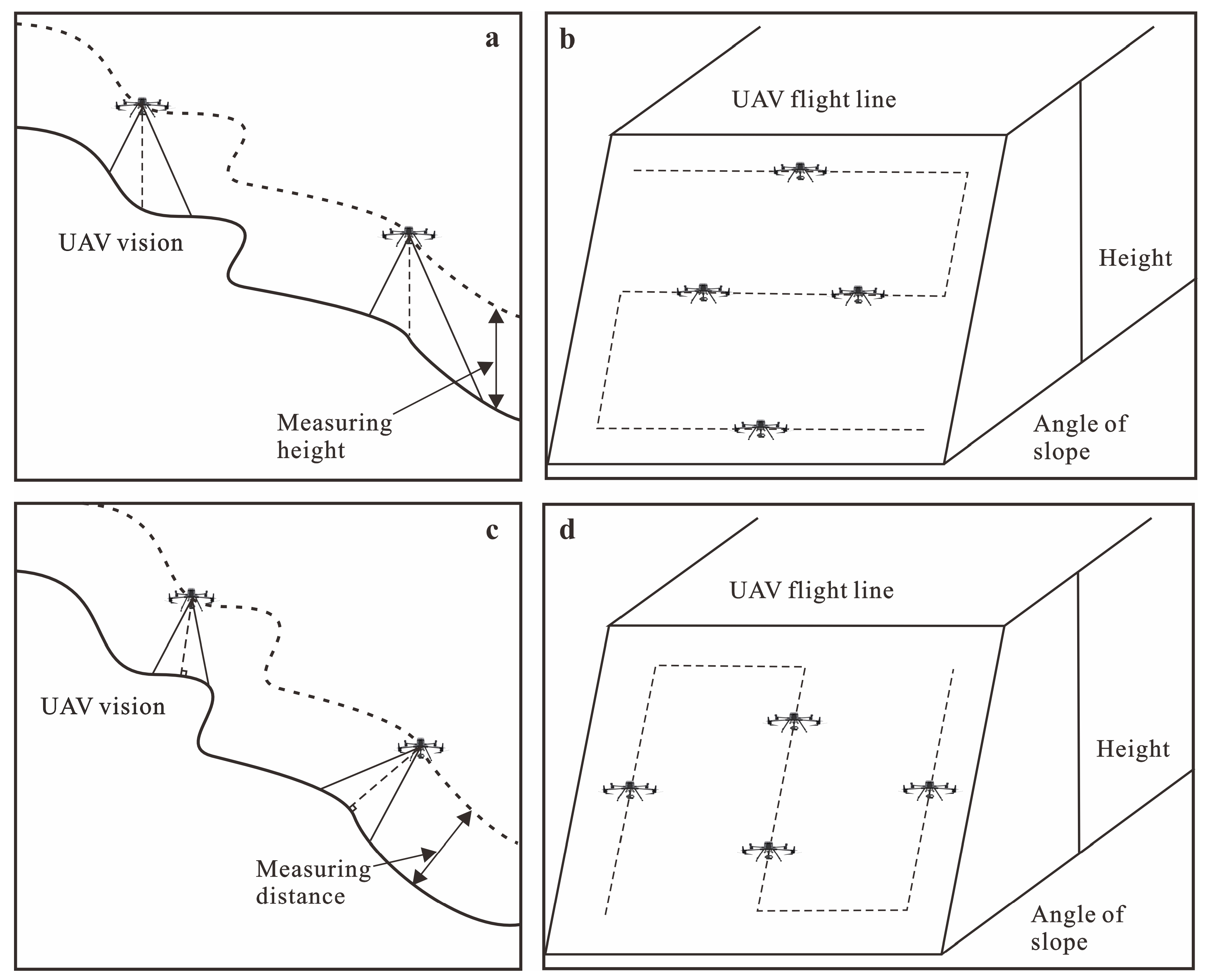
Traditional photogrammetric data struggled to meet the requirements of geological hazard investigations due to the influence of shadow and occlusion. In contrast to conventional five-eye aerial surveys [35], this aerial photography includes TFP and PSSP (Figure 2).

The TFP refers to shooting in the direction of gravity at the same altitude during horizontal flight, and the PSSP refers to shooting at an inclined angle at different altitudes. Combining these two aerial photogrammetry methods can result in more comprehensive measurement results. Specifically, the TFP can provide precise micro-terrain coordinate information, and the PSSP can provide more realistic spatial and texture information, better expressing the complex morphology of the ground. Additionally, the PSSP can capture images on vertical surfaces that are difficult to shoot, such as locations that the orthophoto of dangerous rock mass on the slope cannot cover, and is helpful for the 3D modelling of steep rock slopes. The PSSP takes aerial photography up and down at different altitudes, while the TFP takes the aerial photography at the same elevation. It is also for this reason that the process of slope-changing flight is more time-consuming and power-consuming. In the context of close-range photogrammetry, we observe the side of the rough 3D model while using route-planning software to avoid the interruptions to aerial photography caused by UAV collision.

In this study, we used a DJI M300 RTK UAV (Shenzhen, China) with a DJI Zenmuse P1 lens with 45 million pixels for fusion flight. The TFP route-planning of the left bank slope of the dam was based on a 90 m resolution elevation model (DEM) in Google Earth. A relative flight height of 160 m, a lateral overlap rate of 70%, a longitudinal overlap rate of 80%, and a lens direction perpendicular to the horizontal plane were set. The PSSP route-planning of the area was based on the digital surface model (DSM), obtained through TFP, with a decimeter resolution. A camera tilt compensation of 45°, a lateral overlap rate of 70%, and a longitudinal overlap rate of 80% were set.

2.2. Acquisition of Joint Surface Attitude

2.2.1. Multi-Point Fitting Method

Identifying the rock’s structural plane is a crucial research topic in the rock mechanic field. Although rock structural planes may have undulating characteristics to a certain extent, they can use a plane to approximate. When dealing with geometrically shaped structural planes, one effective method is to extract feature points from 3D models for fitting. Each plane corresponds to an equation, which can obtain the attitude of the structural planes, thereby achieving the rapid and accurate acquisition of high and steep slope rock structural plane attitude.

The exposed structural plane is often unflattening. However, when using fewer feature points to calculate the structural plane attitude, due to the different positions of the selected feature points, there may be some differences in the calculation results, which affects the calculation accuracy. In order to solve this problem, this study uses the multi-point fitting method for plane fitting. Unlike the fewer feature points used to calculate the structural plane attitude method, the multi-point fitting method is suitable for selecting multiple representative points on the rock structural plane in the 3D model image. The coordinate data that are derived can be used for the accurate calculation of the structural plane attitude. The advantage of this method is that it can better calculate the overall structural plane attitude and reduce the errors caused by improper local point selection.

In the 3D model, representative and less undulating joint surfaces have circled on the rock structure plane, and their 3D coordinates are derived. The calculation principle is shown in Figure 3.

Assume that the equation of the fitting plane is as follows:

$$Z=AX+BY+C$$

(1)

where $A$, $B$, and $C$ are the parameters of the plane equation ($A$ and $B$ cannot be 0 at the same time, and the normal vector of the structural surface is $\overrightarrow{n}=\left\{A,B,1\right\}$).

The calculation equation can be obtained based on the least-squares method [20]:

$$\left[\begin{array}{c}A\\ B\\ C\end{array}\right]={\left[\begin{array}{ccc}{X}_1& Y_1& 1\\ X_2& Y_2& 1\\ ⋮& ⋮& ⋮\\ X_n& Y_n& 1\end{array}\right]}^{-1}\left[\begin{array}{c}{Z}_1\\ Z_2\\ ⋮\\ Z_n\end{array}\right]$$

(2)

Through the use of this formula, one can obtain the values of $A$, $B$, and $C$. Subsequently, using the correspondence between the structural plane attitude and the parameters of the plane equation, one can quantitatively calculate dip angle $\alpha$ and dip direction $\beta$:

$$\alpha =\left|\mathit{arctan}\left(\sqrt{{\mathrm{A}}^2+{\mathrm{B}}^2}\right)\right|$$

(3)

$${\beta }_0=\mathit{arctan}\frac{B}{A}$$

(4)

According to the different parameter values, the calculated value and the true value have the following relationship:

$$\{\begin{array}{l}\begin{array}{l}A<0\{\begin{array}{l}B\le 0,\beta ={\beta }_0\hfill \\ B>0,\beta ={\beta }_0+2\pi \hfill \end{array}\\ A>0,\beta ={\beta }_0+\pi \end{array}\hfill \end{array}$$

(5)

2.2.2. Joint Surface Attitude Semi-Automatic Geoprocessing Tool (AST) Based on Python

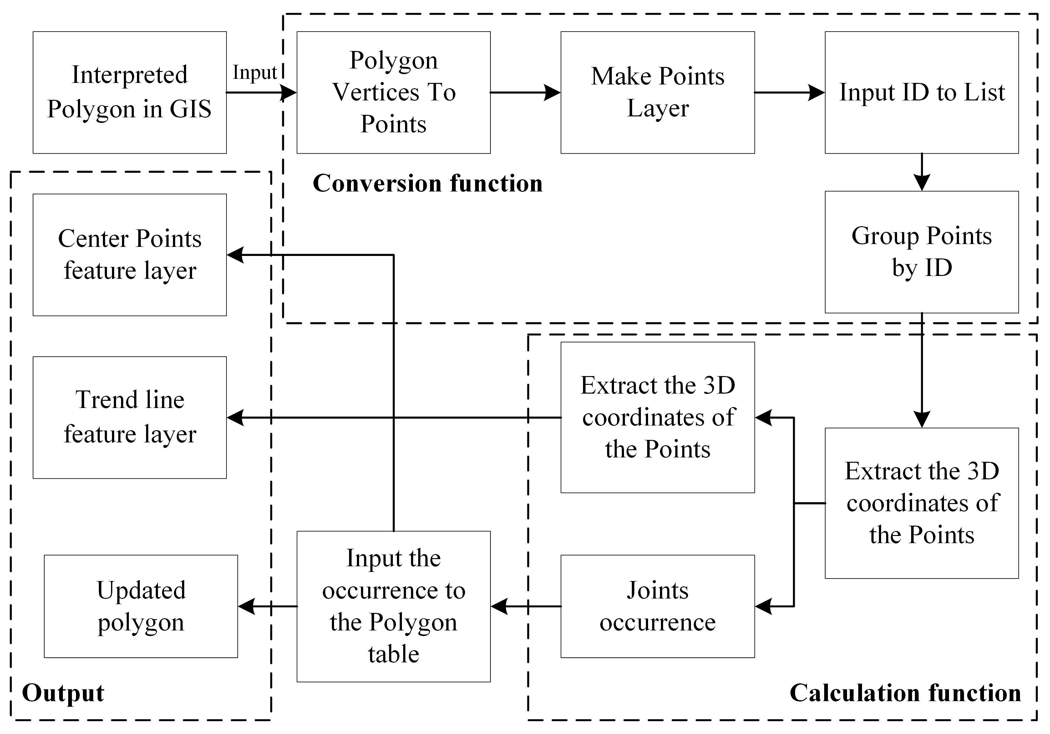
The least-squares method of plane multi-point fitting can be time-consuming and prone to errors. To overcome these limitations and enhance the efficiency of calculations and statistical analysis, we developed a geoprocessing tool for ArcGIS Pro 3.0, using the Arcpy module. The AST processing flow is shown in Figure 4.

The geoprocessing tool consists of five defined functions, including the execution function, conversion function, calculation function, statistics function, and visualization function. Only the execution function’s main body is located in the main program, which includes the interface with the ArcGIS Pro 3.0 and the call to the conversion function. This interface enables the input of feature layers and the output of visualized features. The transformation function first extracts and marks the endpoints of the same polygon. Then, the function using the structured query language (SQL) query statement to screen the point features with the same label for the subsequent calculation of the joint surface attitude. The selected, separated feature layers are deleted after calculation. The statistics and visualization functions are called at the end of this function.

The calculation function uses the cursor to traverse the 3D coordinates of all feature layers and substitutes them into the formula to calculate the corresponding joint surface attitude. When processing coordinate information, x, y, and z correspond to latitude, longitude, and absolute elevation. Selecting incorrect longitude and latitude information will result in errors in the dip direction. The calculated results are written into the corresponding lists in turn for the later statistical function. At this stage, the calculation results are output to two decimal places to meet the engineering requirements. The role of the statistical function is to write the calculated results into the polygon attribute table. First, the list is passed through the add field function to set the dip direction and dip angle property of the list as an integer through the list, whose attribute is added as a string to prepare for visualization. Afterward, the corresponding information is written through the cursor to complete the information statistics and organization.

The visualization functions offer two expressions involving the strike lines and the center points of the joint surface. In the 3D model, the strike line is horizontal, and verifying whether the strike line penetrates the model can eliminate erroneously interpreted data. The length of the trend line displayed on the 2D map positively correlates with the extent of the joint surface, and one can select the appropriate coefficient according to the different application scenarios. To obtain the surface center point, one should use Symbology within ArcGIS Pro 3.0, which can convert the surface center point into an arrow. One can achieve this effect in the figure through additional settings. The visualization results are shown in Figure 5.

2.3. The Verification Methods of TFP and PSSP Fusion Flight and AST

When verifying the effect of the fusion flight effect, first, we compare the amount of image data and the acquisition efficiency. Then, we compare the quality of the images, but image quality is difficult to quantify, so we perform a visual evaluation of typical areas. We compare our method with the commonly used five-eye TFP and single-lens TFP. The lens used in the five-eye imitation ground flight is ShareUAV PSDK102S1161X (Shenzhen, China), with a resolution of 24 million pixels. Because its resolution is different from the 45 million pixels of Zenmuse P1, mentioned in Section 2.1, in order to ensure that the models have a similar resolution, we adjusted the five-eye ground-imitation flight height to 100 m. Other parameters are entirely consistent with those of simulated ground flight, such as heading overlap rate and lens pose.

The verification of AST is mainly compared with manual results’ verification and coordinate geometry (COGO) [36,37] verification. Because the study area makes it challenging to conduct a comprehensive verification of the results, we only verified the results of some areas with slower slope toes. The method of artificial verification is used to effectively measure the attitude of the geological compass on the same joint surface more than three times. After screening out the erroneous information, the average value is compared with the results of the processing tool, and the difference between the results is less than 5°, which is accurate. In order to verify all the occurrence information, we use COGO in the ArcGIS tool to extract the trend line information in batches. Then, we calculate the tendency of the AST and the trend difference extracted by the COGO tool to verify the effect of the processing tool. The absolute value of the difference is about 90° or 270° (±5°), and it can be proven accurate by manually verifying that the direction is correct.

After verifying AST, we also apply it to the 3D models generated by different flight methods for further model quality assessment. The specific method is to use AST to apply the same position to different UAV data acquisition models, and the flight effect can be evaluated by comparing the number of valuable results.

2.4. The Principles of Stereographic Projection and Kinematic Analysis

Slope stability analysis is a significant part of geotechnical engineering [38], which involves aspects such as slope engineering design, construction, and monitoring. There are various methods of slope stability analysis, among which kinematic analysis (also known as geometric analysis) is a simple and effective method. This mainly judges whether rock blocks may slide or be upset, as well as the likelihood of other instability phenomena occurring, based on the geometric relationship between the structural plane and the slope direction in the slope. The kinematic analysis does not require consideration of the forces and stresses acting on the rock blocks. Only parameters such as the orientation, dip angle, and spacing of the structural plane and slope surface should be measured and estimated, and the a stereo-net or stereographic projection can be used to draw the great circles corresponding to each structural plane and slope surface and depict the friction circle and the sliding envelope line to judge whether the rock blocks may become unstable.

One can determine the spatial relationships between each set of structural planes and the slope surface through stereographic projection. Assuming that the influence of straining and other forces between the interior of the rock mass is not considered, only the effect of sliding resistance and the downslide strength of the rock mass are considered. In geotechnical engineering, when the dip angle of the structural planes is opposite to the slope, the slope is relatively stable; when the dip angle of the structural surface is the same as the slope, if the dip angle is greater than the slope, it is relatively stable. Otherwise, it is more likely to lose stability.

Kinematic analysis was first proposed by Markland (1972) and further developed by Hocking (1976) [39,40]. This method has the following advantages: planar sliding, wedge sliding, flexural toppling, and direct toppling based on the geometric properties of structural planes. It can quickly evaluate the slope stability without requiring complex calculations. Researchers can apply it to various slopes, such as natural slopes, excavation slopes, and embankment slopes. Additionally, it can provide a reference for further mechanical analysis.

Table 1. A simple comparison among slope stability analysis methods.

Methods	Preparation Work	Advantages and Limitations
Kinematic Analysis	Joints and slope attitude, friction angle and lateral limit.	Advantages: The failure mode can be accurately determined according to the geometric properties of the structural plane. It can be applied to various types of slopes. The data that are needed to prepare this are easy to obtain. Limitations: Only the set relationship of the slope joint surface is considered, and the mechanical relationship and geological conditions are not considered.
The Limit Equilibrium Methods	The attitude and location of weak surface, geological and structural conditions of the slope, safety factor, friction angle, cohesion of rock mass, etc.	Advantages: The calculation is simple and suitable for slopes prone to gravity mass movements. Limitations: Only the static equation is satisfied, but the compatibility of rock strain and displacement is not considered. The judgment of the location of the weak surface requires some experience.
Empirical Methods	Uses different data for different methods. For RMR, it is necessary to take rock samples to obtain the complete length.	Advantages: For cases with similar conditions, the analysis results of this method are highly reliable. Limitations: Relevant data often need to be obtained through indoor or in situ experiments, which take a long time. This method is not universal.
Numerical Methods	Geological and structural conditions of the slope, suitable mathematical model, and boundary conditions.	Advantages: The free application of load and setting boundary conditions can simulate a more complex slope instability process, and the cost is low. Limitations: The simulation results are abstract and random, the credibility is low, and the accuracy is different.

shows a comparison between these slope stability analysis methods. We can see that the kinematic method has the advantages of requiring less prior knowledge, allowing for easy access, and having a simple mode compared with other methods, consistent with the requirements of preliminary stability analysis.

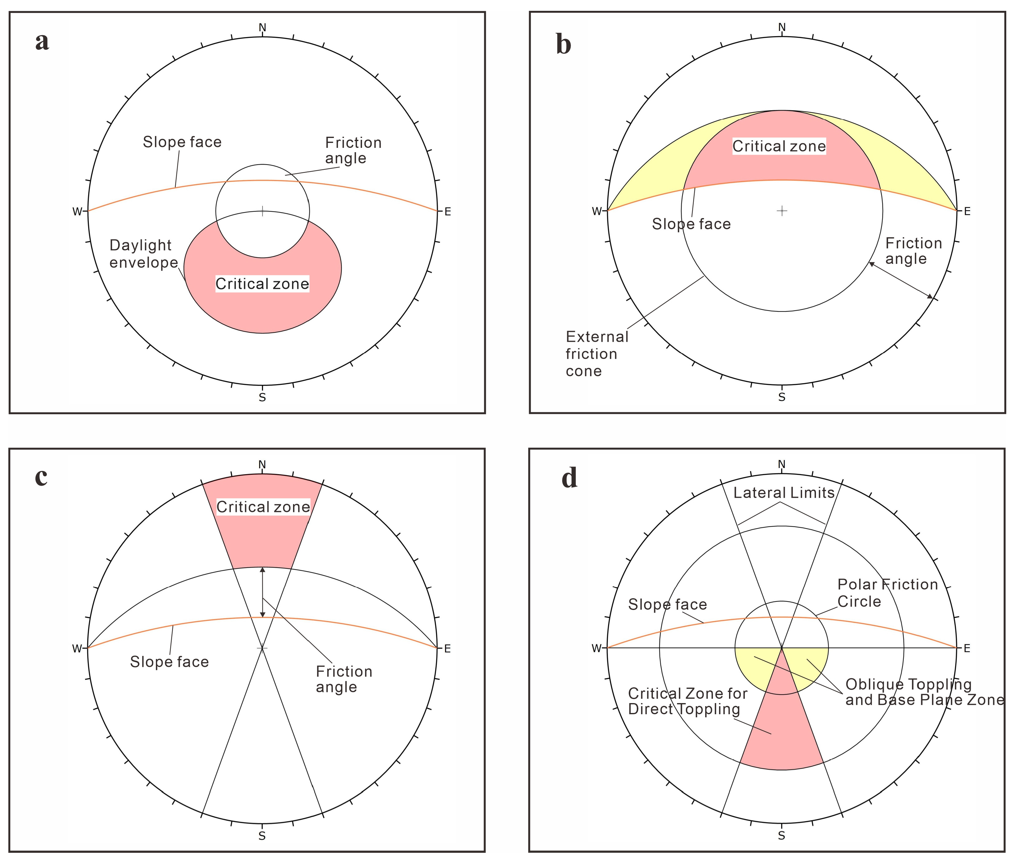
By considering the formation conditions of different failure modes of slopes, a kinematic analysis can be carried out using stereographic projection to determine the failure mode of slopes. This study uses the lower-hemisphere projection, with “pole” referring to the stereographic projection point of the normal vector of the structural plane. “Intersection” is defined as the intersection between joint surface attitude projection arcs. The daylight envelope is one of the boundary conditions for planar sliding, defined as the set of endpoints on one side of a line segment with a length of 90°, where the line segment passes through the center of the projection circle, and the set of endpoints on the other side represents the projection arc of the slope surface attitude. The friction circle defines the limitation of friction stability in the projection diagram. When the poles serve as the failure condition, the polar friction circle is a circle whose center is the same as that of the projection circle and whose radius is the friction angle. When considering the intersections as the failure condition, the plane friction circle center is the same as the projection circle, and the radius is 90° minus the friction angle.

Planar sliding failure (Figure 6a) occurs along the structural plane. The necessary conditions for this failure to occur are that the dip angle of the structural plane must be smaller than its internal friction angle, and the structural plane cannot be steeper than the slope angle. The stereographic projection shows the relationship between the structural planes and the slope. Figure 7a draws a circle representing the slope surface attitude projection, a daylight envelope, and a polar friction circle. The critical zone of planar sliding is the closed region, enclosed by the daylight envelope and the polar friction circle. If the pole point representing the structural plane attitude falls within this region, it means that planar sliding may occur along the structural plane.

When two structural planes meet and form a wedge that can slide along their intersection line, wedge sliding occurs (Figure 6b). Therefore, the dip angle of the intersection line must be steeper than the friction angle of the structural planes. However, the intersection line cannot have a larger angle than the slope angle. At the same time, the trend of the intersection line must be like that of the slope. Stereographic projection is used in kinematic analysis to show the relationship between the structural planes and slope. In Figure 7b, the under-arc represents the projection of the slope surface attitude, and the small circle is the plane friction circle with a radius of 90°-φ. φ is the internal friction angle. The critical zone of wedge sliding is enclosed by the arc and circle. When analyzing the risk of wedge sliding failure, there is no need to worry about lateral confinement because another plane on the side allows for the wedge to move freely for any distance. The effect of this plane is like the sliding or releasing plane of the wedge body.

Flexural toppling failure (Figure 6c) occurs along structural planes. Flexural toppling failure must satisfy the following conditions: (1) the dip angle of the structural plane is steeper than the friction angle; (2) the direction of the structural plane intersects the direction of the slope at a few angles (intersection angle less than 30°). The above conditions form the basis for kinematic analysis. In the stereographic projection, a slope surface attitude projection arc is drawn. Then, the same direction of the slope as the dip direction and slope angle minus the friction angle are used as the dip angle to make another projection arc. Finally, boundary restrictions are drawn according to the direction of the intersection angle. The shaded area in Figure 7c is the toppling failure zone. When the pole of the structural plane falls into this area, flexural toppling failure will occur.

Direct toppling failure occurs along structural planes (Figure 6d). The key elements of direct toppling failure are: (1) two joint sets intersect, causing the intersection line to enter the slope and form discrete toppling blocks; (2) the existence of a third joint, set as a releasing or sliding plane that allows for the blocks to topple. The critical zone in Figure 7d is divided into two areas: red and yellow. The red area is the direct toppling failure zone, and the intersections represent the risk of direct toppling blocks forming, while the yellow area represents the risk of oblique toppling blocks forming. The outer limit (large circle) of the red area is represented by a circle, and the distance from the projection circle to this boundary is the difference between 90° and the dip angle. The outer circle restriction (small circle) of the yellow area is the limit of the plane friction cone. As the intersection point approaches the vertical direction, the possibility of toppling in directions beyond the lateral restrictions increases.

Generally, the residual friction angle of most rocks exceeds the basic friction angle. Based on research on the basic friction angles and residual friction angles of structural planes, the basic friction angle is concentrated between 20° and 35° and the residual friction angle is concentrated between 25° and 50° [41]. In practice, observers have noted that planar failure tends to occur only when the dip direction of the plane falls within a specific angle range in the slope dip direction. Based on experience, values of from 20 to 30 degrees are typically used [42]. For safety reasons, when performing a kinematic analysis of structural planes before conducting further experiments, it is necessary to select the most unfavorable situations within the friction angle range of 20°–35°, with a lateral restraint of 20°–30°.

3. Experiment and Results

3.1. Study Area

The study area is located on the left bank of a hydropower station dam site on the Lancang River in Deqin County, Yunnan Province. The dam site is a transverse valley with a symmetrical “V” shaped canyon and terrain elevations below 2500 m. The slope on both sides of the valley is generally between 40 and 70°, with some parts of the slopes being nearly vertical. However, the mountainous terrain on both sides is asymmetric. The mountain on the left bank is high and large, and the lowest gentle tableland elevation is about 2750~2800 m. However, the right bank has a ridge extending toward the river with the lowest smooth-out tableland elevation of 2500 m [43]. The flow of water at the dam site is turbulent, and during the dry season, the water surface elevation of the river is between 2074 and 2080 m. The width of the river surface is generally between 20 and 60 m, and the water depth is usually less than 10 m [44]. The outcropping strata in the hub area are complex, with a complete range of three rock types. The dam site area is mainly composed of basalt, which is hard rock. The main geological phenomena are effloresced, unloading, toppling, collapse deposit, landslide deposit, and fragmented and loose rock mass [45].

Most of the left bank slope in the dam site area comprises steep slopes with outcropping bedrock, mainly basalt, with an area of about 1.142 km². The distribution area of basalt exposed in this section of the river is approximately 400 m along the river. The mountain is thick, and a small plateau can be seen near an elevation of 2750–2800 m. The angle of the slope below the small tableland is generally between 40–60°. The left bank slope in the dam site area is generally S20~30°E, and the area near the dam site is a near-vertical steep slope. Ravines are developed on the steep slope, and scattered blocks and loose debris deposits can be seen in the gullies and gentle slopes [43,46]. After the failure of the dangerous rock mass on the left bank appended, the rock mostly rolled down along several main gullies toward the 214 National Highway or the Lancang River (Figure 8). The lithologic and rock unit data information used for the strata were obtained from exploration reports of the study area.

3.2. The Verification Results of TFP and PSSP Fusion Flight and AST

The TFP and PSSP fusion flight obtained 2335 images in 3 h, the five-eye TFP obtained 7580 images in 1.5 h, and the single TFP obtained 1083 images in 1 h. Because the five-eye TFP changes the row height of the ground-like flight without changing the parameters that influence the working time, such as image overlap rate, its flight time is slightly longer than that of the single TFP.

It can be seen from Figure 9 that Figure 9a has a higher image resolution than the other two, and it achieved a better performance in the steep and rock-blocked positions, which could not be obtained in the orthographic direction. Figure 9b shows some improvements in detail, but there is still a gap between its resolution and that of Figure 9a. The reason for this phenomenon is the unsuitable setting of the relative flight height; the model with a lower relative flight height should demonstrate a better performance in Figure 9b. Figure 9c shows a good performance in the orthographic direction. However, there are serious image cracks and shadows in the positions that cannot be obtained in the orthographic direction, resulting in darker and blurred models.

Next, manual measurements are taken to verify the AST. Because the slope is very high and steep, only the joint surface outcrops near the highway and at the top of the study area are selected for measurement and verification. We measured a total of four rock outcrops and compared the AST (

Table 2. Manual verification results and AST results comparison table.

Joint ID	Average Value of Manual Measurement	AST Value	Dip Angle Error	Tendency Error
J1	115°∠79°	117°∠82°	3°	2°
J58	52°∠64°	50°∠65°	1°	2°
J116	46°∠84°	46°∠85°	0°	1°
J117	36°∠79°	37°∠77°	2°	1°

). Although we only carried out a small amount of verification for the study area. However, in other slopes where it is easier to measure the joint surface in situ, we have verified it. The results are the same as the study area. From this, it can also be verified that AST can make correct trend judgments and dip angle calculations.

In order to conduct a more comprehensive assessment of the study area, we used the COGO tool in ArcGIS for verification. For the specific method, please refer to Section 2.3 of this paper. Our verification results show that 3 out of 185 samples showed an incorrect tendency in the models obtained by the TFP and PSSP fusion flights. The reason for this is that these surfaces are very steep and contain rock occlusion. Although the model is not explicitly reflected in the visual, the model is still cracked, resulting in coordinate interpolation errors. In addition, we applied it to 185 of the same positions in the five-eye TFP. And the results showed that there were eight samples with large deviations, these samples were all caused by a model cracking or missing, which shows that our flight plan is a great help in improving the quality of the model. For the single TFP modelling, because most of its positions were cracked or missing, we did not have to carry out further comparison and verification.

3.3. Fusion of Aerial Photography

The study area exhibits severe deformation phenomena, including gullies, ravines, and rock weathering, with a widespread distribution. Due to the lack of an effective means to obtain UAV photogrammetry of nearly vertical objects (steep rock slopes) [15], the traditional UAV photogrammetry scheme cannot carry out effective 3D modeling to obtain more comprehensive information on the attitude of rock joint surfaces. Therefore, this study designs a multi-level and multi-angle stereo aerial photography scheme, which includes TFP and PSSP. TFP is used to obtain a consistent surface resolution 3D model of the study area, while PSSP is used to enhance the terrain information of escarpments and rugged gorges.

The fusion aerial flight task was carried out with five flights, taking approximately 3 h to obtain 2335 images. The fusion aerial flight task was carried out with five flights, taking approximately 3 h to obtain 2335 images. TFP resulted in the generation of a TFP measurement plan of the study area (Figure 10a), with 1083 images being captured. PSSP was set to generate a close-range photogrammetry plan of high and steep slope areas (Figure 10b), resulting in the capture of 1252 images. Employing the fusion aerial flight mode of TFP and PSSP decreases the time and effort needed to capture vertical and oblique images separately. This approach produces a higher-quality 3D slope model, improves the 3D model’s clarity, and mitigates distortions resulting from images missing. Figure 11 shows the advantages of combining the two routes.

3.4. The Spatial Distribution of the Interpretation of Joint Surface

The 3D slope model accurately depicts the exposed geometry of the joint surfaces through observation. Most structurally stable joint surfaces appear as regular flat surfaces, and were easily identified and interpreted using the 3D model. The 2 cm ground-resolution 3D model was generated using optical remote sensing images obtained by the DJI M300 RTK. A total of 130 exposed surfaces were selected in the 3D model using the empirical discrimination method.

The preparation work of AST only requires the selection of exposed joint surfaces in the GIS environment. It should be noted that point selection should be carried out after the model is fully loaded. Due to the large amount of data in the 3D model, the image will reload when zooming the model to select accurate point coordinates. Other requirements include choosing a flat joint surface with an apparently regular distribution on the side using the create polygon feature tool, and selecting a horizontal and elevation coordinate system in meters for the specific settings. The reason for picking a coordinate system in meters is that using latitude and longitude coordinates for calculation will result in a vertical plane with a dip angle of 90° due to the inconsistencies in the horizontal coordinate system and elevation coordinate system units, which is incorrect. The reason for using the create polygon feature tool is not only the visualization requirements but also to ensure convenience in processing, which can improve the procedure’s efficiency.

Overall, the joint surface outcrops in the rock mass mainly consist of fragmented sections, and their distribution is relatively concentrated. Most joint surfaces dip between 60° and 80°, necessitating that close attention is paid to the potential for toppling failures in the study site. It can be seen from the model that joint surfaces are more distributed and have smaller exposed surfaces on the northwest slope shoulder and the slope surface near the slope shoulder, mostly in the northeast and southwest directions. The number of exposed joint surfaces in this area indicates severe weathering and the potential occurrence of wedge sliding and toppling failure, so special attention should be paid to rockfall protection. Due to the minimal number of joint surfaces and their steep inclination angles on the slope, the likelihood of planar sliding damage can be reduced. Given that the slope toe includes steeply dipping joint surfaces, it is crucial to conduct a detailed investigation of the structural conditions in this area when constructing a hydropower station. Figure 12 shows the interpretation results in ArcGIS Pro 3.0.

3.5. Stereographic Projection Analysis

Figure 13 shows the stereographic projection of the 130 joint surface attitudes. The following joints were recorded as four sets: Joint1 with a dip angle of 75° and a trend of 43°; Joint2 with a dip angle of 78° and a trend of 313°; Joint3 with a dip angle of 76° and a trend of 97°; Joint4 with a dip angle of 78° and a trend of 238°.

The projection arc of Joint1 is nearly orthogonal to the projection arc of the slope surface attitude, and the circular arc of the structural projection contour is located outside the concave surface of the slope projection arc. Since the dip angle is greater than the slope angle, this group may experience oblique toppling. The projection direction of the joint surface attitudes arc of Joint2 is opposite to that of the slope surface attitudes arc (corresponding to the reverse slope). Due to geotechnical engineering, the reverse slope is stable. However, due to the steep dip angle, it is preliminarily judged that Joint2 may experience toppling failure. The projection arc of the Joint3 surface attitude is similar to that of the slope surface (corresponding to the bedding slope). The attitude projection arc is located within the concave area of the slope surface attitude, and there is an angle between its attitude projection arc and the slope surface; therefore, it can cause toppling or wedge sliding. The condition of Joint4 is similar to that of Joint1 but in the opposite direction. Therefore, it is necessary to pay attention to whether wedge bodies are formed by joint surfaces with similar attitudes, which may cause wedge sliding.

From the above analysis, it can be seen that Joint2 of the left bank slope of the dam site is the first dominant structural group and is the main dangerous surface affecting the stability of the rock slope.

3.6. Kinematic Analysis

Based on the results of the stereographic projection, it is possible to analyze the probability of damage in four modes: planar sliding, wedging, flexural toppling, and direct toppling.

In the experimental area, for the analysis of planar sliding, the pole vector was added to the stereographic projection results of joint density (Figure 13), as shown in Figure 14a. The red arc represents the slope with a dip angle of 47° and a dip direction of 148°. The black circle in the center represents the polar friction circle, and the radius represents the rock friction angle. In this analysis, 20° was used, according to the most unfavorable situation. The threshold region for planar sliding is the red circular area near the center, which contains the daylight envelope and the polar friction circle. Any pole falling within this region may cause planar sliding. In this example, no pole fell within this region, so the probability of planar sliding is 0%, indicating that it is unlikely to occur. On the other hand, if any pole falls outside of the polar friction circle, this means that the slope angle is steeper than the friction angle.

Figure 14b shows a projection of the kinematic analysis of the wedge sliding failure mode. Multiple joint surfaces can divide a rock mass into a wedge and cause wedge sliding. The red arc represents the slope with a dip angle of 47° and a dip direction of 148°. In the most unfavorable case, the friction angle of the rocky slope is 20°. This figure represents the friction angle of the rocky slope as a plane friction circle, indicated by a black circle. The crescent-shaped red area in the figure represents the threshold region for wedge sliding, which consists of the slope attitude projection arc and the plane friction circle. Section 2.3 of this paper provides a definition of the plane friction circle, and its radius in this figure is 90° − 20° = 70°. Figure 14b shows all the intersections of the attitude projection arc that fall within the threshold region. Out of 8384 intersection points, only 218 fall within the critical zone, and the remaining points are not plotted. This result indicates that wedge sliding has little effect on the slope, because points falling within the threshold region account for only 2.60% of the total. Considering the position distribution and number of joint surfaces, the probability that wedges are formed and destroyed almost does not exist.

Figure 14c shows a kinematic analysis of the flexural toppling failure mode using pole vectors. The necessary elements of the flexural toppling analysis are the slope face, slip limit surface, and lateral limit, represented by a red arc, black arc, and two black diameter lines. The red arc represents the dip angle of 47° and dip direction of 148°. The black one represents the angle between the slope dip and the friction angle (20° in the worst-case scenario), which is 47° − 20° = 27°. The two black diameter lines are obtained by rotating the 148° direction line 30° (lateral limit) to each side. The red area bounded by the lateral limit line and the black arc of the slip limit defines the threshold zone for the flexural toppling failure of the slope. In Figure 14c, out of 130 poles, 23 poles are within the critical area, indicating a 17.69% probability of flexural toppling. In Joint2, out of 24 poles, 22 poles fall within the critical zone, showing a likelihood of 91.67% for flexural toppling failure in this joint set. These statistical data suggest that further analysis is required to eliminate the risk of flexural toppling in the inclination direction, particularly for Joint2.

Figure 14d shows a kinematic analysis of the direct and oblique toppling failures using pole vectors. The essential elements of the direct and oblique toppling analysis are the slope face, polar friction circle, release plane, and lateral limit, represented by a red arc, a small black circle, a big black circle, and two black diameter lines. The red arc represents the dip angle of 47° and dip direction of 148°. The radius of the small black circle represents the friction angle (30° in this figure, the worst-case scenario). The distance from the large black round to the edge of the projection circle is the dip angle of the slope face, which is 47° in this figure, so the radius of the large black circle is 90° − 47° = 43°. This study rotates the 148° direction line 30° (lateral limit) to each side to obtain the two black diameter lines. The red area bounded by the big black circle and the two black diameter lines represents the threshold zone for the direct toppling failure. The small black circle and the black diameter lines form the boundary of the yellow area. The yellow area represents the threshold zone for oblique toppling. Intersection points within the red space indicate direct toppling, and those within the yellow region represent oblique toppling. The closer the intersection points are to the vertical direction (the center), the higher the probability of failure. Out of 8384 intersection points, 1104 fall within the red area, indicating a possibility of 13.17% for direct toppling, while 2076 points fall within the yellow zone, indicating a probability of 24.76% for oblique toppling. No pole falls within the two zones, meaning there is a low likelihood of direct toppling along the inherently steeply dipping joint surfaces (base plane) on the escarpment.

4. Discussion

The current mainstream UAV flight planning method mainly uses single-TFP or five-eye-TFP photography. This article combines TFP and PSSP, which have the advantages of a small data volume, a high-quality model, and timesaving qualities. However, the local true 3D concave or convex part joint surface model appears cracked, and image loss occurs in DOM. In the future, the slope flight mode can be further optimized for complex terrains. This paper believes that it is possible to perform single-body surround shooting on the detected dangerous rock mass or the exposed part of the rock mass to minimize the impact of the issues mentioned above and improve the precision of the joint surface occurrence data.

There are still many limitations to the preliminary analysis of slope stability using UAV. Primarily, UAV equipment often exhibits the characteristics of fragility and a high cost, particularly in the case of high-resolution optical lenses, which, at times, may surpass the intrinsic value of the UAV itself. Therefore, the professional training of investigators and the formulation of training standards are also important issues that must be solved in the generalization of the survey process. On the one hand, to protect the UAV, UAV manufacturers have limited the maximum relative elevation of the UAV. Thus, for a high and steep slope (where the relative height of the observation point is more than 1500 m), the UAV cannot carry out fine modeling. On the other hand, the use of drones in this paper, due to their capacitance and resolution, makes it impossible to perform a wide range of 3D modeling.

Because the slope investigated in this case is very high and steep, it is difficult to arrange the ground control points (GCPs), and the GCPs are closely related to the coordinate accuracy of the 3D model [47], which will lead to an overall coordinate offset in the 3D model. These offsets will have a vital impact on the results of the kinematic analysis. The general 3D model contains a large amount of data, which leads to the configuration of the equipment having a significant impact on the interpretation speed of the investigators. The existence of vegetation also has a nonnegligible influence on the quality of the model, which will not only lead to a lack of bare surfaces but also increases the difficulty of interpretation. This is a problem that optical lenses cannot solve. Some researchers have solved this problem to a certain extent by using UAVs with light detection and ranging (LiDAR) [48,49,50,51].

Compared with the direct extraction of structural surface information from point cloud data, this article’s method of using GIS 3D interpretation and extraction has better readability, accuracy, visual results, engineering usability, and data format universality, and is easy to apply and view in GIS software. Although the effect of automatically extracting joint surface information in the existing research is not satisfactory, automatic extraction is a vital step to improve the efficiency of the preliminary analysis of slope stability. Using this step, it becomes possible to directly obtain UAV flight to stereographic projection analysis results, leading to a significant improvement in the efficiency of the work. In addition, this method has the potential to lower the threshold for preliminary analyses of rock mass stability, allowing for on-site investigators to approximate the level of professional exploration workers using UAV flight. Moreover, artificial intelligence models, akin to ChatGPT, can generate preliminary stability analysis reports by producing verbal descriptions from obtained images. The successful implementation of the above predictions can significantly enhance the effectiveness of UAVs in diverse applications, including engineering applications, emergency disposal, and UAV inspections.

Stereographic projection still has many limitations, such as not considering the interaction of forces between rock masses and the filling materials in structural surfaces. Kinematic analysis also has some limitations, mainly that it ignores the force factors that cause rock movement, such as gravity, water pressure, and seismic force; ignores the influence of rock strength and deformation characteristics on slope stability; ignores the interaction between structural surfaces on slope stability; and neglects the effect of time on slope stability. For slopes that need a more comprehensive stability analysis, further and more targeted rock mass stability analyses can be carried out based on the preliminary analysis method to determine rock mass stability proposed in this paper. Through a multi-angle and comprehensive stability analysis of more abundant data, a complete set of methods that can be adapted for slope stability analyses in various actual engineering conditions can be formed, so that the workflow becomes systematic and standardized, and the credibility of stability analyses is improved.

5. Conclusions

This article addresses the challenges of determining the rock slope failure mode, gathering statistics on, and analyzing the joint surfaces of steep rock slopes. It proposes a preliminary assessment method for rock mass stability based on the semi-automatic extraction of joint surface attitude using UAV photogrammetry. The multi-step process includes using UAV photogrammetry data to obtain a precise 3D model of the region. The model is refined through GIS interactive extraction to identify joint surface attitudes. After this, the stability analysis utilizes stereographic projection to perform the analysis. The UAV photogrammetry captures images through TFP and PSSP, resulting in a comprehensive and accurate 3D slope model while reducing the number of aerial photos that are required. We developed a method for extracting and interpreting joint surfaces using GIS with 3D visualization. This method accurately marks the position of joint surfaces to acquire their attitude and spatial distribution. The extracted data are displayed using visual and symbolic representations of the structural surface’s shape, scale, orientation, and location. Through GIS, interrelationships are established, and interactive automation can be achieved. The preliminary stability analysis of rock slope employs the stereographic projection, joint spatial statistical analysis, and a kinematic analysis, focusing on the four aspects of planar sliding, wedge sliding, flexural toppling, and direct toppling.

This study experimented on a 1.142 km² rock slope sited on the left bank of a hydropower station in the Lancang River in China. The experimentation yielded the following results and insights: using two types of flight photogrammetry of the DJI M300 RTK for 3 h, 2335 photos were obtained. This study used images to reconstruct a 3D model with a ground resolution of 2 cm. In the slope model, 130 joint surfaces were interpreted. Among the 130 joint surfaces, 79% had dip angles greater than 70°, and they could be divided into four main groups. The dominant group was Joint2 (313°∠78°). Based on further kinematic analysis using the worst-case friction angle and lateral limit, the probability of flexural toppling, direct toppling, and oblique toppling failures was 17.69%, 13.17%, and 24.76%, respectively, while the possibility of planar sliding and wedge sliding was 0 and 2.60%. The Joint2 group had a probability of 91.67% for flexural toppling failure and was, therefore, the focus of further investigation.

Possible future research directions could include: 1. further optimization of the slope flight mode for complex terrains to improve the accuracy and efficiency of data collection; 2. an exploration of single-body surround shooting on detected dangerous rock masses or exposed parts of rock masses to minimize image loss and improve the precision of joint surface occurrence data; 3. an investigation of other UAV technologies and techniques to enhance the spatial data acquisition and modeling process; 4. the application of the developed workflow to other geological and geotechnical engineering projects for slope stability analyses and assessments of the risk of landslides.

The workflow proposed in this paper effectively solves the problem of quickly and effectively judging the stability of a rock slope when prior knowledge is lacking. Next, investigators can use 3D models and DOM to analyze the investigated site from the perspective of geomorphology and verify the preliminary results. The investigators can also use the attitudes and position of the joint surface to establish a new slope model for numerical simulation analysis. The dangerous joint group and the failure mode are helpful in determining the weak position, carrying out a geophysical exploration or rock sampling, and further determining the risky surface of the slope. Overall, this workflow combines UAV 3D photogrammetry and GIS techniques to efficiently acquire, process, and analyze data related to joint surface attitudes and slope stability. It offers a user-friendly and efficient approach to landslide research, providing valuable insights for geological surveys and engineering practices.