Article

Downscale Inversion of Soil Moisture during Vegetation Growth Period in Ebinur Lake Watershed

1
College of Geography and Remote Sensing Science, Xinjiang University, Urumqi 830017, China
2
Xinjiang Key Laboratory of Oasis Ecology, Xinjiang University, Urumqi 830017, China
3
Key Laboratory of Smart City and Environment Modelling of Higher Education Institute, Xinjiang University, Urumqi 830017, China
*
Author to whom correspondence should be addressed.
These authors contributed equally to this work.
Remote Sens. 2024, 16(6), 983; https://doi.org/10.3390/rs16060983
Submission received: 2 January 2024 / Revised: 29 February 2024 / Accepted: 6 March 2024 / Published: 11 March 2024

Abstract

:
Soil moisture content is an important measure of soil health, and high-precision soil moisture trend analysis is essential for understanding regional ecological quality in the context of climate change, flood monitoring, and water cycle processes. However, in the arid regions of Central Asia, where data are severely lacking, obtaining high-spatial-resolution, continuous soil moisture data is difficult due to the scarcity of stations. Moreover, because soil moisture is easily affected by evaporation time, surface morphology, and anthropogenic factors, mature theoretical models or empirical or semiempirical models to measure soil moisture are also lacking. To investigate the distribution and trend of soil moisture in the Ebinur Lake water, in this study, microwave remote sensing and visible remote sensing data were selected as inputs, and the Global Land Data Assimilation System (GLDAS-2.2) data products were downscaled using the GTWR model, which increased the spatial scale from 27,830 m × 27,830 m to 30 m × 30 m. The phenomena involved in the soil moisture change cycle, spatial distribution, temporal variation, and internal randomness distance were analyzed in the study area through wavelet analysis, Theil–Sen trend analysis, the Mann–Kendall (MK) test, and a variogram. This study obtained high-resolution continuous soil moisture data in the arid and data-scarce region in Central Asia, thus broadening the field of multisource remote sensing analysis and providing a theoretical basis for the construction of precision agriculture in northwest China.

1. Introduction

Soil moisture content strongly affects the meso- and large-scale convective systems within a region and impacts relative air humidity and precipitation. In recent years, many researchers have analyzed land watershed changes, soil health status, and air humidity by establishing soil moisture datasets [1]. In this field, selecting accurate and appropriate soil moisture datasets for the geographical characteristics of the study area has a crucial impact on research outcomes. Currently, commonly used soil datasets such as GLDAS and the NASA-USDA Enhanced SMAP Global Soil Moisture Data (SMAP) provide continuously monitored global soil moisture data on a long-term time-series scale [2,3]. However, these long-term soil moisture products often suffer from low spatial resolution and serious spatial heterogeneity, so they do not accurately or sufficiently reflect the characteristics of soil moisture change for studying the arid areas in Central Asia. In practical research, to address this issue, in situ measured data, visible remote sensing, microwave remote sensing, and other data are often combined and then used to produce soil moisture datasets that reflect the actual conditions of specific regions through machine learning or mathematical models, which can then be used for further analysis [4].
In recent years, many scientific methods have been developed to produce high-resolution, accurate, and reliable soil moisture datasets. The method that was widely applied in the early days in the field involved using various geoprocessing models (such as the Soil and Water Assessment Tool (SWAT), Water–Cloud model, etc.) to simulate soil moisture by establishing a database as input for the study area. These methods have long been used for soil moisture applications in data-poor areas. The advantage of these approaches is that they can be used to obtain more precise soil moisture data through simulation. However, they are easily affected by natural factors such as terrain fluctuations and vegetation coverage, making them unsuitable for retrieving soil moisture in areas with complex environmental elements [5]. Another approach involves using Global Navigation Satellite System Interferometry and Reflectometry (GNSS-IR) technology for soil moisture retrieval. With this approach, the interferometric reflection signals from GNSS data receivers installed in the study area over a long period are used. This approach is based on the difference in interferometric reflection signals generated by different soil moisture conditions. By combining these data with actual measured soil moisture, the surface soil moisture in the surrounding area can be estimated within a certain range. The advantage of this method is its ability to generate stable long-term time-series data with high temporal resolution and low error. However, in data-poor areas in Central Asia, stable GNSS data receivers are often lacking, and the effective range obtained using reflection–signal-based methods is limited by the Fresnel reflection zone, preventing signals from being obtained over large areas [6,7].
Another method that has been rapidly developed in recent years is image-based inversion of soil moisture based on satellite remote sensing data, which is performed through mathematical models, statistical principles, or machine learning methods based on the link between reflectance and measured soil moisture. The most important feature of these methods is their operability and ease of access to soil moisture data on a large scale. Shortcomings include limitations owing to spectral signal penetration, so only data at the surface soil (0~10 cm) can be effectively inverted; for deeper locations, obtaining soil moisture data through direct inversion is difficult, so empirical formulas or machine learning algorithms must be used to deduce values [8]. In recent years, with the development of remote sensing fusion technology, the use of multisource remote sensing fusion data, such as visible light and microwave, for soil moisture inversion has gradually become a mainstream method. This method involves the combination of various band indices that highlight the soil moisture characteristics in visible spectral remote sensing data and the backscattering coefficient features of microwave remote sensing data for different soil moisture contents. Compared with methods that only use a single data source, this approach can, to some extent, overcome limitations due to the weak penetration of visible light signals, effectively increasing the accuracy of soil moisture inversion [9].
The fusion of visible-spectrum and microwave remote sensing data for analysis is a hot research topic in the field of geosciences and is developing rapidly. The signal penetration characteristics of microwave remote sensing data can be used to more accurately invert surface soil moisture data. Synthetic aperture radar (SAR) sensors, such as Sentinel-1, have high spatial and temporal resolution, and data processing to provide dense time-series data is easy, so these sensors are now widely used in the inversion of time-series indicators. Using this feature, a surface soil moisture reflection coefficient of 30 m × 30 m can be obtained, and combining this coefficient with high-resolution Sentinel-2 data can produce a high-precision soil moisture dataset [10]. In addition, for natural surface environmental elements at the regional level, methods such as geographic process models cannot accurately reflect the real soil moisture situation through inversion. However, the use of microwave remote sensing-based models can eliminate the influence of vegetation cover and be used to establish a relationship between microwave backscattering coefficients and soil moisture. This feature is valuable for the inversion of soil moisture and can increase the accuracy of the fused dataset, overcoming the impact of vegetation cover on inversion accuracy [11].
Remote sensing fusion-based data production technology has considerably increased the accuracy of soil moisture inversion. In regions with long-term measured data, the scattering coefficients obtained can be compared with measured data to produce a dataset. However, for the arid regions of Central Asia lacking measured data, establishing a relationship between the inversion results and actual soil moisture is impossible given the lack of measured data. Therefore, downscaling the existing low-precision dataset is particularly important [12]. Downscaling methods typically involve the use of mathematical models, machine learning, neural networks, and other methods to interpolate datasets with inadequate spatial resolution or from which the desired features cannot be captured for experimental research purposes. Many scholars have demonstrated the feasibility of downscaling methods in data research. For example, Zhu et al. addressed the issue of the scale-dependent effects of different surface state parameters on the spatial variation pattern of land surface temperature (LST) in existing downscaled LST products. They increased the accuracy of the dataset by introducing the normalized difference vegetation index (NDVI), digital elevation model (DEM), slope, and latitude and longitude as covariates using a multiscale geographically weighted auto regressive (MGWR) model [13]. Abowarda et al. used a random forest model to generate a surface soil moisture dataset with a spatial resolution of 30 m. The independent variables used in the model were precipitation and soil texture, resampled at 30 m; land surface temperature (LST), albedo, and normalized difference vegetation index (NDVI) at 30 m [12]. Peng improved the resolution of the MODIS LST product by considering the non-stationary characteristics of the spatiotemporal distribution of the relationship between land surface temperature and explanatory variables. They achieved this improvement using geographically and temporally weighted regression (GTWR) [14].
In recent years, the arid region of Central Asia has become a research hotspot due to policy preferences and urbanization. However, soil moisture research has been constrained by factors such as the lack of suitable datasets and the difficulty of conducting field measurements. The Ebinur Lake watershed is representative of these areas. To study soil moisture changes during the vegetation growth period (April–October) within the Ebinur Lake watershed, the objective of this study was to produce a high-precision soil moisture dataset and analyze the spatial and temporal trends during April–October in the area. First, the downscaled target dataset was transformed from GLDAS using wavelet analysis to extract frequency–domain period information to confirm that the vegetation growth period (April–October) within the Ebinur Lake watershed had suitable period variation. Second, we used the soil moisture backscatter data generated by the microwave data source Sentinel-1 through water–cloud modeling and the WET, NDBSI, and NDVI datasets generated by visible remote sensing Sentinel-2 data as the independent variable database after covariance and spatial autocorrelation analyses. The GLDAS surface soil moisture data, with a resolution of 27,830 m × 27,830 m, was used as the dependent variable database. Third, a high-resolution 30 m × 30 m soil moisture dataset was produced after inputting the dependent and independent variable datasets into the GTWR model, which was validated for accuracy. Finally, the verified dataset was subjected to trend and variance function analyses to obtain the spatial distribution and spatiotemporal variation of the soil moisture in the study area. Accordingly, in contrast to previous studies, we were able to effectively combine microwave and visible spectral remote sensing products to obtain high spatiotemporal-resolution soil moisture data and conduct spatiotemporal trend analysis. We focused on the following objectives: (1) we used the WCM to adjust the microwave remote sensing backscatter coefficients on bare ground and vegetation in the study area to eliminate interference owing to vegetation in soil moisture inversion and to obtain more accurate backscatter coefficients. (2) To produce a 30 m × 30 m soil moisture dataset in the study area, the adjusted microwave remote sensing backscatter coefficients and visible-light indices WET, NDBSI, and NDVI, which are strongly correlated with soil moisture, were used as input data; the GTWR model was used to increase the spatial resolution of the GLDAS surface soil moisture data; the accuracy was validated using measured soil moisture data. (3) The produced soil moisture dataset was used to analyze the soil moisture during the vegetation growth period in the Ebinur Lake watershed each year, from which we determined the spatial distribution, spatiotemporal change, and random spatial distance characteristics of the soil moisture. Our method is easy to reproduce, and the results were validated as highly reliable. This study provides a template for high-resolution soil moisture inversion methods in data-scarce areas and new ideas for determining the spatiotemporal distribution characteristics of soil moisture at large scales.

2. Materials and Methods

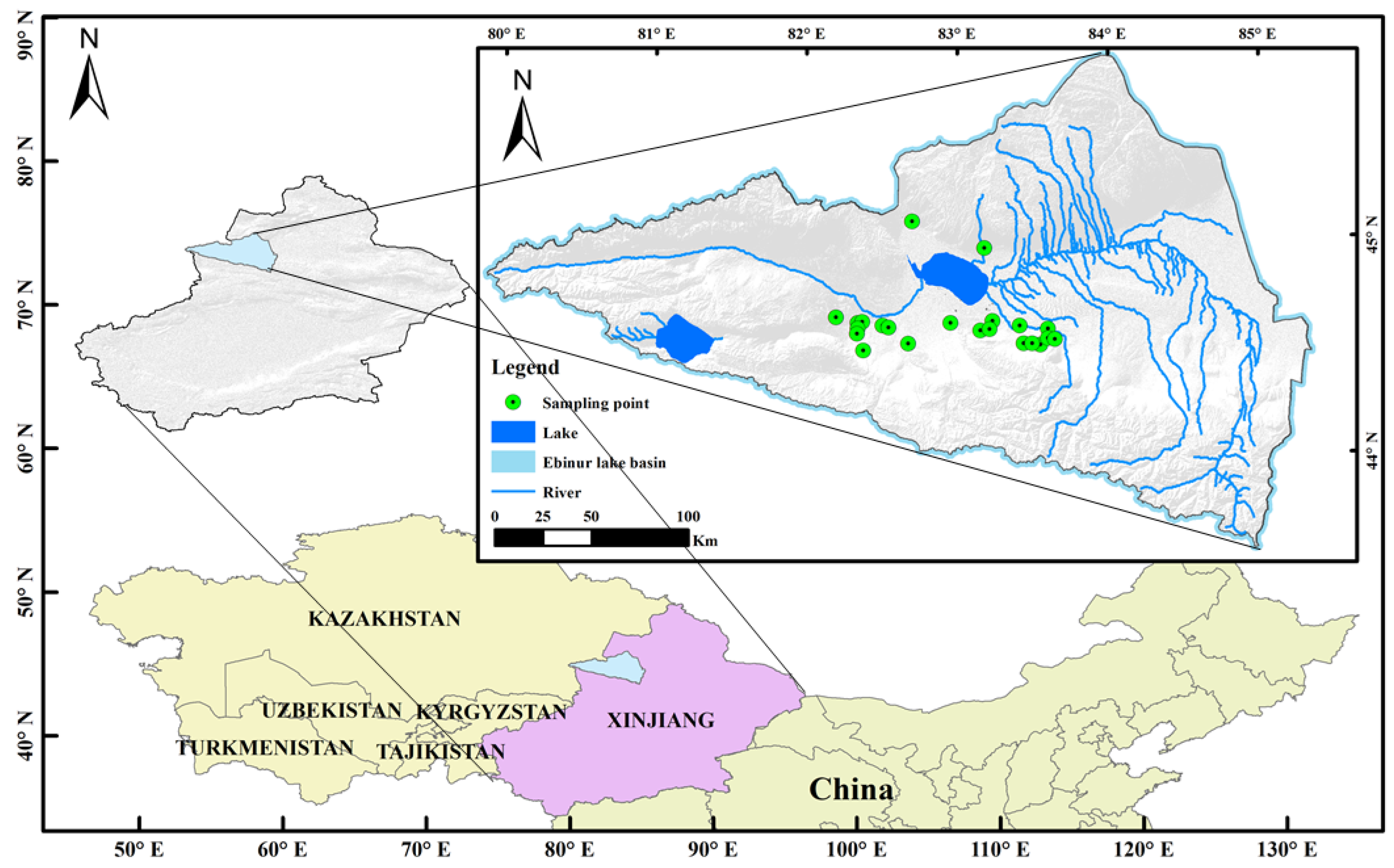
2.1. Study Area Description

Lake Ebinur (Figure 1) is located in northwestern China, and, as the largest brackish water lake in Xinjiang, it plays an important role in agro-industrial water use and ecological stability in the basin. The study area has an arid inland climate with low precipitation (89.80–169.70 mm) due to the lack of humid air, being located far from the ocean, and strong potential evaporation due to long sunshine hours (1569–3421 mm, 6.8 × 10⁸ m3/year) [15]. The main water system in the Ebinur Lake watershed consists of the lake itself and three rivers flowing in from the southwest, northeast, and southeast directions (Jing, Bortala, and Kuitun Rivers, respectively). From a temporal perspective, the recent increase in irrigation and urban water consumption has reduced the inflow into Abbotsford Lake and altered the pattern of soil moisture distribution [16,17].

2.2. Data

In this study, surface reflectance and microwave remote sensing data from the United States Geological Survey (USGS) for the Sentinel series of products, including Sentinel-1 and Sentinel-2, were obtained from the GEE platform. The objects of the downscaled dataset were selected from the NASA GES DISC at NASA Goddard Earth Sciences Data and Information Services Center. The MOD09A dataset was also used as the downscaled visible-light data. Specific information on the data and parameters used in this study are shown in Table 1.

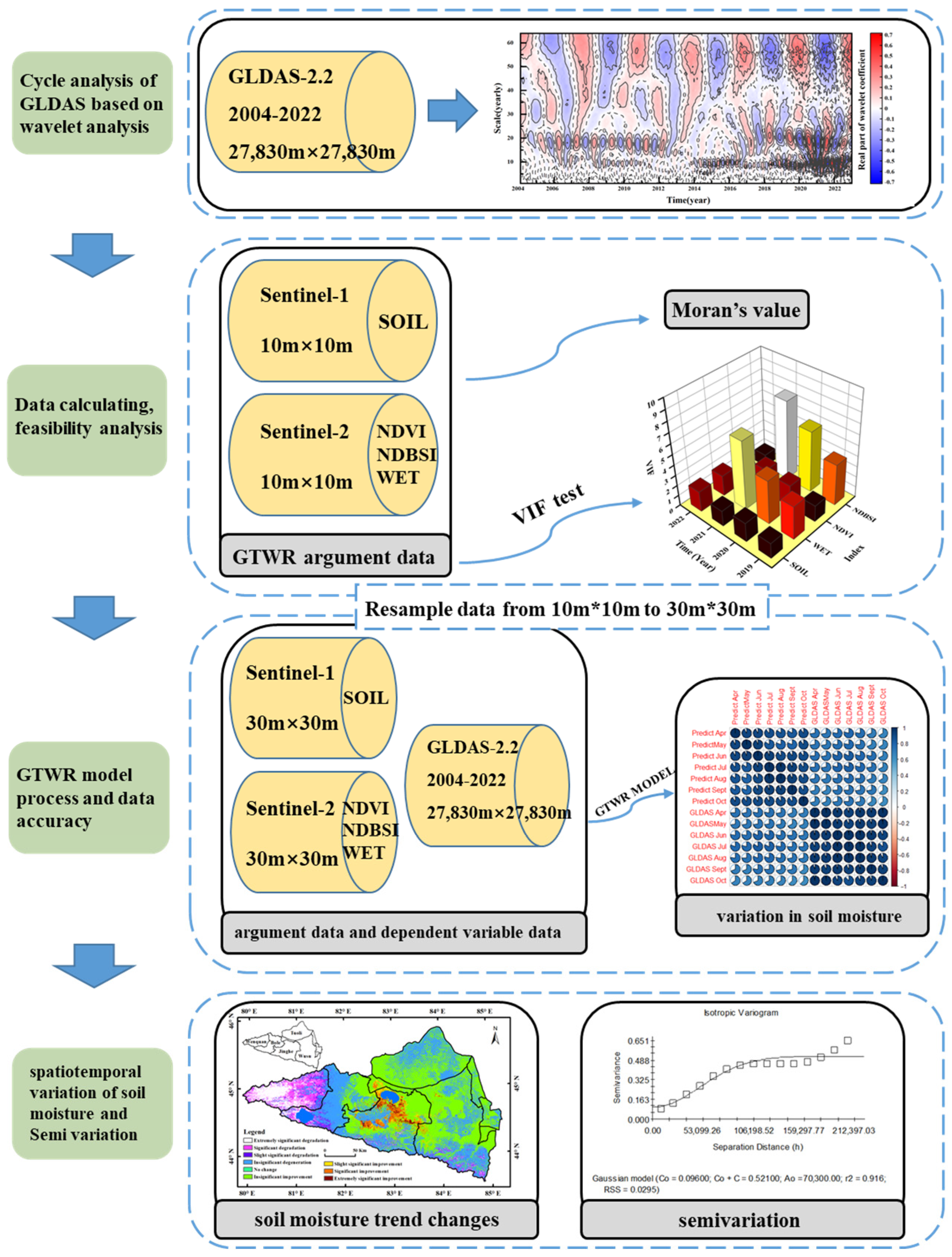
2.3. Modeling of Soil Moisture Downscaling

2.3.1. Water–Cloud Model(WCM)

The water-cloud model is a semiempirical model used for inverting characteristic SAR information that has been widely used in the field of soil moisture inversion in areas covered by vegetation [18]. The model was originally proposed as a supplement to the IEM model for vegetation, specifically describing the microwave scattering mechanism of the land surface in areas with low vegetation coverage, which provides a feasible solution for the inversion of soil moisture and the extraction of backscattering coefficients for nonvegetated areas [19]. The mathematical principle of the model is an assumption that vegetation is a kind of uniformly distributed horizontal cloud on the ground surface. Using this method, the influence of multiple scattering between the vegetation canopy and the ground surface on the inversion of soil moisture can be determined. The complex problem of the range of light scattering from vegetation is abstracted into canopy height and “cloud” density (i.e., vegetation water content) scattering. The overall backscattering from the vegetation cover can be simply divided into two parts: the direct reflection of the vegetation backscatter and the ground backscatter. After removing the double attenuation of crops, this method can be effectively used for the inversion of a large area of low, uniform vegetation distribution. The Ebinur Lake watershed has low and uniform vegetation cover, and vegetation types are mostly low in height, such as cotton fields and pikes, so the area is suitable for the inversion of soil moisture using a water–cloud model. The specific WCM formula is as follows [20]:
σ t o t 0 ( θ ) = σ v e g 0 ( θ ) + γ 2 ( θ ) σ s o i l 0 ( θ )
σ v e g 0 ( θ ) = A cos ( θ ) [ 1 γ 2 ( θ ) ]
γ 2 ( θ ) = exp [ 2 B M v / cos ( θ ) ]
where γ2 (θ) is the vegetation double-layer attenuation factor (transmittance), 0 is the angle of incidence of electromagnetic waves; A and B are the vegetation density parameters, which depend on the type of vegetation and the frequency of incident electromagnetic waves, respectively; Mv is the vegetation water content (kg/m2); θ is the satellite angle of incidence, which was set to 39.46° in this study as the average incidence angle for Sentinel-1A. To determine the vegetation water content, the values of A and B need to be determined first. The water–cloud model is a semiempirical model that Bindlis obtained through a large number of experimental statistical analyses of different surface cover types for different water–cloud model vegetation parameters. The typical vegetation types in our study area were cotton fields, pikes, and other low arid-zone vegetation types, in line with the experimental statistical data for the parameters of winter wheat’s characteristics [11]. As such, A = 0.0018 and B = 0.138 were chosen, and all the parameters obtained by Bindlis after the experiment are shown in Table 2.

2.3.2. Inversion of Vegetation Water Content

The water content in vegetation plays an important role in the inversion of surface soil moisture. Currently, using remote sensing data to invert vegetation water content has become increasingly common. Various methods can be applied for inverting the water content in vegetation, among which the most common one is the use of the normalized difference water index (NDWI) and other normalized visible-light indices. The NDWI is calculated as follows:
N D W I = ( R N I R R S W I R ) / ( R N I R + R S W I R )
where RNIR represents the reflectance of the near-infrared band, and RSWIR represents the reflectance of the shortwave infrared band, which correspond to Sentinel-2’s 8th and 11th bands, respectively. As the study area was dominated by low vegetation in the Golmud River watershed, the vegetation water content was calculated using the empirical relationship between NDWI and VWC (kg/m2), which was established based on experimental data, as proposed by Jackson [21]. The specific formula is as follows:
N D W I : V W C = 1.44 × N D W I 2 + 1.36 × N D W I + 0.34

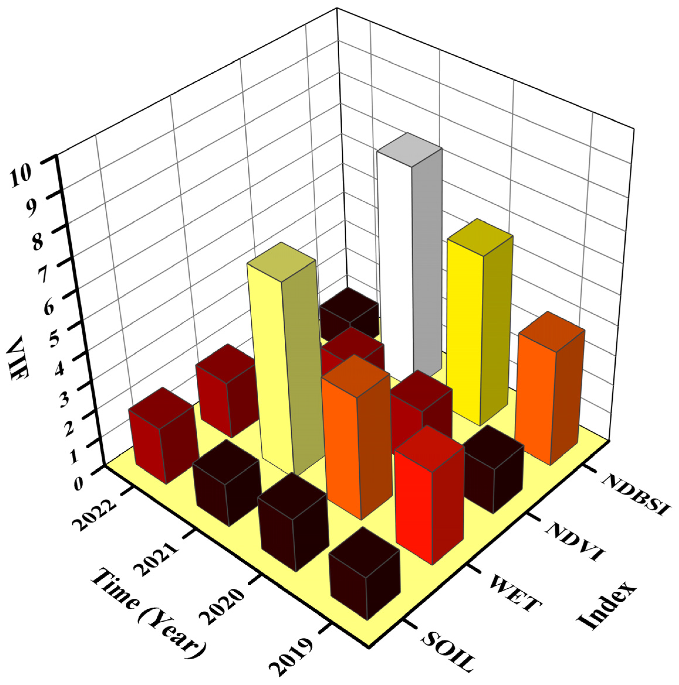
2.3.3. Geographically and Temporally Weighted Regression (GTWR) Model

Before the widespread use of the geographically and temporally weighted regression (GTWR) model, the geographically weighted regression (GWR) model was extensively applied for studying spatial relationship problems. The GTWR has been used to explain the impact of certain independent variables on the dependent variable or predict its future changes by establishing a spatial relationship model [22]. By applying this relationship between variables, coarse-resolution raw data can be enhanced to high-resolution data, while maintaining the spatial distribution characteristics and correlation features in the data. This method effectively enables the long-term monitoring of natural elements in data-deficient areas in Central Asia [23]. The data need to be analyzed for covariance to ensure the feasibility of the model before building the GTWR model. A high degree of correlation among explanatory variables can lead to invalid model estimates under approximate covariance, meaningless significance tests, and reduced prediction accuracy [24]. In this study, the variance inflation factor (VIF) was used to test the explanatory variables for covariance and exclude the variables that caused covariance. The VIF is calculated as follows:
V I F j = 1 1 R j 2
In the formula, VIFj represents the variance inflation factor of the corresponding independent variable, and R2 is the coefficient of determination obtained via regressing independent variable j on the other independent variables. The range of VIF is 0 to ∞. When VIF < 10, no significant collinearity exists. When 10 ≤ VIF < 100, collinearity among the variables is strong. When VIF ≥ 100, collinearity is severe, indicating that the variables cannot be used for modeling purposes [25].
In addition, the spatial autocorrelation between variables must be tested before constructing the geographically weighted regression (GWR) model [24]. In this study, global Moran’s I index, which quantitatively describes the spatial association and distribution characteristics of the samples and determines the degree of spatial correlation of the input variables, was calculated to determine the spatial autocorrelation [26]. The following formula was used to calculate global Moran’s I:
G l o b a l   M o r a n I = n i = 1 n j = 1 n ( x i x ¯ ) ( x j x ¯ ) ( i = 1 n j = 1 n w i j ) j = 1 n x i x ¯ 2
In the formula, n represents the sample size; xi and xj represent the observed values of the attribute at spatial locations i and j, respectively;   x ¯ is the average value of attribute xi; and wij is the spatial weight matrix. We used an adjacency-based weight matrix, where wij was equal to 1 if the ith and jth regions were neighbors, and 0 otherwise.
Finally, the GTWR model was established using the following formula:
y i = β 0 ( μ i , ν i , t i ) + k = 1 p β k ( μ i , ν i , t i ) x i k + ε i
Sample i is represented by yi, which corresponds to the soil moisture concentration. Hi, Vi, and ti denote the longitude, latitude, and time coordinates of sample I, respectively. β 0 ( μ i , ν i , t i ) represents the intercept of a specific position, and β 0 ( μ i , ν i , t i ) denotes the regression parameter of sample i’s kth explanatory variable. Xik is the value of the kth explanatory variable of sample i, and εi is the residual term of the model.

2.3.4. Verification of Model Accuracy

We downscaled the GLDAS surface soil moisture data based on Sentinel-1 and Sentinel-2 data. After obtaining the processed 30 m × 30 m soil moisture dataset, the data were validated using field measurements. The downscaled dataset in this study is expressed in units of kilograms per square meter, whereas the field measurements of soil moisture are expressed as the weight of the soil after drying divided by the weight of the soil before drying [27]. The Pearson correlation coefficients between the downscaled soil moisture dataset and the original GLDAS dataset, as well as the field measurements dataset, were calculated. A strong correlation indicates that the downscaled dataset has similar characteristics to the validation dataset and thus passes the accuracy validation [28]. The formula for the Pearson correlation coefficient is:
r ( X , Y ) = C o v ( X , Y ) V a r [ X ] V a r [ Y ]
where Cov(X,Y) is the covariance of X and Y, Var[X] is the variance of X, and Var[Y] is the variance of Y.

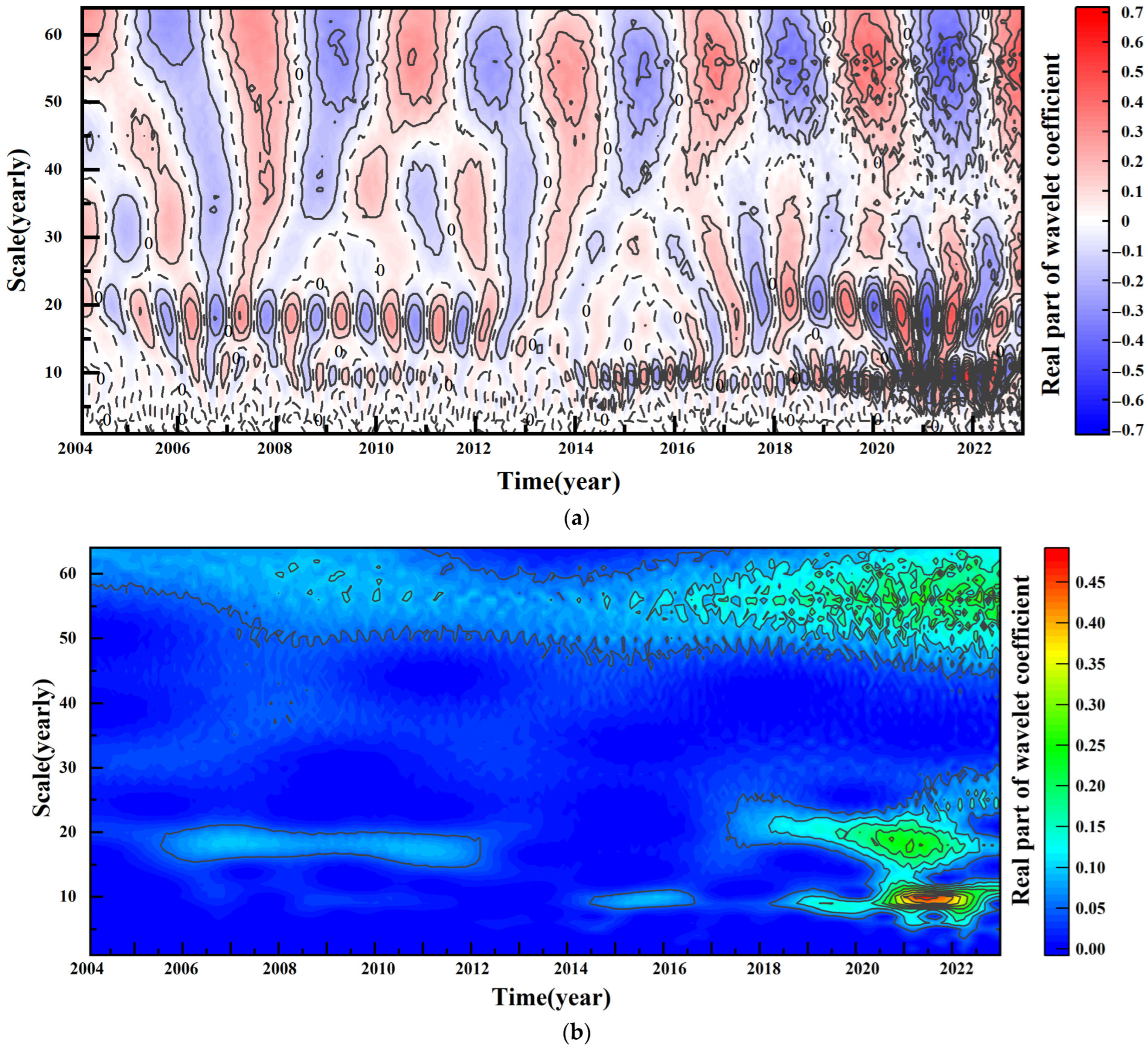
2.4. Morlet Wavelet Analysis

When studying the trend of the changes in geographic factors over time, their features in the frequency domain must often be observed, and they must be analyzed as time-varying periodic signals. Wavelet transform is a classical method used for analyzing periodic signals, which can reflect the changes in a system on different time scales and be used to qualitatively evaluate the future development of these signals [29]. In this study, the monthly soil moisture products were a set of continuous nonstationary time series.The changes of it were affected by unnatural factors that showing irregular fluctuations distributed throughout the year in Ebinur Lake. The application of wavelet analysis enables the identification of hidden cycles within a time series, then enhancing the accuracy in determining the timing and duration of high-frequency soil moisture changes in a given region [14].

2.5. Semi-Variogram

To reveal the various change periods within the time series and qualitatively assess future development, Morlet wavelet analysis can be used to reflect the variation in a system at different time scales and assess the strength and range of spatial correlation in soil moisture within a study area. The variation function, also known as the semi-variogram, is an important concept in geostatistics, used to measure the degree of randomness in soil moisture within a study area. It represents a mathematical model or a composite mathematical model that fits the distribution of the data and reflects the structure of the spatial variability of regionalized variables through its randomness. Hence, the variation function is referred to as a structure function [30]. The semi-variogram can reflect four important geostatistical properties: 1. The internal spatial randomness of the data can be reflected by the nugget effect. This effect measures the variability between points that are a very short distance apart. 2. The strength and range of the internal spatial correlation of the data can be reflected by the variogram. The variogram measures the average dissimilarity between pairs of data points at different distances. 3. The data anisotropy, or directionality, can be determined by examining variogram maps in different directions or angles. This helps identify if the data exhibit different variability patterns across different directions. 4. The spatial continuity of the data can be reflected by the different shapes of the variogram at the origin. Different variogram shapes, such as parabolic, linear, discontinuous, random, and transitional shapes, can indicate different levels of spatial continuity and heterogeneity. These properties help us to understand the spatial characteristics and patterns of the soil moisture within a study area [31]. Semi-variograms are established using the following formula:
γ h = 1 2 E Z x Z x + h 2
where Z x is the regionalized variable, and h is the crement.

2.6. Trend Analysis

2.6.1. Theil–Sen Trend Analysis

Theil–Sen trend analysis is a nonparametric statistical method widely used in regression and time series analyses, mainly for estimating trend lines in datasets [32]. This method is used to estimate the slope of a trend line by calculating slopes between data points. Then, these slopes are aggregated using the median to obtain a final trend estimate. Compared with other approaches, Theil–Sen trend analysis is robust and unaffected by the presence of outliers in the data. It is calculated as:
β = Median ( x j x i j i ) , j > i
where β represents the slope value j; i takes a range of natural numbers, starting from 1.

2.6.2. Mann–Kendall Significance Test

The Mann–Kendall test is a nonparametric test that complements Theil–Sen slope estimation in testing the significance of a time-series trend [33]. When the absolute value of Z is greater than 1.65, 1.96, and 2.58, the trend passes the significance test with a confidence level of 90%, 95%, and 99%, respectively; the test with a confidence level of 95% is generally used. The Sen slope and MK test results were assigned values for reclassification and multiplied to obtain the final significance results, enabling the visualization of the distribution of different change characteristics within the watershed [34,35]. The formula used for this is:
S = i = 1 n 1 j = i + 1 n sgn ( S o i l m o s i t u r e j S o i l m o s i t u r e i )
sgn S o i l m o s i t u r e j S o i l m o s i t u r e i = { 1 , S o i l m o s i t u r e j S o i l m o s i t u r e i > 0 0 , S o i l m o s i t u r e j S o i l m o s i t u r e i = 0 1 , S o i l m o s i t u r e j S o i l m o s i t u r e i < 0
where the number of sequence samples is represented by n, and Soilmoisture and Soilmoisturei are the values for soil moisture in years j and i (where j > i), respectively. When n is greater than 8, S approximately conforms to a normal distribution. By standardizing S, the test statistic Zmk can then be calculated.
The experimental and technological roadmap for this study is shown in Figure 2.

3. Result

3.1. Periodic Results of Wavelet Transform

To determine the temporal variation in the soil water cycle in the Ebinur Lake watershed under a long time series, we conducted a wavelet transform on the GLDAS soil water data from 2004 to 2022, and we obtained the variance trend diagram shown in Figure 3. The figure shows three maximum points distributed on a time scale of 60 months. When the time scales were 56, 18, and 9 months, the corresponding variances were 24, 16, and 16, respectively. This indicated that three main soil water cycles occurred in 2004–2022, and the periodic changes corresponding to the three main cycles could be constructed according to the extracted main cycle information in Figure A1 and Figure A2. In Figure 3b, regular periodic movements can be seen from the corresponding periodic changes during the first main period of 56 months, with a period of 12 months. Similarly, Annex1’s periodic changes during the second main period of 18 months and the third main period of 9 months also show regular periodic movements, and the corresponding periods are both 6 months.
The real part of the wavelet coefficients for the period 2004–2022 was obtained via contour analysis of the real part of the wavelet transform results, as shown in Figure 4. The results of the analysis showed that on the time scales of 56, 18, and 9 months, the corresponding transverse axes crossed the most contour circles, and three main cycles could be extracted, which is consistent with the results obtained from the variance trend plot analysis, as shown in Figure 3. In addition, the contour circles of the first principal cycle are uniformly distributed over the entire time scale. That is, the first main cycle is most accurate for long time series. On the contrary, although the second main cycle has a distribution of isochronous circles in most of the years, a large break exists between 2013 and 2017, which indicates that the second main cycle is not applicable to 2013–2017. Finally, the third main cycle for the time scale of 9 months shows a uniform distribution of iso-circles only after 2014, suggesting no significant cyclical variation within the third main cycle in the time period prior to 2014. Then we get Figure 4,which was obtained after contour analysis of the mode squares in the wavelet transform results. The region where larger values are concentrated in the figure indicates an occurrence of stable periodicity. Combining the results of the analysis of the three main cycles, we found that soil moisture in the study area had stable cyclic variation after 2014, and the scale of the cycle was stable at 6 or 12 months.

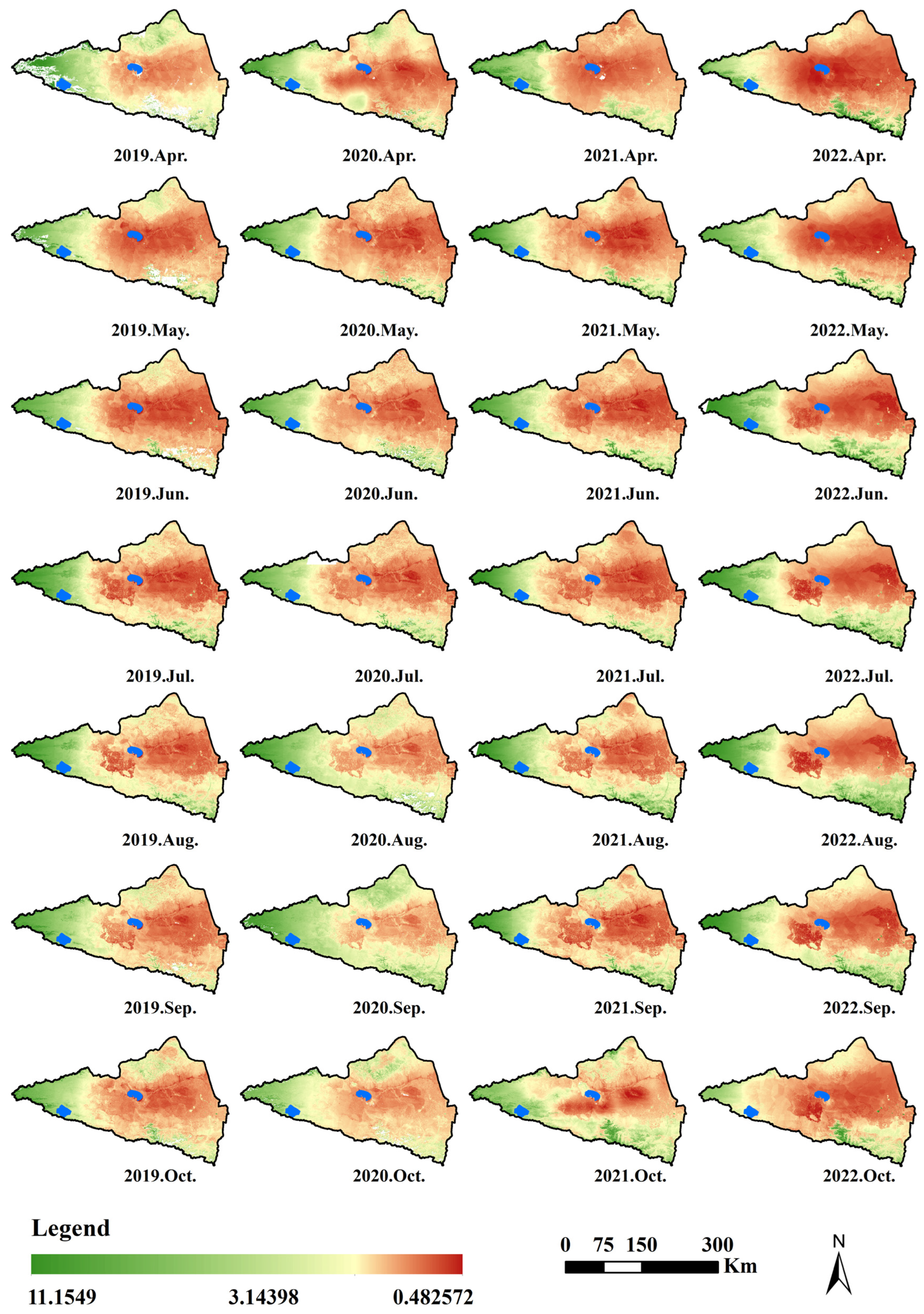
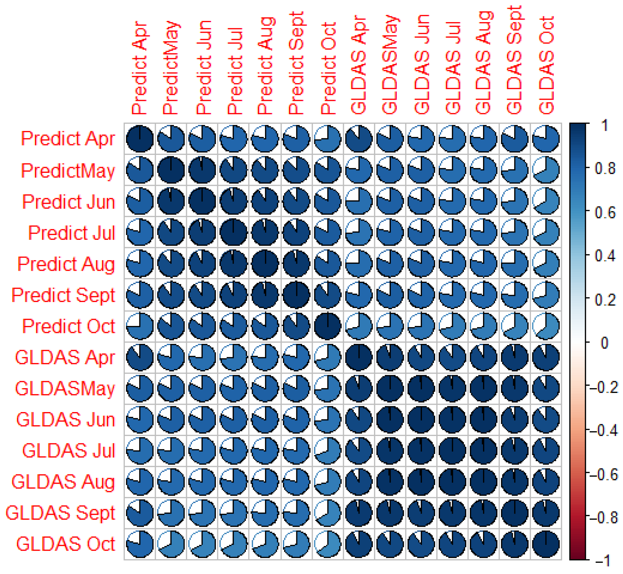
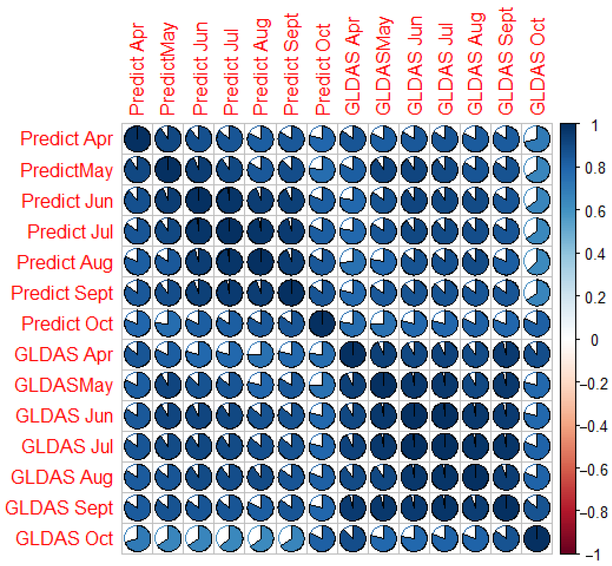
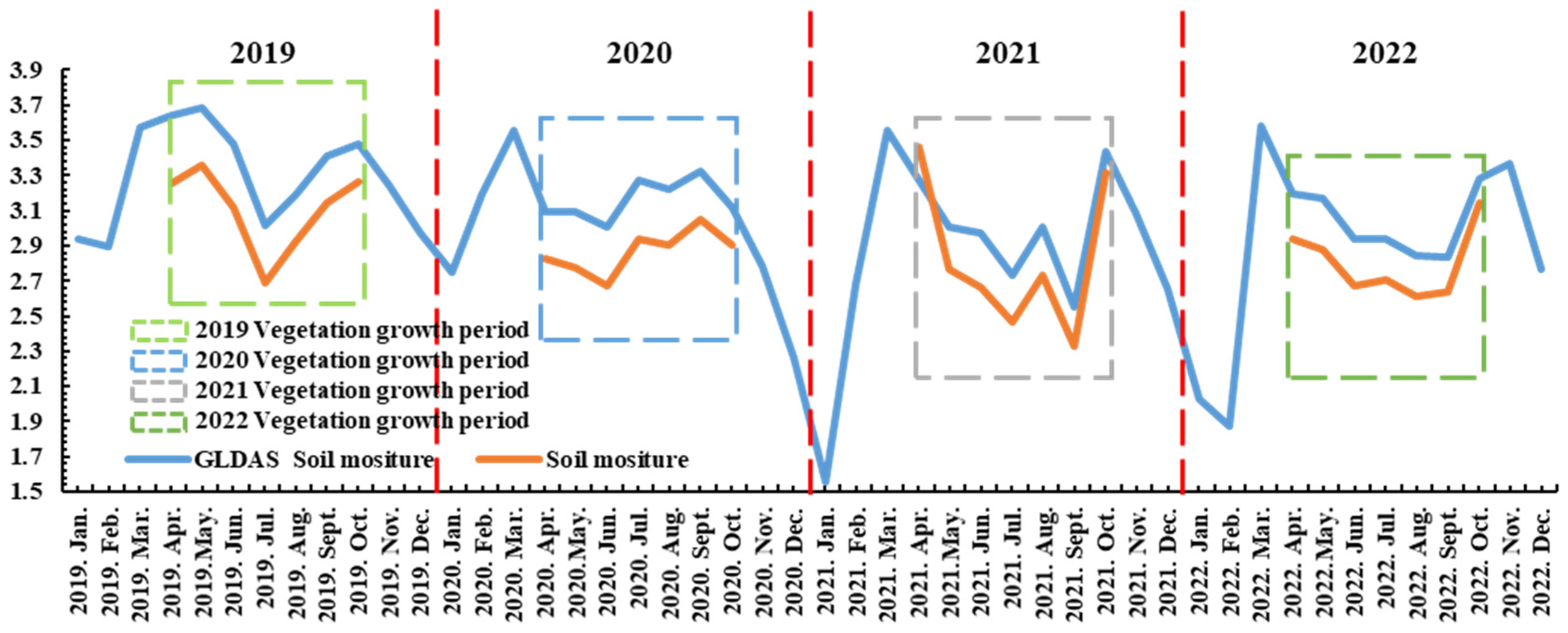
3.2. High-Resolution Soil Moisture Downscaling Results and Accuracy Validation

Before establishing the GTWR model, we analyzed the multicollinearity and spatial clustering of the data using the variance inflation factor and Moran’s index, respectively. The results are shown in Figure 5, Table 3, and Appendix B. Subsequently, the GTWR model was applied to downscale the GLDAS soil moisture data for the years 2019, 2020, 2021, and 2022. The independent variables selected for the model included backscatter data from the water–cloud model, SOIL, WET, NDVI, and NDBSI data. After calculating the VIF values of the independent variables, we found that none of the independent variables in the study area had strong multicollinearity (VIF values were all below 10) during the vegetation growth period, and the maximum VIF appeared in 2021 when the NDBSI index was 7.526628. The WET and NDBSI indices had relatively high VIF values, high covariance with other dependent variables, and did not exceed 10, indicating that these two indices strongly influenced the soil moisture inversion results. Then, a spatial autocorrelation analysis was conducted on the four independent variables: SOIL, WET, NDVI and NDBSI, using GTWR. The results are shown in Table 3 and Appendix C. Table 3 reveals that the Z-value of Moran’s index for all factors in different years was more than 100, and the p-value was zero, which indicates that the four independent variables were strongly autocorrelated in all years and could be analyzed by downscaling soil moisture data using the GTWR model.
The downscaled soil moisture dataset is shown in Figure 6 and Appendix C, and the analysis showed that the downscaled dataset had stable residuals and strong correlation with the original GLDAS data, with notable periodicity. The periodicity obtained from the wavelet transform analysis in the previous section was satisfied. A 30 m × 30 m resolution soil moisture dataset for the vegetation growing period (April–October) in 2019, 2020, 2021, and 2022 was created from the watershed. Then, the data needed to be validated to ensure its scientific value and accuracy.
For accuracy validation, the 30 m × 30 m soil moisture dataset produced using the GTWR model was first correlated with the source GLDAS data to verify that the downscaled data retained similar spatial distribution characteristics as the original data while increasing accuracy. Second, the correlation between the produced dataset and the measured data was verified using Pearson’s correlation coefficient. A total of 900 sampling points were randomly arranged in the study area, and 786 sampling points were obtained after the blank values were eliminated from the GLDAS data. The Pearson coefficient was used to analyze the correlation between the GLDAS data and the predicted values obtained from downscaling for the vegetation growing months in 2019, 2020, 2021 and 2022 (Figure 7a and Appendix D). The analysis revealed that the correlation coefficients between the obtained high-resolution data and the GLDAS data were all more than 65 and passed the 90% significance test, indicating that the downscaled data strongly correlated with the source data. We successfully increased resolution and strengthened the local details while retaining the characteristics of the spatial distribution and temporal change of soil moisture in the original data.

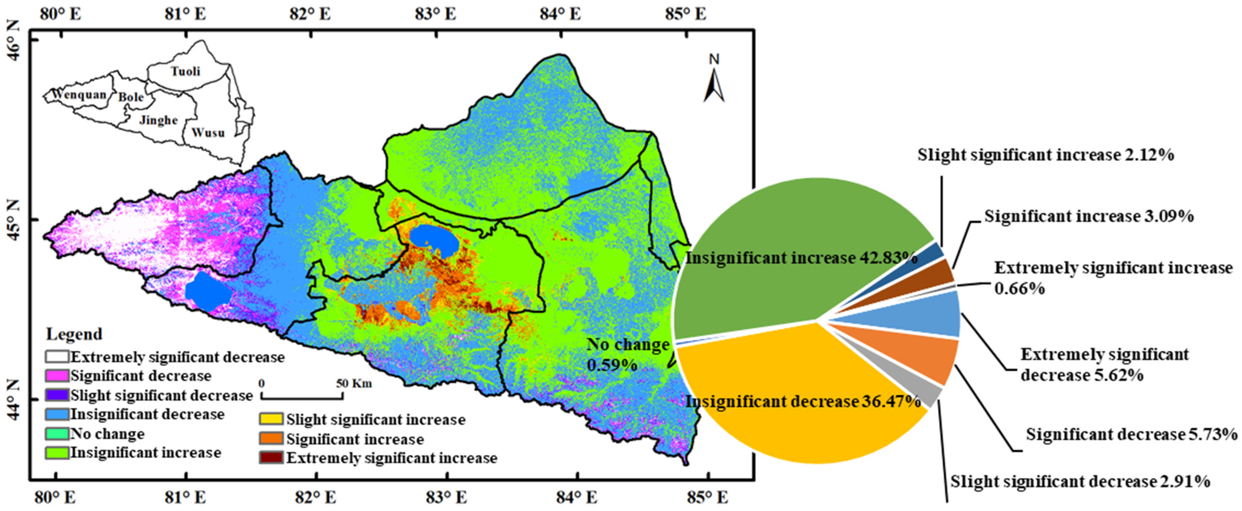
3.3. Trend Analysis of RSEI in the Aral Sea Basin

To verify the reliability of the data regarding the degree of soil moisture change after the analysis of trends data obtained from April to July for the annual average and we test the result for significance to ensure it could reflected the spatial and temporal changes in soil moisture.As shown in Figure 8, eight types of significance test results were obtained in the watershed, at the 99.5%, 99%, 98%, 95%, 90%, 80%, 50%, and failed levels. Figure 8 shows that the overall significance results within the watershed were high in the west and east. The significance was higher in the western region, with most results attaining a significance level of more than 95%. The areas that did not pass the significance test were mainly concentrated in the northern, eastern, and central parts of the watershed. Highly significant types were also distributed in the central part of the study area, close to the wetlands of Ebinur Lake. Overall, we concluded that the SEM-MK trend analysis method is more effective for wetlands or areas with high soil moisture content and could objectively and accurately represent the real situation in the watershed.
After obtaining the proof of significance results, the spatial and temporal variations in soil moisture in the Ebinur Lake watershed were analyzed (Figure 9). First, we found that soil moisture change could be divided into nine categories. Among these, areas where soil moisture did not significantly change only accounted for 0.59% of the total area. This finding indicates that almost all regions underwent different degrees of change in soil moisture, and the entire watershed’s soil moisture was in dynamic equilibrium. The largest area was classified as insignificant increase, which accounted for 42.83% of the total area, spatially covering various locations within the watershed, including Bole in the west, Tuoli in the north, and Jinghe and Wusu in the south. However, these areas were less common around the Lake Ebinur wetland, which is mainly due to the lake serving as a permanent body of water on the surface to maintain the soil moisture balance in the surrounding areas. The next largest area type was categorized as insignificant decrease, which accounted for 36.47%. Areas with insignificantly increasing soil moisture occupied a total of 79.3% of the area of the study area; an extremely significant increase in soil moisture was observed in the study area, mainly in the Wusu area. Increases in soil moisture in the study area were mainly located in the southern part of the Ebinur Lake wetland in Jinghe; this area experienced the largest increase in soil moisture in the watershed, which is related to the expansion of Ebinur Lake during the vegetative growth period. The most significant decrease in soil moisture in the study area occurred near Wenquan on the western side, which is related to natural factors such as higher elevation. Overall, soil moisture in the Ebinur Lake watershed is in a relatively balanced state, with no major ecological changes occurring.

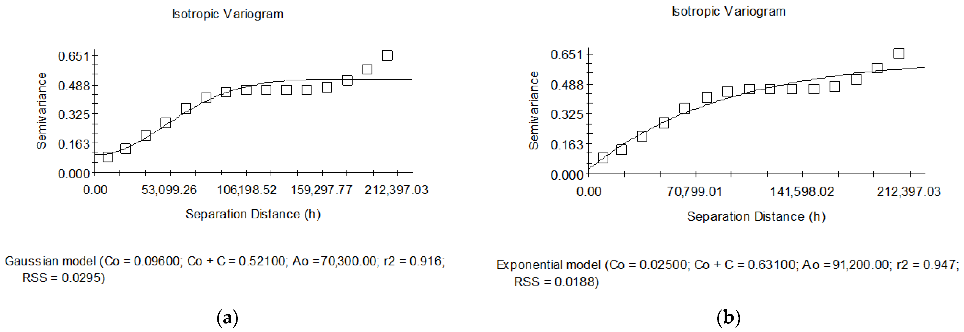
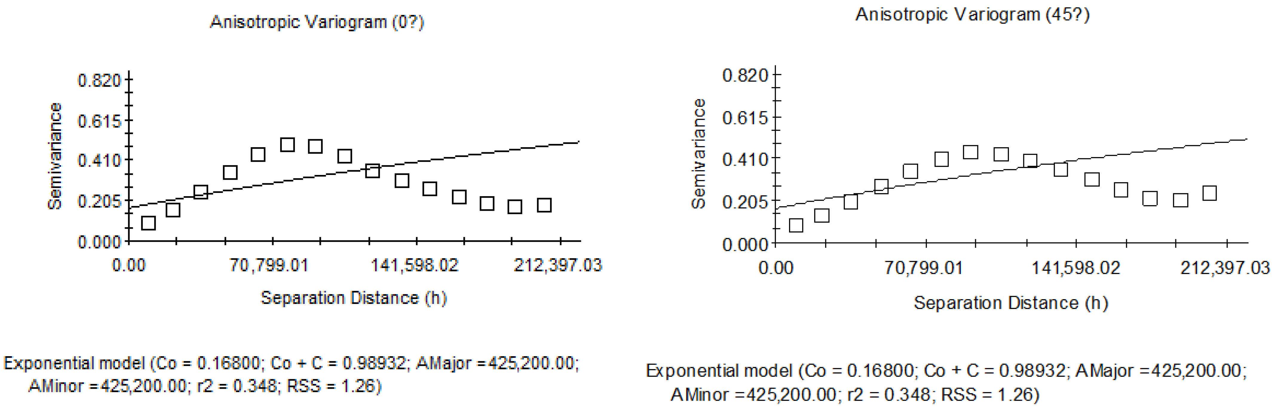
3.4. Semi-Variogram Results

The generation of a soil moisture dataset with a 30 m spatial resolution achieved via downscaling required variational function fitting to determine the internal continuity and correlation of soil moisture within the Ebinur Lake watershed. Taking the data from October 2019 as an example, after sampling at 1000 m interval points, we obtained the fitting results shown in Figure 10a,b for two function types. The R2 values of the two models were 0.916 and 0.947, respectively, and the RSS values were 0.0295 and 0.0188, respectively, indicating a very high goodness of fit in terms of statistical values. However, upon observing the fitting curves and scatter points, we found that the results of the Gaussian model in the variable range below 106,198.52 due to the growth trend in the data were first too slow and then too fast compared with the actual values. The fit was better than the exponential model, but above 106,198.52, the Gaussian model gradually reached an abutment value of 0.521 and then no longer increased, resulting in the omission of some continued growth in the data. Upon comparison, we found that the fit of the exponential model was substantially better than that of the Gaussian model due to its continuous growth trend.
In the actual analysis process, using a single model to fit the data is rarely possible; a variety of different models are usually needed to be combined to fit the function of data variability. After comprehensively analyzing the two models in this study, the results showed that soil moisture in the Ebinur Lake watershed had a nugget effect in October 2019, with a nugget value of C0 of 0.096 and a low likelihood of internal randomness. A clear spatial correlation with soil moisture was observed throughout the watershed. The absence of spatial internal randomness in the soil moisture data at a sampling interval of 1000 m, with a resolution of 30 m, suggested a strong correlation among all pixels. This indicates that the soil moisture data generated in this study adhere to the principle of geographical spatial correlation. The abutment value of C0 + C was 0.521, and the change in the data points gradually slowed down after exceeding the abutment value corresponding to the A0 range (70,300 m) until the range of the exponential fitting result of 91,200 m. The variability function within this period monotonically increased and had only one abutment value. A leaping phenomenon was observed, but the requirement of a single-leaping-type function was not met due to the existence of two ranges in the leaping process. This indicates that if the spatial distance between data points was lower than the first range (70,300 m), the data were correlated, and this correlation weakened with the increase in the interval between data points, with no correlation between soil moisture contents beyond the second range (91,200 m). This suggests that when conducting soil moisture studies in the Lake Ebinur watershed, the chosen resolution or interval is spatially correlated only if less than 70,300 m, and the spatial correlation strengthens as the interval decreases. Therefore, the soil moisture dataset generated using the GTWR model in this study has a resolution of 30 m × 30 m, and its spatial correlation is much stronger than that of the GLDAS data (27,830 m × 27,830 m), so the dataset is able to more accurately reflect the characteristics of spatial distribution and changes.
The results of the analysis of soil moisture anisotropy obtained from the variogram function are presented in Figure 11, where 0, 45, 90, and 135 degrees correspond to the nature of differences in the east–west, northeast–southwest, south–north, and northwest–-southeast directions, respectively. We observed that the exponential model fit in the four directions resulted in a poor fit, with an R2 of 0.348 and an RSS of 1.26. Thus, we identified an absolute nature of dissimilarity in each of the four directions. In addition, a similar distribution was found for the east–west, northeast–southwest, and northwest–southeast scatters, which may indicate a special case of anisotropy. However, because the functions in the three directions did not monotonically increase and were poor fits, we could not determine the corresponding values of the variances.

4. Discussion

4.1. Applicability of Water–Cloud Model for Extracting Soil Moisture in Arid Zones of Central Asia

One of the problems that must be solved when using microwave remote sensing imagery for the inversion of soil moisture is the scattering of vegetation-covered areas versus bare ground. Especially in the arid zones of Central Asia, where field surveys are difficult, the production of datasets is more dependent on signals reflected from satellites compared to humid zones. The higher the vegetation cover, the greater its contribution to backscattering, which leads to differences in the backscattering data values of soil moisture and increases the difficulty and error of soil moisture inversion. The semiempirical water–cloud model was used to try to abstract the vegetation in the watershed into a cloud-like uniform scattering object, thus solving the problem of multiple scattering between the vegetation layer and the ground surface [19]. However, the use of the water–cloud model has strict requirements on the vegetation types in the study area, and if the vegetation is too varied, the backscattering coefficients produced by the water–cloud model do not accurately represent the vegetation condition in the whole area. To measure the water–cloud model’s parameters corresponding to different vegetation types, Bindlish measured the soil backscattering coefficients for a variety of vegetation types through the enumeration method and summarized the results for the combined vegetation, grassland, winter wheat, and grazing land classes. This study enabled the selection of appropriate parameters for water–cloud modeling for different vegetation types in a study area [11]. For instance, Inoubli compared the backscattering coefficients of soil moisture from Sentineil-1 and Sentinel-2 data after selecting suitable parameters. Similarly, the cotton crop in the Ebinur Lake Basin is large, and most of the plants growing in the bare ground in a field are low-growing vegetation, such as pokeweed. Here, the growth pattern is dominated by clumps. Owing to the lack of large deciduous broadleaf forests in the arid zone, the use of a water–cloud model for soil moisture inversion in the watershed is appropriate [36].
Currently, numerous methodologies are capable of precisely inverting surface soil moisture. Global Navigation Satellite System (GNSS), as a satellite signal-based Earth observation technology, has been extensively employed in soil moisture inversion research. By deploying a GNSS receiver, Liang successfully derived surface soil moisture with a 30 m resolution. The results demonstrated that the GNSS-based inversion method is contingent upon the number of satellites received by the receiver. When the receiver consistently receives signals from six satellites, the correlation coefficient between the inversion outcomes and soil moisture surpasses 0.90, whereas RMSE increases by 25.8. Despite its ability to offer advantages, such as high temporal and spatial resolution and minimal susceptibility to weather conditions, GNSS technology is constrained by factors such as the Fresnel reflection area and satellite signal reception quantity [37]. In addition, GNSS technology also has certain limitations when used for soil moisture inversion. For example, the terrain around the site must be open and flat, with sparse weeds and no large occluders; otherwise, the inversion results are seriously affected [38]. Compared with the water–cloud model combined with the downscaling method, GNSS provides advantages such as a large space range of inversion and the absence of the need to assume a signal receiver. Additionally, it also could cope with vegetation and other occlusions. Thus, more universal soil moisture inversion can be achieved. Wang used the soil and water assessment tool (SWAT) to simulate the soil moisture in the Ebinur Lake wetland from 2008 to 2014, verifying the accuracy with both experimental and remote sensing data. They concluded that the soil moisture in the Ebinur Lake wetland fluctuated and decreased during the study period [5]. However, the soil moisture results based on mathematical models had problems in terms of resolution and accuracy. Based on the water–cloud and downscaling models, the accuracy of soil moisture can be increased through the input of high-resolution factors, and the results obtained using this method are highly consistent with the source data. To summarize, the water–cloud model is a method that completely relies on remote sensing technology, can be widely applied, is highly accurate, and provides advantages over other methods.

4.2. Application and Prospects of GTWR Modeling in Soil Moisture Downscaling

In this study, the source soil moisture dataset was downscaled using the GTWR model to generate a soil moisture dataset with a spatial resolution of 30 m × 30 m by combining the different characteristics of the microwave remote sensing data from Sentinel-1 with the visible remote sensing data from Sentinel-2. A number of problems were solved, such as the correction of soil backscattering coefficients in a vegetation-covered area using the water–cloud model and the downscaling of the data with time-series variation using the GTWR model. Because soil moisture varies on different scales, such as monthly and yearly scales, during vegetation growth, the source data should be analyzed via wavelet analysis to determine its periodicity before downscaling [39]. Moreover, the time scale chosen in this study was the vegetation-growing period (April–October), and the predicted dataset obtained via downscaling through the GTWR model retained the temporal characteristics of the original GLDAS dataset. Figure 6 shows that the predicted dataset has a similar cycle variation with the source data, scientifically proving the validity of the downscaling process.
Because the focus of downscaling is to interpolate the factors of the fitted polynomials, selection of the factors is particularly important. If there is a very strong correlation between the factors, it can lead to the predictive dataset obtained by downscaling being poorly characterized and incorrectly weighted by the factors. Therefore, multiple covariance detection should be performed on the factors to avoid this situation, and if there is an inflated variance value of more than 10, the high covariance factors need to be eliminated. In the selection of factors, we chose three elements that have a direct impact on soil moisture as inputs to the GTWR model. Subsequently, if other researchers conduct similar work, they can select the factors based on the principle of geomorphological spatial heterogeneity, considering the characteristics of their own study area. They can rank and screen the contribution of the factors through XGBOST, RF, etc.; and then perform covariance analysis [40]. Spatial autocorrelation analysis of the data is needed after covariance analysis because uncorrelated factors cannot reflect the geographic properties when they are operated with the spatial weight matrix of the GTWR model. According to Table 3 and Appendix C, the factors selected in this study were strongly spatially autocorrelated, and the GTWR model decreased the temporal dimension through the GWR model, which is advantageous when analyzing continuous data. Comparing the results obtained in this study on different time scales, Appendix E shows that although the soil moisture in the Ebinur Lake watershed was similarly distributed spatially, the values showed different degrees of change on different time scales. The GTWR model more accurately reflects the temporal characteristics of soil moisture in downscaled analysis [41].
The main advantage of the downscaling method is that it can be used to acquire data in data-deficient areas. The product obtained from downscaling has the characteristics of a long time series and a wide range of remote sensing data. At present, a variety of mainstream models can be used to downscale soil moisture data. The GTWR model used in this study can increase data accuracy while preserving the time-trend characteristics of the data, so it is more suitable for data with periodic changes, such as soil moisture, LST, and precipitation. Zhang used a random forest model to increase the spatial resolution of remote sensing surface soil moisture active–passive (SMAP) from 9 km to 1 km, and the produced data were highly consistent with the original data [20]. However, this method overestimates and underestimates in the frozen and non-frozen periods, respectively, and needs to be adjusted using other options.The GTWR model considers the influence of the weights of each point in space. The results obtained (Figure 6) were overestimated only in April 2021 and underestimated for the rest of the time [42]. The results were more stable than those produced with the machine learning method. In addition, multiscale geographic weighted regression (MGWR) is often used to conduct downscaling studies [13]. MGWR can distinguish local-, regional-, and global-scale processes with multiple covariables and can generate processes closer to the actual state space [43]. Song used this method to invert the topsoil moisture data for April and May 2021 in Jilin Province, China, and successfully increased the resolution of SMAP data from 9 km to 1 km. Moreover, verification of the results based on measured data showed that although the dataset produced with this method was highly consistent with SMAP products, spatial details and texture characteristics of soil moisture were substantially improved, and the overall accuracy was slightly higher [44]. However, this method is better suited for working with data from shorter time series. If a long-term continuous series of data is downscaled, GTWR can retain the time-trend characteristics of the data and more accurately reflect spatiotemporal changes in soil moisture, allowing us to better understand past and present changes to predict future soil moisture status.

4.3. Characteristics of Spatial Distribution of and Spatiotemporal Changes in Soil Moisture during Vegetation Growth

The trends in the Ebinur Lake watershed during the vegetation growth period obtained from the results of Sen-MK analysis showed that the soil moisture in most areas of the watershed was in a state of slight increase or decrease, with no significant decreases or increases, being relatively stable and responsive to the expansion and contraction of a major water body (Lake Ebinur) and the use of water for irrigating cropland [31]. According to the results of the variance function analysis of the surface soil moisture data after sampling in 1000 m intervals, we found that soil moisture in the watershed was correlated within the range of 70,300 m, with a nugget effect (which means within a certain spatial distance threshold, points within the threshold range correlated with each other). This occurred because the distance between samples was larger than the microdomain structure of the data, and a sampling method with a spacing of less than 70,300 m was needed to eliminate the nugget effect. This indicates that the spatial resolution of the dataset that can reasonably reflect the real soil moisture characteristics in the Ebinur Lake watershed should be less than 70,300 m but as high as possible to obtain the microdomain structure of the variogram without the nugget effect and to ensure the internal correlation of the data. The analysis of the variability function of soil moisture is another requirement when downscaling low-resolution data [30].

5. Conclusions

In this study, using a coarse-resolution source soil moisture dataset, the different characteristics of microwave remote sensing data from Sentinel-1 and visible-light remote sensing data from Sentinel-2 were combined. We inputted a 30 m resolution soil moisture scattering dataset generated by Sentinel-1 and 30 m × 30 m NDVI, NDBSI, and WET datasets generated from visible-light remote sensing into a GTWR model, and soil moisture datasets with 30 m × 30 m spatial resolution were generated after downscaling. The results demonstrated a strong correlation between the predicted and source datasets, and the datasets were validated using the Pearson correlation coefficient, which indicated that the method used in this study is reasonable and universal in terms of operation. The soil moisture results obtained from the study are scientific and representative, accurately reflecting soil moisture changes in the watershed.
Accordingly, we draw the following main conclusions: (1) The method of using the water–cloud model to deal with the effects of vegetation and then considering scattering coefficient is more suitable for the arid zones of Central Asia, because the land use type in these areas is relatively singular, often varying between bare land and vegetation. Additionally, the vegetation type, being mostly low scrub, considerably reduces errors produced by vegetation type, so the water–cloud model can be used to adjust model coefficient, which is more accurate than wet zone soil moisture inversion, in line with production characteristics. (2) When downscaling high-temporal-resolution source data, GTWR can increase the spatial resolution of the data while maximizing the data’s spatial distribution and temporal change characteristics, so it is suitable for the inversion of soil moisture data from continuous time series. (3) Soil moisture changes in the study area show cyclicity, and the vegetation growth period (April–October) was included into the cycle of soil moisture changes (with December as a cycle). Soil moisture values are substantially higher in summer months (June, July, and August) than in other seasons, which corresponded to the timing of precipitation and irrigation of agricultural land in the watershed. (4) Soil moisture within the Ebinur Lake watershed was generally variable during the vegetation growth period from year to year, with the largest degree of variability found in the Ebinur Lake wetlands. (5) Soil moisture in the basin shows continuity on a large spatial scale (70,300 m). Therefore, when studying soil moisture in the Lake Ebinur Basin, a dataset with a spatial resolution of at least 70,300 m should be selected for analysis.

Author Contributions

H.X.: Conceptualization, methodology, software, validation, writing—original draft, writing—review and editing. J.W.: Conceptualization, writing—review and editing, supervision, project administration, funding acquisition. J.D.: Supervision, project administration, funding acquisition. X.L.: Methodology, formal analysis, draft, writing—review and editing. K.C.: Methodology, draft. All authors have read and agreed to the published version of the manuscript.

Funding

This research was funded by the National Natural Science Foundation of China Joint Fund Key Project (No. U2003202), the University Scientific Research Plan of the Education Department of Xinjian Uygur Autonomous Region (XJEDU2021Y009), and the Tianshan Innovation Team (2022TSYCTD0001).

Data Availability Statement

Data available on request due to restrictions. The data presented in this study are available on request from the corresponding author.

Acknowledgments

The authors would like to thank the reviewers for their expertise and valuable input.

Conflicts of Interest

The authors declare no conflicts of interest.

Appendix A

Figure A1. Wavelet transform second primary cycle.
Remotesensing 16 00983 g0a1
Figure A2. Wavelet transform third primary cycle.
Remotesensing 16 00983 g0a2

Appendix B

Table A1. The spatial autocorrelation results of SOIL variables in 2019.
Apr. 2019May. 2019Jun. 2019Jul. 2019Aug. 2019Sep. 2019Oct. 2019
Moran’s Index:
0.555310
Moran’s Index:
0.617305
Moran’s Index:
0.632113
Moran’s Index:
0.620127
Moran’s Index:
0.609430
Moran’s Index:
0.578060
Moran’s Index:
0.460031
Expected Index:
−0.000017
Expected Index:
−0.000017
Expected Index:
−0.000017
Expected Index:
−0.000017
Expected Index:
−0.000017
Expected Index:
−0.000017
Expected Index:
−0.000017
Variance:
0.000009
Variance:
0.000009
Variance:
0.000009
Variance:
0.000009
Variance:
0.000009
Variance:
0.000009
Variance:
0.000009
z-score:
187.484699
z-score:
208.413339
z-score:
213.410711
z-score:
209.361468
z-score:
205.750481
z-score:
195.160900
z-score:
155.314171
p-value:
0.000000
p-value:
0.000000
p-value:
0.000000
p-value:
0.000000
p-value:
0.000000
p-value:
0.000000
p-value:
0.000000
Table A2. The spatial autocorrelation results of SOIL variables in 2020.
Apr. 2020May. 2020Jun. 2020Jul. 2020Aug. 2020Sep. 2020Oct. 2020
Moran’s Index:
0.391148
Moran’s Index:
0.588617
Moran’s Index:
0.630545
Moran’s Index:
0.506215
Moran’s Index:
0.522824
Moran’s Index:
0.537381
Moran’s Index:
0.328472
Expected Index:
−0.000017
Expected Index:
−0.000017
Expected Index:
−0.000017
Expected Index:
−0.000017
Expected Index:
−0.000017
Expected Index:
−0.000017
Expected Index:
−0.000017
Variance:
0.000002
Variance:
0.000009
Variance:
0.000003
Variance:
0.000001
Variance:
0.000001
Variance:
0.000003
Variance:
0.000002
z-score:
287.362428
z-score:
191.101476
z-score:
374.244867
z-score:
599.596210
z-score:
528.734597
z-score:
300.292076
z-score:
233.940330
p-value:
0.000000
p-value:
0.000000
p-value:
0.000000
p-value:
0.000000
p-value:
0.000000
p-value:
0.000000
p-value:
0.000000
Table A3. The spatial autocorrelation results of SOIL variables in 2021.
Apr. 2021May. 2021Jun. 2021Jul. 2021Aug. 2021Sep. 2021Oct. 2021
Moran’s Index:
0.462455
Moran’s Index:
0.472021
Moran’s Index:
0.623924
Moran’s Index:
0.587860
Moran’s Index:
0.559914
Moran’s Index:
0.576756
Moran’s Index:
0.467150
Expected Index:
−0.000017
Expected Index:
−0.000017
Expected Index:
−0.000017
Expected Index:
−0.000017
Expected Index:
−0.000017
Expected Index:
−0.000017
Expected Index:
−0.000017
Variance:
0.000009
Variance:
0.000009
Variance:
0.000009
Variance:
0.000009
Variance:
0.000009
Variance:
0.000009
Variance:
0.000009
z-score:
150.258336
z-score:
153.584843
z-score:
203.581622
z-score:
191.291376
z-score:
182.204237
z-score:
187.687546
z-score:
151.987195
p-value:
0.000000
p-value:
0.000000
p-value:
0.000000
p-value:
0.000000
p-value:
0.000000
p-value:
0.000000
p-value:
0.000000
Table A4. The spatial autocorrelation results of SOIL variables in 2022.
Apr. 2022May. 2022Jun. 2022Jul. 2022Aug. 2022Sep. 2022Oct. 2022
Moran’s Index:
0.613398
Moran’s Index:
0.565242
Moran’s Index:
0.588357
Moran’s Index:
0.564530
Moran’s Index:
0.536942
Moran’s Index:
0.503322
Moran’s Index:
0.550308
Expected Index:
−0.000017
Expected Index:
−0.000017
Expected Index:
−0.000017
Expected Index:
−0.000017
Expected Index:
−0.000017
Expected Index:
−0.000017
Expected Index:
−0.000017
Variance:
0.000010
Variance:
0.000010
Variance:
0.000010
Variance:
0.000010
Variance:
0.000010
Variance:
0.000010
Variance:
0.000010
z-score:
193.145726
z-score:
177.983687
z-score:
185.260224
z-score:
177.757901
z-score:
169.071400
z-score:
158.485737
z-score:
173.280961
p-value:
0.000000
p-value:
0.000000
p-value:
0.000000
p-value:
0.000000
p-value:
0.000000
p-value:
0.000000
p-value:
0.000000
Table A5. The spatial autocorrelation results of NDBSI variables in 2019.
Jun. 2019Jul. 2019Aug. 2019Sep. 2019Oct. 2019
Moran’s Index:
0.570170
Moran’s Index:
0.208791
Moran’s Index:
0.600034
Moran’s Index:
0.532076
Moran’s Index:
0.535009
Expected Index:
−0.000018
Expected Index:
−0.000017
Expected Index:
−0.000017
Expected Index:
−0.000017
Expected Index:
−0.000017
Variance:
0.000001
Variance:
0.000008
Variance:
0.000009
Variance:
0.000009
Variance:
0.000009
z-score:
476.175361
z-score:
71.782151
z-score:
202.595467
z-score:
178.894242
z-score:
179.849146
p-value:
0.000000
p-value:
0.000000
p-value:
0.000000
p-value:
0.000000
p-value:
0.000000
Table A6. The spatial autocorrelation results of NDBSI variables in 2020.
Jun. 2020Jul. 2020Aug. 2020Sep. 2020Oct. 2020
Moran’s Index:
0.430401
Moran’s Index:
0.855232
Moran’s Index:
0.653346
Moran’s Index:
0.451446
Moran’s Index:
0.486112
Expected Index:
−0.000017
Expected Index:
−0.000017
Expected Index:
−0.000017
Expected Index:
−0.000017
Expected Index:
−0.000017
Variance:
0.000009
Variance:
0.000009
Variance:
0.000009
Variance:
0.000009
Variance:
0.000009
z-score:
144.642495
z-score:
287.375989
z-score:
219.535925
z-score:
151.845058
z-score:
163.340634
p-value:
0.000000
p-value:
0.000000
p-value:
0.000000
p-value:
0.000000
p-value:
0.000000
Table A7. The spatial autocorrelation results of NDBSI variables in 2021.
Jun. 2021Jul. 2021Aug. 2021Sep. 2021Oct. 2021
Moran’s Index:
0.313112
Moran’s Index:
−0.000052
Moran’s Index:
0.903433
Moran’s Index:
0.000004
Moran’s Index:
0.389250
Expected Index:
−0.000017
Expected Index:
−0.000017
Expected Index:
−0.000017
Expected Index:
−0.000017
Expected Index:
−0.000017
Variance:
0.000009
Variance:
0.000007
Variance:
0.000009
Variance:
0.000000
Variance:
0.000008
z-score:
106.967782
z-score:
-0.013439
z-score:
304.001112
z-score:
1.367924
z-score:
135.030061
p-value:
0.000000
p-value:
0.989278
p-value:
0.000000
p-value:
0.171336
p-value:
0.000000
Table A8. The spatial autocorrelation results of NDBSI variables in 2022.
Jun. 2022Jul. 2022Aug. 2022Sep. 2022Oct. 2022
Moran’s Index:
0.909025
Moran’s Index:
−0.000003
Moran’s Index:
−0.000004
Moran’s Index:
−0.000005
Moran’s Index:
−0.000002
Expected Index:
−0.000017
Expected Index:
−0.000017
Expected Index:
−0.000017
Expected Index:
−0.000017
Expected Index:
−0.000017
Variance:
0.000009
Variance:
0.000000
Variance:
0.000000
Variance:
0.000000
Variance:
0.000000
z-score:
305.872320
z-score:
0.737315
z-score:
0.700506
z-score:
0.737375
z-score:
0.924505
p-value:
0.000000
p-value:
0.460931
p-value:
0.483611
p-value:
0.460894
p-value:
0.355224
Table A9. The spatial autocorrelation results of WET variables in 2019.
Apr. 2019May. 2019Jun. 2019Jul. 2019Aug. 2019Sep. 2019Oct. 2019
Moran’s Index:
0.518311
Moran’s Index:
0.434305
Moran’s Index:
0.492684
Moran’s Index:
0.618775
Moran’s Index:
0.582211
Moran’s Index:
0.474545
Moran’s Index:
0.585973
Expected Index:
−0.000019
Expected Index:
−0.000018
Expected Index:
−0.000018
Expected Index:
−0.000017
Expected Index:
−0.000017
Expected Index:
−0.000017
Expected Index:
−0.000017
Variance:
0.000001
Variance:
0.000001
Variance:
0.000001
Variance:
0.000009
Variance:
0.000004
Variance:
0.000003
Variance:
0.000003
z-score:
627.365178
z-score:
450.071224
z-score:
411.551453
z-score:
201.331395
z-score:
302.133456
z-score:
297.222089
z-score:
350.249157
p-value:
0.000000
p-value:
0.000000
p-value:
0.000000
p-value:
0.000000
p-value:
0.000000
p-value:
0.000000
p-value:
0.000000
Table A10. The spatial autocorrelation results of WET variables in 2020.
Apr. 2020May. 2020Jun. 2020Jul. 2020Aug. 2020Sep. 2020Oct. 2020
Moran’s Index:
0.435386
Moran’s Index:
0.319168
Moran’s Index:
0.430352
Moran’s Index:
0.855223
Moran’s Index:
0.653333
Moran’s Index:
0.451416
Moran’s Index:
0.486066
Expected Index:
−0.000017
Expected Index:
−0.000017
Expected Index:
−0.000017
Expected Index:
−0.000017
Expected Index:
−0.000017
Expected Index:
−0.000017
Expected Index:
−0.000017
Variance:
0.000009
Variance:
0.000009
Variance:
0.000009
Variance:
0.000009
Variance:
0.000009
Variance:
0.000009
Variance:
0.000009
z-score:
146.333002
z-score:
107.522386
z-score:
144.625883
z-score:
287.372927
z-score:
219.531478
z-score:
151.835071
z-score:
163.325003
p-value:
0.000000
p-value:
0.000000
p-value:
0.000000
p-value:
0.000000
p-value:
0.000000
p-value:
0.000000
p-value:
0.000000
Table A11. The spatial autocorrelation results of WET variables in 2021.
Apr. 2021May. 2021Jun. 2021Jul. 2021Aug. 2021Sep. 2021Oct. 2021
Moran’s Index:
0.694869
Moran’s Index:
0.218184
Moran’s Index:
0.313102
Moran’s Index:
−0.000043
Moran’s Index:
0.903433
Moran’s Index:
0.000007
Moran’s Index:
0.389210
Expected Index:
−0.000017
Expected Index:
−0.000017
Expected Index:
−0.000017
Expected Index:
−0.000017
Expected Index:
−0.000017
Expected Index:
−0.000017
Expected Index:
−0.000017
Variance:
0.000009
Variance:
0.000008
Variance:
0.000009
Variance:
0.000007
Variance:
0.000009
Variance:
0.000000
Variance:
0.000008
z-score:
234.402345
z-score:
77.250924
z-score:
106.964295
z-score:
−0.009995
z-score:
304.001105
z-score:
2.311559
z-score:
135.016083
p-value:
0.000000
p-value:
0.000000
p-value:
0.000000
p-value:
0.992025
p-value:
0.000000
p-value:
0.020802
p-value:
0.000000
Table A12. The spatial autocorrelation results of WET variables in 2022.
Apr. 2022May. 2022Jun. 2022Jul. 2022Aug. 2022Sep. 2022Oct. 2022
Moran’s Index:
0.000005
Moran’s Index:
0.000009
Moran’s Index:
0.909024
Moran’s Index:
0.000014
Moran’s Index:
0.000013
Moran’s Index:
0.000011
Moran’s Index:
0.000017
Expected Index:
−0.000017
Expected Index:
−0.000017
Expected Index:
−0.000017
Expected Index:
−0.000017
Expected Index:
−0.000017
Expected Index:
−0.000017
Expected Index:
−0.000017
Variance:
0.000000
Variance:
0.000000
Variance:
0.000009
Variance:
0.000000
Variance:
0.000000
Variance:
0.000000
Variance:
0.000000
z-score:
1.131797
z-score:
1.858160
z-score:
305.871935
z-score:
2.704971
z-score:
2.959489
z-score:
2.830575
z-score:
2.285628
p-value:
0.257720
p-value:
0.063146
p-value:
0.000000
p-value:
0.006831
p-value:
0.003081
p-value:
0.004646
p-value:
0.022276
Table A13. The spatial autocorrelation results of NDVI variables in 2019.
Apr. 2019May. 2019Jun. 2019Jul. 2019Aug. 2019Sep. 2019Oct. 2019
Moran’s Index:
0.448378
Moran’s Index:
0.608002
Moran’s Index:
0.637976
Moran’s Index:
0.730085
Moran’s Index:
0.717387
Moran’s Index:
0.686732
Moran’s Index:
0.730352
Expected Index:
−0.000019
Expected Index:
−0.000018
Expected Index:
−0.000018
Expected Index:
−0.000017
Expected Index:
−0.000017
Expected Index:
−0.000017
Expected Index:
−0.000017
Variance:
0.000001
Variance:
0.000001
Variance:
0.000001
Variance:
0.000009
Variance:
0.000004
Variance:
0.000003
Variance:
0.000003
z-score:
541.228446
z-score:
629.953617
z-score:
532.799530
z-score:
237.502518
z-score:
372.207312
z-score:
430.019844
z-score:
436.503591
p-value:
0.000000
p-value:
0.000000
p-value:
0.000000
p-value:
0.000000
p-value:
0.000000
p-value:
0.000000
p-value:
0.000000
Table A14. The spatial autocorrelation results of NDVI variables in 2020.
Apr. 2020May. 2020Jun. 2020Jul. 2020Aug. 2020Sep. 2020Oct. 2020
Moran’s Index:
0.435407
Moran’s Index:
0.319187
Moran’s Index:
0.430360
Moran’s Index:
0.855224
Moran’s Index:
0.653332
Moran’s Index:
0.451415
Moran’s Index:
0.486072
Expected Index:
−0.000017
Expected Index:
−0.000017
Expected Index:
−0.000017
Expected Index:
−0.000017
Expected Index:
−0.000017
Expected Index:
−0.000017
Expected Index:
−0.000017
Variance:
0.000009
Variance:
0.000009
Variance:
0.000009
Variance:
0.000009
Variance:
0.000009
Variance:
0.000009
Variance:
0.000009
z-score:
146.340102
z-score:
107.528866
z-score:
144.628778
z-score:
287.373416
z-score:
219.531243
z-score:
151.834662
z-score:
163.327175
p-value:
0.000000
p-value:
0.000000
p-value:
0.000000
p-value:
0.000000
p-value:
0.000000
p-value:
0.000000
p-value:
0.000000
Table A15. The spatial autocorrelation results of NDVI variables in 2021.
Apr. 2021May. 2021Jun. 2021Jul. 2021Aug. 2021Sep. 2021Oct. 2021
Moran’s Index:
0.694863
Moran’s Index:
0.218185
Moran’s Index:
0.313102
Moran’s Index:
−0.000057
Moran’s Index:
0.903433
Moran’s Index:
0.000021
Moran’s Index:
0.389209
Expected Index:
−0.000017
Expected Index:
−0.000017
Expected Index:
−0.000017
Expected Index:
−0.000017
Expected Index:
−0.000017
Expected Index:
−0.000017
Expected Index:
−0.000017
Variance:
0.000009
Variance:
0.000008
Variance:
0.000009
Variance:
0.000007
Variance:
0.000009
Variance:
0.000000
Variance:
0.000008
z-score:
234.400072
z-score:
77.251115
z-score:
106.964295
z-score:
−0.015324
z-score:
304.000900
z-score:
1.793965
z-score:
135.015681
p-value:
0.000000
p-value:
0.000000
p-value:
0.000000
p-value:
0.987774
p-value:
0.000000
p-value:
0.072819
p-value:
0.000000
Table A16. The spatial autocorrelation results of NDVI variables in 2022.
Apr. 2022May. 2022Jun. 2022Jul. 2022Aug. 2022Sep. 2022Oct. 2022
Moran’s Index:
0.000004
Moran’s Index:
0.000017
Moran’s Index:
0.909024
Moran’s Index:
0.000020
Moran’s Index:
0.000018
Moran’s Index:
0.000016
Moran’s Index:
0.000015
Expected Index:
−0.000017
Expected Index:
−0.000017
Expected Index:
−0.000017
Expected Index:
−0.000017
Expected Index:
−0.000017
Expected Index:
−0.000017
Expected Index:
−0.000017
Variance:
0.000000
Variance:
0.000000
Variance:
0.000009
Variance:
0.000000
Variance:
0.000000
Variance:
0.000000
Variance:
0.000000
z-score:
1.514310
z-score:
2.348470
z-score:
305.872021
z-score:
1.507333
z-score:
1.412247
z-score:
1.501076
z-score:
1.782343
p-value:
0.129947
p-value:
0.018851
p-value:
0.000000
p-value:
0.131725
p-value:
0.157877
p-value:
0.133336
p-value:
0.074693

Appendix C

Figure A3. Soil moisture result of Ebinur lake basin.
Remotesensing 16 00983 g0a3

Appendix D

Figure A4. Correlation verification results between the 2020 GLDAS data and the predicted data.
Remotesensing 16 00983 g0a4
Figure A5. Correlation verification results between the 2021 GLDAS data and the predicted data.
Remotesensing 16 00983 g0a5
Figure A6. Correlation verification results between the 2022 GLDAS data and the predicted data.
Remotesensing 16 00983 g0a6

Appendix E

Figure A7. The value of Sen and Mk.
Remotesensing 16 00983 g0a7

References

  1. Klein, C.; Taylor, C.M. Dry soils can intensify mesoscale convective systems. Proc. Natl. Acad. Sci. USA 2020, 117, 21132–21137. [Google Scholar] [CrossRef]
  2. Bi, H.; Ma, J.; Zheng, W.; Zeng, J. Comparison of soil moisture in GLDAS model simulations and in situ observations over the Tibetan Plateau. J. Geophys. Res. Atmos. 2016, 121, 2658–2678. [Google Scholar] [CrossRef]
  3. Hu, Z.; Chen, X.; Li, Y.; Zhou, Q.; Yin, G. Temporal and Spatial Variations of Soil Moisture Over Xinjiang Based on Multiple GLDAS Datasets. Front. Earth Sci. 2021, 9, 654848. [Google Scholar] [CrossRef]
  4. Ai, L.; Sun, S.; Li, S.; Ma, H. Research progress on the cooperative inversion of soil moisture using optical and SAR remote sensing. Remote Sens. Nat. Resour. 2021, 33, 10–18. [Google Scholar]
  5. Wang, J.J.; Ding, J.L.; Zhang, Z. Temporal-spatial dynamic change characteristics of soil moisture in Ebinur Lake Basin from 2008–2014. Acta Ecol. Sin. 2019, 39, 1784–1794. [Google Scholar]
  6. Bo, S.; Yong, L.; Mutian, H.; Yang, L.; Jiang, L.; Yu, Y. GNSS-IR soil moisture inversion method based on GA-SVM. J. Beijing Univ. Aeronaut. Astronaut. 2019, 45, 486–492. [Google Scholar] [CrossRef]
  7. Guo, F.; Chen, W.; Zhu, Y.; Zhang, X. A GNSS-IR soil moisture inversion method integrating phase, amplitude and frequency. Geomat. Inf. Sci. Wuhan Univ. 2022, 11. [Google Scholar] [CrossRef]
  8. Yang, Y.; Wang, Y. Soil Moisture Retrieval Using Multi-Temporal Sentinel-1 Sar Datasets in Zoige Wetland, China. In Proceedings of the IGARSS 2019—2019 IEEE International Geoscience and Remote Sensing Symposium, Yokohama, Japan, 28 July–2 August 2019; pp. 7093–7096. [Google Scholar]
  9. Wang, J.; Gao, T.; Li, R.; Yu, P.; Ma, Y.; Mi, N.; Wen, R.; Zhang, K. Research on soil moisture retrieval model based on optical remote sensing and microwave remote sensing. J. Meteorol. Environ. 2023, 39, 73–82. [Google Scholar] [CrossRef]
  10. Moreira, A.; Prats-Iraola, P.; Younis, M.; Krieger, G.; Hajnsek, I.; Papathanassiou, K.P. A tutorial on synthetic aperture radar. IEEE Geosci. Remote Sens. Mag. 2013, 1, 6–43. [Google Scholar] [CrossRef]
  11. Bindlish, R.; Barros, A.P. Parameterization of vegetation backscatter in radar-based, soil moisture estimation. Remote Sens. Environ. 2001, 76, 130–137. [Google Scholar] [CrossRef]
  12. Abowarda, A.S.; Bai, L.; Zhang, C.; Long, D.; Li, X.; Huang, Q.; Sun, Z. Generating surface soil moisture at 30 m spatial resolution using both data fusion and machine learning toward better water resources management at the field scale. Remote Sens. Environ. 2021, 255, 112301. [Google Scholar] [CrossRef]
  13. Zhu, X.; Song, X.; Leng, P.; Ronghai, H. Spatial downscaling of land surface temperature with the multi-scale geographically weighted regression. Natl. Remote Sens. Bull. 2021, 25, 1749–1766. [Google Scholar] [CrossRef]
  14. Peng, F.; Li, K.; Liang, R.; Li, X.; Zhang, P.; Yuan, Q.; Ji, Q.; Zhu, Z.; Wang, Y. Shallow lake water exchange process before and after water diversion projects as affected by wind field. J. Hydrol. 2021, 592, 125785. [Google Scholar] [CrossRef]
  15. Wang, J.; Ding, J.; Yu, D.; Ma, X.; Zhang, Z.; Ge, X.; Teng, D.; Li, X.; Liang, J.; Guo, Y.; et al. Machine learning-based detection of soil salinity in an arid desert region, Northwest China: A comparison between Landsat-8 OLI and Sentinel-2 MSI. Sci. Total. Environ. 2020, 707, 136092. [Google Scholar] [CrossRef]
  16. Wang, J.; Ding, J.; Yu, D.; Ma, X.; Zhang, Z.; Ge, X.; Teng, D.; Li, X.; Liang, J.; Lizaga, I.; et al. Capability of Sentinel-2 MSI data for monitoring and mapping of soil salinity in dry and wet seasons in the Ebinur Lake region, Xinjiang, China. Geoderma 2019, 353, 172–187. [Google Scholar] [CrossRef]
  17. Wang, X.; Zhang, F.; Ding, J.; Kung, H.-T.; Latif, A.; Johnson, V.C. Estimation of soil salt content (SSC) in the Ebinur Lake Wetland National Nature Reserve (ELWNNR), Northwest China, based on a Bootstrap-BP neural network model and optimal spectral indices. Sci. Total. Environ. 2018, 615, 918–930. [Google Scholar] [CrossRef]
  18. Paris, J. The effect of leaf size on the microwave backscattering by corn. Remote Sens. Environ. 1986, 19, 81–95. [Google Scholar] [CrossRef]
  19. Attema EP, W.; Ulaby, F.T. Vegetation modeled as a water cloud. Radio Sci. 1978, 13, 357–364. [Google Scholar] [CrossRef]
  20. Wang, E.; Wang, J.; Han, J.; Chen, L.; Xiang, J.; He, B.; Chen, J. Based on Sentinel-1 and Sentinel-2 Synergistic Inversion of Surface Soil Moisture in Arid Areas—A Case Study of the Middle and Lower Reaches of Golmud River. J. Salt Lake Res. 2022, 30, 16–24. [Google Scholar] [CrossRef]
  21. Jackson, T.J.; Chen, D.; Cosh, M.; Li, F.; Anderson, M.; Walthall, C.; Doriaswamy, P.; Hunt, E. Vegetation water content mapping using Landsat data derived normalized difference water index for corn and soybeans. Remote Sens. Environ. 2004, 92, 475–482. [Google Scholar] [CrossRef]
  22. Sawut, R.; Li, Y.; Kasimu, A.; Ablat, X. Examining the spatially varying effects of climatic and environmental pollution factors on the NDVI based on their spatially heterogeneous relationships in Bohai Rim, China. J. Hydrol. 2023, 617, 128815. [Google Scholar] [CrossRef]
  23. Yoo, C.; Im, J.; Park, S.; Cho, D. Spatial Downscaling of MODIS Land Surface Temperature: Recent Research Trends, Challenges, and Future Directions. J. Remote Sens. 2020, 36, 609–626. [Google Scholar]
  24. Ma, X.; Ji, Y.; Yuan, Y.; Van Oort, N.; Jin, Y.; Hoogendoorn, S. A comparison in travel patterns and determinants of user demand between docked and dockless bike-sharing systems using multi-sourced data. Transp. Res. Part A Policy Pract. 2020, 139, 148–173. [Google Scholar] [CrossRef]
  25. Kutner, M.H.; Nachtsheim, C.J.; Neter, J. Applied Linear Regression Models, 5th ed.; Semantic Scholar: Seattle, WA, USA, 2004. [Google Scholar]
  26. Moran, P.A.P. Notes on continuous stochastic phenomena. Biometrika 1950, 37, 17–23. [Google Scholar] [CrossRef]
  27. Pearson, K. Notes on the history of correlation. Biometrika 1920, 13, 25–45. [Google Scholar] [CrossRef]
  28. Wu, Y.; Sun, J.; Blanchette, M.; Rousseau, A.N.; Xu, Y.J.; Hu, B.; Zhang, G. Wetland mitigation functions on hydrological droughts: From drought characteristics to propagation of meteorological droughts to hydrological droughts. J. Hydrol. 2023, 617, 128971. [Google Scholar] [CrossRef]
  29. Yang, K.; Yu, Z.; Luo, Y.; Yang, Y.; Zhao, L.; Zhou, X. Spatial and temporal variations in the relationship between lake water surface temperatures and water quality—A case study of Dianchi Lake. Sci. Total. Environ. 2018, 624, 859–871. [Google Scholar] [CrossRef]
  30. Ge, X.; Ding, J.; Teng, D.; Wang, J.; Huo, T.; Jin, X.; Wang, J.; He, B.; Han, L. Updated soil salinity with fine spatial resolution and high accuracy: The synergy of Sentinel-2 MSI, environmental covariates and hybrid machine learning approaches. Catena 2022, 212, 106054. [Google Scholar] [CrossRef]
  31. Pebesma, E.J.; Wesseling, C.G. Gstat: A program for geostatistical modelling, prediction and simulation. Comput. Geosci. 1998, 24, 17–31. [Google Scholar] [CrossRef]
  32. Kumar, M.; Denis, D.M.; Suryavanshi, S. Long-term climatic trend analysis of Giridih district, Jharkhand (India) using statistical approach. Model. Earth Syst. Environ. 2016, 2, 116. [Google Scholar] [CrossRef]
  33. Yan, X.; Li, J.; Shao, Y.; Hu, Z.; Yang, Z.; Yin, S.; Cui, L. Driving forces of grassland vegetation changes in Chen Barag Banner, Inner Mongolia. GIScience Remote Sens. 2020, 57, 753–769. [Google Scholar] [CrossRef]
  34. Kendall, M.G. Rank Correlation Methods; Charles Griffin: London, UK, 1975. [Google Scholar]
  35. Mann, H.B. Non-parametric tests against trend. Economy 1945, 13, 245–259. [Google Scholar]
  36. Inoubli, R.; Constantino-Recillas, D.E.; Monsiváis-Huertero, A.; Farah, L.B.; Farah, I.R. Evaluation of Two Surface Scattering Models Within the Water Cloud Model Over an Agricultural Area in Mexico and Synergistic Use of Sentinel-1 and Sentinel-2 Images. In Proceedings of the IGARSS 2023—2023 IEEE International Geoscience and Remote Sensing Symposium, Pasadena, CA, USA, 16–21 July 2023; pp. 3213–3216. [Google Scholar]
  37. Liang, Y.; Lai, J.; Ren, C.; Ding, Q.; Shi, Y.; Hu, X.; Lu, X. Multi-Satellite Linear Regression Inversion Model for Soil Moisture Based on GNSS-IR Dual-System Combination. J. Geod. Geodyn. 2022, 42, 477–482. [Google Scholar]
  38. Zheng, N.; He, J.; Ding, R.; Zhang, H. A GNSS-IR Multi-system Combination Soil Moisture Estimation Method Based on Track Clustering. Geomat. Inf. Sci. Wuhan Univ. 2024, 49, 37–46. [Google Scholar] [CrossRef]
  39. Wang, R.; Ding, J.; Ge, X.; Wang, J.; Qin, S.; Tan, J.; Han, L.; Zhang, Z. Impacts of climate change on the wetlands in the arid region of Northwestern China over the past 2 decades. Ecol. Indic. 2023, 149, 110168. [Google Scholar] [CrossRef]
  40. Haijun, W.; Bin, Z.; Yaolin, L.; Yanfang, L.; Shan, X.; Yu, D.; Yuntai, Z.; Yuchen, C.; Song, H. Multi-dimensional analysis of urban expansion patterns and their driving forces based on the center of gravity-GTWR model: A case study of the Beijing-Tianjin-Hebei urban agglomeration. Acta Geogr. Sin. 2018, 73, 1076–1092. [Google Scholar] [CrossRef]
  41. Ni, F.; Wang, Q.; Shao, W.; Zhang, J.; Shan, Y.; Sun, X.; Guan, Q. Spatiotemporal characteristics and driving mechanisms of PM10 in arid and semi-arid cities of northwest China. J. Clean. Prod. 2023, 419, 138273. [Google Scholar] [CrossRef]
  42. Zhang, Y.; Fu, X.; Ding, Y.; Jiang, X.; Zhong, Q. The study of downscaling SMAP surface soil moisture in source region of Yellow River. J. China Hydrol. 2023. [Google Scholar]
  43. Wen, F.; Zhao, W.; Hu, L.; Xu, H.; Cui, Q. SMAP passive microwave soil moisture spatial downscaling based on optical remote sensing data: A case study in Shandian river basin. J. Remote Sens. 2021, 25, 962–973. [Google Scholar] [CrossRef]
  44. Song, M.; Xin, J.; Huang, S.; Chen, X. Microwave Soil Moisture Downscaling Study of Jilin Province Based on Geographically Weighted Regression Water Resources and Power. Hydropower Energy Sci. 2024, 4, 23–25. [Google Scholar]
Figure 1. Location of sampling sites in the study area.
Remotesensing 16 00983 g001
Figure 2. Technology roadmap for this study.
Remotesensing 16 00983 g002
Figure 3. (a) Map of the trend in wavelet transform variance. (b) Period diagram for the primary period of 56 months.
Remotesensing 16 00983 g003
Figure 4. (a) Contour map of the real part of the wavelet transform coefficient. (b) Contour map of the modulus square of the wavelet transform coefficient.
Remotesensing 16 00983 g004
Figure 5. VIF test result.
Remotesensing 16 00983 g005
Figure 6. Contour map of modulus square of wavelet transform coefficient.
Remotesensing 16 00983 g006
Figure 7. (a) Correlation verification results between the 2019 GLDAS and predicted data. (b) Results of correlation verification of measured and predicted data in 2019.
Remotesensing 16 00983 g007
Figure 8. MK significance test results.
Remotesensing 16 00983 g008
Figure 9. SEN-MK results.
Remotesensing 16 00983 g009
Figure 10. (a) Exponential model of base value; (b) Gaussian models of base value.
Remotesensing 16 00983 g010
Figure 11. 0, 45, 90, and 135 degrees of variability.
Remotesensing 16 00983 g011aRemotesensing 16 00983 g011b
Table 1. Data sources and parameters used in this study.
NameMinMaxScaleBandsSource
Sentinel-1−50110VVhttps://sentinel.esa.int/web/sentinel/user-guides/sentinel-1-sar/, accessed on 1 October 2023
Sentinel-2 10B4, B3, B2https://sentinel.esa.int/web/sentinel/user-guides/sentinel-2-msi/processing-levels/level-2, accessed on 1 October 2023
GLDAS0.0013899.560.0000275SoilMoist_S_tavgNASA GES DISC at NASA Goddard Earth Sciences Data and information Services Center
MOD09A1−10016,0000.0001 https://lpdaac.usgs.gov/products/mod09a1v006/, accessed on 1 October 2023
Table 2. Values of vegetation parameters used in the semiempirical model.
IndexAll-LandusesRangelandWinter WheatPasture
A0.00120.00090.00180.0014
B0.0910.0320.1380.084
Table 3. Vegetation parameters used in the semiempirical model.
Apr. 2019May. 2019Jun. 2019Jul. 2019Aug. 2019Sep. 2019Oct. 2019
Moran’s Index:
0.555310
Moran’s Index:
0.617305
Moran’s Index:
0.632113
Moran’s Index:
0.620127
Moran’s Index:
0.609430
Moran’s Index:
0.578060
Moran’s Index:
0.460031
Expected Index:
−0.000017
Expected Index:
−0.000017
Expected Index:
−0.000017
Expected Index:
−0.000017
Expected Index:
−0.000017
Expected Index:
−0.000017
Expected Index:
−0.000017
Variance:
0.000009
Variance:
0.000009
Variance:
0.000009
Variance:
0.000009
Variance:
0.000009
Variance:
0.000009
Variance:
0.000009
z-score:
187.484699
z-score:
208.413339
z-score:
213.410711
z-score:
209.361468
z-score:
205.750481
z-score:
195.160900
z-score:
155.314171
p-value:
0.000000
p-value:
0.000000
p-value:
0.000000
p-value:
0.000000
p-value:
0.000000
p-value:
0.000000
p-value:
0.000000
Disclaimer/Publisher’s Note: The statements, opinions and data contained in all publications are solely those of the individual author(s) and contributor(s) and not of MDPI and/or the editor(s). MDPI and/or the editor(s) disclaim responsibility for any injury to people or property resulting from any ideas, methods, instructions or products referred to in the content.

