Abstract
The precision of agro-technical operations is one of the main hallmarks of a modern approach to agriculture. However, ensuring the precise application of plant protection products or the performance of mechanical field operations entails significant costs for sophisticated positioning systems. This paper explores the integration of precision positioning based on the global navigation satellite system (GNSS) in agriculture, particularly in fieldwork operations, seeking solutions of moderate cost with sufficient precision. This study examines the impact of GNSSs on automation and robotisation in agriculture, with a focus on intelligent agricultural guidance. It also discusses commercial devices that enable the automatic guidance of self-propelled machinery and the benefits that they provide. This paper investigates GNSS-based precision localisation devices under real field conditions. A comparison of commercial and low-cost GNSS solutions, along with the integration of satellite navigation with advanced visual odometry for improved positioning accuracy, is presented. The research demonstrates that affordable solutions based on the common differential GNSS infrastructure can be applied for accurate localisation under real field conditions. It also underscores the potential of GNSS-based automation and robotisation in transforming agriculture into a more efficient and sustainable industry.
1. Introduction
Automation is a pivotal factor in diverse industries, aiming to diminish reliance on human labour and enhance production efficiency. This shift is driven by health considerations, challenges in worker recruitment, and the quest for improved product quality, cost reduction, and error minimisation. However, in agriculture, particularly tillage, unpredictability from factors like weather conditions complicates the automation process [1,2]. The impact of unpredictable factors can be mitigated by implementing sensor-based automation, robotics, and innovative fieldwork approaches [3]. Precision farming, guided by observation and measurement, adapts to spatio-temporal changes in weather, soil, and productivity [4,5]. Leveraging technology in real time and in the right manner increases production while minimising environmental repercussions [6,7].
Automatic guidance devices are used to apply the correct amount of chemicals for a given area through the control of machines adapted to variable dosings, such as sprayers, spreaders, and seeders, with the active fertiliser application system [8]. Determination of the needed and appropriate application rate is based on the analysis of pre-collected data and a variable rate application map is created based on these data [9,10]. The satellite navigation systems are utilised to accurately locate the machine in the field, enabling the application of the correct rate of crop inputs at a specific point [11].
Another technological breakthrough for agriculture is the emergence of field robots. They are expected to further automate the execution of fieldwork by reducing the presence and work of the operator to a minimum and have the ability to perform non-routine work that requires cognitive skills such as perception, memory, and rapid decision making and execution of actions [2,12].
This article aims to present how precision positioning based on the global navigation satellite system (GNSS) and visual odometry can be used in agriculture, particularly in the fieldwork area. This text discusses the impact of GNSSs on the development of robotisation in agriculture [13], as well as their relevance in intelligent agricultural guidance. It also covers commercial devices that enable the automatic guidance of self-propelled machinery and the advantages of their use. To complement the application-oriented survey part of the paper, the second part of this work is focused on the study of GNSS-based precision localisation devices under field conditions. A comparison and the positioning accuracy of commercial and low-cost GNSS solutions, as well as satellite navigation augmented by pose estimates from visual odometry, are presented. The contributions of this paper are three fold:
- The innovative integration of visual odometry for enhanced accuracy. Through the integration of visual odometry with the GNSS, we effectively addressed short-term inaccuracies in GNSS readings, demonstrating the feasibility and efficacy of visual-odometry-based precision positioning systems in agricultural settings. Leveraging readily available hardware such as laptops with built-in cameras, our approach offers a cost-effective means to improve positioning accuracy in challenging agricultural environments.
- An empirical validation of budget-friendly GNSS solutions. Our study offers empirical evidence supporting the viability of cost-effective GNSS solutions in agricultural contexts. This validation underscores the practicality of affordable GNSS solutions for precision agriculture, especially for smaller farms facing budget constraints.
- The identification of challenges and potential solutions. Through both analysis of the literature and conclusions drawn from our experiments, this research identifies key challenges and proposes practical solutions for advancing positioning in agricultural robots. Additionally, we suggest potential applications of visual odometry in field robot navigation and autonomy, highlighting its role as a reliable backup system during adverse conditions for satellite-based positioning.
The remainder of this work is structured as follows: Section 2 provides an extended literature review of the applications of GNSS navigation in precision farming and describes the requirements of positioning accuracy and the means to improve this accuracy in field applications. Then, Section 3 details our experiments with GNSS-based localisation for a field robot, and Section 4 presents the results of these experiments, while Section 5 describes our approach to improving the accuracy and reliability of GNSS-based localisation integrating low-cost visual odometry. Finally, Section 6 concludes the paper by providing insights into the lessons learned from our research.
2. Advancing Precision Positioning in Agricultural Technology
2.1. The Role of Localisation in Crop Management
The agricultural industry has rapidly evolved, witnessing a shift from manual labour to automated processes and advanced machinery, notably influenced by the global navigation satellite system (GNSS) [14,15]. Current global navigation systems, such as GPS, GLONASS, Galileo, and BeiDou, can provide location precision of up to 2 cm with high-quality equipment [16,17]. Figure 1 shows a conceptual scheme of a modern GNSS-based localisation system for robots applied in precision farming, which is further investigated in this paper. Different levels of positioning accuracy are required for different tasks in precision agriculture. This accuracy can be divided into three groups [6,18]:
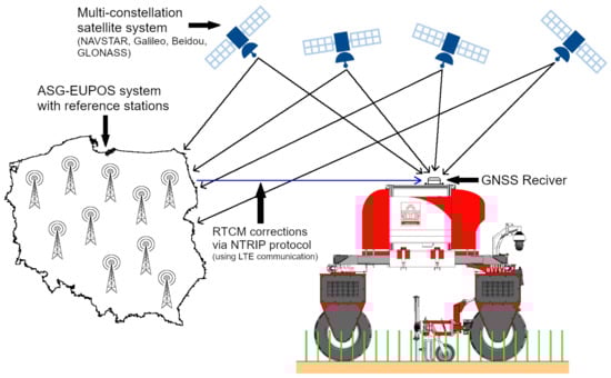
Figure 1.
General principle of RTK GNSS localisation with differential corrections using the ASG-Eupos infrastructure.
- Low accuracy (errors above one metre)—used for resource management, yield monitoring, and soil sampling;
- Medium accuracy (errors from twenty centimetres to one metre)—for tractor operator navigation with manual guidance;
- High accuracy (few centimetres of error)—for auto-guidance of tractors and machines performing precision operations.
The basic step for implementing a precision farming system is to purchase a GNSS receiver with the right localisation parameters. These parameters vary depending on the intended use case of the satellite receiver [19,20]. One of these use cases is the acquisition of data on agricultural area productivity. This involves collecting information on the amount of crops that are harvested at a particular location. Thanks to the known position and the measured amount of harvested material, it is possible to create a map showing the fertility of the area [21,22]. The use of satellite receivers in the measurement method not only improves the determination of the harvested area but also eliminates measurement errors [15].
GNSS-based localisation is used in precision agriculture for the application of crop protection products and fertilisers with variable application rates [23]. Fertilisation can be implemented based on pre-prepared application maps [24], which are developed based on satellite imagery analysis, multispectral imaging using drones, or agricultural area yield data [25]. GNSS-determined positioning allows for the creation of maps showing soil diversity and mineral abundance [24]. This information can be used to identify areas where intervention is necessary, e.g., due to disease outbreaks in the crop [19,25,26]. The use of satellite receivers enables the targeted application of plant protection products to areas where they are needed, reducing overlapping passes when spraying using an implement with a large working width [15].
In accordance with the European strategy to achieve climate neutrality, it is desirable to reduce plant protection products and other herbicides and replace them with mechanical treatments [27,28]. With the positioning accuracy of 2 cm that is provided by modern receivers, it is possible to reconstruct the map created while sowing, making it feasible to carry out mechanical weeding operations [23]. The main advantage of GNSS localisation over other systems used for precise positioning is its simple implementation and high accuracy [23,29]. Unlike vision systems, satellite positioning is insensitive to the visual appearance of the crop, shadows, weed density, and other factors closely related to crop expertise, such as disease incidence and changes in structure and colour at different stages of growth [29].
2.2. Guidance Systems for Agricultural Machinery
The introduction of precision farming techniques to a traditionally managed farm is, in most cases, gradual and economically justified. The leap from traditional to precision agriculture requires a large financial investment, which is not achievable for small- and medium-sized farms without appropriate investment plans [11,30]. Regardless of the level of implementation of precision agriculture tools, the implementation of assisted or automatic tractor guidance is a significant and inevitable step towards the complementarity of precision agriculture [11]. Guidance systems are crucial for achieving high levels of automation in agricultural machinery, where positioning accuracy plays a major role. Acquiring data on position, speed, direction of travel, and the current steering angle of the axle makes it possible to determine the movement of the vehicle, and this is the foundation for autonomous operation and precise control [11,17].
Guidance systems can be classified based on the level of automation in relieving the operator of driving the machine. These levels include manual, semi-automatic, and automatic systems [20,31]. Manual steering is based on visual indicators in the form of an LED bar or display indicating the deviation of the vehicle from its intended path [20]. The semi-automatic guidance system steers the vehicle autonomously during fieldwork, keeping the machine on a set path, which can be a straight line or a curve based on two points (start and end) [31]. The automatic guidance devices have the same functionality as semi-automatic ones, but they also have the ability to perform the turn itself; moreover, they can control the hydraulics of the implement’s suspension system and manage the attached implement [20,32]. The price of these devices depends on the quality and function of the equipment and the precision with which the positioning is performed. For example, the equipment can be supplied with an real-time kinematic (RTK) correction service enabling an accuracy of 2 cm. Alternatively, it can be supplied with another satellite-based augmentation system (SBAS) that achieves a lower accuracy of 20 to 50 cm [11,31,33]. Automatic guidance systems allow for accurate driving along a predetermined path and reduce the operator’s involvement in driving the vehicle, allowing them to focus on the operation being carried out [31,34].
Currently, there are several automatic guidance products available in the market with varying levels of sophistication. Budget solutions, such as FieldBee or Agribus-Navi [35,36], have fewer features and lower positioning accuracy than devices from leading manufacturers. Trimble is a major company that develops automatic guidance systems. Their NAV-900 series guidance controller, in the best configuration, can provide a positioning accuracy of 2.5 cm [33]. In combination with the GFX-750 display, the NAV-900 forms a complete system for precision farming. This system enables line guidance, turnarounds, control of implement sections, and input of variable rate application (VRA) maps [37,38]. The guidance system can control the steering in two ways: by fitting a dedicated steering wheel with an integrated servomotor or by connecting to the vehicle’s CAN network [33]. Topcon is another manufacturer of automatic guidance systems. Their AGS-2 controller, when used with an X-series console, offers features and functions similar to those of Trimble’s solution. One noticeable difference between these systems is the time it takes to determine an accurate position. Depending on the selected service providing RTK corrections, initialisation can take several seconds, and the resulting positioning precision is better than 2 cm [39]. The following example of commercial automatic guiding equipment is from John Deer, which offers the StarFire product series. Depending on the model and correction service selected, different localisation precisions of 15 to 2.5 cm can be achieved in times ranging from several minutes to a few seconds [40,41]. Also worth mentioning is a low-cost solution based on the open-source AgOpenGPS software. It allows for the construction of an automatic guidance system at home [20]. From this short overview, we can conclude that the commercial solutions offer high positioning precision and useful features for machine operators, but their disadvantage is the investment cost required to implement such a product. Additionally, these devices are closed systems that do not allow for expansion with devices from other manufacturers, and their adaptation to other types of machines, such as field robots, can be complicated or even impossible.
2.3. Advantages of GNSS Localisation Systems
The use of global navigation satellite system (GNSS)-based localisation in agriculture has many benefits, especially when work is carried out according to the concept of precision agriculture. Machine localisation makes it possible to use variable-rate application maps, which significantly reduce the use of plant protection products and fertilisers by applying them only where the crop requires them [34]. This has a positive effect on the environment by reducing its pollution and the poisoning of surface water. The reduced use of chemicals also brings economic benefits by reducing the cost of cultivation [34]. Another advantage of using positioning equipment with automatic control systems is the support of the machine operator. The technology not only improves the ergonomics of their work but also improves the efficiency of the operations performed by reducing the overlapping of two passes or leaving empty spaces between them. This translates into fuel costs, the amount of material used, the amount of crop harvested, and the effort put into the operation. For example, reducing the overlap of passes during herbicide application reduces herbicide use by up to 17% [34]. These problems are exacerbated in conditions of poor visibility or when working at night. The use of guidance systems reduces the impact of these factors, allows working hours to be extended during the day, speeds up work, and makes it easier to keep to the right time for carrying out agro-technical operations [34]. Studies carried out in Europe show that the use of precision positioning and navigation techniques allows one, when performing field work, depending on the type and size of the crop, to save between 6 and 8% of the costs incurred when performing agro-technical treatments in the traditional manner [20,34,42]. The result is an increase in crop profits of 23 to 30 EUR/ha [20,34].
2.4. Precision in the Execution of Agro-Technical Treatments
The improvement of sensing and localisation technology for agricultural applications has led to the use of robots partially replacing human sensory capabilities [2,43]. In the last decade, there has been a noticeable acceleration in the development of the field robots market. This, combined with other factors such as the difficulty in sourcing workers and the low efficiency of traditionally performed work, makes them an attractive alternative for farmers to increase the economic benefits of cultivation [14,44]. Mobile robots developed using state-of-the-art principles of probabilistic robotics [45] are likely to become indispensable in smart farms [44]. Field robots can be used for various agro-technical operations, including weeding, sowing, spraying, harvesting, disease detection, crop monitoring, and crop management [46].
The increasing popularity of field robots and precision farming is driving the demand for accurate agro-technical operations. The method of carrying out work is mainly based on satellite receiver positioning, which plays a significant role in performing treatments with high efficiency. It requires highly accurate receivers, but even then, the correct positioning of the implementing tools is not guaranteed [47]. Therefore, to achieve even greater efficiency and increase the precision of the work carried out, supporting systems based on various types of sensory systems such as vision systems, LiDARs, and colour sensors have been introduced into agricultural machinery [48,49]. An important advantage of these systems is that their operation is based only on local devices and is independent of the availability of satellite signals or mobile networks [47]. The work of these sensory systems consists of locally identifying the object and determining its position in order to precisely position the implement [48,49]. The precision of the agro-technical treatment carried out means the accuracy and care with which the tool performing the action is guided [46]. In the case of mechanical weeding in a plant row, the more precisely the tool is controlled, the closer to the plant it can work without risking damage to it. Recent research [46] has shown that, in practice, it is possible to achieve a tool positioning precision of around 1 cm depending on the support system used. The use of vision and LiDAR technology has limitations that are highly dependent on weather conditions. Variable lighting conditions, cloud cover, humidity, fog, or dust can significantly affect the quality of the sensory data, sometimes making it impossible to use these sensing modalities in the field operations [50].
Machine vision systems are most often based on standard RGB cameras, capturing images that are then analysed by advanced software [51]. The application of modern machine vision algorithms allows the desired effects to be obtained even with low-cost cameras, but this can be carried out by using different approaches [27,47,52]. One approach is to interpret the colour patterns acquired by the camera and then determine the objects of interest in the field of view [53]. For example, the use of adaptive RGB colour filtering makes it possible to identify pixels belonging to a plant in a wide area of lighting conditions and for a range of plant sizes [27,47,54]. This method of image analysis can be successfully used to guide a tool onto a row of plants (spraying) or between two adjacent rows (weeding) [27,53]. Another method of image interpretation can be based on the use of artificial intelligence algorithms and appropriately trained artificial neural networks [51,52,55]. This involves creating software capable of recognising objects based on specific criteria, such as the shape, colour, or external structure of the object. The advantage of this method is the ability to further retrain the network and improve its performance [51,52,55]. Software capable of recognising objects is the best way to position tools performing treatments directly within the plant [51]. Another support system responsible for the precise positioning of working tools is a system for analysing data recorded by a 3D space scanner—LiDAR [56,57,58]. The device enables objects to be accurately mapped in space in the form of a point cloud. The system can also make use of machine learning methods to distinguish between crops and weeds [57,58,59]. An unquestionable advantage of systems based on LiDAR-class sensors is their resistance to changing lighting conditions [57]. Plant detection could also be achieved using a true-colour sensor. This technology requires knowledge of the reflectance coefficients for different wavelengths [60]. With appropriate calibration, the system enables the recognition of plants from the early stages of growth. The advantage of this module is its low implementation cost, which creates an alternative to more expensive vision systems [60].
The aforementioned methods for the precise positioning of implements contribute to the quality of agro-technical operations and are an integral part of modern machinery adapted to precision farming [27,53]. For this reason, implements working with field robots are also equipped with them. Robots are technologically advanced machines with the ability to move along a predetermined path of travel with a high degree of accuracy [46], but it is the position of the tool and its individual control that most influence the quality of field operations [27,48].
2.5. Methods of Improving GNSS Positioning Accuracy
Determination of the position of self-propelled mobile platforms is mainly realised through the use of GNSS receivers. This results in the quality of the location being closely dependent on the number of visible satellites, atmospheric conditions, and signals providing differential corrections [47,61]. Although the GNSS allows for precise positioning at a level sufficient for the navigation of agricultural robotic applications, basing navigation only on the satellite system without adequate security or position filtering and algorithms to improve the reliability and stability of the position measurements obtained could cause errors. Therefore, various methods have been developed to additionally verify the satellite location through the use of filtering algorithms and other onboard devices that are the equipment of the machine [56,61,62].
GNSS-based navigation systems used during sensitive agro-technical operations must guarantee quality and safe operation. To ensure this, achieving the right level of integrity in the navigation system is a key factor. This integrity includes the ability of the system to provide timely warnings of malfunctioning hardware components, or a non-navigable position specified by the system. Therefore, integrity refers to the reliability of the information provided by the navigation system, especially when it is required to communicate to the user or the rest of the control system the occurrence of any failure at a specific time and with a probability of occurrence [63,64]. Receiver autonomous integrity monitoring (RAIM) was already invented in the early 1990s, long before satellite navigation was fully operational for civil use. Current RAIM techniques are based on various methods such as least-squares estimation and the use of classic and extended Kalman filters. The use of RAIM significantly increases the stability and confidence of positions determined by location-based devices [65,66].
Budget solutions to improve positioning accuracy presented in the literature typically involve the integration of inertial sensors. One such solution is to combine data from two low-cost GNSS receivers and an inertial measurement unit (IMU). In this case, the used receivers take into account the RTK correction provided by a free-of-charge open service. With the appropriate software and the use of the extended Kalman filter (EKF) method of filtering the data in the example described, the researchers in the field obtained higher accuracy in the time base even when one of the receivers did not receive the RTK correction [67]. However, many GNSS receivers do not have an integrated IMU, while the integration of an external one can be problematic, e.g., because of the required isolation from the mechanical vibrations of the agricultural robot.
Another method of supporting position determination can be the use of a simultaneous localisation and mapping (SLAM) algorithm with passive cameras or laser scanners (often referred to as LiDARs). Depending on the main sensing modality being used, SLAM can be divided into LiDAR SLAM or visual SLAM [59,68,69]. GNSS support by LiDAR SLAM enables a more accurate estimation of the machine’s position by tracking the machine’s trajectory (LiDAR odometry), using static elements of the environment as a reference to determine the machine’s pose [59,70]. Through the use of data fusion and filtering or optimisation algorithms, it is possible to achieve high positioning precision even when satellite signals are difficult to access [62,69]. Visual SLAM has a similar operating principle but requires the implementation of image analysis procedures that track stationary, salient objects in the environment and make it possible to estimate the camera’s pose [71]. Its advantage over LiDAR SLAM is a much lower cost resulting from the replacement of an expensive laser scanner with a standard RGB camera [72].
However, visual SLAM, or its simplified version, called visual odometry [68], requires identifiable objects within the field of view of the camera for effective pose tracking [59]. Hence, this approach is successfully used in agriculture when working in man-made environments (e.g., greenhouses) or near buildings, which often interfere with the correct operation of GNSS receivers by their presence [73]. The operation of such a system appears to be difficult in large-area fields where there are difficulties in identifying stationary objects, but these solutions continue to be of interest to researchers who are looking for hardware and software improvements to adapt SLAM to work properly in open spaces [56,74].
3. Experimental Evaluation of GNSS Localisation under Field Conditions
3.1. Motivation for the Experiment
The significant increase in the benefits of using GNSS receivers for crop management is causing the search for different hardware and software solutions to achieve high-precision positioning. Many of the positioning devices available on the market perform well in field conditions, but these are mainly equipment designed for agricultural use and are highly priced. To increase the availability of precision farming solutions for smaller farms, it is necessary to consider the trade-off between sufficient accuracy and the price of the components used [61]. In addition, due to environmental regulations imposed by the European Union [28], more and more farms are forced to introduce costly solutions to reduce the use of chemicals, increasing the use of ecological farming methods. Taking the above factors into account, machine positioning measurements have been carried out using GNSS receivers in various configurations and compared with measurements taken with a commercial high-precision device as a reference signal source.
3.2. Experimental Setup and Environment
The experiment was carried out using a field robot, which is an electric development unit used to carry out the research and functional testing of systems designed for precision agriculture (Figure 2).
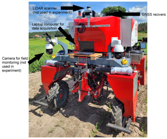
Figure 2.
Electric field robot for seeding and weeding used in the experiment with additional sensors.
The machine was designed in line with current trends among robots performing agro-technical operations in the field. It is a device that uses a commercial satellite receiver, developed for tractor guidance, to move independently along the technological path, but any system with the appropriate communication protocol can be connected for this purpose. However, for the purpose of the experiments, the vehicle was driven manually from a remote control operated by an operator. The experiment was carried out in July under field conditions on an agricultural field of approximately 0.6 hectares (Figure 3A) with a maize plantation in the early stages of growth at the 3–4-leaf level. The experiment was conducted on flat terrain that had small local depressions and was moderately wet, without causing excessive machine perching or pollination. The experiment was implemented in a location close to the Poznań metropolitan area (Figure 3B), which benefits from good coverage and quality of the ASG-Eupos and GSM networks signal.
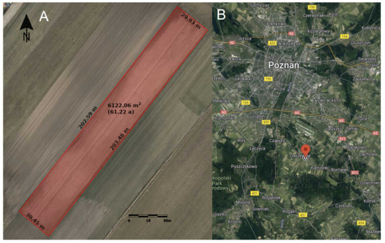
Figure 3.
Dimensions of the field in which the experiment was carried out (A) (measured with online application [75]) as well as the exact location of the field on a larger-scale map (B) [76].
The research was carried out using three GNSS receivers in different configurations. Each of these devices used signals from multiple satellite constellations such as GPS-NAVSTAR, Galileo, Beidou, and GLONASS during positioning. This results in improved accuracy as the GNSS receivers operating in the differential mode are able to rely on more satellites to determine their location. Furthermore, RTCM corrections provided by the ASG-Eupos system, which consists of a network of reference stations located throughout Poland at regular distances, were passed to receivers. The corrections were transmitted using the Networked Transport of RTCM via Internet Protocol (NTRIP). The Internet network was accessed using LTE communication (c.f. Figure 1).
The first receiver is the AGS-2 manufactured by Topcon. This is a device designed for the precise positioning and guidance of agricultural tractors on arable fields. It has an integrated inertial module with a three-axis accelerometer, gyroscope, and magnetometer. It features high performance and allows for positioning with an accuracy of 1 cm in RTK-Fix mode. NTRIP correction data from the ASG-Eupos service were supplied to the receiver. Position data from the AGS-2 were transmitted via the serial bus at 10 Hz in the form of NMEA protocol GGA messages and stored on the measurement computer. During the experiment, the readings of this receiver were used as a reference.
The second receiver used in the experiment was assembled from two u-blox ZED-F9P modules, one of which operates as a moving base (MB) and the other as a rover. The moving base, via a serial bus, transmits RTCM correction data to the rover receiver, so it is possible to obtain the precise relative distance between the two receivers, as well as data of the direction in which the machine is facing (heading). NTRIP corrections from the reference station provided by the ASG-Eupos system [77] are transmitted as input to the moving base receiver. This makes it possible to obtain the receiver’s absolute position with RTK-fix-level accuracy. According to the manufacturer of this receiver, a positioning precision of 0.01 m + 1 ppm is possible. Position data were transmitted from the receiver at a frequency of 10 Hz.
The third receiver that was used during the experiment was a single u-blox ZED-F9R module, which is similar to the ZED-F9P module but not adapted for moving base operation. Its firmware allows for sensor data fusion using a 3D inertial measurement unit (IMU) from ST Microelectronics—the LIS2DH12 model. This IMU is, by default, built into the PCB that operates the GNSS receiver, making ZED-F9R the easiest to use and most cost-effective GNSS receiver from the u-blox range available at the moment of conducting our experiments. As in previous cases, NTRIP corrections provided by the ASG-Eupos service were transmitted to the receiver. The positioning accuracy of this device as declared by the manufacturer is 0.01 m + 1 ppm. Measurements were taken and recorded at 5 Hz.
The experiment was carried out by making two passes. The first one was a short one with one turn without crossing trajectories, and the second one was a longer run representing a typical trajectory of an agricultural machine during an agro-technical treatment. The receivers were mounted on top of the machine, not obscured by other machine components. All receivers were mounted in the line of symmetry of the vehicle offset from each other along one axis (Figure 4). The sky during the experiment was briefly cloudy.
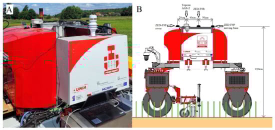
Figure 4.
Position of the antennas of the three GNSS receivers used in the experiment, a photo showing the actual placement (A), and a schematic arrangement with the exact dimensions between the receivers (B).
4. Results of GNSS-Based Localisation
The data measured during the field tests for each of the receivers were stored on the measuring computer in separate files and contained information about the time of the measurement taken, the geographical coordinates in the WGS-84 system (World Geodetic System ’84), and the direction of movement of the vehicle. These data were then converted to a common reference system, which was the Topcon AGS-2 reference receiver. The next step was to convert the measured values from the WGS-84 geographic coordinate system to the Universal Transverse Mercator (UTM) standard, performed to better reproduce and present the measurements taken. Two toolkits for processing the datasets and their evaluation were used to analyse the results.
One of these toolkits is evo [78], a Python package for the evaluation of odometry and SLAM results, which provides procedures for handling, evaluating, and comparing trajectories estimated by odometry or SLAM algorithms. The evo toolkit supports several trajectory formats, including the ROS bagfiles used in our experiments, and offers configurable algorithmic options for association, alignment, and scale adjustment of the compared trajectories. The second set of tools are the scripts included in the TUM RGBD Benchmark dataset [79], which, although older and less automatised than evo, offer a detailed visualisation of the errors between the ground truth and the estimated trajectory.
To assess the precision of the reconstructed trajectories, the absolute trajectory error (ATE) method is employed. This technique, along with its associated error metric, was originally presented in [79] and has since become widely adopted in robotics research. The ATE value is determined as the Euclidean distance between the corresponding points of the estimated trajectory and the ground truth trajectory. Consequently, the ATE metrics provide insights into the deviation of the estimated pose along the trajectory from the reference pose. For the entire trajectory, the root mean squared error (RMSE) of the ATE metrics is computed. Assuming that two trajectories are given—the ground truth one , and the estimated one , with the same number of n GNSS receiver poses—and that and are given as 4×4 homogeneous matrices, we can compute the ATE metrics for the i-th frame:
and then obtain the ATE value for the whole trajectory from the RMSE of (1) for all GNSS poses. It is important to note that, to ensure accurate ATE calculations, the trajectories must be aligned beforehand by identifying a transformation that minimises the distance between the two rigid sets of points representing these trajectories (1). In the first step of processing the input trajectories, pairs are created between the compared GNSS poses based on their time stamps. Then, based on the related points, the considered trajectories are aligned using the Umeyama algorithm [80]. The next step is to calculate the differences between each pair of points, and the results of the position errors are presented as mean, median, and standard deviation. Finally, graphs are generated showing the trajectories under consideration, together with a display of the position errors at each section of the route. Both toolkits used in the presented experiments are equipped with procedures for calculating the absolute trajectory error according to the definition given by (1); however, in evo, this metric is called absolute pose error (APE). To remain consistent with the plots generated by evo, we will use the APE acronym throughout this paper.
As mentioned above, two measurements were carried out and analysed separately. The first measurement consisted of a shorter pass with one turn (Figure 5). The figure shows the overall trajectory of the first pass superimposed on the field map from the three GNSS receivers. The resulting trajectories were compared with the reference trajectory using the evo tool, and the measurement deviation results for the individual receivers are summarised in Table 1.
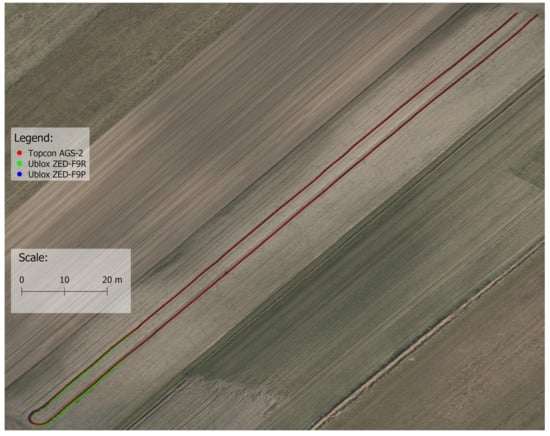
Figure 5.
Representation of measured trajectories on a field map.

Table 1.
APE of trajectories measured during the first run by individual receivers compared with the measurement from the AGS-2 receiver, where RMSE—root mean square error, mean—arithmetic average, median—middle value, std—standard deviation, min—minimum value, max—maximum value, SSE—sum of squared errors.
Based on the data presented, it can be seen that the configuration of the localisation system using the ZED-F9P receiver resulted in notably higher accuracy. The smallest measurement error obtained was less than 1 cm, and the average error from the entire run did not exceed 5 cm. Figure 6A shows a comparison of the measurement from the first run made with the ZED-F9P receiver with the reference trajectory. The presented pass trajectory illustrates the occurrence of the largest deviation when passing the headland at the end of the field. On the other hand, Figure 6B shows the error of the measurement made during the first pass with the ZED-F9R receiver. The position error of the trajectory under consideration has been marked using a colour scale. It can be seen from the figure that the largest error of this receiver was registered in the area before the turnaround. However, deviations exceeding the determined average are also noticeable in other parts of the trajectory.
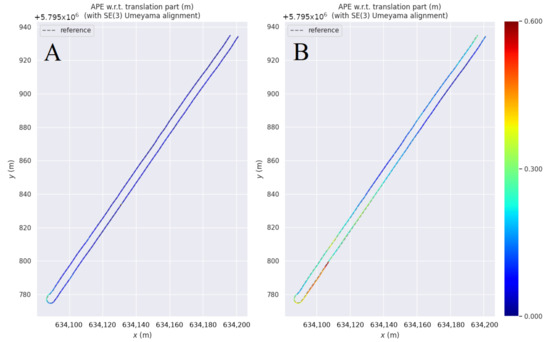
Figure 6.
Absolute pose error along the entire length of the trajectory estimated from the ZED-F9P receiver (A) and the ZED-F9R receiver (B).
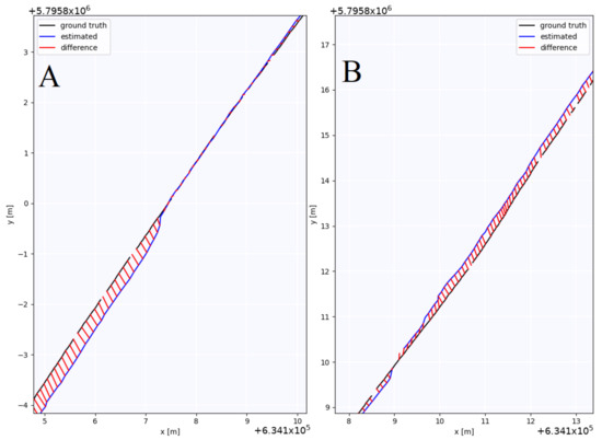
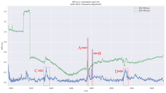
For the trajectories presented above, graphs have been generated to show the evolution of the absolute position error as a function of time. Figure 7 depicts this visualisation for the ZED-F9P receiver. From analysing the characteristics in Figure 7, it is evident that the ZED-F9P receiver’s measurement displays a momentary and significant inaccuracy of approximately 60 cm at the 220th second of the measurement, which is marked in the figure with the letter A. The section marked A in Figure 7 is illustrated in detail in Figure 8. Based on the detailed plot shown in Figure 8, with precise labelling of measurement points, it can be inferred that the error resulted from a momentary loss of data in the receiver operating in moving base mode, causing a temporary drop in the heading to zero.
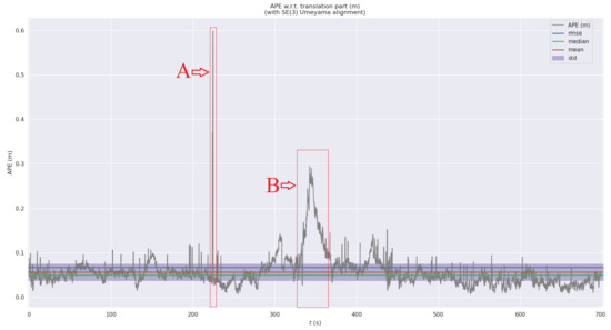
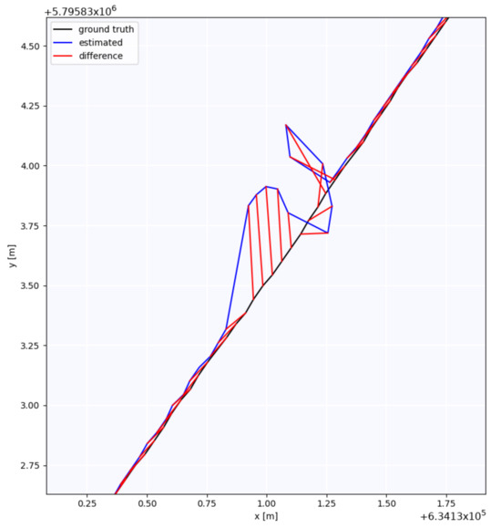
Figure 8.
Detailed illustration of a section of the trajectory determined by the ZED-F9P receiver during the first run, with the exact marking of the associated measurement points.
Figure 9 presents a detailed view of the analysed trajectory during the turning procedure. This segment was captured between 320 and 360 s of measurement, which is marked by the letter B in Figure 7. In the previously presented characteristic in Figure 7, there is a noticeable increase in the position error, which reached a maximum of 0.3 m and then started to return to values similar to the estimated position’s standard deviation. By referring to Figure 9, it becomes apparent that the error of the measured trajectory intensified as the machine initiated the turning stage. As the machine passed through the curve, the error gradually increased. Only at the end of the turnaround, when the machine began to drive on a relatively straight line again, did the position error slowly decrease. This effect observed in this measurement setup may be due to the fact that the data are only acquired from the GNSS receiver, without being combined with data from the machine’s steering system or inertial unit. Maintaining the consistency of measurement between consecutive points along the designated course results in an insufficiently dynamic response of the measurement set.
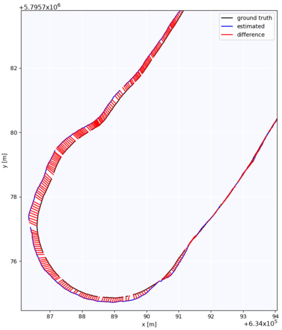
Figure 9.
Detailed illustration of a section of the trajectory at the turning area determined by the ZED-F9P receiver during the first run.
The characteristics of the trajectory measurement conducted using the ZED-F9R receiver vary over time, as presented in Figure 10. The measurement performed is characterised by a large variation in the absolute position error over the course of the run. Furthermore, noteworthy spikes are visible, which may significantly disrupt the accurate control of a machine that is positioned based on the analysed measurement set.
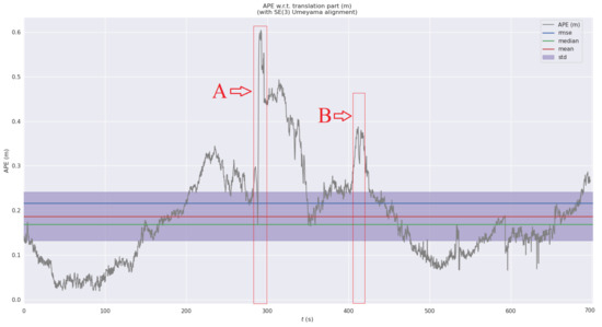
Figure 10.
Absolute position error estimated from the ZED-F9R receiver for the first pass in the time domain.
Temporary terrain unevenness causes machine tilting, resulting in fluctuations that directly impact the position of the GNSS receiver mounted on top of the machine. The 230 cm height at which the receiver is mounted further exacerbates this negative effect. Examples of these effects are shown in Figure 11. Diagram A corresponds to the section marked A in Figure 10, while diagram B presents in detail section B from Figure 10.
The second measurement taken during the field tests reflected the typical agro-technical activities carried out in the field. Figure 12 shows the complete route of the second passage overlaid onto the map of the field using data from the three GNSS receivers. Following the same procedure as in the first measurement, Table 2 presents the outcomes of analysing the absolute position error for both receivers in relation to the reference receiver.
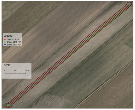
Figure 12.
Representation of measured trajectories during the second run on a field map.
Table 2.
APE of trajectories measured during the second run by individual receivers compared with the measurement from the AGS-2 receiver, where RMSE—root mean square error, mean—arithmetic average, median—middle value, std—standard deviation, min—minimum value, max—maximum value, SSE—sum of squared errors.
The results of the absolute position error calculations presented in Table 2 indicate that, similarly to the first case, the system with the ZED-F9P receiver demonstrated superior accuracy compared to the reference receiver. The smallest measurement error obtained was only at the level of a few millimetres, whilst the average error across the entire run was approximately 6 cm. Conversely, results obtained from the ZED-F9R receiver significantly deviated from the expected outcomes. The minimum error achieved during testing clearly exceeded 10 cm, and, in extreme cases, was almost 1.5 m. The average value of the absolute position error exceeded 40 cm, which was higher than anticipated.
Figure 13A illustrates a comparison of the overall trajectory recorded with the ZED-F9P receiver and the reference trajectory. A corresponding comparison was generated for the ZED-F9R receiver (Figure 13B). Both Figure 13A,B were produced with the evo tool. Figure 13A,B visualise the absolute position error at each point during the passage on a colour scale. The error varied over time in both cases, as evidenced by the graph in Figure 14. To facilitate a comparison of the error progression for the two receivers utilised, the data are presented in a unified graph. The X-axis denotes the timestamp at which each measurement point was captured in UNIX time format.
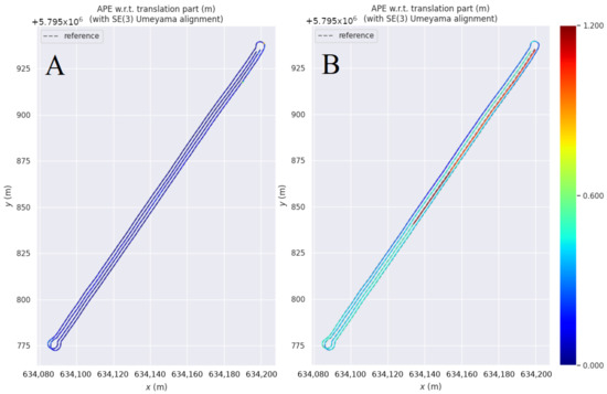
Figure 13.
Absolute position error over the entire length of the second experiment trajectory estimated by the ZED-F9P receiver (A) and ZED-F9R receiver (B).
According to Figure 14, the ZED-F9R receiver shows a significant absolute position error when starting to acquire positioning. Multiple factors can influence measurement precision in this case, such as incorrect receiver configuration, temporary loss of correction data, a low-quality inertial unit and its inaccurate positioning, or challenging terrain. The imprecision resulting from the initial measurement error led to inaccurate localisation data collected by the receiver for almost 200 s. As the experiment progressed, the system gradually improved its positioning accuracy. Nevertheless, the receiver displayed significant instability, resulting in notably poorer positioning quality when compared to the ZED-F9P receiver. The receiver, comprising two modules—moving base and rover—demonstrated better performance while conducting the experiment. The recorded measurement disturbances were insignificant in magnitude and brief in duration. However, from the overall characteristics, it is possible to determine the sections where the error of the estimated position was larger. These fragments are marked in Figure 14 with rectangles labelled A to D. An extensive illustration of the two most significant immediate position errors can be found in Figure 15A,B—these correspond to the fragments of absolute estimated position error shown in Figure 14 and are labelled as A and B. Furthermore, the rectangles labelled C and D in Figure 14 represent the error of the measured trajectory in the area of the turnaround detailed in Figure 16.
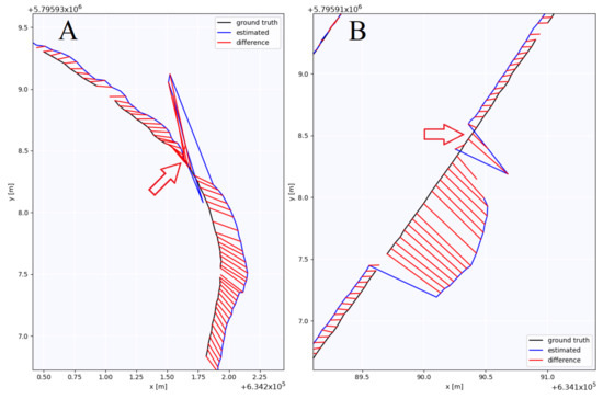
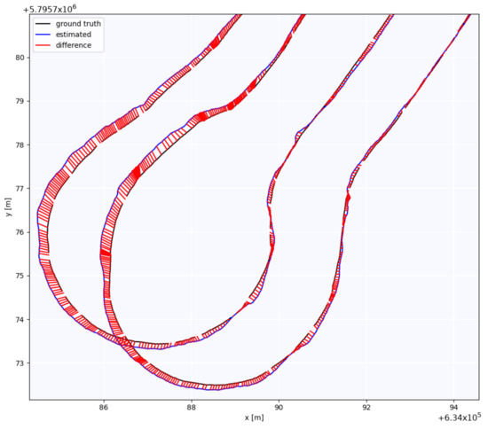
Figure 16.
The absolute position error of the estimated trajectory near the turnaround, measured by the ZED-F9P receiver during the second run.
Figure 15 shows segments of the estimated trajectories with an instantaneous significant measurement disturbance. In the figures, corresponding measurement points of the anticipated trajectory and ground truth are indicated. A marked, sudden rise in absolute position error can be observed in Figure 15A,B at the points marked with arrows. This was caused by a brief data loss from the moving base module, leading to a drop in the estimated heading to 0.
Furthermore, examining the measurements collected using the ZED-F9P receiver, it can be noted that, in several places, the estimated position error surpasses the mean values. These are fragments of the trajectory depicting the turning performed by the machine. The increase in measurement error commences as the machine turns, persisting until it returns to a straight line. A visual demonstration of this case within one of the headland areas is shown in Figure 16.
5. Correcting GNSS Trajectories with Visual Odometry
The literature survey and the results of our experiments suggest that the GNSS-based localisation of an agricultural robot raises several issues related to the characteristics of the environment and the used GNSS equipment. Some of the problems that we have observed in the experiments, such as outlier robot poses generated when RTCM corrections are temporarily unavailable, can be rectified using an auxiliary localisation system based on external measurements. The integration of visual [81] or light detection and ranging (LiDAR) odometry [72,82] with GNSS localisation stands out as a notable strategy within this domain [69]. LiDAR-based systems offer high precision and robustness [70], but high costs and maintenance expenses dissuade the adoption of sensors like 3D LiDAR. Moreover, the absence of readily discernible prominent features and the dynamic characteristics of vegetation-covered regions, with low repeatability in feature detection, diminish the efficacy of LiDAR-based localisation methods in field applications [68].
Visual solutions, relying on passive cameras, are generally more cost-effective, and rely on photometric features, which are present in most of the environments [83]. In particular, the integration of monocular visual odometry, leveraging a single camera to infer the robot’s movement by tracking visual features in the surroundings [84], emerges as a cost-effective complement to GNSS. Direct visual odometry, a technique that directly estimates motion by minimising pixel-wise intensity differences between consecutive frames [85], provides dense and continuous motion estimates. However, direct methods can be sensitive to changes in lighting conditions and may struggle in scenes with low texture or repetitive patterns. On the other hand, feature-based visual odometry [86], offers a more sparse but potentially robust solution, proving advantageous in challenging scenarios where direct methods may falter. Feature-based approaches are often more resilient to variations in lighting and can handle environments with limited texture, making them suitable for a broad range of real-world applications.
5.1. Low-Cost Visual Odometry as External Localisation Method
Monocular visual odometry relies on visual information obtained from a single camera to track the robot’s movement over time. Despite its utility, monocular visual odometry faces limitations such as scale ambiguity, sensitivity to lighting conditions, and challenges in handling dynamic scenes [84]. Therefore, our solution for the integration of GNSS localisation and visual odometry relies on the open-source ORB-SLAM3 library [71,87], which addresses these challenges by using ORB (Oriented FAST and Rotated BRIEF) features that excel in real-time applications, providing reliable and accurate tracking even in environments with varying illumination. Its ability to build and optimise a map of the surroundings, coupled with the integration of keyframe-based optimisations, makes ORB-SLAM3 a widely adopted solution for monocular visual odometry applications [69,71].
The ORB-SLAM3 software was adopted for localisation in large-area fields by setting its parameters according to the results of preliminary experiments and by reducing the size of the input camera image in such a way that the sky is no longer visible and the point features are detected only below the horizon line (Figure 17A). This simple modification prevents the tracking thread of ORB-SLAM3 from focusing too much on features located far away (e.g., on some trees just above the horizon line), which tend to be weak in terms of saliency and detection repeatability, and increases tracking robustness in our scenario (Figure 17B).
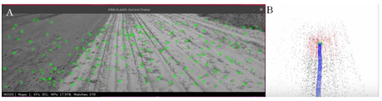
Figure 17.
Visualisation of the ORB point features (green) detected by ORB-SLAM3 in the reduced image (A) and the point features tracked in the map (red/black) with the camera trajectory (blue) (B).
Whereas for full simultaneous localisation and mapping (SLAM) operation, ORB-SLAM3 detects and closes loops in revisited places, we do not apply loop closing in our system. The reasons are twofold: firstly, sparse and unevenly distributed point features in the vegetation-covered surroundings, with few salient objects in the camera’s field of view, make the loop detection mechanism unreliable; secondly, we apply the localisation constraints from ORB-SLAM3 only locally, exploiting the robust visual tracking abilities of ORB-SLAM3 while avoiding problems with the drift and scale changes that might appear prominently with unreliable loop closing and re-localisation.
The presented solution directly draws from our previous work on LiDAR-SLAM and GNSS integration [88], using the factor graph formulation of the robot trajectory estimation problem with pose constraints from two different sources. In this solution, the 6-DOF transformations produced by ORB-SLAM3’s visual odometry contribute to the construction of constraints. Notice that we have directly used the built-in camera of the laptop attached to the agricultural robot for the presented experiment as the sensor yielding the images to feed the visual odometry pipeline. Hence, our solution is extremely low-cost, as it needs no additional equipment to be deployed on the robot.
5.2. Integration Applying Factor Graph
The trajectories obtained from visual odometry and GNSS data were integrated using a factor graph representation, which provides a convenient way of estimating the robot pose using more than one data source. The mentioned graph consists of multiple nodes and edges [89]. Each node represents the pose of the robot at a given time, while edges provide constraints that connect subsequent poses and define the transformation between them. The overall structure of the constructed factor graph is presented in Figure 18.
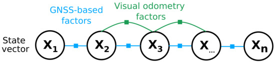
Figure 18.
The overall structure of the factor graph. It consists of nodes that represent state vectors of a robot and edges that constitute constraints coming from GNSS and visual odometry system.
The estimated state vector for the i-th pose is denoted as and contains a 6-DOF pose of a robot that consists of a rotation matrix and translation vector :
The factor graph is created primarily based on GNSS data, as new nodes and edges are added every time the new GNSS positioning message is received. The initial values for each vector state, which are used in the process of factor graph optimisation, also originate from GNSS measurements. This is because the information from visual odometry is only added in the case of the degraded accuracy of GNSS positioning. Thanks to this approach, the estimated trajectory is coming from the satellite navigation system for the vast majority of the time, and thus it is not susceptible to such problems as the pose and scale drift.
However, there are multiple situations when the GNSS accuracy can be degraded and become temporarily insufficient for precision farming applications. For that reason, our approach is to detect these moments and to appropriately integrate the information from the visual odometry system. The decision on whether to integrate the odometry measurements in the factor graph is taken based on the variance of GNSS data. The variance of the GNSS receiver pose (i.e., the robot pose) can be either calculated based on past measurements or read directly from the u-blox GNSS receiver. In our case, we use the second method, as it is more accurate and does not require any additional computations to create the covariance matrix related to the GNSS position. In the RTK mode, the value of variance for axes, which was reported by u-blox receivers during the conducted experiment, was very similar in all axes, and at the level of [m2]. Any significant deviation in these values is an indication of degraded accuracy and thus results in adding the visual odometry measurements to the factor graph. This allows us to optimise the trajectory only when necessary in order to improve the overall localisation accuracy. The measurements from both the GNSS and odometry are included in the factor graph in a similar way. The poses, obtained from these systems, are used to calculate the increments between subsequent graph nodes and are then added to the graph as edges. In the case of GNSS data, the error function used during the optimisation has the following form:
where , are 6-DOF poses of a robot coming from the GNSS trajectory. The data from the ORB-SLAM3 system are integrated analogously; however, this requires some additional steps. The first of them is to synchronise the measurements with GNSS data. To achieve that, the correspondences between poses from both systems are found based on their timestamps. The second step is to find the scale of the visual odometry trajectory, as the monocular SLAM system used in our experiments does not provide such information. This step is performed using the Umeyama algorithm [80], similar to ATE metrics computation (see Section 4), as it minimises the error between the past GNSS and ORB-SLAM3 trajectories to calculate the scale value. It also aligns the two trajectories together, which makes it possible to estimate the transformation between both system coordinate frames. What is more, it also provides information about the standard deviation of visual odometry poses (relative to the RTK GNSS data), which is further used to compute the covariance matrix () required in factor graph optimisation. After these steps are completed, the selected parts of the ORB-SLAM3 trajectory can be integrated into the factor graph when necessary. An error function in this case is defined as follows:
where , are 6-DOF poses of the robot coming from the visual odometry system. The result of optimisation of the described factor graph is the estimated value of the state vector corresponding to each node. As mentioned before, in our case, it is the pose and orientation of a robot. The optimisation itself is performed using the g2o [90] library, which, using the graph structure, minimises the sum of squared errors of all edges in the graph:
where is an error function corresponding to each edge type and , are sets of the factor graph nodes with GNSS-based and visual odometry constraints, respectively.
5.3. Correction Results
In order to verify the effectiveness of the proposed approach to GNSS trajectory correction, the trajectories recorded using the ZED-F9P receiver were integrated with the visual odometry measurements. As already described in the previous sections, the GNSS data are affected by some random disturbances of the provided position that can be potentially improved using the optimisation technique. An exemplary part of the trajectory, where GNSS accuracy was reduced but ORB-SLAM3 provides reliable pose tracking, is presented in Figure 19A. At the same time, Figure 19B shows the value of the variance of individual coordinates yielded by the GNSS receiver. Based on these plots, it can be seen that disturbances in satellite system positioning can be detected by monitoring their variance. For that reason, every such situation triggers the integration of visual odometry measurements, which means that, after transforming and synchronising the ORB-SLAM3 trajectory to the GNSS data, it is added to the factor graph.
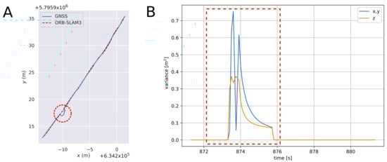
Figure 19.
(A) Comparison of a fragment of the GNSS and ORB-SLAM3 trajectories. The red circle marks the spot where the GNSS positioning accuracy was degraded but the ORB-SLAM3 system provides accurate pose estimation. (B) The variance in coordinates is provided directly by the receiver. The part of the plot contained in the red rectangle in Figure (B) corresponds to the part of the trajectory marked in the red circle in Figure (A).
An effect of such trajectory correction is presented in Figure 20. It shows an exemplary part of the robot’s path before and after the optimisation, and the disturbance marked in the red circle corresponds to the disturbance presented in Figure 19.
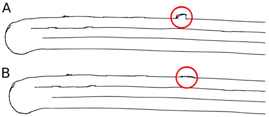
Figure 20.
(A) Estimated trajectory before adding constraints coming from the visual odometry to the graph. (B) Trajectory after the optimisation, which improved the fragment with visible positioning disturbances marked in the red circle.
The numerical values of ATE, calculated after applying the trajectory corrections using the factor graph approach, are presented in Table 3 and Table 4. They correspond to the trajectories recorded during the first and second runs performed during the experiment, respectively.
Table 3.
APE of trajectory measured during the first run by ZED-F9P receiver. The trajectory was improved by integrating the visual odometry measurements using the factor graph approach.
Table 4.
APE of trajectory measured during the second run by ZED-F9P receiver. The trajectory was improved by integrating the visual odometry measurements using the factor graph approach.
When compared to Table 1 and Table 2, which contain the analogous results but before optimisation, it can be seen that the biggest improvement is visible in the case of the max value of the error. The improvement in the remaining columns is rather marginal. The reason for such results is the fact that a relatively short part of both trajectories was affected by the disturbances and thus the overall accuracy did not change significantly. However, there are precision farming applications where even a few incorrect robot positions can have a noticeable effect on the results. In such cases, the presented approach allows us to detect and reduce the GNSS disturbances as it significantly decreases the maximal value of an error of the estimated trajectory.
6. Conclusions
Precision positioning systems are increasingly prevalent in modern agriculture, with smaller farms showing growing interest despite their primary concern being the cost of hardware components. Consequently, there is a persistent need for positioning solutions that offer satisfactory accuracy at a reasonable price. The intensification of ecological farming methods and restrictions on chemical usage prompt farmers to adopt precise positioning devices. The rapid development of field robots for agro-technical operations further drives the demand for affordable precision positioning equipment. As agriculture’s future demands more from positioning systems, they become indispensable for farm management, necessitating further advancements to enhance their effectiveness.
In the context of these requirements, the practical value of the experiments showcased in this paper lies in their ability to validate and optimise precision positioning systems for real-world agricultural applications. By conducting empirical studies under field conditions, the experiments provide insights into the effectiveness and reliability of GNSS-based localisation technologies, such as the ZED-F9R receiver system and visual odometry integration. Our experimental data show that, when contrasted with the reference trajectory, the employment of a ZED-F9P receiver system featuring two modules—one functioning in moving base mode and the other in rover mode—resulted in an acceptable positioning accuracy. However, this solution is more expensive than the ZED-F9R system, as two receivers must be purchased. Nevertheless, the cost of the ZED-F9R system is dependent on the inertial module, whose price ranges from a few to several thousand euros. The IMU used in our experiments was a low-cost, low-quality device, which undoubtedly affected the accuracy of the measurements taken with the ZED-F9R receiver module. Replacing the default inertial unit with a higher-performance one would enhance the quality of the data obtained. The indications of absolute position would be improved, alongside more precise orientation. However, it should be noted that this orientation will not be as accurate as determined by the ZED-F9P modules. The positional accuracy of the data obtained from the ZED-F9P receiver measurement system was satisfactory for most agricultural treatments despite temporary and minor positional errors.
An important lesson learned from our experiments is the commendable performance of visual odometry over short distances, despite utilising extremely low-cost hardware (a laptop with its built-in camera). This allowed the integration of visual odometry pose estimates to effectively counteract observed short-time periods of degraded GNSS accuracy. Additionally, we have demonstrated the feasibility of factor-graph-based integration between the GNSS and visual odometry in a real-time localisation system. The showcased results suggest that visual odometry holds significant potential for a wide range of applications in agriculture. Specifically, it can be particularly useful for field robot navigation along pre-planned paths and for self-propelled machines, such as TMR mixers. These systems can be even more effective when operating in close proximity to buildings. In instances of GNSS signal or correction data loss, integrated visual odometry seamlessly provides accurate enough pose estimates, ensuring the safe continuation of planned agricultural operations.
Further development of visual or LiDAR odometry-based localisation in agriculture faces several challenges. These include identifying specific features in fields, such as localised clusters of vegetation, and extending the measurement range by utilising ambient feature points around agricultural fields. Currently, the lack of clear, characteristic, stationary reference points for distance measurements presents a significant challenge. An intriguing solution could involve implementing this method in intercropping, where various plant types are grown in close proximity, serving as reference points for field robots equipped with visual odometry systems. Additionally, future research could involve conducting experiments using visual odometry in varying lighting and environmental conditions, including different weather conditions such as cloud cover, rain, and wind. Clear recommendations regarding the applicability of vision or LiDAR-based odometry as a means of complementing GNSS-based guidance for specific types of agricultural treatments (e.g., tillage, seeding and planting, fertilisation, pest and weed control) may offer practical value. However, reaching such conclusions will require further intensive field experiments.
Author Contributions
Conceptualisation, M.N. and P.S.; methodology, M.N. and P.S.; software, M.N. and K.Ć.; validation, P.S., M.Z. and S.S.; formal analysis, P.S. and M.Z.; investigation, M.N.; resources, M.N., P.S., K.Ć. and S.S.; data curation, M.N. and K.Ć.; writing—original draft preparation, M.N. and K.Ć.; writing—review and editing, P.S., M.Z., M.N. and S.S.; visualisation, M.N. and K.Ć.; supervision, P.S. and J.W.; project administration, P.S. and J.W.; funding acquisition, J.W. All authors have read and agreed to the published version of the manuscript.
Funding
The research was conducted by Ph.D. students under the Applied Doctorate Programme of the Polish Ministry of Science and Higher Education, realised in the years 2022–2026 (Agreement No. DWD/6/0046/2022), 2020–2024 (Agreement No. DWD/4/22/2020) and 2021–2025 (Agreement No. DWD/5/0016/2021). P.S. and K.Ć. were supported by Poznań University of Technology internal grant 0214/SBAD/0242.
Institutional Review Board Statement
Not applicable.
Informed Consent Statement
Not applicable.
Data Availability Statement
The experimental data used in this paper and the corresponding source code are publicly available at GitHub: https://github.com/MatNij/AgroLoc2024 (accessed on 4 March 2024).
Conflicts of Interest
The authors declare no conflicts of interest.
References
- Kulkarni, A.A.; Dhanush, P.; Chetan, B.S.; Gowda, T.; Shrivastava, P.K. Applications of Automation and Robotics in Agriculture Industries; A Review. In Proceedings of the International Conference on Mechanical and Energy Technologies (ICMET), Nanjing, China, 28–30 June 2019. [Google Scholar]
- Marinoudi, V.; Lampridi, M.; Kateris, D.; Pearson, S.; Sorensen, C.G.; Bochtis, D. The Future of Agricultural Jobs in View of Robotization. Sustainability 2021, 13, 12109. [Google Scholar] [CrossRef]
- Jurišić, M.; Plaščak, I.; Barač, Ž.; Radočaj, D.; Zimmer, D. Sensors and Their Application in Precision Agriculture. TehniČKI Glasnik 2021, 15, 529–533. [Google Scholar] [CrossRef]
- Paul, K.; Chatterjee, S.S.; Pai, P.; Varshney, A.; Juikar, S.; Prasad, V.; Bhadra, B.; Dasgupta, S. Viable smart sensors and their application in data driven agriculture. Comput. Electron. Agric. 2022, 198, 107096. [Google Scholar] [CrossRef]
- Vera, J.; Conejero, W.; Mira-García, A.B.; Conesa, M.R.; Ruiz-Sánchez, M.C. Towards irrigation automation based on dielectric soil sensors. J. Hortic. Sci. Biotechnol. 2021, 96, 696–707. [Google Scholar] [CrossRef]
- Guo, J.; Li, X.; Li, Z.; Hu, L.; Yang, G.; Zhao, C.; Fairbairn, D.; Watson, D.; Ge, M. Multi-GNSS precise point positioning for precision Agriculture. Precis. Agric. 2018, 19, 895–911. [Google Scholar] [CrossRef]
- Jha, K.; Doshi, A.; Patel, P.; Shah, M. A comprehensive review on automation in agriculture using artificial intelligence. Artif. Intell. Agric. 2019, 2, 1–12. [Google Scholar] [CrossRef]
- Alameen, A.A.; Al-Gaadi, K.A.; Tola, E. Development and performance evaluation of a control system for variable rate granular fertilizer application. Comput. Electron. Agric. 2019, 160, 31–39. [Google Scholar] [CrossRef]
- Chandel, N.S.; Mehta, C.R.; Tewari, V.K.; Nare, B. Digital map-based site-specific granular fertilizer application system. Curr. Sci. 2016, 111, 1208–1213. [Google Scholar] [CrossRef]
- Al-Gaadi, K.A.; Tola, E.; Alameen, A.A.; Madugundu, R.; Marey, S.A. Control and monitoring systems used in variable rate application of solid fertilizers: A review. J. King Saud Univ. Sci. 2023, 35, 102574. [Google Scholar] [CrossRef]
- Scarfone, A.; Picchio, R.; del Giudice, A.; Latterini, F.; Mattei, P.; Santangelo, E.; Assirelli, A. Semi-Automatic Guidance vs Manual Guidance in Agriculture: A Comparison Work Performance in Wheat Sowing. Electronics 2021, 10, 825. [Google Scholar] [CrossRef]
- Botta, A.; Cavallone, P.; Baglieri, L.; Colucci, G.; Tagliavini, L.; Quaglia, G. A Review of Robots, Perception, and Tasks in Precision Agriculture. Appl. Mech. 2022, 3, 830–854. [Google Scholar] [CrossRef]
- Cheng, C.; Fu, J.; Su, H.; Ren, L. Recent Advancements in Agriculture Robots: Benefits and Challenges. Machines 2023, 11, 48. [Google Scholar] [CrossRef]
- Mahmud, M.S.A.; Abidin, M.S.Z.; Emmanuel, A.A.; Hasan, H.S. Robotics and Automation in Agriculture: Present and Future Applications. Appl. Model. Simul. 2020, 4, 130–140. [Google Scholar]
- Mulla, D.; Khosla, R. Historical Evolution and Recent Advances in Precision Farming. In Soil-Specific Farming; Lal, R., Stewart, B.A., Eds.; CRC Press: Boca Raton, FL, USA, 2015; pp. 1–36. [Google Scholar]
- Radocaj, D.; Plascak, I.; Heffer, G.; Jurisic, M. A Low-Cost Global Navigation Satellite System Positioning Accuracy Assessment Method for Agricultural Machinery. Appl. Sci. 2022, 12, 693. [Google Scholar] [CrossRef]
- Si, J.; Niu, Y.; Lu, J.; Zhang, H. High-Precision Estimation of Steering Angle of Agricultural Tractors Using GPS and Low-Accuracy MEMS. IEEE Trans. Veh. Technol. 2019, 68, 11738–11745. [Google Scholar] [CrossRef]
- Perez-Ruiz, M.; Upadhyaya, S.K. GNSS in Precision Agricultural Operations. In New Approach of Indoor and Outdoor Localization Systems; Elbahhar, F.B., Rivenq, A., Eds.; IntechOpen: Rijeka, Croatia, 2012; Chapter 1. [Google Scholar]
- Nguyen, N.V.; Cho, W.; Hayashi, K. Performance evaluation of a typical low-cost multi-frequency multi-GNSS device for positioning and navigation in agriculture—Part 1: Static testing. Smart Agric. Technol. 2021, 1, 100004. [Google Scholar] [CrossRef]
- Catania, P.; Comparetti, A.; Febo, P.; Morelli, G.; Orlando, S.; Roma, E.; Vallone, M. Position Accuracy Comparision of GNSS Receivers Used for Mapping and Guidance of Agricultural Machines. Agronomy 2020, 10, 924. [Google Scholar] [CrossRef]
- Zawada, M.; Nijak, M.; Mac, J.; Szczepaniak, J.; Legutko, S.; Gościańska-Łowińska, J.; Szymczyk, S.; Kaźmierczak, M.; Zwierzyński, M.; Wojciechowski, J.; et al. Control and Measurement Systems Supporting the Production of Haylage in Baler-Wrapper Machines. Sensors 2023, 23, 2992. [Google Scholar] [CrossRef]
- Monteiro, A.; Santos, S.; Gonçalves, P. Precision Agriculture for Crop and Livestock Farming—Brief Review. Animals 2021, 11, 2345. [Google Scholar] [CrossRef]
- Winterhalter, W.; Fleckenstein, F.; Dornhege, C.; Burgard, W. Localization for precision navigation in agricultural fields—Beyond crop row following. J. Field Robot. 2021, 38, 429–451. [Google Scholar] [CrossRef]
- Šarauskis, E.; Kazlauskas, M.; Naujokienė, V.; Bručienė, I.; Steponavičius, D.; Romaneckas, K.; Jasinskas, A. Variable Rate Seeding in Precision Agriculture: Recent Advances and Future Perspectives. Agriculture 2022, 12, 305. [Google Scholar] [CrossRef]
- Perez-Ruiz, M.; Aguera, J.; Gil, J.; Slaughter, C. Optimization of agrochemical application in olive groves based on positioning sensor. Precis. Agric. 2011, 12, 564–575. [Google Scholar] [CrossRef]
- Gilson, E.; Just, J.; Pellenz, M.E.; de Paula Lima, L.J.; Chang, B.S.; Souza, R.D.; Montejo-Sanchez, S. UAV Path Optimization for Precision Agriculture Wireless Sensor Networks. Sensors 2020, 20, 6098. [Google Scholar]
- Zawada, M.; Legutko, S.; Gościańska-Łowińska, J.; Szymczyk, S.; Nijak, M.; Wojciechowski, J.; Zwierzyński, M. Mechanical Weed Control Systems: Methods and Effectiveness. Sustainability 2023, 15, 15206. [Google Scholar] [CrossRef]
- Gargano, G.; Licciardo, F.; Verrascina, M.; Zanetti, B. The Agroecological Approach as a Model for Multifunctional Agriculture and Farming towards the European Green Deal 2030—Some Evidence from the Italian Experience. Sustainability 2021, 13, 2215. [Google Scholar] [CrossRef]
- Perez-Ruiz, M.; Slaughter, D.C.; Gliever, C.J.; Upadhyaya, S.K. Automatic GPS-based intra-row weed knife control system for transplanted row crops. Comput. Electron. Agric. 2012, 80, 41–49. [Google Scholar] [CrossRef]
- Bogdan, K. Precision farming as an element of the 4.0 industry economy. Ann. Pol. Assoc. Agric. Agribus. Econ. 2020, 22, 119–128. [Google Scholar]
- D’Antonio, P.; Mehmeti, A.; Toscano, F.; Fiorentino, C. Operating performance of manual, semi-automatic, and automatic tractor guidance systems for precision farming. Res. Agric. Eng. 2023, 69, 179–188. [Google Scholar] [CrossRef]
- iTEC Pro. Available online: https://www.deere.com/en/technology-products/precision-ag-technology/guidance/itec-pro/ (accessed on 26 February 2024).
- Trimble Agriculture. Available online: https://agriculture.trimble.com/en/products/hardware/guidance-control/nav-900-guidance-controller (accessed on 10 June 2023).
- Tayebi, A.; Gomez, J.; Fernandez, M.; de Adana, F.; Gutierrez, O. Low-cost experimental application of real-time kinematic positioning for increasing the benefits in cereal crops. Int. J. Agric. Biol. Eng. 2021, 14, 175–181. [Google Scholar] [CrossRef]
- FieldBee. Available online: https://www.fieldbee.com/product/fieldbee-powersteer-basic/ (accessed on 10 June 2023).
- Agri Info Design. Available online: https://agri-info-design.com/en/agribus-navi/ (accessed on 10 June 2023).
- He, L. Variable Rate Technologies for Precision Agriculture. In Encyclopedia of Smart Agriculture Technologies; Springer International Publishing: Cham, Switzerland, 2022; pp. 1–9. [Google Scholar] [CrossRef]
- Trimble Agriculture. Available online: https://agriculture.trimble.com/en/products/hardware/displays/gfx-750-display (accessed on 10 June 2023).
- Topcon Positioning. Available online: https://www.topconpositioning.com/agriculture-gnss-and-guidance/gnss-receivers-and-controllers/ags-2 (accessed on 10 June 2023).
- John Deere Guidance Solutions. Available online: https://www.deere.com/en/technology-products/precision-ag-technology/guidance/ (accessed on 10 June 2023).
- FieldBee. Available online: https://www.fieldbee.com/blog/fieldbee-tractor-autosteer-versus-other-systems/ (accessed on 10 June 2023).
- Precision Agriculture: An Opportunity for EU Farmers-Potential Support with the CAP 2014–2020. Directorate-General for Internal Policies. Policy Department B. Structural and Cohesion Polices. European Parliamentary Research Service. Belgium. 2014. Available online: https://www.europarl.europa.eu/RegData/etudes/note/join/2014/529049/IPOL-AGRI_NT(2014)529049_EN.pdf (accessed on 10 June 2023).
- Kayacan, E.; Young, S.N.; Peschel, J.M.; Chowdhary, G. High-precision control of trcked field robots in the presence of unknown traction coefficients. Field Robot. 2018, 35, 1050–1062. [Google Scholar] [CrossRef]
- Gonzalez-de Santos, P.; Fernandez, R.; Sepulveda, D.; Navas, E.; Emmi, L.; Armada, M. Field Robots for Intelligent Farms—Inhering Features from Industry. Agronomy 2020, 10, 1638. [Google Scholar] [CrossRef]
- Thrun, S.; Burgard, W.; Fox, D. Probabilistic Robotics; Intelligent Robotics and Autonomous Agents; The MIT Press: Cambridge, MA, USA, 2005. [Google Scholar]
- Fountas, S.; Mylonas, N.; Malounas, I.; Rodias, E.; Santos, C.H.; Pekkeriet, E. Agricultural Robotics for Field Operations. Sensors 2020, 20, 2672. [Google Scholar] [CrossRef] [PubMed]
- Levoir, S.J.; Farley, P.A.; Sun, T.; Xu, C. High-Accuracy Adaptive Low-Cost Location Sensing Subsystems for Autonomous Rover in Precision Agriculture. Ind. Appl. 2020, 1, 74–94. [Google Scholar] [CrossRef]
- Guzman, L.E.S.; Acevedo, M.L.R.; Guevara, A.R. Weed-removal system based on artificial vision and movement planning by A* and RRT techniques. Acta Sci. Agron. 2019, 31, 42687. [Google Scholar] [CrossRef]
- Rivera, G.; Porras, R.; Florencia, R.; Sánchez-Solís, J.P. LiDAR applications in precision agriculture for cultivating crops: A review of recent advances. Comput. Electron. Agric. 2023, 207, 107737. [Google Scholar] [CrossRef]
- Ronen, A.; Agassi, E.; Yaron, O. Sensing with Polarized LIDAR in Degraded Visibility Conditions Due to Fog and Low Clouds. Sensors 2021, 21, 2510. [Google Scholar] [CrossRef]
- Pallottino, F.; Menesatti, P.; Figorilli, S.; Antonucci, F.; Tomasone, R.; Colantoni, A.; Costa, C. Machine Vision Retrofit System for Mechanical Weed Control in Precision Agriculture Applications. Sustainability 2018, 10, 2209. [Google Scholar] [CrossRef]
- Xu, B.; Chai, L.; Zhang, C. Research and application on corn crop identification and positioning method based on Machine vision. Inf. Process. Agric. 2023, 10, 106–113. [Google Scholar] [CrossRef]
- Mavridou, E.; Vrochidou, E.; Papakostas, G.A.; Pachidis, T.; Kaburlasos, V.G. Machine Vision Systems in Precision Agriculture for Crop Farming. J. Imaging 2019, 5, 89. [Google Scholar] [CrossRef]
- Li, J.; Tang, L. Crop recognition under weedy conditions based on 3D imaging for robotic weed control. Field Robotics 2018, 35, 596–611. [Google Scholar] [CrossRef]
- Zhu, H.; Zhang, Y.; Mu, D.; Bai, L.; Zhuang, H.; Li, H. YOLOX-based blue laser weeding robot in corn field. Plant Sci. 2022, 13, 1017803. [Google Scholar] [CrossRef]
- Supper, G.; Barta, N.; Gronauer, A.; Motsch, V. Localization accuracy of a robot platform using indoor positioning methods in a realistic outdoor setting. Die Bodenkult. J. Land Manag. Food Environ. 2021, 72, 133–139. [Google Scholar] [CrossRef]
- Jingyao, G.; Lie, T.; Brain, S. Plant Recognition through the Fusion of 2D and 3D Images for Robotic Weeding. In Proceedings of the ASABE Annual International Meeting, New Orleans, LA, USA, 26–29 July 2015. [Google Scholar]
- Weiss, U.; Biber, P.; Laible, S.; Bohlmann, K.; Zell, A. Plant Species Classification using a 3D LIDAR Sensor and Machine Lerning. In Proceedings of the 9th International Conference on Machine Learning and Applications, Washington, DC, USA, 12–14 December 2010. [Google Scholar]
- Fan, G.; Huang, J.; Yang, D.; Rao, L. Sampling visual SLAM with a wide-angle camera for legged mobile robots. IET Cyber-Syst. Robot. 2022, 4, 356–375. [Google Scholar] [CrossRef]
- Schmittmann, O.; Lammers, P.S. A True-Color Sensor and Suitable Evaluation Algorithm for Plant Recognition. Sensors 2017, 17, 1823. [Google Scholar] [CrossRef] [PubMed]
- Nguyen, N.V.; Cho, W. Performance Evaluation of a Typical Low-Cost Multi-Frequency Multi-GNSS Device for Positioning and Navigation in Agriculture—Part 2: Dynamic Testing. AgriEngineering 2023, 5, 127–140. [Google Scholar] [CrossRef]
- Zhang, W.; Gong, L.; Huang, S.; Wu, S.; Liu, C. Factor graph-based high-precision visual positioning for agricultural robots with fiducial markers. Comput. Electron. Agric. 2022, 201, 107295. [Google Scholar] [CrossRef]
- Yang, Y.; Xu, J. GNSS reveiver autonomous integrity monitoring (RAIM) algorithm based on robust estimation. Geod. Geodyn. 2016, 7, 117–123. [Google Scholar] [CrossRef]
- Blanch, J.; Walker, T.; Enge, P.; Lee, Y.; Pervan, B.; Rippl, M.; Spletter, A.; Kropp, V. Baseline Advanced RAIM User Algorithm and Possible Improvements. IEEE Trans. Aerosp. Electron. Syst. 2015, 51, 713–732. [Google Scholar] [CrossRef]
- Hewitson, S.; Wang, J. Extended Receiver Autonomous Integrity Monitoring (eRAIM) for GNSS/INS Integration. J. Surv. Eng. 2010, 136, 13–22. [Google Scholar] [CrossRef]
- Bhattacharyya, S.; Gebre-Egziaber, D. Kalman Filter-Based RAIM for GNSS Receivers. IEEE Trans. Aerosp. Electron. Syst. 2015, 51, 2444–2459. [Google Scholar] [CrossRef]
- Vieira, D.; Orjuela, R.; Spisser, M.; Basset, M. Positioning and Attitude determination for Precision Agriculture Robots based on IMU and Two RTK GPSs Sensor Fusion. IFAC PapersOnLine 2022, 55–32, 60–65. [Google Scholar] [CrossRef]
- Skrzypczyński, P. Mobile Robot Localization: Where We Are and What Are the Challenges? In Proceedings of the Automation 2017; Szewczyk, R., Zieliński, C., Kaliczyńska, M., Eds.; Springer: Cham, Switzerland, 2017; pp. 249–267. [Google Scholar]
- Cao, M.; Zhang, J.; Chen, W. Visual-Inertial-Laser SLAM Based on ORB-SLAM3. Unmanned Syst. 2023, 12, 1–10. [Google Scholar] [CrossRef]
- He, X.; Gao, W.; Sheng, C.; Zhang, Z.; Pan, S.; Duan, L.; Zhang, H.; Lu, X. LiDAR-Visual-Inertial Odometry Based on Optimized Visual Point-Line Features. Remote Sens. 2022, 14, 622. [Google Scholar] [CrossRef]
- Cremona, J.; Comelli, R.; Pire, T. Experimental evaluation of Visual-Inertial Odometry systems for arable farming. J. Field Robot. 2022, 39, 1121–1135. [Google Scholar] [CrossRef]
- Skrzypczyński, P.; Ćwian, K. Localization of Agricultural Robots: Challenges, Solutions, and a New Approach. In Automation 2023: Key Challenges in Automation, Robotics and Measurement Techniques; Szewczyk, R., Zieliński, C., Kaliczyńska, M., Bučinskas, V., Eds.; Springer: Cham, Switzerland, 2023; pp. 118–128. [Google Scholar]
- Ampatzidis, Y.; De Bellis, L.; Luvisi, A. iPathology: Robotic Applications and Management of Plants and Plant Diseases. Sustainability 2017, 9, 1010. [Google Scholar] [CrossRef]
- Zaman, S.; Comba, L.; Biglia, A.; Ricauda Aimonino, D.; Barge, P.; Gay, P. Cost-effective visual odometry system for vehicle motion control in agricultural environments. Comput. Electron. Agric. 2019, 162, 82–94. [Google Scholar] [CrossRef]
- Geoportal Krajowy. Available online: https://mapy.geoportal.gov.pl/imap/Imgp_2.html?gpmap=gp0 (accessed on 30 September 2023).
- Google Maps Satellite View. Available online: https://www.google.pl/maps/dir//52.2965534,16.9670898/@52.2279691,16.625214,115569m/data=!3m1!1e3?entry=ttu (accessed on 30 September 2023).
- ASG-EUPOS Reference stations. Available online: https://www.asgeupos.pl/index.php?wpg_type=syst_descr&sub=ref_st (accessed on 30 September 2023).
- Grupp, M. evo: Python Package for the Evaluation of Odometry and SLAM. 2017. Available online: https://github.com/MichaelGrupp/evo (accessed on 30 September 2023).
- Sturm, J.; Engelhard, N.; Endres, F.; Burgard, W.; Cremers, D. A Benchmark for the Evaluation of RGB-D SLAM Systems. In Proceedings of the IEEE/RSJ International Conference on Intelligent Robots and Systems (IROS), Vilamoura-Algarve, Portugal, 7–12 October 2012; pp. 573–580. [Google Scholar]
- Umeyama, S. Least-squares estimation of transformation parameters between two point patterns. IEEE Trans. Pattern Anal. Mach. Intell. 1991, 13, 376–380. [Google Scholar] [CrossRef]
- Liu, J.; Gao, W.; Hu, Z. Optimization-Based Visual-Inertial SLAM Tightly Coupled with Raw GNSS Measurements. In Proceedings of the IEEE International Conference on Robotics and Automation (ICRA), Xian, China, 30 May–5 June 2021; pp. 11612–11618. [Google Scholar]
- Chang, L.; Niu, X.; Liu, T.; Tang, J.; Qian, C. GNSS/INS/LiDAR-SLAM Integrated Navigation System Based on Graph Optimization. Remote Sens. 2019, 11, 1009. [Google Scholar] [CrossRef]
- Shu, F.; Lesur, P.; Xie, Y.; Pagani, A.; Stricker, D. SLAM in the Field: An Evaluation of Monocular Mapping and Localization on Challenging Dynamic Agricultural Environment. In Proceedings of the IEEE Winter Conference on Applications of Computer Vision (WACV), Waikoloa, HI, USA, 5–9 January 2021; pp. 1760–1770. [Google Scholar]
- Scaramuzza, D.; Fraundorfer, F. Visual Odometry [Tutorial]. IEEE Robot. Autom. Mag. 2011, 18, 80–92. [Google Scholar] [CrossRef]
- Engel, J.; Schöps, T.; Cremers, D. LSD-SLAM: Large-Scale Direct Monocular SLAM. In Proceedings of the Computer Vision—ECCV 2014; Fleet, D., Pajdla, T., Schiele, B., Tuytelaars, T., Eds.; Springer International Publishing: Cham, Switzerland, 2014; pp. 834–849. [Google Scholar]
- Mur-Artal, R.; Montiel, J.M.M.; Tardós, J.D. ORB-SLAM: A Versatile and Accurate Monocular SLAM System. IEEE Trans. Robot. 2015, 31, 1147–1163. [Google Scholar] [CrossRef]
- Campos, C.; Elvira, R.; Rodríguez, J.J.G.; Montiel, J.M.M.; Tardós, J.D. ORB-SLAM3: An Accurate Open-Source Library for Visual, Visual–Inertial, and Multimap SLAM. IEEE Trans. Robot. 2021, 37, 1874–1890. [Google Scholar] [CrossRef]
- Ćwian, K.; Nowicki, M.R.; Skrzypczyński, P. GNSS-Augmented LiDAR SLAM for Accurate Vehicle Localization in Large Scale Urban Environments. In Proceedings of the 17th International Conference on Control, Automation, Robotics and Vision (ICARCV), Singapore, 11–13 December 2022. [Google Scholar]
- Grisetti, G.; Kümmerle, R.; Stachniss, C.; Burgard, W. A Tutorial on Graph-Based SLAM. IEEE Intell. Transp. Syst. Mag. 2010, 2, 31–43. [Google Scholar] [CrossRef]
- Kümmerle, R.; Grisetti, G.; Strasdat, H.; Konolige, K.; Burgard, W. g2o: A general framework for graph optimization. In Proceedings of the IEEE International Conference on Robotics and Automation, Shanghai, China, 9–13 May 2011; pp. 3607–3613. [Google Scholar]
Disclaimer/Publisher’s Note: The statements, opinions and data contained in all publications are solely those of the individual author(s) and contributor(s) and not of MDPI and/or the editor(s). MDPI and/or the editor(s) disclaim responsibility for any injury to people or property resulting from any ideas, methods, instructions or products referred to in the content. |
© 2024 by the authors. Licensee MDPI, Basel, Switzerland. This article is an open access article distributed under the terms and conditions of the Creative Commons Attribution (CC BY) license (https://creativecommons.org/licenses/by/4.0/).