Abstract
Recent years have witnessed an increasing interest in air pollutants and their effects on human health. More generally, it has become evident how human, animal and environmental health are deeply interconnected within a One Health framework. Ground level air monitoring stations are sparse and thus have limited coverage due to high costs. Satellite and reanalysis data represent an alternative with high spatio-temporal resolution. The idea of this work is to build an Artificial Intelligence model for the estimation of surface-level daily concentrations of air pollutants over the entire Italian territory using satellite, climate reanalysis, geographical and social data. As ground truth we use data from the monitoring stations of the Regional Environmental Protection Agency (ARPA) covering the period 2019–2022 at municipal level. The analysis compares different models and applies an Explainable Artificial Intelligence approach to evaluate the role of individual features in the model. The best model reaches an average of 0.84 ± 0.01 and MAE of 5.00 ± 0.01 g/m3 across all pollutants which compare well with the body of literature. The XAI analysis highlights the pivotal role of satellite and climate reanalysis data. Our work can facilitate One Health surveys and help researchers and policy makers.
1. Introduction
Nowadays, there is an ever-growing interest in air pollution which has led to the birth of the One Health paradigm. This paradigm studies the relationship between human, animal and environmental health and represents a new front for the study of complex diseases, where the connections with environmental conditions, including pollution, are evaluated [1].
In response to the complicated challenges posed by air quality, scientists have increasingly relied on satellite and climate reanalysis data which provide a global view on atmospheric conditions, making them indispensable for assessing the dispersion and density of pollutants, especially in areas where on-site monitoring is insufficient, but they present some critical issues [2].
A notable discrepancy arises when comparing satellite data with ground-level measurements of air quality [3]. The perspective from space offers a macroscopic view that may not capture the fine-grained variations in pollution levels experienced at ground level. This discrepancy between satellite and ground-based measurements raises questions about the accuracy and applicability of satellite data for air quality monitoring.
Some satellite missions deal with the detection of pollutants, such as the Sentinel-5P of the European Earth Observation Program Copernicus. The Copernicus Sentinel-5 Precursor mission, launched on 13 October 2017, is the first Copernicus mission dedicated to monitoring Earth’s atmosphere. Thanks to the TROPOspheric Monitoring Instrument (TROPOMI) spectrometer, the Sentinel-5P missions provide observations of key atmospheric constituents (such as , , , , , , aerosols and clouds) at the level of the troposphere [4]. However measurements provided by Sentinel-5P, which have a spatial resolution ranging from 1.1 to 5 km, are column concentrations and therefore they are expressed in mol/m2 unlike the ground measurements, which are measured in μg/m3. Furthermore, numerous effects related to traffic, the presence of industries and the nature of the territory alter the surface concentration of certain pollutants and are not directly observable from satellite [5]. Integrating Sentinel-5P measurements with atmospheric reanalysis of the global climate, namely ERA5, can allow the creation of an improved model to estimate surface level concentrations.
In general, air quality monitoring at surface level is conducted by special government agencies. In Italy, the environmental monitoring is conducted by the Regional Environmental Protection Agency (ARPA) [6]. ARPA has several hundred monitoring stations throughout Italy that are responsible for the hourly monitoring of various air pollutants, including , , , , . The main problem of these monitoring stations is their insufficient number to cover the entire Italian territory.
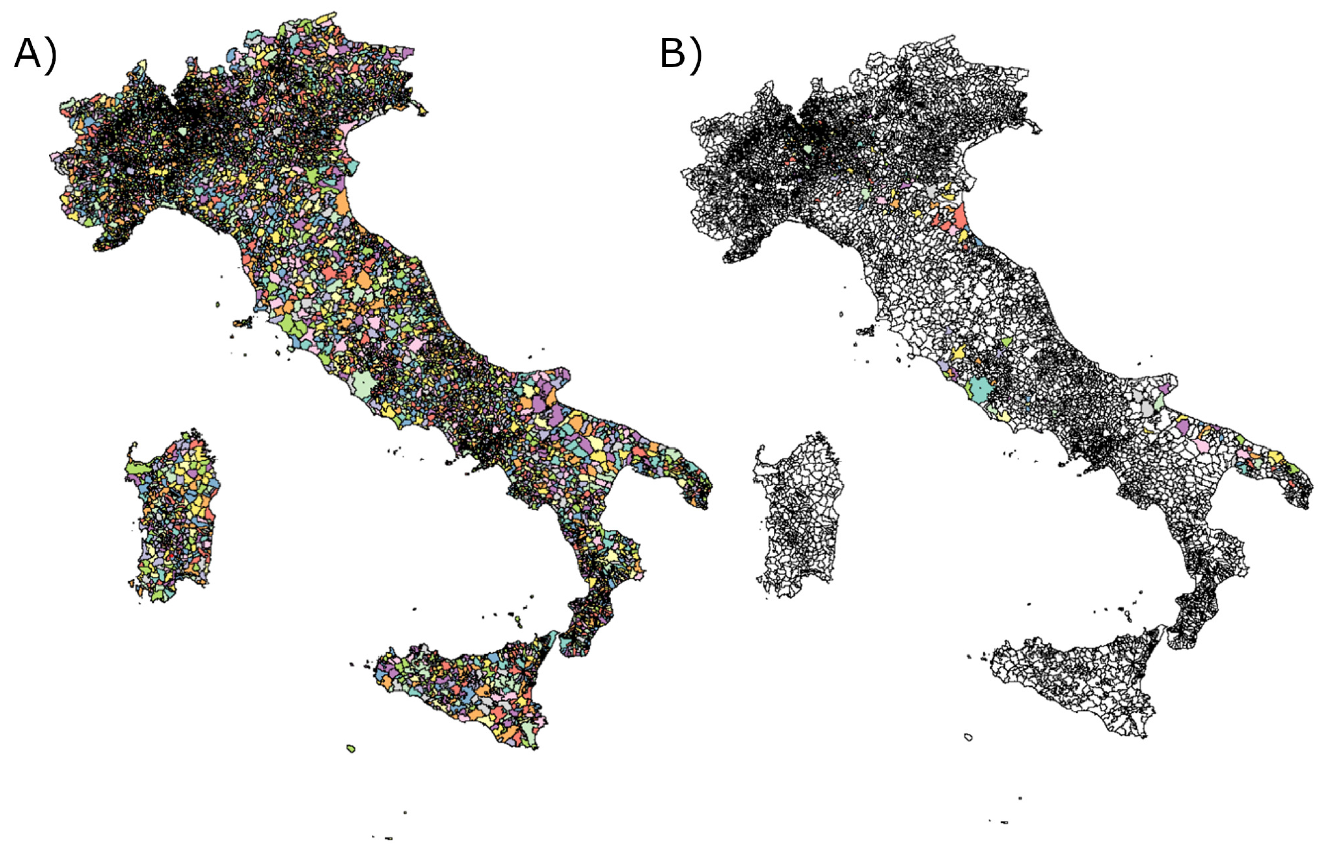
Our work aimed to create a model for estimating the daily ground level concentrations of air pollutants at municipal scale, using satellite, meteorological and geographical data over the period 2019–2022. To this end, we used artificial intelligence techniques for the creation of the model and Explainable Artificial Intelligence (XAI), for the interpretation of the results. The model, based on ensemble algorithms, was trained using data from 337 ARPA control units, distributed over 4 different Italian regions and considered as the ground truth of our framework. Panel A of Figure 1 shows the Italian territory with all the considered municipalities in Italy; panel B displays the control units used in our analysis. Municipal areas range from 1 to 1287.24 km2 with an average of 37.3 km2.
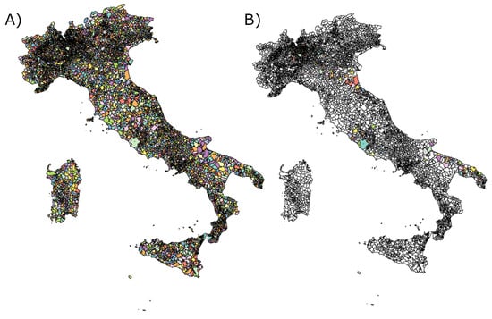
Figure 1.
On the left (panel A) a representation of Italian municipalities (8092), on the right (panel B) a representation of municipalities with at least one ARPA control unit.
We compared our findings with the predictions provided by Copernicus Atmosphere Monitoring Service (CAMS) global reanalysis dataset [7]. CAMS [8] is a service implemented by the European Centre for Medium-Range Weather Forecasts (ECMWF), based on a variety of ground level and satellite retrieved data. Its purpose is to provide continuous information on atmospheric composition including total column values for and and surface concentrations of and .
The proposed model, optimized at the municipal level, could facilitate One Health studies as well as support local and national stakeholders, agencies, and policymakers.
2. Materials and Methods
The goal of our study was to develop a model to estimate ground level air pollution in Italy at the municipal level from 2019 to 2022 through heterogeneous data such as satellite, meteorological, geographical and social data. In particular, we focused on the estimation of ground level concentrations of 4 air pollutants, namely , , and , through a machine learning approach, as summarized in Figure 2. After a preprocessing phase, we selected the ML algorithm with the best performance among linear model, Random Forest and XGBoost, by means of a five-fold cross validation procedure. Then, we implemented a feature importance procedure using an approach based on Shapley (SHAP) values to assess the role of each feature in the model. We collected different types of data for the construction of the machine learning model: satellite, meteorological, and ground pollution data, geographical and social data. All data was preprocessed to have daily time granularity, covering the years between 2019 and 2022 at a municipal scale with a total of 8092 Italian municipalities.
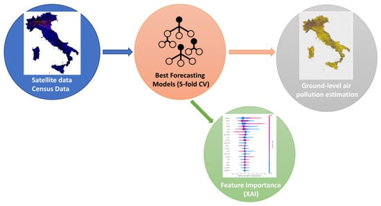
Figure 2.
Flowchart of the analysis. After the collection of satellite, reanalysis and census data we implemented three different models to predict ground-level daily air pollution over all Italian municipalities. Afterwards, we applied a XAI feature importance procedure to understand the role of each feature in the prediction.
2.1. Sentinel-5P Data
Satellite data refers to information collected from Earth-observing satellites orbiting around our planet. These satellites are equipped with various sensors and instruments that capture a wide range of data, including atmospheric composition, meteorological, and environmental parameters. Satellite data has become pivotal for monitoring and understanding Earth’s dynamic processes, climate change, and environmental trends.
Copernicus Sentinel-5P mission is part of the European Space Agency’s Copernicus Earth Observation Program, which aims to provide open and free access to environmental data for a multitude of applications [9]. Sentinel-5P specifically focuses on monitoring the Earth’s atmosphere and plays a crucial role in tracking air quality and atmospheric composition. Sentinel-5P is equipped with a state-of-the-art spectrometer called TROPOMI (Tropospheric Monitoring Instrument). TROPOMI can measure a wide range of atmospheric gases with a spatial resolution of × km2, a swath width of 2600 km and time of overpassing Italy around 2 p.m. It measures a wide range of atmospheric trace gases such as nitrogen dioxide (), ozone (), sulfur dioxide (), and carbon monoxide (), among others. These measurements are crucial to assess air pollution, greenhouse gas levels and to evaluate their impact on climate and human health [10].
For the construction of the model, we collected daily concentrations of pollutants, namely and from the Google Earth Engine [11,12]. From the same source we collected the Aerosols Absorbing Index [13], which can be used to determine the presence of UV-absorbing aerosols, such as dust and smoke. Positive values of this index indicate the presence of these pollutants. This index can be a proxy for the concentration of and and positive values of this index indicate the presence of elevated absorbing aerosols in the Earth’s atmosphere.
The original spatial resolution of this data is × km2, however Google Earth Engine converts original L2 data to L3 images using a grid with the pixel size smaller then the actual resolution in order to avoid data loss. The final spatial resolution is then × km2.
2.2. ERA5 Data
Climate reanalysis data combine past observations collected by a variety of sources on land, ocean, airplains, satellites and from instruments with different lifespans, quality and resolution with models to generate consistent time series of multiple climate variables.
ERA5 stands for the “Fifth Generation European Reanalysis”. It is a project led by ECMWF that aims to create a comprehensive, high-quality dataset of historical and current weather and climate information [14].
ERA5 utilizes a large amount of observational data including data from satellites, weather stations, aircraft, and more, to reconstruct the Earth’s atmospheric conditions and surface variables. This reanalysis dataset provides a consistent and detailed record of past weather and climate conditions on a global scale, allowing scientists and researchers to analyze long-term climate trends, investigate extreme weather events, and improve climate modeling and forecasting.
From the Google Earth Engine we collected ERA5 [15], namely temperature 2 m above ground, surface pressure, u and v component of wind 1 m above the surface and the amount of precipitation. The spatial resolution of this data is × km2 with a daily granularity. Also, from the wind components we calculated wind speed using the classical Euclidean norm.
2.3. ISTAT Data
For a further spatial characterization of the municipalities, we collected social and geographical data from public repositories of the Italian National Institute of Statistics (ISTAT). ISTAT is the primary governmental agency responsible for collecting, analyzing, and disseminating statistical information in Italy [16]. From the ISTAT repository we extracted 39 features from the 2011 census data [17], reported in the Supplementary Materials. Features include altitude, type (coastal, urban, etc…), population density, density of buildings, density of roads and number of workers for each municipality.
2.4. ARPA Ground Data
We used pollution data from ARPA ground stations as labels to train our machine learning model. The environmental quality monitoring conducted by ARPA involves the systematic assessment and measurement of various environmental parameters within individual regions. This monitoring process includes the collection and analysis of data related to air and water quality, soil conditions, noise levels, and other environmental factors.
To train our model, we collected air pollution data from 337 control units located in four regions: Puglia (60 control units) [18], Lazio (53 control units) [19], Emilia Romagna (54 control units) [20] and Lombardy (170 control units) [21], placed in the Southern, Central, Northeastern, and Northwestern part of Italy, respectively. The set of control units has been chosen to be as heterogeneous as possible. The types of stations are: Traffic, Industry and Background. The areas are: Urban, Suburban and Rural. The data are hourly or daily averages, cover the period between 2019 and 2022, and provide concentrations in g/m3 of four pollutants, namely , , and .
We have chosen these 4 regions for a double reason: (i) these regions are representative of the territorial and climatic diversity of Italy due to their geographical location; (ii) to reduce computational costs, since the analysis of these data required in fact several days of processing.
To improve the performance of our framework in estimating ground level concentrations of a pollutant, we also used satellite measurements of the other three pollutants Section 2.1) as independent variables of the model, given the high correlation between the different pollutants (see Figure S1 of the Supplementary Materials).
3. Data Preprocessing
We followed a preprocessing strategy to handle the missing data to reduce redundant information in our dataset and to address data colocation in time and space. Data missingness is an issue inherent to the nature of satellite data, since not all Italian areas are crossed daily by the satellite’s orbit. On the other hand, the ARPA data also contained missing values mainly due to malfunction or temporary shutdowns of the control units. To overcome this problem, we removed all observations with missing ground level data from the control unit. The percentage of missing values in the ARPA data was 1% for , 19% for , 23% for and 3% for .
As for the data obtained by satellite, these variables were downloaded at level L3, i.e., with pixels that have a QA value > . The percentages of missing values were for , for and for AAI. To encode time-related information in the model we added three features, namely year, month and day of the week. With the exception of year, we converted time variables using cyclic encoding from R’s Lubridate package. Cyclic encoding of time variables involves the representation of time data in a circular or periodic manner. Cyclic encoding of time variables is a common practice in machine learning. Through this procedure it is possible to capture recurring patterns within a data set. For example, if an input feature of the model is month of the year, ordinary encoding will match the month with an integer between 0 an 11, starting with January; in this encoding January (0) and December (11) will be very different even though they are close temporally. Generally, periodic functions such as sine and cosine are used to encode time variables such as day of the week and month [22]. This is often referred to as circular coding or circular representation. In our case, we represented the days of the week as if they were angles we then applied the sine and cosine functions:
where d is the day of the week, an integer between 0 and 6 starting from Monday and N is 7. Then we calculated:
We repeated the same procedure to encode the months of the year by replacing d in (1) with an integer between 0 and 11, starting with January, and N with 12. At the end our dataset was composed by 68 features including satellite, meteorological, geografical and social variables.
A first Pearson correlation analysis highlighted a strong correlation between some features. Therefore, to remove the redundant information we selected a correlation threshold of 50% such that no two variables that have a correlation greater this threshold are included in the model which reduced the final number of features to 32. We selected the threshold that minimized the error of the model. In the Supplementary Materials we list all features used in the model, including redundant features.
When the data from the ARPA control units had an hourly time granularity, we averaged over a daily time window to achieve the granularity of satellite data. Our input data also had different spatial granularity. Since our analysis had the granularity of municipalities, when the input data had higher resolution, we averaged measurements covering the same municipality.
The spatial analysis required the use of different R packages. The used packages were gstat, raster, sf and exactextractr. Specifically, the satellite images were downloaded in .tif format from Google Earth Engine and read in with the raster package. The image was then re-projected into the same coordinate reference system (CRS) as the shapefile used for the Italian municipality. Finally, the image values were extracted with the exactextractr package, using the mean value as an aggregation function.
4. Learning Framework
We implemented a learning framework to estimate the daily ground concentration at the municipal level of the following air pollutants: , , and . We started with a linear model, then we compared the performance of this model with two machine learning algorithms: Random Forest and XGBoost. We trained our model with the data collected by 337 control units located in four regions within a 5-fold cross validation (CV) framework, repeated 100 times, to further increase the robustness of our procedure [23]. In this procedure, for a given day, the initial dataset containing data of 337 control units is randomly divided into 5 subsets without re-insertion: 4 subsets represent the training set and the remaining subset is used for validation.
4.1. Linear Model
Multiple linear regression is one of the most widely used statistical models. This model examines the relationship between a dependent variable (y), some independent variables () and their interactions under a linear hypothesis:
where is the intercept value, are the regression coefficients to fit, is the model error and n is the number of features used in the model.
4.2. Random Forest
The Random Forest (RF) [24] model has gained widespread popularity in the field of Machine Learning, particularly in recent years. This algorithm combines the strengths of both decision trees and the bagging strategies. Similarly to decision trees, the model delves deep into the data, assessing the significance of specific variables at each node and branching accordingly. However, the key distinction lies in the simultaneous use of multiple decision trees, each specializing in a random sample drawn from the complete dataset in a bootstrap mode.
The parameter m, representing the number of variables used for training at each node, is a hyperparameter that can be customized by the programmer. Typically, a recommended value for this parameter is , where N stands for the total number of variables. Another parameter that can be configured is the total number of trees of the forest. During the growth of the forest, the value of m remains constant while each tree is expanded to its maximum extent without employing any pruning techniques.
In our analysis we used R package randomForest with a number of trees equal to 500 and [25].
4.3. XGBoost
Extreme Gradient Boosting (XGBoost), represents a highly optimized version of the gradient boosting algorithm with the added advantage of parallelization. Parallelization significantly enhances the speed of the training process [26]. Rather than focusing on training a single optimal model with the entire dataset, XGBoost adopts a different approach. It trains numerous models on various subsets of the training data and subsequently selects the best-performing model through a voting mechanism. In many scenarios, XGBoost outperforms traditional gradient boosting algorithms.
We implemented this model using R package XGBoost, using the default parameters, booster gbtree and 500 runs [27].
4.4. Performance Metrics
To evaluate performances we used the coefficient of determination between predicted and actual values:
the mean absolute percentage error (MAE), defined as:
and the root mean square error (RMSE), defined as:
with that represents the actual value, the predicted value and the mean of the actual values.
5. Explainable Artificial Intelligence and SHAP Values
The SHAP (SHapley Additive exPlanation) technique is a mathematical approach employed to elucidate the predictions generated by a machine learning model [28]. It relies on principles from cooperative game theory to investigate the contribution of each variable in the model’s predictions. In other words, SHAP serves as an individualized model-agnostic interpreter. It operates under the assumption that the model being elucidated is a black box, meaning its internal workings are not known. Therefore, SHAP can only access the input data and the predictions produced by the model. The primary objective of this interpreter is to replicate the entire prediction process of the original model while maintaining interpretability. In our work, we applied the SHAP local explanation method to evaluate the role of each feature in both Random Forest and XGBoost models. We computed the mean SHAP values after a 5-fold CV, repeated 100 times.
The method exploits the concept of the Shapley (SHAP) values. For all possible feature subsets F of the total feature set S () given a feature j the SHAP value is the result of the difference between the output of two models: a first model including the feature, and a second model without that feature. The SHAP value of the j-th feature for the observation x is measured by adding and removing the j-th feature to all possible subsets,
where is the cardinality and all permutation are considered; indicates the model prediction f for obsevation x, considering a subset F without the j-th feature; represents the output of the same model including the j-th feature.
The Shap analysis was performed with Python package shap.
6. Results
6.1. Machine Learning Predictions
In Table 1 we show the performance in terms of Mean Absolute Error (MAE), Root mean Squared Error (RMSE) and obtained using three different models: Linear Model, Random Forest and XGBoost. A 5-fold Cross Validation repeated 100 times was used to obtain the distribution of these metrics. The employed dataset covered the period between 2019 and 2020. The algorithm XGBoost had the best performance.

Table 1.
Results obtained for all pollutants using three different models. The distribution of MAE, RMSE and are obtained using a 5-fold cross validation repeated 100 times.
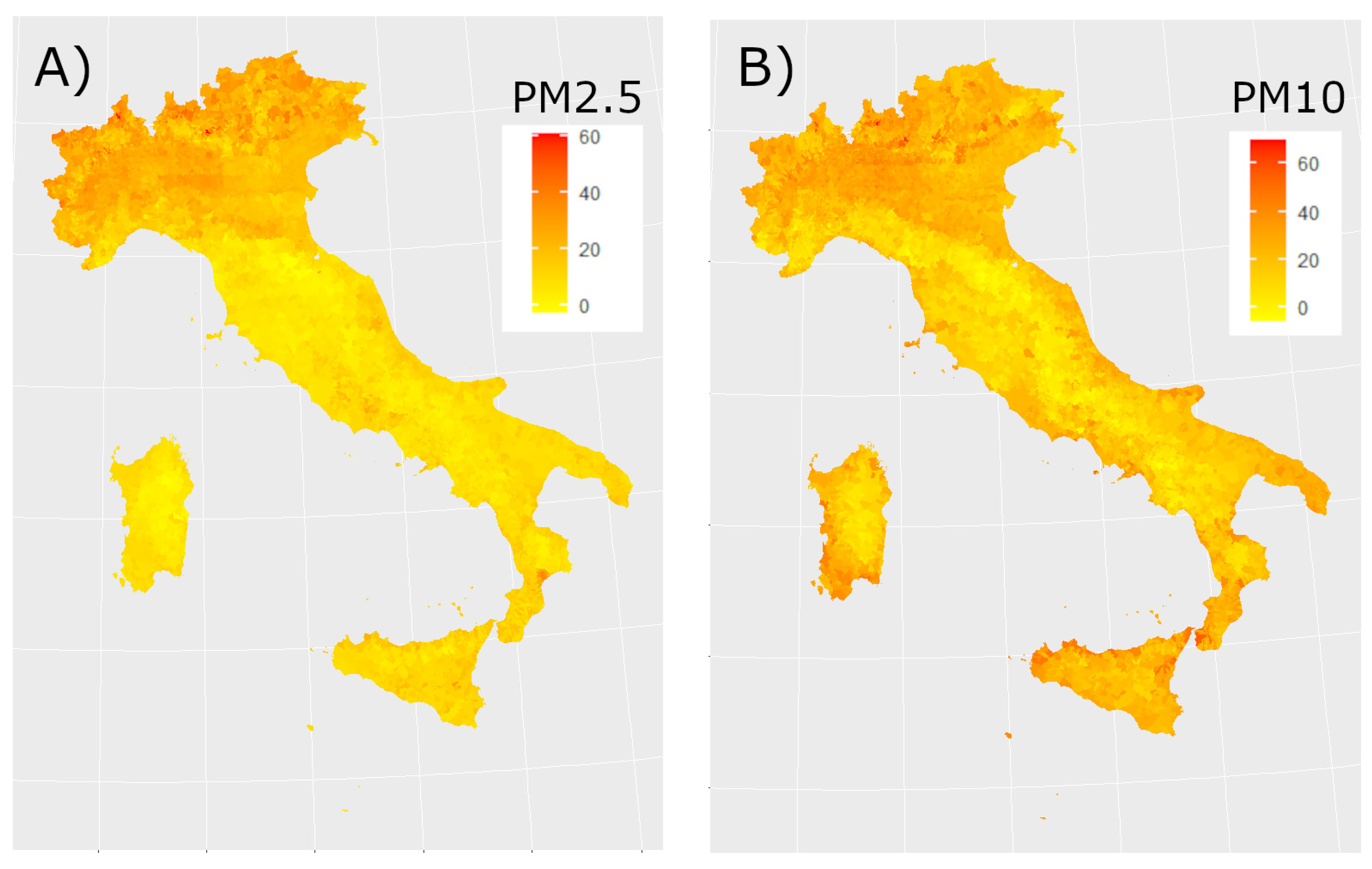
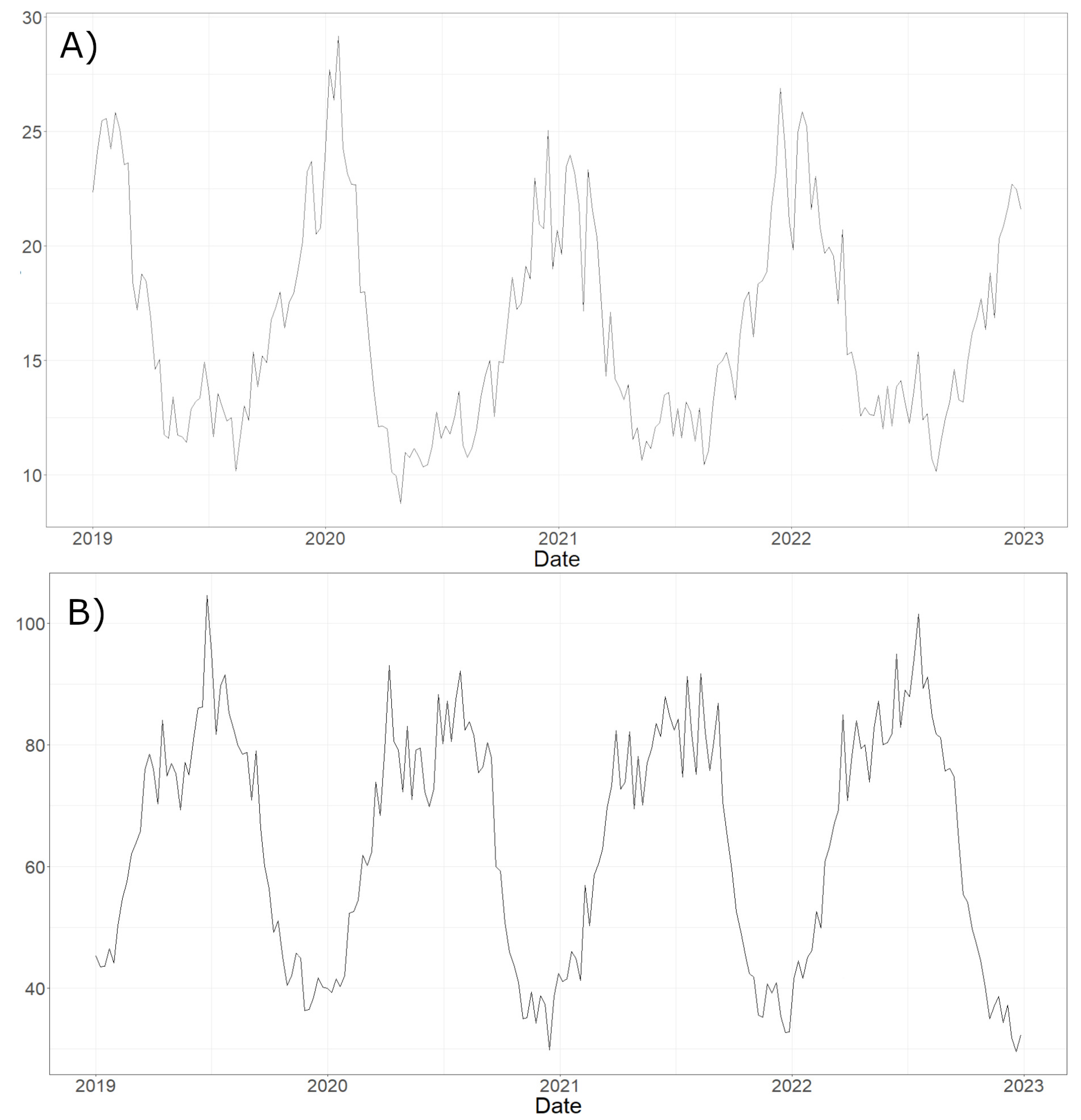
Figure 3 and Figure 4 show the daily maps obtained from the model for all considered pollutants on the same day. Figure 5 displays the time series of estimated concentrations (Panel A) and of estimated concentrations (Panel B) averaged over all Italian municipalities with a time window of 7 days. We can underline that a seasonal behaviour in the concentration of the pollutants is manifest as reported in [29,30,31].
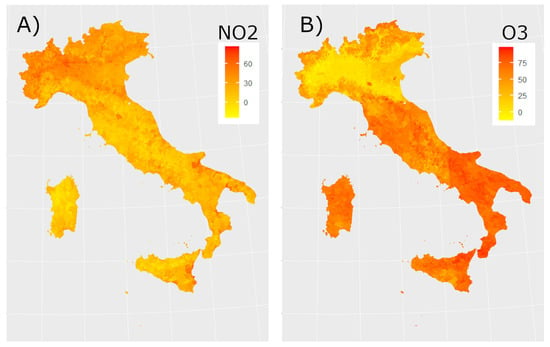
Figure 3.
On the left (panel A) estimated concentrations (g/m3), on the right (panel B) estimated concentrations (g/m3) for date 1 February 2019.
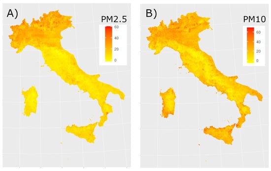
Figure 4.
Left panel (panel A) estimated concentrations (g/m3), on the right panel (panel B) estimated concentrations (g/m3), both on 1 February 2019.
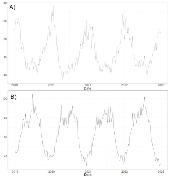
Figure 5.
Time series of concentrations (g/m3) (panel A) estimated by the model, averaged over all Italian municipalities with a time window of 7 days. Below, (panel B) time series of the estimated concentrations (g/m3).
6.2. SHAP Values
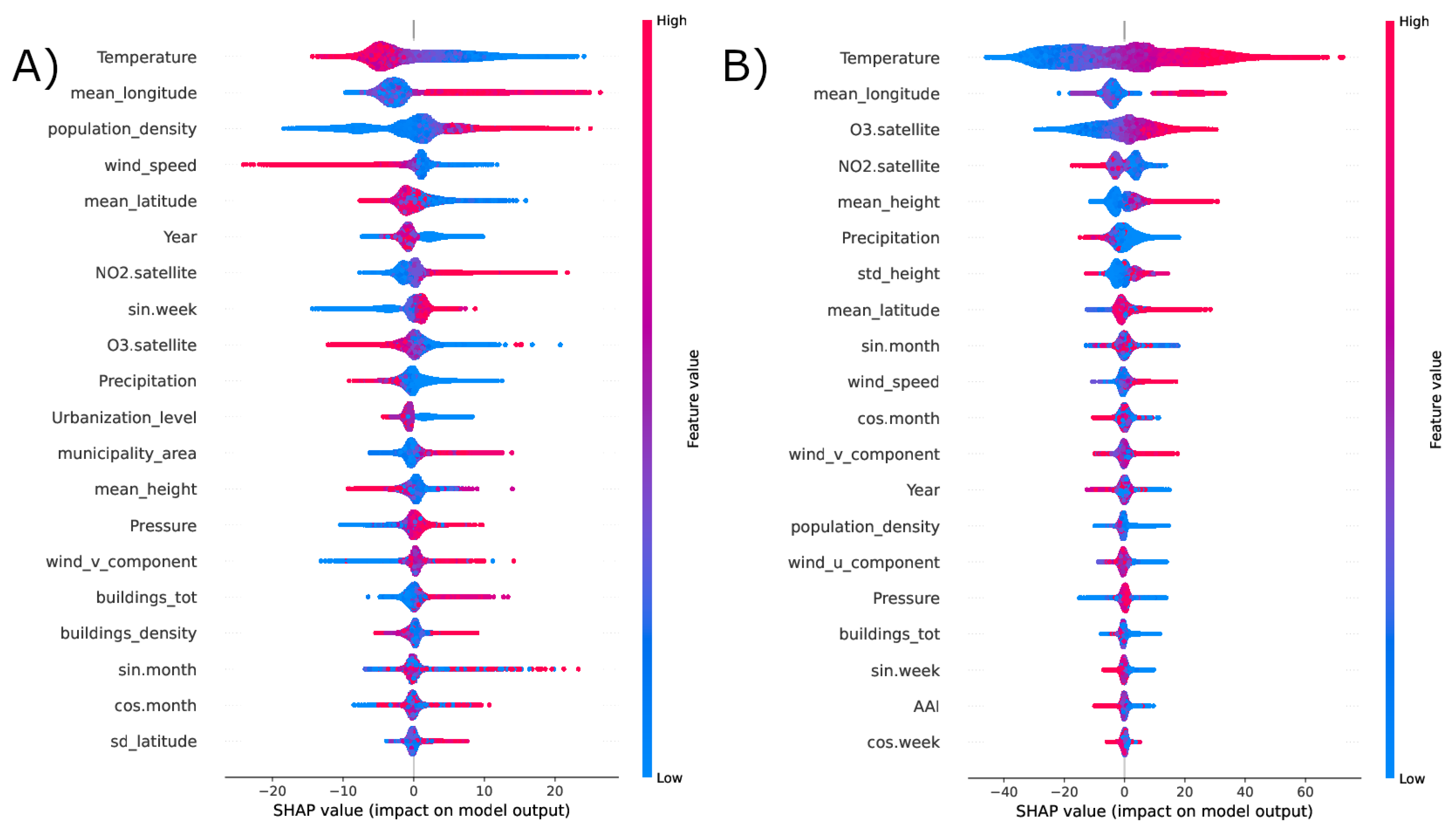
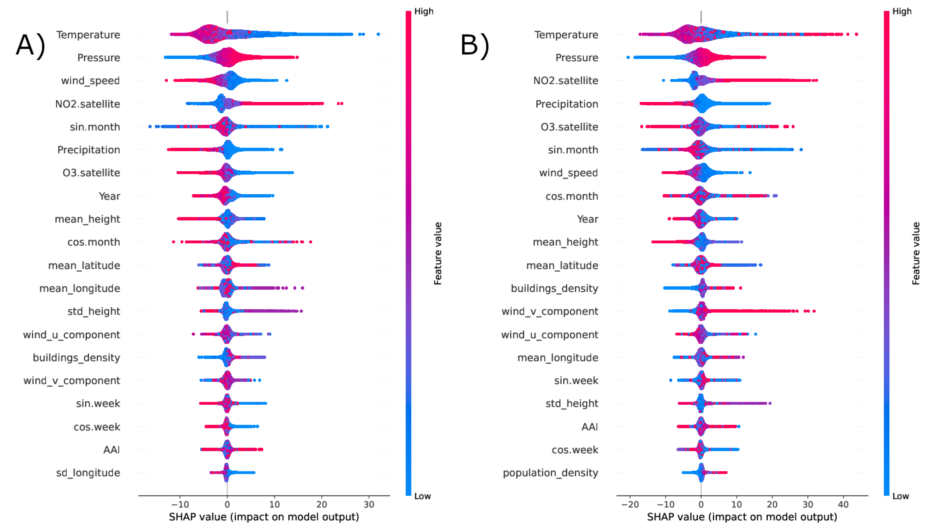
Figure 6 and Figure 7 contain the SHAP plots of the estimation of , , and concentrations, respectively. The distributions are obtained using a repeated cross validation approach. In these plots, on the y axis the relevant features for each pollutants are ordered in terms of the mean absolute SHAP value, which indicates their overall impact on the estimated concentrations. Instead, the x axis indicates how each feature affects the model prediction, e.g., in a positive or negative way (sign of x) and to what extent (x absolute value). Each point corresponds to a prediction, red corresponds to higher values of a feature.
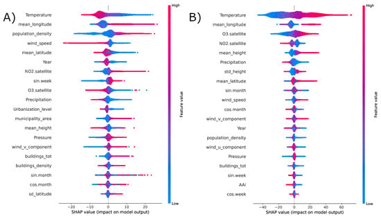
Figure 6.
SHAP values distribution for the prediction of (left, panel A) and (right, panel B) concentrations, obtained in cross validation.
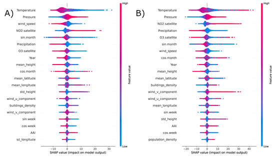
Figure 7.
SHAP values distribution for the prediction of (left, panel A) and (right, panel B) concentrations, obtained using a cross validation.
7. Discussion
Our model aims at estimating daily ground level air pollution in Italian municipalities. Our choice of the granularity, namely at the level of municipality, is motivated both by a reduction of the model complexity and by our intention to use our results in a future One Health study, where only the municipality of residence is known—as it is usually the case in population studies. As we can see from Table 1, XGBoost is the best model for estimating the four pollutants considered. In addition, this model has the highest computational performance. The performance of our model seems comparable, or even superior, to those reported in the literature.
Our results are in line with the literature. Stafoggia, M et al. [32] applied a multilevel approach to obtain daily maps of and in Italy by using the Random Forest algorithm as predictor and Institute for Environmental Protection and Research (ISPRA) monitoring stations as ground truth together with different meteorological, geographical and land use variables. Comparing the errors obtained with a cross validation procedure, we see that the RMSE of their model in predicting is g/m3 in the best case, while our model reaches g/m3; for their error is g/m3, while ours is 5.46 g/m3. It is worth mentioning that the spatial resolution of their estimates is 1 km, which is higher than our model.
Cedeno et al. [33] reported a RMSE value of g/m3 predicting the daily concentration of in the area of Milan and using ARPA’s control units as ground truth and Machine Learning models.
Silibello et al. [34] estimated the daily ground level concentration of and Ozone using the Random Forest algorithm, geographical variables and a model called FARM. Also in this case the spatial resolution of the model was 1 km. The best RMSE values found were and g/m3 for and respectively.
Chen et al. [35] obtained a RMSE of g/m3 for the prediction of surface Ozone in a large area of China, using meteorological data between September 2015 and August 2021. As regards , Chu-Chih Chen et al. [36] presented a machine learning framework to forecast the monthly concentrations of Taiwan at different spatial resolutions obtaining a of , comparable with the results of our XGBoost model. Peddle et al. [37] used Aerosol Optical Depth data to predict concentrations of and for six US urban areas: Los Angeles, CA; Chicago, IL; St. Paul, MN; Baltimore, MD; New York, NY; Winston-Salem, NC. This study covered a period between 2000 and 2012 obtaining a performance in terms of ranging from to .
Figure 5 highlights a seasonal trend of the concentration of and , pollutants that are particularly related to temperature and urban pollution, as shown by Nguyen et al. [29], who also emphasised the relationship between the concentration of and heating systems and population density.
In a study conducted by Di Bernardino et al. [38] in Italy, the same seasonal behaviour of and was found when analyzing control sites in Rome. When analyzing weekly concentrations, they also concluded that the decrease in was related to the decrease in urban traffic that typically accompanies the weekend. Another study in Italy by Ravina et al. [39] confirmed these results. They investigated the concentrations of two stations in the Turin area and showed the influence of temperature on the and concentrations. In particular, by comparing the trends of concentrations measured by two different stations, they found significant differences during the winter season. This behavior seems to be influenced by the increased traffic volume and home heating.
The connection among and concentrations, temperature and population density is confirmed by the results of our SHAP analysis displayed in Figure 6, which shows the twenty features with the highest shap values. As we can see, population density plays a crucial role in predicting on the ground surpassing the influence of satellite retrieved . However, the influence of the urban context seems to be less influential for the prediction of . Nevertheless, the pivotal role of temperature is confirmed, in particular high temperatures are associated with higher values of concentrations and the opposite is true for , which is expected. In fact, is a secondary pollutant whose formation is catalyzed by solar radiation [30]. Satellite measures of and concentrations are anti-correlated with each other and play an important role in predicting ground level concentrations of both and , as expected [40,41].
The Shap diagrams for particulate matters, which are shown in Figure 7, indicate that wind speed plays a decisive role in addition to temperature and appears to be anti-correlated with the model results [42]. The role of the wind in moving the dust masses and reducing their concentrations is straightforward. An interesting result is the importance given by the model to the south-north component (wind_v_component) of the wind, which is positively correlated with particulate concentrations except for perhaps where positive and negative contributions are mixed and could indicate the transport of dust from Africa to the Italian regions.
This result is confirmed by other studies. Calidonna et al. [43] conducted medium-term observations at the GAW regional observatory in Lamezia Terme from 2015–2019 to identify dust outbreaks and investigate aerosol properties. They investigated an intense dust outburst episode in April 2019 as a case study and performed a detailed analysis considering surface and column optical properties, chemical properties, air quality modeling, satellite products and the return trajectory analysis, confirming the role of wind speed as the main cause of dust transportation.
Other meteorological variables that emerge as important in the model are precipitations and pressure; their behaviour confirms the goodness of our model. In particular, from the Shap diagrams we can see that precipitation is negatively correlated with the concentrations of the different pollutants, while pressure is positively correlated. This is a reasonable result, since rain combined with low pressure causes air pollutants to precipitate on the surface and their concentration to decrease [44].
Time-related features also seem to play an important role within the model. For example, in the estimation of concentrations, variable sin.week, which correlates positively with the prediction, could be related to the “weekend effect” [45], which links the concentration of with the traffic flow [46]. The Shap diagrams show that the use of satellite measurements of and in the model to estimate ground level concentrations of the four considered pollutants was important. In contrast, the aerosol absorption index was not among the most important variables for the prediction of and . This result is consistent with the literature. The Aerosol Absorption Index does not in fact provide a quantitative measure of the concentration of aerosols, but is used for special events such as volcanic eruptions, large dust events and forest fires [47].
Finally, as mentioned in the introduction, we compared the results of our model with the predictions of the CAMS model, which are available from 1 July 2021. For the comparison, we used linear correlation because and measurements provided by CAMS have different units of measurement than ground station measurements, namely (kg/m2) versus (kg/m3). Table 2 shows the values of the linear correlations between the values provided by CAMS, the results of our model and the ground truth provided by ARPA. From these values we can see that, unlike our models predictions, CAMS predictions are not statistically correlated with ground station measurements. This low correlation may be due to the granularity of the CAMS model, which has a spatial resolution of × km2 and therefore ground stations that are not as far, compared to CAMS resolution, are assigned the same predicted value by CAMS even if their geographical and meteorological conditions are different.

Table 2.
Correlation among CAMS predictions, Ground truth values (ARPA) and Our model predictions. Except for , the significance level is less than 1%.
8. Conclusions
We compared three different learning models for the daily prediction of concentrations of , , and of Italian municipalities at the surface level. Our framework incorporates information from heterogeneous data such as satellite, meteorological, geographic and social indicators as well as control station measurements provided by the Regional Environmental Protection Agency for the period 2019–2022 that we used as ground truth. The algorithm XGBoost had the best performance with an average of . Our results outperform or are comparable with results reported in other papers in the literature, although some studies present models with a higher resolution than the one used in this study.
Furthermore we evaluated the impact of the different features on the estimation of the concentration of each pollutant through an eXplainable Artificial Intelligence method using SHAP values to improve the interpretability and transparency of our Machine Learning models. The SHAP analysis confirmed some aspects already described in the literature, such as the anti-correlation between wind speed and and dust concentrations, or the positive correlation between temperature and concentrations.
A possible application of our model can be the prediction of extreme air pollution events combining our procedure with the approach of Varotsos et al. [48]. They developed a model to forecast pollution extremes in Athens given changes in the dynamics of pollution and using data from ground stations. Their approach was based on fitting the surface concentration of , and to the Gutenberg-Richter law. In addition, they introduced the concept of natural time as opposed to clock time. This concept is based on the observation that temporal fluctuations in time series can be used to quantify long-term dependencies and to differentiate the type of self-similarity within the series. As a result, they calculated the average waiting time between successive extreme concentrations of these three pollutants.
Moreover, our model can be used in One Health cohort studies to assess the impact of air pollution on human health at the municipal level. Future improvements of this model could increase the spatial resolution going from municipalities to distances of the order of kilometers.
Supplementary Materials
The following supporting information can be downloaded at: https://www.mdpi.com/article/10.3390/rs16071206/s1, Figure S1: Correlation matrix; Table S1: Features table.
Author Contributions
Conceptualization, A.F., A.M. and E.P.; methodology, A.F., A.M., E.P. and R.C.; software, A.F.; validation, A.F., A.M., E.P., R.C. and T.M.; formal analysis, A.F. and A.M.; investigation, A.F., A.M. and E.P.; resources, A.F. and A.M.; data curation, A.F.; writing—original draft preparation, A.F., A.M. and E.P.; writing—review and editing, A.F., A.M., E.P., T.M., L.B., R.C., A.L., M.L.R., S.T., N.A., R.B.; visualization, A.F., A.M., E.P. and T.M.; supervision T.M., N.A., A.M., R.B. All authors have read and agreed to the published version of the manuscript.
Funding
This paper was funded by the European Union—NextGenerationEU within the National Recovery and Resilience Plan (NRRP), Mission 4 Component 2 Investment 1.4—Call for tender No. 3138 of 16 December 2021 of Italian Ministry of University and Research; Award Number: Project code: CN00000013, Concession Decree No. 1031 of 17 February 2022 adopted by the Italian Ministry of University and Research, CUP H93C22000450007, Project title: National Centre for HPC, Big Data and Quantum Computing. This paper was developed within the project funded by Next Generation EU—“GRINS—Growing Resilient, INclusive and Sustainable” project (PE0000018), Spoke 7, National Recovery and Resilience Plan (NRRP)—“PE9-Mission 4, Component C2, Intervention 1.3”. This work was also funded by the Italian Ministry of Enterprises and Made in ITaly (MIMIT) with the “Project CALLIOPE-Casa dell’Innovazione per il One Health” (FSC 2014–2020, CUP E53C22002800001). This work was also supported by the Assessment of PM Exposure at intra-urban scale in preparation of MAIA mission (APEMAIA) project, funded by the Italian Space Agency, CALL FOR IDEAS “ATTIVITÀ SCIENTIFICHE A SUPPORTO DELLO SVILUPPO DELLE MISSIONI DI OSSERVAZIONE DELLA TERRA”, Contract n. 2023-39-HH.0.
Data Availability Statement
All codes and data used to perform the analysis are available upon request.
Conflicts of Interest
The authors declare no conflict of interest.
References
- Kingsley, P.; Taylor, E. One Health: Competing perspectives in an emerging field. Parasitology 2017, 144, 7–14. [Google Scholar] [CrossRef] [PubMed]
- Martin, R.V. Satellite remote sensing of surface air quality. Atmos. Environ. 2008, 42, 7823–7843. [Google Scholar] [CrossRef]
- Fadadu, R.P.; Balmes, J.R.; Holm, S.M. Differences in the estimation of wildfire-associated air pollution by satellite mapping of smoke plumes and ground-level monitoring. Int. J. Environ. Res. Public Health 2020, 17, 8164. [Google Scholar] [CrossRef] [PubMed]
- Veefkind, J.P.; Aben, I.; McMullan, K.; Förster, H.; De Vries, J.; Otter, G.; Claas, J.; Eskes, H.; De Haan, J.; Kleipool, Q.; et al. TROPOMI on the ESA Sentinel-5 Precursor: A GMES mission for global observations of the atmospheric composition for climate, air quality and ozone layer applications. Remote Sens. Environ. 2012, 120, 70–83. [Google Scholar] [CrossRef]
- Li, C.; Liu, M.; Hu, Y.; Wang, H.; Xiong, Z.; Wu, W.; Liu, C.; Zhang, C.; Du, Y. Investigating the vertical distribution patterns of urban air pollution based on unmanned aerial vehicle gradient monitoring. Sustain. Cities Soc. 2022, 86, 104144. [Google Scholar] [CrossRef]
- Maranzano, P. Air quality in Lombardy, Italy: An overview of the environmental monitoring system of ARPA Lombardia. Earth 2022, 3, 172–203. [Google Scholar] [CrossRef]
- Peuch, V.H.; Engelen, R.; Rixen, M.; Dee, D.; Flemming, J.; Suttie, M.; Ades, M.; Agustí-Panareda, A.; Ananasso, C.; Andersson, E.; et al. The copernicus atmosphere monitoring service: From research to operations. Bull. Am. Meteorol. Soc. 2022, 103, E2650–E2668. [Google Scholar] [CrossRef]
- Peuch, V.H.; Engelen, R.; Ades, M.; Barré, J.; Inness, A.; Flemming, J.; Kipling, Z.; Agusti-Panareda, A.; Parrington, M.; Ribas, R.; et al. The use of satellite data in the Copernicus Atmosphere Monitoring Service (CAMS). In Proceedings of the IGARSS 2018-2018 IEEE International Geoscience and Remote Sensing Symposium, Valencia, Spain, 22–27 July 2018; pp. 1594–1596. [Google Scholar]
- Sentinel-5P. 2023. Available online: https://sentinels.copernicus.eu/web/sentinel/missions/sentinel-5p (accessed on 19 December 2023).
- Wei, F. Advance of Study on The Impact of Air Pollution on Human Health. WORLD SCI-TECH R D 2000, 3, 14–18. [Google Scholar]
- NO2 Data. Available online: https://developers.google.com/earth-engine/datasets/catalog/COPERNICUS_S5P_OFFL_L3_NO2 (accessed on 14 October 2023).
- O3 Data. Available online: https://developers.google.com/earth-engine/datasets/catalog/COPERNICUS_S5P_OFFL_L3_O3 (accessed on 15 October 2023).
- AAI Data. Available online: https://developers.google.com/earth-engine/datasets/catalog/COPERNICUS_S5P_OFFL_L3_AER_AI (accessed on 11 October 2023).
- Hersbach, H.; Bell, B.; Berrisford, P.; Hirahara, S.; Horányi, A.; Muñoz-Sabater, J.; Nicolas, J.; Peubey, C.; Radu, R.; Schepers, D.; et al. The ERA5 global reanalysis. Q. J. R. Meteorol. Soc. 2020, 146, 1999–2049. [Google Scholar] [CrossRef]
- ERA5 Data. Available online: https://developers.google.com/earth-engine/datasets/catalog/ECMWF_ERA5_DAILY (accessed on 10 November 2023).
- ISTAT. Available online: https://www.istat.it/ (accessed on 30 September 2023).
- ISTAT Data. Available online: http://dati.istat.it/ (accessed on 30 September 2023).
- ARPA Data—Puglia Region. Available online: http://old.arpa.puglia.it/web/guest/meta-aria (accessed on 1 December 2023).
- ARPA Data—Lazio Region. Available online: https://www.arpalazio.net/main/aria/sci/basedati/chimici/chimici.php (accessed on 4 December 2023).
- ARPA Data—Emilia Romagna Region. Available online: https://arpaeprv.datamb.it/dataset/qualita-dell-aria-rete-di-monitoraggio/resource/7efd47bc-31e3-4f7d-bca4-e1b01f80a304 (accessed on 23 November 2023).
- ARPA Data—Lombardy Region. Available online: https://www.dati.lombardia.it/stories/s/auv9-c2sj (accessed on 23 November 2023).
- Tateo, A.; Campanaro, V.; Amoroso, N.; Bellantuono, L.; Monaco, A.; Pantaleo, E.; Rinaldi, R.; Maggipinto, T. TPredicting Air Quality from Measured and Forecast Meteorological Data: A Case Study in Southern Italy. Atmosphere 2023, 14, 475. [Google Scholar] [CrossRef]
- Browne, M.W. Cross-Validation Methods. J. Math. Psychol. 2000, 44, 108–132. [Google Scholar] [CrossRef] [PubMed]
- Breiman, L. Random forests. Mach. Learn. 2001, 45, 5–32. [Google Scholar] [CrossRef]
- randomForest Documentation. Available online: https://www.rdocumentation.org/packages/randomForest/versions/4.7-1.1/topics/randomForest (accessed on 3 November 2023).
- Chen, T.; Guestrin, C. Xgboost: A scalable tree boosting system. In Proceedings of the 22nd ACM Sigkdd International Conference on Knowledge Discovery and Data Mining, San Francisco, CA, USA, 13–17 August 2016; pp. 785–794. [Google Scholar]
- XGboost Documentation. Available online: https://xgboost.readthedocs.io/en/stable/parameter.html (accessed on 3 November 2023).
- Ribeiro, M.T.; Singh, S.; Guestrin, C. “Why should i trust you?” Explaining the predictions of any classifier. In Proceedings of the 22nd ACM SIGKDD International Conference on Knowledge Discovery and Data Mining, San Francisco, CA, USA, 13–17 August 2016; pp. 1135–1144. [Google Scholar]
- Nguyen, H.T.; Kim, K.H.; Park, C. Long-term trend of NO2 in major urban areas of Korea and possible consequences for health. Atmos. Environ. 2015, 106, 347–357. [Google Scholar] [CrossRef]
- Wang, Y.; Shim, C.; Blake, N.; Blake, D.; Choi, Y.; Ridley, B.; Dibb, J.; Wimmers, A.; Moody, J.; Flocke, F.; et al. Intercontinental transport of pollution manifested in the variability and seasonal trend of springtime O3 at northern middle and high latitudes. J. Geophys. Res. Atmos. 2003, 108, ACH11-1–ACH11-11. [Google Scholar] [CrossRef]
- Lai, S.C.; Zou, S.C.; Cao, J.J.; Lee, S.C.; Ho, K.F. Characterizing ionic species in PM2.5 and PM10 in four Pearl River Delta cities, South China. J. Environ. Sci. 2007, 19, 939–947. [Google Scholar] [CrossRef] [PubMed]
- Stafoggia, M.; Bellander, T.; Bucci, S.; Davoli, M.; De Hoogh, K.; De’Donato, F.; Gariazzo, C.; Lyapustin, A.; Michelozzi, P.; Renzi, M.; et al. Estimation of daily PM10 and PM2. 5 concentrations in Italy, 2013–2015, using a spatiotemporal land-use random-forest model. Environ. Int. 2019, 124, 170–179. [Google Scholar] [CrossRef] [PubMed]
- Cedeno Jimenez, J.R.; Pugliese Viloria, A.d.J.; Brovelli, M.A. Estimating Daily NO2 Ground Level Concentrations Using Sentinel-5P and Ground Sensor Meteorological Measurements. ISPRS Int. J. Geo-Inf. 2023, 12, 107. [Google Scholar] [CrossRef]
- Silibello, C.; Carlino, G.; Stafoggia, M.; Gariazzo, C.; Finardi, S.; Pepe, N.; Radice, P.; Forastiere, F.; Viegi, G. Spatial-temporal prediction of ambient nitrogen dioxide and ozone levels over Italy using a Random Forest model for population exposure assessment. Air Qual. Atmos. Health 2021, 14, 817–829. [Google Scholar] [CrossRef]
- Chen, B.; Wang, Y.; Huang, J.; Zhao, L.; Chen, R.; Song, Z.; Hu, J. Estimation of near-surface ozone concentration and analysis of main weather situation in China based on machine learning model and Himawari-8 TOAR data. Sci. Total Environ. 2023, 864, 160928. [Google Scholar] [CrossRef]
- Chen, C.C.; Wang, Y.R.; Yeh, H.Y.; Lin, T.H.; Huang, C.S.; Wu, C.F. Estimating monthly PM2. 5 concentrations from satellite remote sensing data, meteorological variables, and land use data using ensemble statistical modeling and a random forest approach. Environ. Pollut. 2021, 291, 118159. [Google Scholar] [CrossRef]
- Pedde, M.; Kloog, I.; Szpiro, A.; Dorman, M.; Larson, T.V.; Adar, S.D. Estimating long-term PM10-2.5 concentrations in six US cities using satellite-based aerosol optical depth data. Atmos. Environ. 2022, 272, 118945. [Google Scholar] [CrossRef]
- Di Bernardino, A.; Mevi, G.; Iannarelli, A.M.; Falasca, S.; Cede, A.; Tiefengraber, M.; Casadio, S. Temporal Variation of NO2 and O3 in Rome (Italy) from Pandora and In Situ Measurements. Atmosphere 2023, 14, 594. [Google Scholar] [CrossRef]
- Ravina, M.; Caramitti, G.; Panepinto, D.; Zanetti, M. Air quality and photochemical reactions: Analysis of NOx and NO2 concentrations in the urban area of Turin, Italy. Air Qual. Atmos. Health 2022, 15, 541–558. [Google Scholar] [CrossRef] [PubMed]
- Wang, Z.; Lv, J.; Tan, Y.; Guo, M.; Gu, Y.; Xu, S.; Zhou, Y. Temporospatial variations and Spearman correlation analysis of ozone concentrations to nitrogen dioxide, sulfur dioxide, particulate matters and carbon monoxide in ambient air, China. Atmos. Pollut. Res. 2019, 10, 1203–1210. [Google Scholar] [CrossRef]
- Sandhiya, L.; Kolandaivel, P.; Senthilkumar, K. Depletion of atmospheric ozone by nitrogen dioxide: A bifurcated reaction pathway. Theor. Chem. Accounts 2013, 132, 1382. [Google Scholar] [CrossRef]
- Jones, A.M.; Harrison, R.M.; Baker, J. The wind speed dependence of the concentrations of airborne particulate matter and NOx. Atmos. Environ. 2010, 44, 1682–1690. [Google Scholar] [CrossRef]
- Calidonna, C.R.; Avolio, E.; Gullì, D.; Ammoscato, I.; De Pino, M.; Donateo, A.; Lo Feudo, T. Five years of dust episodes at the Southern Italy GAW Regional Coastal Mediterranean Observatory: Multisensors and modeling analysis. Atmosphere 2020, 11, 456. [Google Scholar] [CrossRef]
- Kayes, I.; Shahriar, S.A.; Hasan, K.; Akhter, M.; Kabir, M.; Salam, M. The relationships between meteorological parameters and air pollutants in an urban environment. Glob. J. Environ. Sci. Manag. 2019, 5, 265–278. [Google Scholar]
- Bucsela, E.; Wenig, M.; Celarier, E.; Gleason, J. The “weekend effect” in tropospheric NO2 seen from the Ozone Monitoring Instrument. In Proceedings of the AGU Fall Meeting Abstracts, San Francisco, CA, USA, 10–14 December 2007; Volume 2007, p. A21A-0019. [Google Scholar]
- Carslaw, D.C. Evidence of an increasing NO2/NOx emissions ratio from road traffic emissions. Atmos. Environ. 2005, 39, 4793–4802. [Google Scholar] [CrossRef]
- Prospero, J.M. Long-range transport of mineral dust in the global atmosphere: Impact of African dust on the environment of the southeastern United States. Proc. Natl. Acad. Sci. USA 1999, 96, 3396–3403. [Google Scholar] [CrossRef]
- Varotsos, C.A.; Mazei, Y.; Saldaev, D.; Efstathiou, M.; Voronova, T.; Xue, Y. Nowcasting of air pollution episodes in megacities: A case study for Athens, Greece. Atmos. Pollut. Res. 2021, 12, 101099. [Google Scholar] [CrossRef]
Disclaimer/Publisher’s Note: The statements, opinions and data contained in all publications are solely those of the individual author(s) and contributor(s) and not of MDPI and/or the editor(s). MDPI and/or the editor(s) disclaim responsibility for any injury to people or property resulting from any ideas, methods, instructions or products referred to in the content. |
© 2024 by the authors. Licensee MDPI, Basel, Switzerland. This article is an open access article distributed under the terms and conditions of the Creative Commons Attribution (CC BY) license (https://creativecommons.org/licenses/by/4.0/).

