Abstract
Underwater signal processing is primarily based on sound waves because of the unique properties of water. However, the slow speed and limited bandwidth of sound introduce numerous challenges, including pronounced time-varying characteristics and significant multipath effects. This paper explores a channel estimation method utilizing superimposed training sequences. Compared with conventional schemes, this method offers higher spectral efficiency and better adaptability to time-varying channels owing to its temporal traversal. To ensure success in this scheme, it is crucial to obtain time-varying channel estimation and data detection at low SNRs given that superimposed training sequences consume power resources. To achieve this goal, we initially employ coarse channel estimation utilizing superimposed training sequences. Subsequently, we employ approximate message passing algorithms based on the estimated channels for data detection, followed by iterative channel estimation and equalization based on estimated symbols. We devise an approximate message passing channel estimation method grounded on a Gaussian mixture model and refine its hyperparameters through the expectation maximization algorithm. Then, we refine the channel information based on time correlation by employing an autoregressive hidden Markov model. Lastly, we perform numerical simulations of communication systems by utilizing a time-varying channel toolbox to simulate time-varying channels, and we validate the feasibility of the proposed communication system using experimental field data.
1. Introduction
With the development of information technology, wireless communication technology is no longer limited to the terrestrial. While information technology now extends from terrestrial to aerial spaces to facilitate novel user services, underwater wireless communications (UWC), unfortunately, have been neglected [1]. The main limitation to space–air–ground–ocean (SAGO) information transmission is the UWC technology. However, increasing ocean exploration and development have created a rising need for reliable high-speed underwater acoustic communication [2]. The speed of sound waves in water, approximately 1500 m/s, results in a considerable multipath delay in underwater acoustic channels, which is coupled with a narrow coherence bandwidth. Consequently, despite the relatively narrow acoustic signal bandwidth, the effective bandwidth utilized far exceeds the coherence bandwidth. Hence, an underwater acoustic communication (UAC) system behaves as an ultra-wideband system and is significantly impacted by multipath channels [3,4].The slow speed of sound under water also results in a short correlation time for the underwater acoustic channel compared to the signal duration. Consequently, during underwater acoustic signal processing, the model must account for the channel’s time-varying nature.
Channel estimation and equalization essentially involve linear regression. Research on underwater acoustic channels is crucial for sonar imaging systems. In UACs, underwater communications channels introduce multipath interference, leading to inter-symbol interference. In sonar imaging, this manifests as ghosts [5,6]. Initially, these problems were primarily addressed using algorithms like least squares and recursive least squares. However, as signal processing tools advanced, there was a transition from basic probability methods to Bayesian techniques. This shift emphasized leveraging signal probability and distribution (statistical laws) for estimation purposes, leading to the development of methods such as maximum likelihood estimation, Bayesian estimation, and maximum a posteriori estimation [7]. Approaching the channel estimation and equalization problem from a probabilistic standpoint, methods can be categorized into two main groups: sparse Bayesian learning methods and maximum a posteriori probability estimation. Both types of algorithms are essentially empirical Bayesian algorithms. They marginalize the prior and conditional probability distributions of the signal to approximate the distribution we wish to estimate. Subsequently, they find the optimal solution or its conditional mean from this distribution using the maximum a posteriori probability criterion. Calculating the posterior probability solution precisely is often challenging. Researchers have found that many real signals exhibit sparsity. Leveraging this assumption of sparsity greatly simplifies the process. This approach is exemplified by the expectation propagation (EP) algorithm and numerous approximate message passing (AMP) algorithms [8]. The EP algorithm evolved from the assumed-density filtering (ADF) algorithm [9] and enhances performance through added iterations. Its core principle involves constructing an exponential family of functions and approximating this family and the distribution of signals to be estimated by minimizing KL divergence. This approximation aligns with the assumptions of sparsity and the central limit theorem, which render most signals as Gaussian distributed, thus meeting the assumptions of the exponential family. The AMP algorithms are primarily derived from the belief propagation (BP) algorithm, which is rooted in the sum–product algorithm. BP achieves the solution of the signal’s marginal distribution by representing it as a factor graph and iteratively exchanging information between factor nodes and variable nodes. The BP algorithm exhibits high computational complexity and limited adaptability. As a result, Donoho proposed the AMP algorithm [10], which shares significant similarities with the iterative shrinkage threshold algorithm (ISTA) regarding its form and the Onsager term [11]. Despite this resemblance, AMP’s derivation process relies on message passing algorithm approximation: hence, it is named the approximate message passing algorithm.
Despite advancements, approximate message passing algorithms still have several limitations. Consequently, numerous new algorithms have emerged in recent years to address these issues. Among them, GAMP [12] stands out as a more representative approach that not only advances approximate message passing but also generalizes the model. GAMP combines several earlier methods and achieves efficient computation and systematic approximation of loopy belief propagation (LBP) using the maximal sum algorithm and the sum–product algorithm. Additionally, VAMP [13] and OAMP [14] were proposed by different scholars at nearly the same time. These algorithms primarily address cases involving dictionary matrix pathology or the non-zero mean. By iterating the noise variance and denoising function in approximate message passing algorithms, they remain effective even in less pathological cases. Subsequently, CAMP [15], MAMP [16], UAMP [17], and other algorithms have been proposed.
Utilizing the empirical Bayesian method for channel estimation requires critical establishment of the channel model. Additionally, the time-varying nature of the underwater acoustic channel creates significant disparity between general time-invariant models and convolutional channels for accurately depicting the channel: both in simulation experiments and practical scenarios. The non-Gaussian nature of the underwater acoustic channel is a significant topic in acoustic channel research. The commonly used models include stable- distribution and Gaussian mixture models (GMM). However, using these channel distributions in signal processing presents challenges. For stable- distributions, it is very difficult to obtain the joint distribution because it has no fixed expression, and the statistical parameters can only be approximated by some numerical computation methods. The Gaussian mixture distribution presents challenges in parameter estimation due to its composition of multiple Gaussian distributions. Additionally, the time variation of the underwater acoustic channel is not random, and the autoregressive hidden Markov model (AR-HMM) is the more widely used model to describe this variation. Impulse noise is also an important characteristic of underwater acoustic channels. We explored the application of norm constraints for channel estimation under such noise conditions and observed that a method based on norm constraints effectively suppresses impulse noise [18].
Research on time-varying channels traces back to 1963, when Bello discussed the symmetry of channels in time and frequency [19]. In 2011, Qarabaqi released a simulation toolkit for simulating underwater acoustic time-varying channels on his homepage [20]; however, no channel estimation or equalization methods for time-varying channels were provided. Some scholars adopt adaptive modulation to combat the impact of time-varying factors in underwater acoustic communication [21,22,23,24]. In 2009, Guo et al. introduced a two-way iterative channel estimation method utilizing the AR-HMM model. This method leverages the correlation between the front and back of the channel and integrates it with the Gaussian message passing algorithm [25]. Over the last two years, Yang et al. have integrated the superposition training technique with experimental data to further validate the applicability of this model in UACs [26,27]. Zhang and Rao introduced a temporal-correlation-based T-MSBL algorithm for the AR-HMM model in their paper [28]. However, it primarily addresses the block sparsity problem and is effective only at high SNRs and for channels with strong correlation. The scheme is more suitable for scenarios where MIMO diversity gain is insignificant, indicating the presence of strongly correlated co-channel interference [29]. Currently, minimal research has focused on time-varying channel models and their channel estimation and equalization. In [30], we proposed a TC-AMP algorithm for time-varying channels; it uses a two-layer iterative algorithm to improve the performance of channel equalization. In this paper, we further employ the superimposed training sequence strategy and GMM-distribution-based assumptions.
Investigating the time-varying characteristics of underwater acoustic channels reveals significant challenges in obtaining a dictionary matrix that accurately aligns with both observed signals and those intended for detection. Superposition pilots, also known as implied training sequences, offer a promising solution to the challenge of matching channels and data. Several scholars have already conducted research in this area [31]. Unlike traditional training sequences, this method traverses the training sequence over time. When integrated with message passing algorithms, it facilitates better information iteration across a wider operational spectrum. However, time traversal also entails power loss, necessitating a higher SNR for this method. Time traversal incurs power loss, necessitating higher signal-to-noise ratio requirements for this method. However, it offers unparalleled advantages for time-varying channels, as discussed in references [26,27], which advocate for the superposition of training sequences. Yuan et al. also proposed a communication method based on a superposition pilot to enhance spectrum utilization in communication systems [32]. Despite limited research on combining frequency guide superposition with time-varying models and message passing algorithms, the field of UAC using time-varying channels offers ample opportunities for exploration.
This paper employs superimposed training sequences, where short cyclic sequences are added to the data sequences. The cyclic nature of these short sequences allows for power loss compensation through stacking. Moreover, traversing the training sequences in the time domain helps to better mitigate the mismatch between observations and measurements, thereby enhancing the system’s capability to address time-varying channels. To enhance equalization algorithm performance and channel estimation accuracy, we assume a Gaussian mixture model for the signal. Based on this assumption, we propose iterative equalization and time-varying channel estimation algorithms that employ approximate message passing. The GMM distribution information is updated by the EM algorithm. Feasibility is verified through outfield experiments. Moreover, outfield experiments demonstrate the efficiency of channel estimation and equalization using superimposed frequency guides. This study underscores the significant potential of combining superimposed training sequences with soft iterative channel estimation and equalization algorithms for UACs.
- We propose a communication scheme that uses coarse channel estimation based on superimposed training, AMP equalization, and EM-GMM-AMP channel estimation. Based on the factor graph of the underwater acoustic channel model, an approximate message passing underwater acoustic channel estimation method based on Gaussian mixture distribution is derived.
- We combine the EM-GMM-AMP algorithm with the AR-HMM model for CSI updating based on time correlation, further improving the accuracy of channel estimation.
- The effectiveness of the algorithm proposed in this paper is verified through pool experiments and field experiments.
The paper’s structure is as follows: Section 2 outlines the system model, including the matrix-based representation of time-varying channels and superimposed training sequences. In Section 3, we outline the algorithm derivation, which includes AMP equalization for QPSK signals, AMP channel estimation using the GMM approximation, and updates of forward–backward channel information with AR-HMM. Section 4 presents simulations and outfield experimental validations of the algorithms. Section 5 concludes the paper.
2. System Model
2.1. Time-Varying Channel System Model
The fundamental model employed in this paper is a linear model of the channel: specifically, the convolutional channel, which is denoted as Equation (1) for time-invariant systems.
To simplify, we can represent it in matrix form.
where is the Toeplitz matrix with respect to the channel, which can be expressed as:
The discrete convolution relation can be represented in matrix form. It is important to note that the channel in the equation above is time-invariant. To capture the channel’s time-varying nature, we represent the signal in segments, as depicted in the following figure.
To facilitate the representation, we only selected three segments of the signal for a simple illustration. Signals correspond to the channels , respectively, and in these three segments, the signal within the channel is kept constant in each segment. The segments’ Toeplitz matrices are , and , respectively. Then, the received signals can be obtained . In practical communication systems, there exists a time delay difference among the three signals that corresponds to the length of each signal.
Assuming equal segment lengths, the received signal under the time-varying channel results from the shifted superposition of these segments. For clarity, we denote the length of each signal segment as , the total signal length as , and the channel length as . This approach allows us to express the received signal under time-varying conditions in matrix notation.
where , ,, is a column vector or blanking matrix used to complement the length of the signal. The form of Equation (4) is in perfect agreement with Figure 1, and for more intuition, we can rewrite Equation (4):
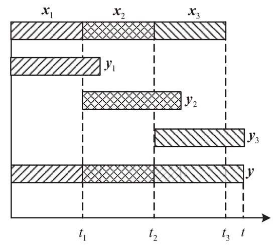
It is worth noting that the dimensions of , , and in the above equation are not necessarily the same; we assume that the length of each segment of the signal is , corresponding to a channel length of ,then, we can get . As we can see in Figure 1, the total length of the signals depends only on the length of the channel corresponding to the last segment of the signal. If we take the limit case where the channel changes for each symbol, we can rewrite the above equation as Equation (6).
where we define this class of Toeplitz matrices as our channel matrix . The above is the model we use in this paper, and in practice, we use a similar approach to Equation (5) in the practical treatment. We provide a specific analysis of the specific superimposed training sequence symbols below.
2.2. Superimposed Training Model
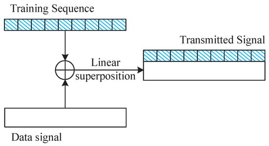
Signal processing involves linearly superimposing QPSK mapped training sequences and source code, as illustrated in Figure 2, to create the base signal for transmission. This enables the real-time estimation of signals in order to acquire the time-varying channel state information matrix essential for this study.
Assuming that our data sequence is , the training sequence is , and to better adapt to time-varying channels, we rewrite the received signal as:
where is the QPSK signal mapped from a binary sequence , is composed of a cyclic sequence , and is Gaussian white noise. Combined with the previously mentioned time-varying channel model, we can represent the time-varying underwater acoustic channel model based on the superimposed training sequences as:
where the channel matrix is a matrix consisting of Toeplitz matrices on the diagonal, and each matrix is defined as:
In conclusion, we have derived the signal representation based on the time-varying channels and superimposed training sequences proposed in this paper.
2.3. Soft Iteration UAC Receiver
Based on the above system model, we have obtained the overall system diagram as shown in Figure 3.
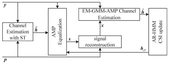
From Figure 3, we can see that first we use the received signal and superimposed training sequence for coarse channel estimation, and then we perform AMP equalization based on the results of the coarse estimation. Channel reconstruction is done using the equalization result, and the reconstructed signal is utilized for channel estimation using the EM-GMM-AMP algorithm. Then, channel information based on AR-HMM is updated based on the results of different estimated blocks and the correlation coefficient of the channel. Based on the updated channel information, the algorithm enters the next equalization cycle. Next, in the third part of this article, we will provide a detailed description of the algorithms used in each part of the system.
3. Channel Estimation and Equalization Based on Superimposed Training Sequences
To initiate the equalization algorithm based on channel estimation, an initial time-varying channel state information matrix must be obtained. This can be achieved relatively easily by incorporating superimposed training sequences. However, due to signal interference and the uncertainty of the time-varying speed, the accuracy of this method may be compromised. Therefore, to enhance accuracy, factor graphs and message passing algorithms are combined in subsequent steps. The proposed time-varying UAC algorithm is based on superimposed training sequences and comprises three main components: coarse channel estimation, an approximate message passing equalization algorithm, and an iterative channel estimation and equalization algorithm based on message passing.
3.1. Coarse Channel Estimation Based on Superimposed Training Sequences
Initially, coarse estimation of the channel is conducted using superimposed training sequences. The methodology primarily draws from the reference [31]. As we can see from the previous section, the received signal can be represented as Equation (2). Assume that the signal length is N. The length of a single recurrent training sequence is P, and . We define a mean training sequence associated with the received signal.
We substitute the received signal into Equation (10) and assume that the mean of the values among this block is 0; thus, the mean of is also 0. Then, we can get .
During signal processing, the received signal is essentially a superposition. The communication signal, being an encoded signal, approximates a Gaussian signal, in contrast to white noise is a Gaussian signal. When superimposing, the power corresponding to the data signal and noise cannot be added. As K becomes large, the result of superposition tends to converge to 0. Conversely, cyclic superposition of training sequence signals, being cyclic in nature, effectively enhances their energy. We average the signals by segments to get the corresponding mean training sequence values.
If represented in vector form, we know that the training sequence is . Then the Toeplitz matrix can be constructed. A coarse channel estimation based on the superimposed training sequences is obtained.
If we construct based on , then we get . In this way, we can obtain the time-varying channel estimation matrix:
Obviously, we do not take full advantage of the time-varying nature of the channel when estimating each . This will inevitably lead to some errors in channel estimation, so we will further propose a channel estimation method based on time-varying channels in the following.
3.2. Equalization Based on Approximate Message Passing
Through coarse estimation of the channel using superimposed training sequences, we derive the time-varying channel matrix corresponding to our signal. The subsequent task involves estimating the transmit sequence given the known time-varying channel matrix. During this stage, we temporarily disregard the impact of the training sequences. On this basis, we can turn the problem into a solution of Equation (15).
Based on the Bayesian formulation, we convert this to a MAP problem, which gives us:
So according to the model, we can get the factor graph as Figure 4.
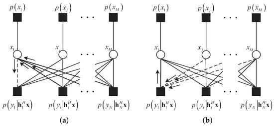
Figure 4.
Linear systems represented by factor graphs: (a) Message from node i = 1 to j = 1. (b) Message from node j = 1 to i = 1.
Based on the factor graph shown in Figure 4, we can get the expression of the sum–product algorithm based on the factor graph:
where is a QPSK signal. By simplifying the sum–product algorithm, we can obtain the core iterative formulation of the AMP algorithm as follows: [33]:
where , , , , . Because the channel is time-varying, we can write the channel as , and , is the estimated noise power. We assume that the power of the noise is Gaussian white noise, so it does not change over time. Function and are defined as:
We assume that the set of MPSK signal mappings is ; then, we can get and :
If M = 4, i.e., the transmit signal is a QPSK signal, we can further simplify the above function as:
3.3. GMM Time-Varying Channel Estimation Based on AR-HMM Model
In the preceding section, we utilized a channel estimation method grounded on superimposed training sequences, essentially employing the least squares (LS) method. It capitalizes on the power gain inherent in the superimposition of cyclic training sequences, making it effective even with lower SNRs. However, this method underutilizes a priori information, rendering it inefficient in practical scenarios. To enhance its efficacy, we refine the channel estimation method by incorporating coarse channel estimation and message-passing-based equalization, introducing a time-varying channel model-based approximate message passing channel estimation approach. Additionally, the superimposed training sequence method proposed earlier proves ineffective during rapid channel variations. In such instances, the asynchronous superimposition of individual cyclic training sequences due to channel influence or overlapping channels results in a composite channel matrix, leading to substantial errors during equalization. To address this issue, we assume a relationship between preceding and subsequent channel changes, conforming to AR-HMM.
where is the AR coefficient. If converted to matrix form expression, we can rewrite it as:
We assume that the channel distribution at each moment obeys a Gaussian mixture distribution, i.e.,
Since underwater acoustic channels are generally considered to be multipath channels with significant sparsity properties, we denote the channel as . This allows us to represent it as a Gaussian mixture distribution as follows:
where denotes the complex Gaussian distribution. We assume that there are K independently and identically distributed elements in .
We can then calculate the Bayesian estimate of using the probability distribution of , i.e., calculate the conditional expectation of :
where:
However, it is very difficult and extremely computationally intensive to try to solve the two equations above, and we need to know the a priori information first. Therefore, we first estimate each time using the AMP algorithm and use the EM algorithm to learn the hyperparameters after each iteration.
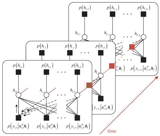
In fact, we can see that Equation (34) is the maximum a posteriori probability estimation, so we still use the AMP-based iterative algorithm, and the main iterative steps are still Equations (19)–(22). Only this time, the estimation object is the channel instead of the sequence to be detected, and we can update the channel estimation method based on AMP with the factor graph in Figure 5.
where , , , , and , is the estimated noise power.
The Toeplitz matrix used in channel estimation is generated from our estimated signal and the transmit signal reconstructed from the loop training sequence, and what is to be estimated is the channel. However, since the distribution of the channel is different from that of the signal, we update the functions and , and, referring to Appendix A, we can obtain the modified functions under GMM as follows:
After the AMP iteration is stopped, the posterior probability density function is obtained as ; then, we can get:
where ,. We substitute the distribution in Equation (32) into Equation (43) to obtain:
where
However, as we can see from the previous steps, we do not know the hyperparameters during the iteration process, so we introduce the EM algorithm for hyperparameter learning during each iteration. The steps of learning can be written:
According to the EM algorithm in reference [34], we can get the iterative equation:
And we can learn the parameters of the GMM at the same time as we learn the parameters of the noise.
where , . The initialization conditions for these parameters are , , , and .
It is worth noting that our iterative algorithm only obtains the channel estimation results for the current block, and based on the assumptions of the AR-HMM model in the previous section, we believe that the channel, although changing at the before and after moments, is strongly correlated within a short period of time, especially in terms of the neighboring before and after channels. To make better use of this correlation, we can get the factor graph as in Figure 5.
From Figure 5, we can see that although the description based on the AR-HMM model does not have a direct impact on the channel estimation of each time period, it still has a very close impact on the before and after channel according to the principle of factor graph message passing. When we get the estimation of , the other factors connect to will no longer have an impact on the node . So by removing the impact of the other nodes, we can get the factor graph of the AR-HMM network as in Figure 6.
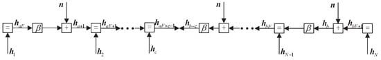
To better describe the estimated channel and the relationship between the implied channel and the final estimated channel, we refer to the references [26,27], wherein the FFG factor graph is used. Obviously, this description of the delay position before and after the channel does not change much, so before we proceed with this step, we must reduce the effect caused by channel Doppler by Doppler compensation.
According to the HMM algorithm, we can get the forward update coefficient by combining the idea of message passing based on the factor graph as:
In the above equation, is the estimated channel vector, and is a transformation with respect to the measurement matrix, which is computed by referring to reference [25]. Due to the AR-HMM assumption, we can obtain the following relationship:
where . Obviously, for the first channel, there is no forward channel transmitting information, so we can get:
Similarly, we can get backward message update coefficients:
And both satisfy the relationship:
Similarly, for one of the rightmost channels, again there are no messages from the backward direction, so for the last piece of the signal, we consider that:
Finally, by fusing the forward and backward messages at moment t, we obtain the forward–backward algorithm based on the AR-HMM model:
In this way, based on the channel obtained from the EM-GMM-AMP channel estimation in the previous section, we can get the channel estimation result for each sub-block, and then this channel estimation result will be used to update the channel coefficients by the HMM-based forward–backward algorithm. Then fed back to the decoding side for iterative decoding and a new round of channel estimation until the iteration is completed.
Of course, we find that there are some other coefficients for which updates do not appear in the iterations of the algorithm, e.g., the mixing coefficients L in the GMM model and the correlation coefficients in the AR-HMM model. Regarding the model of the GMM, in reference [34], Vila proposed a method based on the great likelihood estimation to estimate the order L of the GMM, we use the estimation results based on the superposition of the training sequences for the computation of the L taps. For the channel correlation coefficient, since we have a coarse estimation, the channel correlation coefficient can be derived from the correlation coefficients of the neighboring channels, and this step can also be obtained from the part of superimposed training sequences in the previous section. Then, we statistically average the correlation coefficients obtained as used by forward–backward algorithms based on the temporal correlation of the AR-HMM model.
At this point, the derivation of our algorithm related to superimposed training sequences is complete, and the algorithm will be subsequently validated with out-of-field experiments.
4. Numerical Results
4.1. Simulation
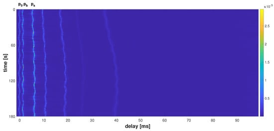
To validate the proposed algorithm in this paper, we executed simulation experiments on a system with the time-varying channel matrix proposed in this paper. In the simulation, we used the time-varying channel model proposed by Stojanovic in [20], which is the channel shown in Figure 7. The delay of this channel changes over time, indicating that we will extract some channels from this series of time-varying channels as simulation channels. The way we add channels is in the form of a time-varying channel matrix as in Equation (8), so we extract the channels and then construct a Toeplitz-like matrix based on the extracted channels, pass the channels in the baseband, and then add Gaussian white noise.
The parameters used in this simulation and subsequent field experiments are listed in Table 1.

Initially, we simulated channel estimation with EM-AMM-AMP. The channel estimation results of the first sub-block are depicted in Figure 8.
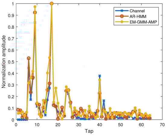
The figure shows the actual channels used, the estimated results of the EM-GMM-AMP algorithm, and the updated CSI with AR-HMM. From the figure, it can be seen that after iteration, the channel estimation based on the EM-GMM-AMP algorithm has achieved a relatively accurate result. Then, after being updated by the AR-HMM forward–backward algorithm, the channel estimation is closer to the actual channel, and in this case, the channel equalization effect is also better. The time-varying communication scheme proposed in this article is complex and not solely based on channel estimation performance. Therefore, we simulated the algorithm proposed in this article and compared it with similar algorithms in reference [26].
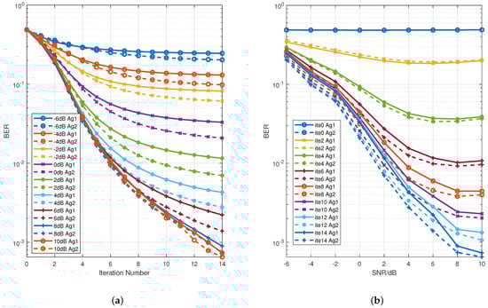
We simulated the signal under different SNRs and iteration times and with a Monte Carlo number of 2000. The main comparison is between the method from reference [26] and the algorithm proposed in this paper. Algorithm 1 in Figure 9 refers to the method based on Gaussian message passing from reference [26]; Algorithm 2 is the algorithm proposed in this paper. We can see from Figure 9a that when the SNR is low, the iterative method based on AMP equalization and GMM-AMP channel estimation proposed in this paper is significantly better than the methods in the reference literature. However, as the SNR increases, the difference between the two gradually narrows. The reason for this phenomenon may be that as the SNR increases, the factors affecting the system, such as the influence of time-varying speed and superimposed pilot power, change. This impacts the correlation coefficients when updating AR-HMM channel information. From Figure 9b, it can be seen that the algorithm proposed in this paper has similar performance to the reference algorithm when the number of iterations is not high. However, as the number of iterations increases, the algorithm proposed in this paper performs better, which is also confirmed in Figure 9a. Therefore, considering all factors, the algorithm proposed in this paper has certain advantages in performance. Nevertheless, a substantial disparity remains between the simulation environment and the real underwater acoustic channel; the actual effect of our system is still based on the field experiment effect, and the simulation is only for reference.
4.2. Field Experiments
Previously, we analyzed the algorithm proposed in this article via a simulation, but the system is a relatively complex communication system, and it is difficult to describe the overall effect through simple simulation experiments. Therefore, we conducted the following two experiments to research this soft iterative system.
4.2.1. Movement Experiment in Pool at Harbin Engineering University
In order to study the communication performance of the soft iterative system using time-varying channels, we conducted mobile UAC experiments in the channel pool at Harbin Engineering University in 2019. The experimental parameters are shown in Table 1. To verify the impact of different time-varying channels on communication performance, we conducted experiments using horizontal and vertical movement. The experimental layout is shown in Figure 10.
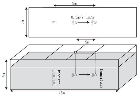
Under the condition of horizontal movement, we set the maximum distance for transmission and reception as 9 m, and the distance for the signal to cycle through is 5 m. The length of one frame of the signal is approximately 5.5 s. So the speed of horizontal movement is estimated to be between 0.6 m/s and 1 m/s. Under vertical movement conditions, due to the shallowness of the pool, we did not move in a single direction, but instead moved up and down, simulating the up–down surge in situations with large waves. We went up and down from a depth of 2 m to 3 m but at a slow speed. For UAC, SNR is a very important parameter. We take the blank signal around the synchronous signal as noise and estimate the SNR in the experiment as:
Based on the experimental data of the pool, we obtained the channel estimation results in the experiment as shown in Figure 11. It can be seen from the figure that the channel changes severely no matter whether it moves horizontally or vertically. The difference is that the horizontally moving channel has an obvious tilt because the transducer moves relatively. The tilt in Figure 11a reflects the influence of Doppler. Because there are no waves and it is very quiet in the pool, the channel in the static state is shown in Figure 11b, and its channel correlation coefficient is shown in Figure 11e, which is almost time invariant. For the channel in the case of vertical movement, it can be seen that its change is also quite intense, but it is interesting that its correlation coefficient has a significant increase at the time of 1.5 s because it moves up and down in the pool, so we infer that at a certain time, the height is the same as the previous time, so this relatively high correlation appears.
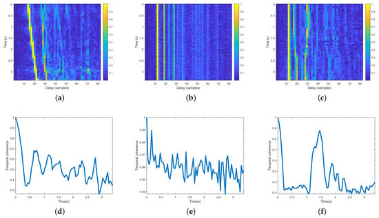
Figure 11.
Channel estimation results of pool experiment: (a) Channel estimated during horizontal movement. (b) Channel estimated when static. (c) Channel estimated during vertical movement. (d) Time correlation coefficient during horizontal movement. (e) Time correlation coefficient when static. (f) Time correlation during vertical movement.
In the static case, BER can be zero after one iteration, so we do not calculate the corresponding error rate. Table 2 shows the decoding results under the condition of horizontal movement. The left side shows the time-varying channel update based on Gaussian message passing, which is the method proposed in reference [26]. The right side shows the time-varying channel update based on GMM and the iterative equalization algorithm based on AMP proposed in this paper. Table 3 shows the results under the condition of vertical movement. The corresponding methods in the table are consistent with Table 2. Moreover, we estimated that the SNR of the pool experiment is about 23 dB.
Table 2.
The error rate of decoding performance under horizontal movement using different algorithms.
We can see from Table 2 and Table 3 that both the GMP and EM-GMM-AMP algorithms work well in the high-SNR situation, and the number of iterations required is less in the case of vertical movement. The performance of the proposed algorithm is better than that of the reference algorithm. In Table 2, we can see that the reference algorithm still has error code after several iterations in the third block, and the method proposed in this paper can achieve zero error code. In addition to the better performance of the algorithm proposed in this paper, the reason may also be the correlation coefficient mismatch. In the Songhua Lake experiment, we focused on a chosen of length of the sub-block in the transmitter and the correlation coefficient in the receiver.
4.2.2. Songhua Lake Mobile Communication Experiment
We conducted a mobile UAC experiment in Songhua Lake, Jilin Province, in June 2019. In this experiment, both the transmitter and receiver were shipborne, and the horizontal distance between the two ships was about 400 m to 1400 m. The receiving ship was anchored, while the transmitting ship drifted with the waves. According to the time and drift distance, it is considered that the transmitting ship floats at an average speed of about 0.6 m/s, and the distance from the receiving ship gradually increases. We also carried out an experiment wherein the transmitting transducer moved up and down. The experimental arrangement is shown in Figure 12.
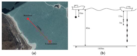
As shown in Figure 12b, during the Songhua Lake experiment, a SIMO UAC experiment was conducted using one transmitter and five receivers. The depth of the transmitter was 10 m, and the reception depths were from 15 m to 35 m. Interestingly, even if the horizontal distance was the same, the power of the received signal varied greatly. The signal at about 30 m was much greater than that at other depths in the 400 m experiment. The combined measured sound velocity gradient data at the receivers for our experiment at Songhua Lake is shown in Figure 13a. We simulated the sound propagation based on a ray model; the result is shown in Figure 13b. We found that in this case, the relationship between the actual received signal and the depth is consistent with the simulation. Under such conditions of a negative gradient of the speed of the sound, there are significant differences in the intensity of the received signals at different depths. So when conducting a short-range UAC experiment in the summer, we should consider not only the communication distance but also the sound propagation conditions.
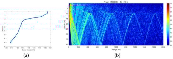
Figure 13.
Simulation of sound propagation in Songhua Lake: (a) sound velocity gradient and (b) sound propagation simulation based on Bellhop.
Because the duration of the Songhua Lake experiment was long and the duration of a frame signal was not very long, the transmission distance ranged from 400 m to 1400 m. The SNRs were between 6 dB and 20 dB. According to the received data of the Songhua Lake experiment, we estimated channels in different situations, and the results are shown in Figure 14. Figure 14a–c correspond to the time-varying channels under the conditions of horizontal movement, static, and vertical movement. It can be seen that, similar to the pool experiment, the Songhua Lake experiment data also have the strongest time-varying signal when moving horizontally. Because these data are the result of synchronization and coarse Doppler compensation, we do not see the result as shown in Figure 11a. Moreover, due to the increase in distance, the impact of slow movement in the vertical direction on the channel change is not as obvious as that in the pool. According to the changes from Figure 11, Figure 12, Figure 13 and Figure 14, we infer that in the actual marine environment, especially in the case of a long distance, the impact of relative movement in the horizontal direction on the communication channel is more severe than that in vertical direction.
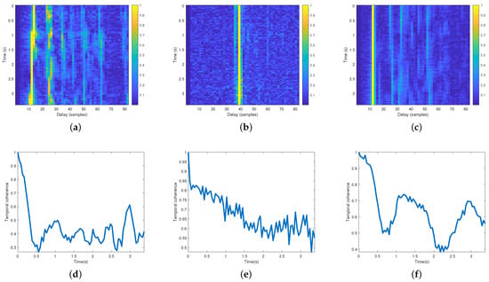
Figure 14.
Channel estimation results of Songhua Lake experiment: (a) Channel estimated during horizontal movement. (b) Channel estimated when static. (c) Channel estimated during vertical movement. (d) Time correlation coefficient during horizontal movement. (e) Time correlation coefficient when static. (f) Time correlation during vertical movement.
It can be predicted that the decoding performance of the first two of the above three channel conditions will be better than that of the third case. Therefore, when conducting the Songhua Lake experiment, we mainly verified the impact of different sub-block lengths and changing correlation coefficients on the decoding performance of the signal under horizontal movement. We compared the proposed algorithm with the reference algorithm in the pool experiment, so the communication system scheme we adopt in this section is the one we proposed.
The experimental results of the Songhua Lake experiment validate the effectiveness of the proposed algorithm for processing time-varying channels based on the correlation coefficient and different block lengths. The correlation coefficient is linked to the pace of channel changes. In general, the smaller the correlation coefficient, the faster the channel changes and the shorter the block length we use. Table 4 shows the data processing results of the Songhua Lake experiment. We compared the decoding performance of different sub-block lengths and the value of the correlation coefficient that performs best. In addition, in order to achieve a certain comparison effect, we compared each group of data in both close and far distance situations. The second row in Table 4 is SNRs obtained from receiving data testing: the SNRs of data at 400 m are generally 6–8 dB, and the SNRs of data at 1400 m are from 11 dB to nearly 17 dB. From the table, we can see that when the correlation coefficient is low, using a short sub-block strategy has better performance. When the correlation coefficient approaches 1, the system basically degenerates into a turbo equalization system [35]. As mentioned in Section 3, the correlation coefficient was estimated from . According to the experimental results from Songhua Lake, we can preliminarily deduce that the SNR plays a crucial role in achieving accurate decoding results in time-varying channels. In our proposed iterative underwater acoustic communication receiver with TC-GMM-AMP algorithm, accurate estimation of the correlation coefficient and selecting an appropriate sub-block length are both essential aspects. With suitable parameters, satisfactory decoding outcomes can be attained even with a low SNR.
Overall, the time-varying channel UAC system proposed in this paper achieved good results in two shallow mobile underwater acoustic channels: a pool experiment and a lake experiment—both with vertical and horizontal movement. However, the system has many parameters, requires many iterative operation modules, and has large overall computation. In our future work, we must overcome these problems.
5. Conclusions
In summary, we can see that for UAC, the changes to the channel structure caused by relative motion are inevitable in the signal processing process. Therefore, we proposed a time-varying channel representation method based on class Toeplitz matrix representation. In order to obtain the time-varying channel matrix, we adopted the method of superimposed training sequences, and further, we proposed the AMP equalization of QPSK signals based on channel estimation as well as the EM-GMM-AMP time-varying channel estimation method based on a soft information iteration of reconstructed signals and on the basis of using power stacking of superimposed training sequences for coarse channel estimation. And we updated the channel information based on the time correlation of the AR-HMM model to estimate channel information iteratively. Then, we used the updated CSI for iterative equalization until the expected number of iterations was reached. Finally, we validated the proposed algorithm based on simulation data, pool experiments, and lake experiments. The simulation data and field experiment results show that the time-varying channel underwater communication method based on superimposed training sequences proposed in this paper has very good application prospects under non-severe time-varying conditions and can achieve good results in field experiments with less severe time-varying conditions.
Author Contributions
Conceptualization, L.L.; methodology, L.L.; software, L.L.; validation, X.H.; formal analysis, L.L.; writing—original draft preparation, L.L.; writing—review and editing, X.H. and W.G.; visualization, X.H.; supervision, W.G.; project administration, X.H.; funding acquisition, X.H. All authors have read and agreed to the published version of the manuscript.
Funding
This research was funded by the National Key R&D Program of China (2021YFC2801200).
Data Availability Statement
Please contact the author for data requests.
Acknowledgments
The authors are grateful to the anonymous reviewers and for the research funding support.
Conflicts of Interest
The authors declare no conflicts of interest.
Appendix A. The Derivation of Denoising Function η(·,·) and κ(·,·) in GMM-AMP Channel Estimation
To simplify the symbols, we simplify the signal to a real number signal in the derivation process and omit any unused subscripts or superscripts.
The AMP algorithm’s inference of signals with different prior information mainly involves changing different and functions for different PDFs. To simplify this process, we denote as .
According to the definitions of and :
We can write as:
is the normalization coefficient and is constant when we compute and . And it is defined as:
Due to our assumption that the distribution of the channel follows the Gaussian mixture distribution from Equation (32), by substituting it into Equation (A4), we can obtain:
Because the order of exchanging integrals and summing remains unchanged, and because the integrals are independent of , they can be extracted as constants. Therefore, we can obtain:
The term in Equation (A6) can be represented by a Gaussian function. We can transform Equation (A6) into:
According to the Gaussian product theorem, we can get:
The function is independent of h, so we can propose integration outside and can write Equation (A9) as:
According to the definition of a Gaussian distribution, the integration within the integration domain is one, so the above equation can ultimately be transformed into:
Next, we can calculate according to the definition of , and according to Equation (A1), we can write as:
Because is constant, we just need to calculate the inner part of the integral first:
According to the definition of a Gaussian distribution, is the mean of h. We substitute into Equation (A14). Then by substituting , we can obtain :
Then, we write as:
Because has been calculated, what we need to calculate is the first part on the right side of the equal sign in Equation (A16). Just like we derived it in Equations (A9) and (A10), we can write this part as:
We define this as , and then we can obtain:
At this point, the denoising function of the AMP algorithm based on the GMM distribution has been derived.
References
- Dao, N.-N.; Tu, N.H.; Thanh, T.T.; Bao, V.N.Q.; Na, W.; Cho, S. Neglected infrastructures for 6G—Underwater communications: How mature are they? J. Netw. Comput. Appl. 2023, 213, 103595. [Google Scholar] [CrossRef]
- Song, A.; Stojanovic, M.; Chitre, M. Editorial underwater acoustic communications: Where we stand and what is next? IEEE J. Ocean. Eng. 2019, 44, 1–6. [Google Scholar]
- Yang, T. Properties of underwater acoustic communication channels in shallow water. J. Acoust. Soc. Am. 2012, 131, 129–145. [Google Scholar] [CrossRef] [PubMed]
- Molisch, A.F. Wideband and Directional Channel Characterization. In Wireless Communications; John Wiley & Sons: New York, NY, USA, 2011; pp. 101–123. [Google Scholar] [CrossRef]
- Zhang, X.; Yang, P.; Wang, Y.; Shen, W.; Yang, J.; Wang, J.; Ye, K.; Zhou, M.; Sun, H. A Novel Multireceiver SAS RD Processor. IEEE Trans. Geosci. Remote. Sens. 2024, 62, 1–11. [Google Scholar] [CrossRef]
- Yang, P. An imaging algorithm for high-resolution imaging sonar system. Multimed. Tools Appl. 2023, 83, 31957–31973. [Google Scholar] [CrossRef]
- Efron, B. Large-Scale Inference: Empirical Bayes Methods for Estimation, Testing, and Prediction; Cambridge University Press: Cambridge, UK, 2012; Volume 1. [Google Scholar]
- Minka, T.P. A Family of Algorithms for Approximate Bayesian Inference. Ph.D Thesis, Massachusetts Institute of Technology, Cambridge, MA, USA, 2001. [Google Scholar]
- Bernardo, J.; Girón, F. A Bayesian analysis of simple mixture problems. Bayesian Stat. 1988, 3, 67–78. [Google Scholar]
- Donoho, D.L.; Maleki, A.; Montanari, A. Message-passing algorithms for compressed sensing. Proc. Natl. Acad. Sci. USA 2009, 106, 18914–18919. [Google Scholar] [CrossRef] [PubMed]
- Zou, Q.; Yang, H. A Concise Tutorial on Approximate Message Passing. arXiv 2022, arXiv:2201.07487. [Google Scholar]
- Rangan, S. Generalized approximate message passing for estimation with random linear mixing. In Proceedings of the 2011 IEEE International Symposium on Information Theory Proceedings, St. Petersburg, Russia, 31 July–5 August 2011; pp. 2168–2172. [Google Scholar]
- Rangan, S.; Schniter, P.; Fletcher, A.K. Vector approximate message passing. IEEE Trans. Inf. Theory 2019, 65, 6664–6684. [Google Scholar] [CrossRef]
- Ma, J.; Ping, L. Orthogonal amp. IEEE Access 2017, 5, 2020–2033. [Google Scholar] [CrossRef]
- Takeuchi, K. Convolutional approximate message-passing. IEEE Signal Process. Lett. 2020, 27, 416–420. [Google Scholar] [CrossRef]
- Liu, L.; Huang, S.; Kurkoski, B.M. Memory approximate message passing. In Proceedings of the 2021 IEEE International Symposium on Information Theory (ISIT), Melbourne, Australia, 12–20 July 2021; pp. 1379–1384. [Google Scholar]
- Luo, M.; Guo, Q.; Jin, M.; Eldar, Y.C.; Huang, D.; Meng, X. Unitary approximate message passing for sparse Bayesian learning. IEEE Trans. Signal Process. 2021, 69, 6023–6039. [Google Scholar] [CrossRef]
- Tian, Y.N.; Han, X.; Yin, J.W.; Liu, Q.Y.; Li, L. Group sparse underwater acoustic channel estimation with impulsive noise: Simulation results based on Arctic ice cracking noise. J. Acoust. Soc. Am. 2019, 146, 2482–2491. [Google Scholar] [CrossRef] [PubMed]
- Bello, P. Characterization of Randomly Time-Variant Linear Channels. IEEE Trans. Commun. Syst. 1963, 11, 360–393. [Google Scholar] [CrossRef]
- Qarabaqi, P.; Stojanovic, M. Statistical characterization and computationally efficient modeling of a class of underwater acoustic communication channels. IEEE Journal of Oceanic Engineering 2013, 38, 701–717. [Google Scholar] [CrossRef]
- Zhang, Y.; Zhu, J.; Wang, H.; Shen, X.; Wang, B.; Dong, Y. Deep reinforcement learning-based adaptive modulation for underwater acoustic communication with outdated channel state information. Remote. Sens. 2022, 14, 3947. [Google Scholar] [CrossRef]
- Wan, L.; Zhou, H.; Xu, X.; Huang, Y.; Zhou, S.; Shi, Z.; Cui, J.H. Adaptive modulation and coding for underwater acoustic OFDM. IEEE J. Ocean. Eng. 2014, 40, 327–336. [Google Scholar] [CrossRef]
- Sun, D.; Wu, J.; Hong, X.; Liu, C.; Cui, H.; Si, B. Iterative double-differential direct-sequence spread spectrum reception in underwater acoustic channel with time-varying Doppler shifts. J. Acoust. Soc. Am. 2023, 153, 1027–1041. [Google Scholar] [CrossRef] [PubMed]
- Liu, Y.; Zhao, Y.; Gerstoft, P.; Zhou, F.; Qiao, G.; Yin, J. Deep transfer learning-based variable Doppler underwater acoustic communications. J. Acoust. Soc. Am. 2023, 154, 232–244. [Google Scholar] [CrossRef] [PubMed]
- Guo, Q.; Ping, L.; Huang, D. A low-complexity iterative channel estimation and detection technique for doubly selective channels. IEEE Trans. Wirel. Commun. 2009, 8, 4340–4349. [Google Scholar]
- Yang, G.; Guo, Q.; Ding, H.; Yan, Q.; Huang, D.D. Joint message-passing-based bidirectional channel estimation and equalization with superimposed training for underwater acoustic communications. IEEE J. Ocean. Eng. 2021, 46, 1463–1476. [Google Scholar] [CrossRef]
- Yang, G.; Guo, Q.; Qin, Z.; Huang, D.; Yan, Q. Belief-Propagation-Based Low-Complexity Channel Estimation and Detection for Underwater Acoustic Communications With Moving Transceivers. IEEE J. Ocean. Eng. 2022, 47, 1246–1263. [Google Scholar] [CrossRef]
- Zhang, Z.; Rao, B.D. Sparse signal recovery with temporally correlated source vectors using sparse Bayesian learning. IEEE J. Sel. Top. Signal Process. 2011, 5, 912–926. [Google Scholar] [CrossRef]
- Zhou, Y.; Tong, F.; Yang, X. Research on co-channel interference cancellation for underwater acoustic mimo communications. Remote. Sens. 2022, 14, 5049. [Google Scholar] [CrossRef]
- Yin, J.; Zhu, G.; Han, X.; Guo, L.; Li, L.; Ge, W. Temporal Correlation and Message-Passing-Based Sparse Bayesian Learning Channel Estimation for Underwater Acoustic Communications. IEEE J. Ocean. Eng. 2024, 1–20. [Google Scholar] [CrossRef]
- Orozco-Lugo, A.G.; Lara, M.M.; McLernon, D.C. Channel estimation using implicit training. IEEE Trans. Signal Process. 2004, 52, 240–254. [Google Scholar] [CrossRef]
- Yuan, W.; Li, S.; Wei, Z.; Yuan, J.; Ng, D.W.K. Data-aided channel estimation for OTFS systems with a superimposed pilot and data transmission scheme. IEEE Wirel. Commun. Lett. 2021, 10, 1954–1958. [Google Scholar] [CrossRef]
- Lyu, S.; Ling, C. Hybrid vector perturbation precoding: The blessing of approximate message passing. IEEE Trans. Signal Process. 2018, 67, 178–193. [Google Scholar] [CrossRef]
- Vila, J.P.; Schniter, P. Expectation-maximization Gaussian-mixture approximate message passing. IEEE Trans. Signal Process. 2013, 61, 4658–4672. [Google Scholar] [CrossRef]
- Panhuber, R. Fast, Efficient, and Viable Compressed Sensing, Low-Rank, and Robust Principle Component Analysis Algorithms for Radar Signal Processing. Remote. Sens. 2023, 15, 2216. [Google Scholar] [CrossRef]
Disclaimer/Publisher’s Note: The statements, opinions and data contained in all publications are solely those of the individual author(s) and contributor(s) and not of MDPI and/or the editor(s). MDPI and/or the editor(s) disclaim responsibility for any injury to people or property resulting from any ideas, methods, instructions or products referred to in the content. |
© 2024 by the authors. Licensee MDPI, Basel, Switzerland. This article is an open access article distributed under the terms and conditions of the Creative Commons Attribution (CC BY) license (https://creativecommons.org/licenses/by/4.0/).