A Network-Group Target State and Network Topology Estimation Method Based on Signals Containing Delay, Doppler and Address

Abstract

Network-group targets are a set of objectives that adhere to a shared communication protocol, perform common tasks, and exhibit relatively coordinated movements. Typically, network-group targets emit radar and communication signals. However, they often employ a silent mode to evade our perception. Despite this, they continue to exchange data through their communication networks. By intercepting the communication signals of these targets, this paper proposes a method for estimating the state and network topology of network-group targets based on random finite set (RFS) theory. This method is based on the modeling of network-group targets using a labeled multi-Bernoulli (LMB) RFS. In state estimation, the usual method involves extracting the localization parameters from the signals in the first step and use these parameters for target tracking in the second step. This study focused on estimating the kinematic states of network-group targets using communication signals containing delay and Doppler information received by multiple mobile sensor platforms. The proposed method considers the coherency between frequency-hopping pulses in the signals, resulting in an improved estimation performance. In addition, considering that network-group targets require network access for information exchange, graph theory concepts were utilized to estimate the network topology of network-group targets by address measurement. The simulation results validated the effectiveness of the proposed method and demonstrated its superior performance.

1. Introduction

With the rapid development and maturation of unmanned aerial vehicle (UAV) technology and wireless communication network technology, new concepts, such as UAV swarms and manned–unmanned teaming (MUM-T), have gradually been applied and validated [1,2,3,4]. A UAV swarm refers to the use of multiple UAVs to form a collective group to accomplish tasks, with coordination between them occurring through a wireless communication network. MUM-T refers to the simultaneous control and command of multiple UAVs using a human-piloted aircraft to perform a mission. MUM-T fully leverages the intelligence and experience of a human-piloted aircraft while also utilizing the maneuverability and payload advantages of UAVs. MUM-T can improve efficiency and survivability while reducing the risks of a human-piloted aircraft. These target formations, which are composed of task-oriented groups through wireless communication networks, can be collectively referred to as network-group targets. The collaboration of network-group targets depends on the communication networks. Therefore, analyzing the radiation of network-group targets is expected to improve the state-estimation performance for these targets.

Standard single-target tracking algorithms assume that the target is a point, limiting it to one measurement per target per time only [5,6,7,8]. Researchers have studied the direct position determination (DPD) of targets using radio signals, including techniques such as time difference of arrival (TDOA), frequency difference of arrival (FDOA), and directions of arrival (DOA) [9,10,11,12,13]. Specifically, regarding the moving radiation sources, the estimation of the location by utilizing TDOA and FDOA information was achieved through fixed receiving stations [10]. Considering the multipath situation, based on the sparsity of locations and velocities, a DPD method for passive radar was proposed to estimate the location and velocity of a moving target in a multipath scenario [11]. A novel approach to efficiently solve the cost function of DPD was proposed [12], which requires fewer particles compared with the classical particle filter (PF) to estimate the kinematic state of the moving source. DPD for mobile narrowband sources based on known waveform signals with a Doppler frequency shift was proposed [13]. The proposed DPD is superior to traditional tracking methods in terms of low signal-to-noise ratio (SNR) and limited quantity of data samples. A system-modeling approach employing cyclic spectrum slices was proposed for directly localizing co-channel signals with distinct cyclic frequencies [14]. A deep learning model for direct trajectory tracking has been developed [15], primarily consisting of two main components: a signal-processing component based on convolutional neural networks (CNNs) and a trajectory generation component based on the Transformer architecture. A multi-task learning model designed for joint direct classification and tracking enables the network to further enhance tracking performance by learning the dynamic patterns of different types of targets.

Multi-target tracking (MTT) algorithms, such as multiple hypothesis tracking (MHT) [16] and the joint probabilistic data association filter (JPDAF) [17,18], were designed to solve the problem of tracking targets that may appear and disappear, with the number and trajectories of the targets changing over time. The random finite set (RFS) approach is a novel methodology in MTT that offers a framework for managing multi-target systems while circumventing intricate data association procedures [19,20,21,22,23]. An RFS is a random variable whose values are finite sets. The number of points in a random finite set is random, and the values of these points are also random and unordered. Observation sets and state sets can naturally be represented using random finite sets. Compared with the aforementioned traditional association algorithms, the RFS approach holds considerable advantages in scenarios with numerous observations and an uncertain number of targets.

Group targets are usually classified as either unresolved or resolvable based on their distribution of position measurements [19]. Unresolved targets, which have a larger number of targets that are difficult to differentiate from each other, are not practical to track individually. Hence, collective movements of the entire group were considered. Extended targets can be regarded as a special type of unresolved targets [24,25,26,27]. These targets have the characteristic that each measurement comes from a single target and each extended target can generate multiple measurements. For instance, a high-resolution radar can detect targets occupying multiple resolution cells, resulting in multiple measurements per time step. Resolvable group targets are defined as a collection of targets with relatively stable formations and similar movement patterns [28,29]. In scenarios that involve target tracking with interactive behaviors, various group structure models have emerged as popular choices. These encompass the virtual leader–follower model [30], Markov random field (MRF) model [31], evolutionary network model [32,33], and social force model [34]. A novel multigroup target tracking algorithm, which leverages evolutionary networks and the labeled box particle probability hypothesis density (LBP-PHD) filter, was introduced by Cheng et al. [35] by adding labels to box particles to obtain the trajectory of individual targets within a group and the overall group trajectory, while also avoiding the instability caused by k-means clustering. The group structure is modeled using graph theory, and the cardinality balanced multitarget multi-Bernoulli (CBMeMBer) filtering algorithm is used to estimate the kinematic state of the group targets [36], which further allows for the estimation of the overall group state based on individual target state estimates within the group. The group structure can be described within the framework of the hypergraph theory, which enhances the performance of data association [37]. The structure identification and tracking problem of circular formation movement was studied [38], and a single trajectory was obtained using the labeled multi-Bernoulli (LMB) filter. To address the problem of tracking large-scale multi-structure group targets, a sequential generalized labeled multi-Bernoulli (GLMB) tracking algorithm was proposed by Zhao et al. [39]. Li et al. derived the single-target state transition function (SSTF) from the direct integral solution of the single-target state stochastic differential equation (SDE) [40], and integrated the proposed SSTF-MB filter into the sensor control strategy.

To minimize the perceived risks, the networked targets employ their stealth capabilities and radar silence to execute their missions. However, due to the necessity of communication to ensure the synchronization of information, such as location, these signals do not remain disconnected for extended periods. Instead, they maintain intermittent synchronization, and their beam width is relatively wide. Consequently, researching the state of network-group targets and their network topology holds significant importance. Additionally, to the best of the authors’ knowledge, there was no previous study that explored the state estimation of network-group targets.

The purpose of this study was to develop a method to achieve passive state and network topology estimation of network-group targets within the framework of a labeled RFS. Unlike traditional group target definitions, network-group targets are defined not by motion coordination between targets, but by communication links. This method considers the use of received broadband frequency-hopping communication signals containing time delay and Doppler information to determine the location and velocity of the transmitter and considers the coherence between frequency-hopping pulses to further improve the tracking performance. Furthermore, the method draws upon certain concepts from graph theory and utilizes address information to estimate the network topology, which is a crucial means for a comprehensive and accurate understanding of network spaces. The approach is applicable to scenarios where the network-group targets are distinguishable and the communication signals have a relatively high SNR, allowing for the accurate acquisition of the targets’ states.

The main contributions of this study are as follows:

• Graph theory is introduced to develop a network-group target-state estimation method that incorporates the network topology.
• In order to improve the estimation performance, a likelihood function was established using frequency-hopping communication signals emitted from the network-group targets, including delay and Doppler information.

The remainder of this paper is organized as follows. Section 2 introduces the network-group target and offers an overview of graph theory and the LMB RFS. Section 3 presents a model for the state, measurement, and communication signals of a network-group target. Section 4 proposes an LMB filter specifically designed for network-group targets. The implementation method of the filter, along with track pruning and state extraction methods, is outlined in Section 5. The simulation results are presented in Section 6. Finally, Section 7 provides concluding remarks and summarizes the contributions of this study.

2. Background

2.1. Notation

In this paper, ${\mathsf{\delta }}_{\mathrm{x},\mathrm{y}}$ represents the Kronecker-$\mathsf{\delta }$ function and ${\mathsf{\delta }}_x\left(y\right)$ represents the Dirac $\mathsf{\delta }$ density at $y=x$. $1_S\left(x\right)$ represents the indicator function of the set S, and if $x\in S$, then $1_S\left(x\right)=1$; otherwise, $1_S\left(x\right)=0$. $\left|S\right|$ represents the number of elements in the finite set S. $〈·\left|·\right.〉$ is the integral over all state variables. For continuous functions, $〈f\left|g\right.〉=\int f\left(x\right)g\left(x\right)dx$, and for discrete sequences, $〈f\left|g\right.〉={\sum }_{i=1}^{\infty }f\left(i\right)g\left(i\right)$. $f^{\mathrm{X}}={\prod }_{x\in \mathrm{X}}f\left(x\right)$ is a multi-objective index. $\mathcal{F}\left(\mathbb{X}\right)$ represents all finite subsets of space $\mathbb{X}$. ${\mathcal{F}}_n\left(\mathbb{X}\right)$ indicates all subsets that include n elements.

The state scalar of a single object is represented by a lowercase letter x. The state vector of a single object is represented by lowercase bold letters: $\mathit{x}$. Multiple object states are represented by uppercase letters: X. The corresponding label versions are represented by the regular forms x, x, and X. The spaces are indicated in bold black letters: $\mathbb{L}$. The exclusive union of sets X and Y: $X\uplus Y$.

In signal processing, scalar values are represented in lowercase italic letters: a. The vectors are represented by lowercase italic scripts: a. The matrix is represented by the capital italic script $\mathit{A}$. ${\mathit{I}}_M$ represents the $M\times M$ identity matrix, and ${\mathit{1}}_{M\times 1}$ represents an M-column vector of ones. Here, diag{$\mathit{a}$} represents a diagonal matrix with vector $\mathit{a}$ on the main diagonal.

2.2. Introduction to Network-Group Targets

Network-group participants are geographically dispersed, but interconnected through wireless communication networks. They collaborate and work together to accomplish their tasks. The normal operation of a wireless communication network requires communication protocols that address the efficient and reliable interaction of messages. According to the TCP/IP five-layer model [41], network protocols of wireless communication networks are typically divided into five layers: application, transport, network, data link, and physical. The application layer provides an interface between the user and the network, the transport layer manages the data transmission between two nodes, and the network layer is responsible for routing and forwarding data frames to achieve data transmission between different networks. The data link layer not only divides the bit stream into data frames and performs error detection and correction but is also responsible for the flow control and access control of the data transmitted at the physical layer to ensure reliable data transmission. Finally, the physical layer primarily handles the digital signal transmission. This study primarily involved transport, data link, and physical layers. The following are some of the properties of the wireless communication network investigated in this study.

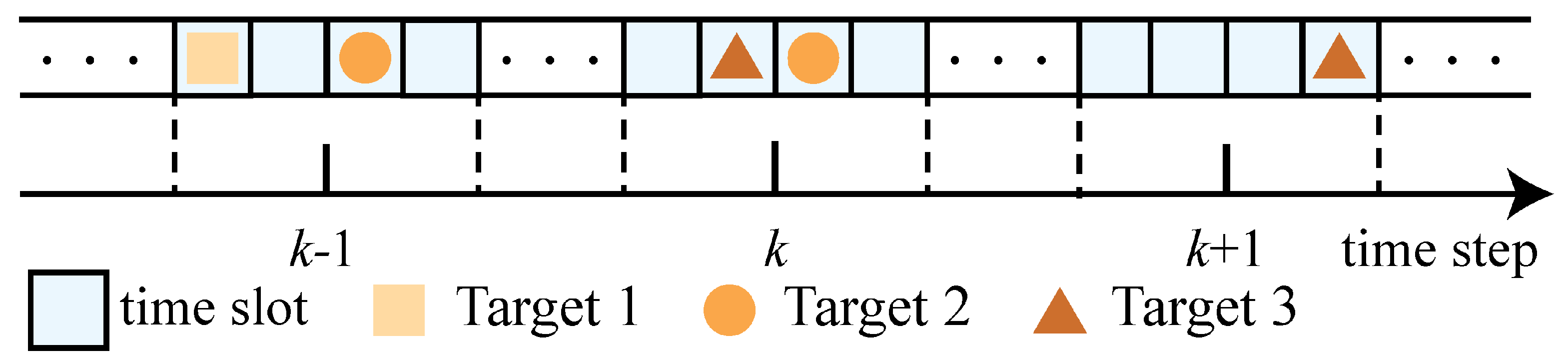
In the transport layer, a time slot serves as the fundamental unit for accessing a wireless communication network. Each participant is assigned several timeslots for signal transmission and reception. Data can be encapsulated in various formats, such as transmitting the same codeword with two pulses or transmitting one codeword with a single pulse.

The data link layer encapsulates the network layer data by adding the source and destination addresses. The address of each target is unique and fixed. The network topology in our study adopted a decentralized structure, and the sublayer protocol used the time-division multiple access (TDMA) method, in which time is divided into nonoverlapping time slots. Each user is assigned a dedicated time slot for data transmission, with each time slot occupied by at most one user. Generally, to minimize interference with other services, the occupancy factor of the time slots is kept low. In addition, this study assumed that network-group targets adopted a lower update rate (sub-second to multi-second levels) for information transmission to reduce the probability of communication signal interference.

In the physical layer, the network-group targets utilize minimum shift keying (MSK) modulation for signal transmission and the carrier frequency hops in a wideband using a specific method.

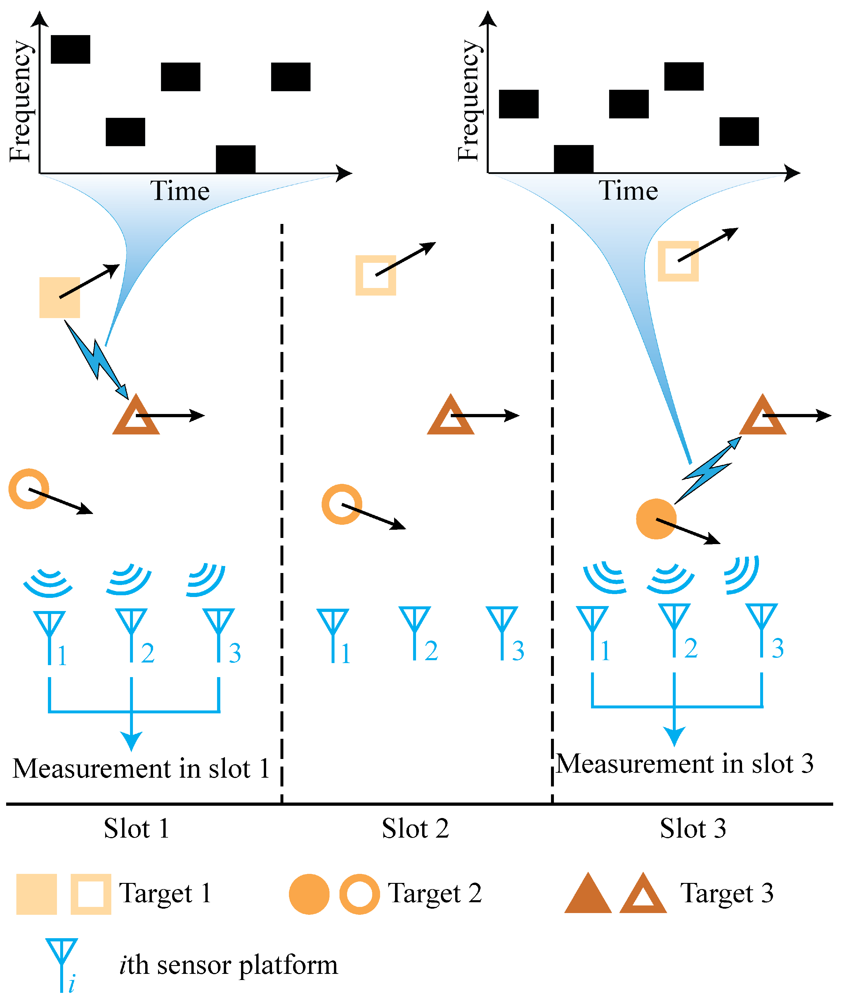
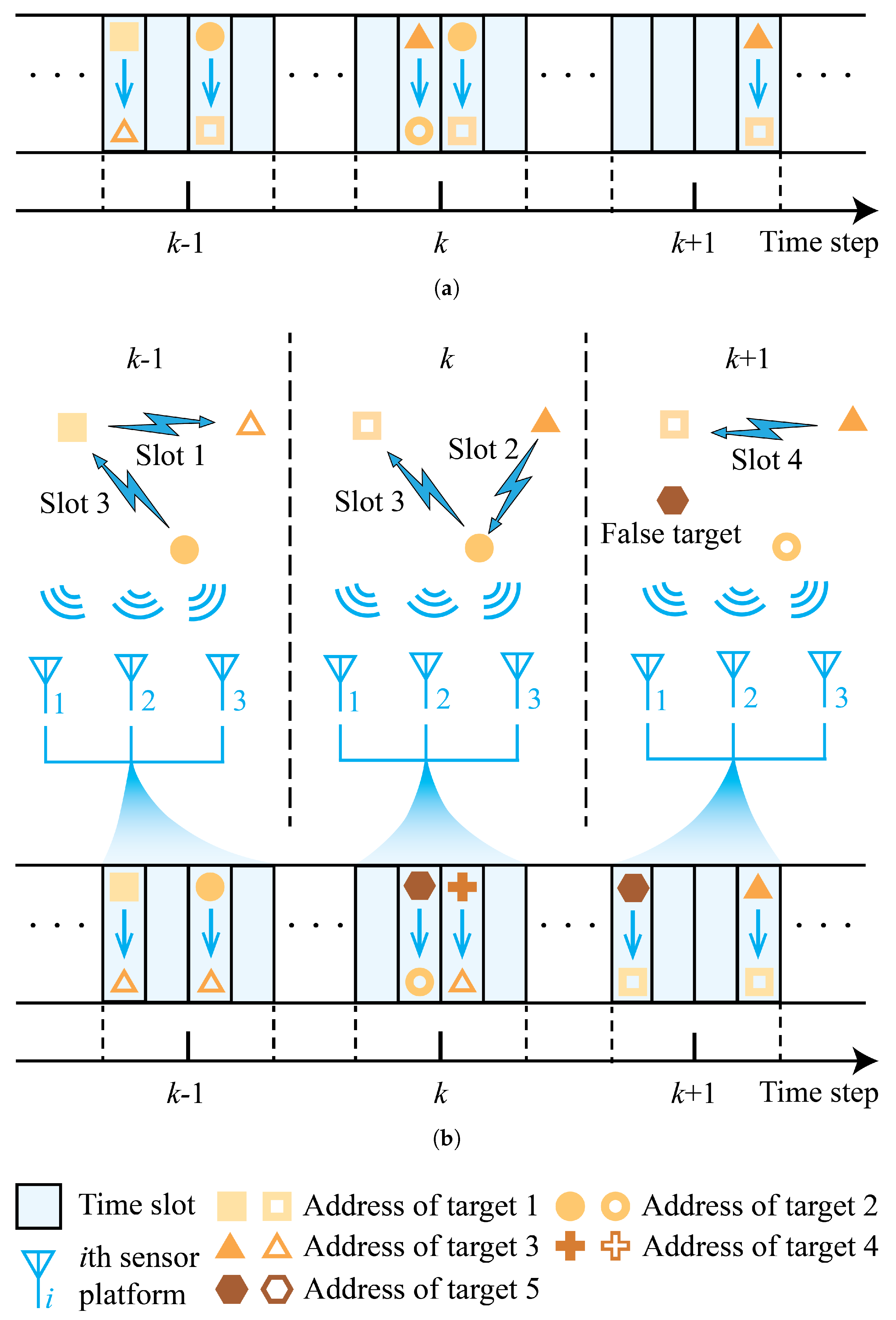
Figure 1 shows a time slot diagram of the three sensor platforms and a network-group with three targets. The main graph in the diagram is a two-dimensional plane that shows the geographical locations of the three sensor platforms and the three network-group targets in three time slots. Each target is represented by a pattern, and the straight black arrow beside the pattern indicates the direction of movement of the target in the slot. The targets move in slightly different directions and not in opposite directions. When a target is transmitted in a time slot, it is represented by a solid pattern; otherwise, it is represented by an empty pattern. The blue lightning symbol with an arrow indicates that the target transmits information during that time slot. Targets 1 and 2 transmit information to target 3 in time slots 1 and 3, respectively, whereas no target is transmitted in time slot 2. Above this diagram is a frequency-hopping pattern diagram for the two transmissions in time slots 1 and 3. In this diagram, each transmission consists of five pulses and the pulse frequency changes over time. Each transmission from the target includes the addresses of the transmitter and receiver. Signals containing time delay, Doppler, and address information were intercepted by the three sensor platforms for further processing.

In this scenario, it is assumed that the antennas used to transmit signals between the network-group targets are omnidirectional rather than narrow-beam types, which is a prerequisite for the sensor platform to intercept communication signals. Our aim was to estimate the kinematic state and network topology of network-group targets by processing signals intercepted from three sensor platforms containing time delay, Doppler, and address information.

2.3. Graph Theory

A graph G consists of a set of vertices $V\left(G\right)=\left\{v_1,\dots ,v_n\right\}$, a set of edges $E\left(G\right)=\left\{e_1,\dots ,e_m\right\}$, and the relationship between them, where two vertices are related by an edge [42].

The directed graph G comprises a set of vertices $V\left(G\right)$, a set of edges $E\left(G\right)$, and a mapping function that associates each edge with an ordered vertex pair. Within this pair, the initial vertex represents the edge tail, and the subsequent vertex serves as the edge head. $u\to v$ denotes the existence of an edge between u and v. The degree d of a vertex refers to the number of times that the vertex appears at the edge.

The adjacency matrix $A\left(G\right)$ of G is a matrix of dimensions $n\times n$, where the element $a_{i,j}$ is the number of edges ending with vertices $v_i$ and $v_j$. In the adjacency matrix $A\left(G\right)$ of directed graph G, the element at $(i,j)$ is the number of edges from $v_i$ to $v_j$. The degree matrix $D\left(G\right)$ of a graph is a diagonal matrix of degrees, that is, $D\left(G\right)=\mathrm{diag}\left\{d_1,\dots ,d_n\right\}$.

The induced subgraph consists of a subset of the vertices of the graph and a set of all edges, with both ends in the subset. A dynamic graph is represented by a set of ordered graphs [43]:

$$D_G=\left\{G_1\dots G_K\right\}$$

(1)

in which K is the number of time steps.

The network topology of network-group targets can be described using directed graphs from graph theory, where vertices represent targets and edges represent information transfer between targets. As illustrated in Figure 1, assuming that the addresses of the three targets are 1, 2, and 3, the targets are represented by vertices denoted by $V\left(G\right)=\left\{1,2,3\right\}$, and the information transfer during the first time slot is represented by edges denoted by $E\left(G\right)=\left\{\left(1\to 3\right)\right\}$.

2.4. LMB RFS

The state space of the target is represented as $\mathbb{X}$, and the label space can be represented as $\mathbb{L}=\left\{{\ell }_i:i\in \mathbb{N}\right\}$, where $\mathbb{N}$ represents the set of positive integers, and ${\ell }_i$ is distinct. The labeled multi-target state is represented by X. The characteristics of the LMB RFS X can be entirely encapsulated within a specific set of parameters $\mathit{q}={\left\{{\epsilon }^{\left(\ell \right)},p^{\left(\ell \right)}\right\}}_{\ell \in \mathbb{L}}$, where ${\epsilon }^{\left(\ell \right)}$ is the probability of the existence of the target ℓ, and $p^{\left(\ell \right)}$ is the probability density of the track when the target ℓ exists. The LMB RFS density with parameter set $\mathit{q}$ can be written as

$$\mathit{q}\left(\mathrm{X}\right)=\Delta \left(\mathrm{X}\right)\omega \left(\mathcal{L}\left(\mathrm{X}\right)\right)p^{\mathrm{X}}$$

(2)

where $\mathcal{L}\left(\mathrm{X}\right)=\left\{\mathcal{L}\left(\mathit{x}\right):\mathit{x}\in \mathrm{X}\right\}$ represents the set of tags in X. $\Delta \left(\mathrm{X}\right)\stackrel{\Delta }{=}{\mathrm{f}\mathrm{f}\mathrm{i}}_{\left|\mathrm{X}\right|}\left(\right|\mathcal{L}\left(\mathrm{X}\right)\left|\right)$ guarantees that the labels of X are distinct. The weight can be written as

$$\omega \left(L\right)=\prod _{{\ell }^{\prime }\in \mathbb{L}}\left(1-{\epsilon }^{\left({\ell }^{\prime }\right)}\right)\prod _{\ell \in L}\frac{1_{\mathbb{L}}\left(\ell \right){\epsilon }^{\left(\ell \right)}}{1-{\epsilon }^{\left(\ell \right)}}$$

(3)

Ignoring the target derivation, the multi-target state in the next time step is the union of the surviving and newborn target states. We assumed that the surviving LMB parameter set is ${\left\{{\epsilon }_{+,s}^{\left(\ell \right)},p_{+,s}^{\left(\ell \right)}\right\}}_{\ell \in \mathbb{L}}$, and the newborn LMB parameter set is ${\left\{{\epsilon }_B^{\left(\ell \right)},p_B^{\left(\ell \right)}\right\}}_{\ell \in \mathbb{B}}$, where $\mathbb{B}$ is the label space of the newborn target. The predicted LMB density is the union of the surviving and newborn LMB densities as follows:

$${\mathit{q}}_{+}={\left\{{\epsilon }_{+,s}^{\left(\ell \right)},p_{+,s}^{\left(\ell \right)}\right\}}_{\ell \in \mathbb{L}}\bigcup {\left\{{\epsilon }_B^{\left(\ell \right)},p_B^{\left(\ell \right)}\right\}}_{\ell \in \mathbb{B}}$$

(4)

and the label space is ${\mathbb{L}}_{+}=\mathbb{L}\bigcup \mathbb{B}$, and $\mathbb{L}\bigcap \mathbb{B}=\varnothing$.

The predicted LMB parameter set is represented by $q_{+}={\left\{{\epsilon }_{+}^{\left(\ell \right)},p_{+}^{\left(\ell \right)}\right\}}_{\ell \in {\mathbb{L}}_{+}}$, and at this time, there are multiple target measurements $Z=\left\{z_1,\dots ,z_{\left|Z\right|}\right\}\in \mathbb{Z}$, where $\mathbb{Z}$ is the measurement space. An LMB parameter set that accurately matches the first moment of the posterior density of multiple targets is

$$\mathit{q}\left(·\left|Z\right.\right)={\left\{{\epsilon }^{\left(\ell \right)},p^{\left(\ell \right)}\right\}}_{\ell \in {\mathbb{L}}_{+}}$$

(5)

For detailed information on the LMB filter, please refer to the paper written by Reuter et al. [44].

3. Problem Statement

3.1. State Modeling of Single Network-Group Target

From the previous section, it can be observed that the basic unit of information transmission for the network group in this study was the time slot. The length of a time slot is usually on the order of ${10}^{-3}$ s, whereas the speed of the aircraft is mostly on the order of ${10}^2$ m/s. Therefore, the distance traveled by the aircraft in one time slot is of the order of 0.1 m. The $N_s$ time slots near each time step can be captured, ensuring that the movement of the network-group target remains within an acceptable range within the $N_s$ time slots. It was assumed that each target can emit at most one communication signal in each capture of the $N_s$ time slots. Figure 2 shows a schematic of the captured time slots of the network-group targets with $N_s=4$, where each square represents a time slot. At three time steps, five communication signals were intercepted, with two signals detected during the first time step, two signals during the second time step, and one signal during the third time step.

An augmented state that consists of two parts was adopted to describe the single network-group target: (1) the kinematic state $x\in \mathbb{X}$ and (2) the address state $u\in \mathcal{C}$, where $\mathcal{C}=\{u_1,\dots ,u_{\left|\mathcal{C}\right|}\}$ is a finite set of addresses. An address probability vector is defined as $c=\{c_1,\dots ,c_{\left|\mathcal{C}\right|}\}$, where $c_i$ represents the probability that the address is the ith address, with ${\sum }_{i=1}^{\left|\mathcal{C}\right|}{c}_i=1$ and $0\le c_i\le 1$. The augmented state vector is defined as $\mathit{x}=(x,c^{\mathrm{t}},c^{\mathrm{r}})$, where $c^{\mathrm{t}}$ is the address probability vector of the network-group target, which can be referred to as the transmitter address probability vector. $c^{\mathrm{r}}$ is the address probability vector of a network-group receiver, which can also be referred to as the receiver address probability vector. The time evolution of kinematic state x of any target can be modeled as follows:

$$x_k=f_k\left(x_{k-1}\right)+w_k$$

(6)

The transition density function is denoted as $f_k$, and $w_k$ represents a Gaussian white noise vector. It was assumed that the probability vector of the address of the transmitter does not change over time, whereas the probability vector of the receiver’s address remains at the initial set value $\{c_1^{\mathrm{r}},\dots ,c_{\left|\mathcal{C}\right|}^{\mathrm{r}}\}$$=\{\raisebox{1ex}{$1$}\!\left/ \!\raisebox{-1ex}{$\left|\mathcal{C}\right|$}\right.,\dots ,\raisebox{1ex}{$1$}\!\left/ \!\raisebox{-1ex}{$\left|\mathcal{C}\right|$}\right.\}$. This is because the true address of the transmitter is fixed, whereas that of the receiver varies each time. The probability density function (PDF) of the Markov state transition is given by

$$\begin{array}{cc}\hfill {\varphi }_{k|k-1}\left({\mathit{x}}_{+}\right|\mathit{x})& ={\varphi }_{k|k-1}(x_{+},c_{+}^{\mathrm{t}},c_{+}^{\mathrm{r}}|x,c^{\mathrm{t}},c^{\mathrm{r}})\hfill \\ \hfill & ={\mathsf{\delta }}_{c_{+}^{\mathrm{t}},c^{\mathrm{t}}}{\mathsf{\delta }}_{c_{+}^{\mathrm{r}},c^{\mathrm{r},1}}{\varphi }_{k|k-1}\left(x_{+}\right|x)\hfill \end{array}$$

(7)

where ${\varphi }_{k|k-1}\left(x_{+}\right|x)$ is the PDF of the Markov transition for the state and $c^{\mathrm{r},1}$ is the initial value of the probability vector for the receiver’s address.

3.2. Measurement Modeling of Single Network-Group Target

If a target is detected, the augmented measurement value is defined as follows:

$${\mathit{z}}_k=\left[z_k^{\mathrm{p}},z_k^{\mathrm{t}},z_k^{\mathrm{r}}\right]$$

(8)

in which $z_k^{\mathrm{p}}$ is a kinematic-related measurement, $z_k^{\mathrm{t}}$ is the address measurement of the transmitter, and $z_k^{\mathrm{r}}$ is the address measurement of the receiver. Both $z_k^{\mathrm{t}}$ and $z_k^{\mathrm{r}}$ are one-hot vectors. For example, $z_k^{\mathrm{t}}=$$[0,1,0]$ represents a total of $\mathcal{C}=3$ address measurements, and the address measurement of the transmitter is the second one, i.e., $u_2$. The address measurement of the receiver is similar. The kinematic measurement model of the target is $z_k^{\mathrm{p}}=$${\mathsf{\tau }}_k(x_k,V_k)$, where V is a random noise vector and ${\mathsf{\tau }}_k$ is the measurement function. The address measurement models of the transmitter and receiver are $z_k^{\mathrm{t}}=\Xi \left(\mathit{r}\right)$ and $z_k^{\mathit{r}}=\Xi \left(\mathit{r}\right)$, respectively, where $\Xi$ is the recognizer of addresses and $\mathit{r}$ represents the signal emitted by the target and received by the sensor platforms. Since the focus of this study was not on signal recognition, it was assumed that the performance of the recognizer can be represented by a confusion matrix defined as

$$\Pi \stackrel{\Delta }{=}{\left[{\pi }_{i,j}\right]}_{\left|\mathcal{C}\right|\times \left|\mathcal{C}\right|}$$

(9)

where ${\pi }_{i,j}=Pr\left(\mathrm{declare}j\right|i\mathrm{is}\mathrm{true})$, and i and j represent addresses. For example, the element ${\pi }_{1,2}^{\mathrm{t}}=Pr(z^{\mathrm{t}}=[0,1,0]|u^{\mathrm{t}}=u_1)$ in the confusion matrix of the address recognizer for the transmitter represents the probability that the transmitter address measurement is recognized as $u_2$ when the actual address of the transmitter is $u_1$.

In this scenario, in addition to the measurements that originate from the target, the measurements received by the sensor platforms included measurements from false targets. The likelihood function for a single network-group target is denoted as

$$g_k\left(\mathit{z}\left|\mathit{x}\right.\right)=g_k\left(z_k^{\mathrm{p}},z_k^{\mathrm{t}},z_k^{\mathrm{r}}\left|x,c^{\mathrm{t}},c^{\mathrm{r}}\right.\right)$$

(10)

Because the determination of the address is purely based on the address probability vector and is independent of the kinematics, (10) can be expressed as

$$g_k\left(\mathit{z}\left|\mathit{x}\right.\right)=g_k\left(z_k^{\mathrm{p}}\left|x\right.\right)g_k\left(z_k^{\mathrm{t}}\left|c^{\mathrm{t}}\right.\right)g_k\left(z_k^{\mathrm{r}}\left|c^{\mathrm{r}}\right.\right)$$

(11)

Figure 3 shows the sequence diagrams of the transmitter and receiver. Figure 3a,b show the actual and recognized sequence diagrams, respectively. The addresses of the transmitter and receiver are determined by identifying the signals intercepted by the sensor platforms.

Only three actual addresses are shown in Figure 3a, whereas five addresses after recognition are shown in Figure 3b. By comparing Figure 3a,b, it can be observed that the recognizer accurately recognized the transmitter and receiver addresses in the first time slot of time step $k-1$ and the fourth time slot of time step $k+1$. However, in the third time slot of time step $k-1$ and second time slot of time step k, the recognizer incorrectly recognized the receiver and transmitter addresses, respectively. In addition, in the third time slot of time step k, the recognizer incorrectly recognized both addresses. In the first time slot of time step $k+1$, which was intended to have no target transmission, a signal transmission occurred because of a false target.

3.3. Signal Modeling of Single Network-Group Target

If a target emits a signal within a time slot, each time slot contains N frequency-hopping pulses, where $T_w$ and $T_p$ are the pulse width and pulse period of the frequency-hopping pulses, respectively. This study assumed that the pulse width and pulse period of the frequency-hopping pulses are fixed.

Assume that at the kth time step in the $n_s$th time slot, the target emits a signal without considering the random delay, and emits a signal at $t=0$ with position ${\mathit{p}}_k$ and velocity ${\dot{\mathit{p}}}_k$. There are a total of L moving sensor platforms, with positions and velocities denoted as ${\mathit{p}}_{k,l}$ and ${\dot{\mathit{p}}}_{k,l}$ ($l=1,\dots ,L$), respectively. In the following derivations, k is omitted. The nth pulse signal from the target can be modeled as

$${\tilde{s}}_n\left(t\right)=s_n\left(t\right)e^{j\phi }{e}^{\mathrm{j}2\pi f_{n}t}$$

(12)

where $\phi$ represents the initial phase of the signal, $f_n$ represents the carrier frequency of the pulse, and $s_n$ represents the complex envelope of the signal. $s_n$ can be written as

$$s_n\left(t\right)=\left\{\begin{array}{cc}{s}_{0,n}\left(t\right)\hfill & \left(n-1\right)T_p\le t<\left(n-1\right)T_w\hfill \\ 0\hfill & \left(n-1\right)T_w\le t<n{T}_p\hfill \end{array}\right.$$

(13)

where $n\in \left\{1,2,\dots ,N\right\}$ represents the nth pulse and $s_{0,n}\left(t\right)$ is unknown. Therefore, the lth sensor platform intercepts the nth pulse signal of the target as follows:

$$r_{l,n}\left(t\right)={\tilde{s}}_n\left(t-{\tau }_l\left(t\right)\right)+w_{l,n}\left(t\right)$$

(14)

where $w_{l,n}\left(t\right)$ is Gaussian white noise with variance ${\sigma }_{l,n}$ and ${\tau }_l\left(t\right)$ is a time-varying delay. Considering the first sensor platform as the reference sensor platform, letting $t^{\prime }=t-{\tau }_1\left(t\right)$, substituting (12) into (14), and setting $t=t^{\prime }$ results in

$$r_{l,n}\left(t\right)=s_n\left(t-\Delta {\tau }_l\left(t\right)\right)e^{\mathrm{j}{\phi }_l}{e}^{\mathrm{j}2\pi f_n\left(t-\Delta {\tau }_l\left(t\right)\right)}+w_{l,n}\left(t\right)$$

(15)

where $\Delta {\tau }_l\left(t\right)={\tau }_l\left(t\right)-{\tau }_1\left(t\right)$ represents the time-varying TDOA between the lth and the first sensor platforms, and ${\phi }_l$ is the unknown phase deviation. Expanding ${\tau }_l\left(t\right)$ in a Taylor series at $t=0$ yields

$$\begin{array}{cc}\hfill {\tau }_l\left(t\right)& ={\tau }_l\left(0\right)+{{\tau }_l}^{\prime }\left(0\right)t+\frac{{{\tau }_l}^{″}\left(0\right)}{2}{t}^2+\dots \hfill \\ \hfill & =\frac{d_l}{c}+\frac{{\dot{d}}_l}{c}t+\frac{{\ddot{d}}_l}{2c}{t}^2+\dots \hfill \end{array}$$

(16)

where $d_l$, ${\dot{d}}_l$, and ${\ddot{d}}_l$ represent the relative distance, velocity, and acceleration between the network-group target and the lth sensor platform, respectively.

Because of the assumption that the signal of each target appears at most once in the kth interception, that is, at time k, the localization of the same source is limited to one time slot. The localization process is short, and the position and velocity are sufficient to reflect the motion dynamics of the target within a short period of time. The information provided by the target’s acceleration over a short period to monitor the situation is not significant. Therefore, we omitted the acceleration information of the target in the above equation, which can be written as

$${\tau }_l\left(t\right)\approx \frac{d_l}{c}+\frac{{\dot{d}}_l}{c}t={\tau }_l\left(0\right)+\frac{{\dot{d}}_l}{c}t$$

(17)

where ${\tau }_l\left(0\right)$ is the time delay from the network-group target to the lth sensor platform at $t=0$. Therefore, the time-varying TDOA can be expressed as

$$\Delta {\tau }_l\left(t\right)={\tau }_l\left(t\right)-{\tau }_1\left(t\right)=\Delta {\tau }_l\left(0\right)+\frac{\Delta {\dot{d}}_l}{c}t$$

(18)

where $\Delta {\tau }_l\left(0\right)={\tau }_l\left(0\right)-{\tau }_1\left(0\right)$$=\frac{∥{\mathit{p}}_l-\mathit{p}∥}{c}$$-\frac{∥{\mathit{p}}_1-\mathit{p}∥}{c}$ represents the TDOA between the signal propagating from the target to the lth receiving sensor platform and the signal propagating to the first sensor platform at $t=0$, whereas $\Delta {\dot{d}}_l={\dot{d}}_l-{\dot{d}}_1$$=\frac{{\left(\dot{\mathit{p}}-{\dot{\mathit{p}}}_l\right)}^{\mathrm{T}}\left({\mathit{p}}_l-\mathit{p}\right)}{∥{\mathit{p}}_l-\mathit{p}∥}-$$\frac{{\left(\dot{\mathit{p}}-{\dot{\mathit{p}}}_1\right)}^{\mathrm{T}}\left({\mathit{p}}_1-\mathit{p}\right)}{∥{\mathit{p}}_1-\mathit{p}∥}$ represents the radial velocity difference between the two sensor platforms relative to the network-group target.

Because the assumption of a fixed pulse period was made in Section 3.3, we can set $t^{\prime }+\left(n-1\right)T_p=t,t^{\prime }\in \left[0,T_p\right]$ and down-convert the received signal to the lth sensor platform using the known carrier frequency $f_n$. Then, let $t=t^{\prime }$ to obtain

$$\begin{array}{c}{r}_{l,n}(t)=s_n(t+(n-1)T_p-\Delta {\tau }_l(0)-\frac{\Delta {\dot{d}}_l}{c}(t+(n-1)T_p))\hfill \\ e^{j{\phi }_l}{e}^{-\mathrm{j}2\pi f_n(\Delta {\tau }_l(0)+\frac{\Delta {\dot{d}}_l}{c}(t+(n-1)T_p))}+w_{l,n}\left(t\right)\hfill \end{array}$$

(19)

Because of the existence of the TDOA change term $\frac{\Delta {\dot{d}}_l}{c}\left(t+(n-1)T_p\right)$ in the signal envelope and the phase term, the term causes changes in both. Assuming a distance difference of the order of ${10}^3$ m, a signal accumulation time of the order of ${10}^{-3}$ s, and a velocity of the order of ${10}^2$ m/s, it can be noted that the influence of the TDOA change term on the slowly varying envelope can be neglected. Hence, the equation can be simplified to

$$\begin{array}{c}{r}_{l,n}(t)=s_n(t+(n-1)T_p-\Delta {\tau }_l\left(0\right))e^{j{\phi }_l}\\ e^{-\mathrm{j}2\pi f_n(\Delta {\tau }_l(0)+\frac{\Delta {\dot{d}}_l}{c}(t+(n-1)T_p))}+w_{l,n}\left(t\right)\end{array}$$

(20)

Let

$${\mathit{s}}_n\stackrel{\Delta }{=}{\left[s_n\left[1\right],\dots ,s_n\left[M\right]\right]}^{\mathrm{T}},\mathit{s}\stackrel{\Delta }{=}{\left[{\mathit{s}}_1^{\mathrm{T}},\dots ,{\mathit{s}}_N^{\mathrm{T}}\right]}^{\mathrm{T}}$$

$${\mathit{w}}_l\stackrel{\Delta }{=}{\left[w_l\left[1\right],\dots ,w_l\left[M\right]\right]}^{\mathrm{T}},\mathit{w}\stackrel{\Delta }{=}{\left[{\mathit{w}}_1^{\mathrm{T}},\dots ,{\mathit{w}}_N^{\mathrm{T}}\right]}^{\mathrm{T}}$$

$$\stackrel{⌢}{\mathit{m}}\stackrel{\Delta }{=}{\left[0,\dots ,M-1\right]}^{\mathrm{T}}$$

$$\tilde{\mathit{m}}\stackrel{\Delta }{=}{\left[-\frac{NM}{2},-\frac{NM}{2}+1,\dots ,\frac{NM}{2}-1\right]}^{\mathrm{T}}$$

$$\mathit{F}\stackrel{\Delta }{=}\frac{1}{\sqrt{NM}}exp\left(-\mathrm{j}2\pi \tilde{\mathit{m}}{\tilde{\mathit{m}}}^{\mathrm{T}}\right)$$

$${\Gamma }_l\stackrel{\Delta }{=}\mathrm{diag}\left\{exp\left(-\mathrm{j}\frac{2\pi }{NM}\Delta {\tau }_l\left(0\right)\tilde{\mathit{m}}/f_s\right)\right\}$$

$${\mathit{A}}_{l,n}\stackrel{\Delta }{=}\mathrm{diag}\left\{exp\left(-\mathrm{j}2\pi f_n(\begin{array}{c}\Delta {\tau }_l\left(0\right){\mathbf{1}}_{M\times 1}+\hfill \\ \frac{\Delta {\dot{d}}_l}{c}(\frac{\stackrel{⌢}{\mathit{m}}}{f_s}+(n-1)T_p{\mathit{1}}_{M\times 1})\hfill \end{array})\right.\right\}$$

$${\mathit{A}}_l\stackrel{\Delta }{=}\mathrm{diag}\left\{{\mathit{A}}_{l,1},\dots ,{\mathit{A}}_{l,n}\right\},{\mathit{E}}_l\stackrel{\Delta }{=}exp\left(j{\phi }_l\right){\mathit{I}}_{NM}$$

where $f_s$ is the sampling frequency. The signal of the network-group target intercepted by the lth sensor platform is

$${\mathit{r}}_l={\mathit{E}}_l{\mathit{A}}_l{\mathit{F}}^{\mathrm{H}}{\Gamma }_l\mathit{Fs}+{\mathit{w}}_l={\mathit{Q}}_l\mathit{s}+{\mathit{w}}_l$$

(21)

where ${\mathit{w}}_l$ follows a Gaussian distribution with a mean of zero and covariance of ${\Lambda }_l={\sigma }_l^2{\mathit{I}}_{NM}$; ${\sigma }_l^2$ represents the variance.

Define

$$\mathit{r}\stackrel{\Delta }{=}{\left[{\mathit{r}}_1^{\mathrm{T}},\dots ,{\mathit{r}}_L^{\mathrm{T}}\right]}^{\mathrm{T}}$$

(22)

$$\mathit{Q}\stackrel{\Delta }{=}{\left[{\mathit{Q}}_1^{\mathrm{T}},\dots ,{\mathit{Q}}_L^{\mathrm{T}}\right]}^{\mathrm{T}},\mathsf{\Lambda }\stackrel{\Delta }{=}diag\left\{{\mathsf{\Lambda }}_1,\dots ,{\mathsf{\Lambda }}_L\right\}$$

so that $\mathit{r}=\mathit{Qs}+\mathit{w}$.

In (8), the kinematic measurement at the kth time step is given by $z_k^{\mathrm{p}}={\mathit{r}}^k$.

4. The Proposed Method

Assuming that the distribution of the augmented spatial PDF in the presence of a target is represented by $s\left(\mathit{x}\right)=s\left(x,c^{\mathrm{t}},c^{\mathrm{r}}\right)$, the density of the augmented LMB parameter set is represented by

$$\begin{array}{cc}\hfill \mathit{q}& ={\left\{{\epsilon }^{\left(\ell \right)},s{\left(\mathit{x}\right)}^{\left(\ell \right)}\right\}}_{\ell \in \mathbb{L}}\hfill \\ \hfill & ={\left\{{\epsilon }^{\left(\ell \right)},p^{\left(\ell \right)}\left(x\right),{\gamma }^{\left(\ell \right)}\left(c^{\mathrm{t}}\right),{\gamma }^{\left(\ell \right)}\left(c^{\mathrm{r}}\right)\right\}}_{\ell \in \mathbb{L}}\hfill \end{array}$$

(23)

where $p\left(x\right)$ is the PDF with the label ℓ for the target kinematic state, and $\gamma \left(c^{\mathrm{t}}\right)$ and $\gamma \left(c^{\mathrm{r}}\right)$ are the PDFs with the label ℓ for the transmitter and receiver addresses, respectively. $p\left(x\right)$, $\gamma \left(c^{\mathrm{t}}\right)$, and $\gamma \left(c^{\mathrm{r}}\right)$ are independent.

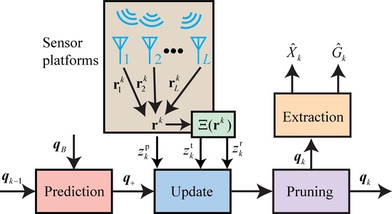
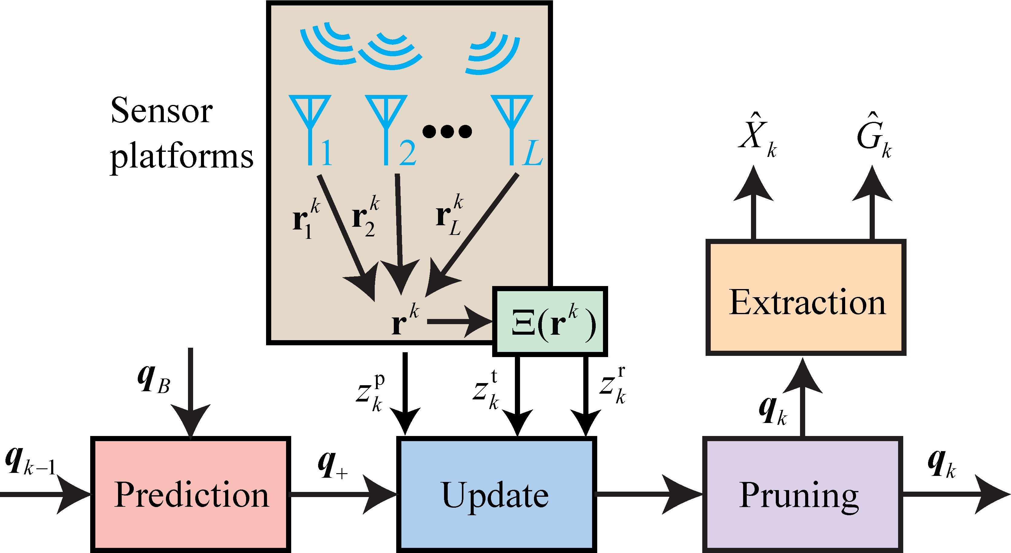
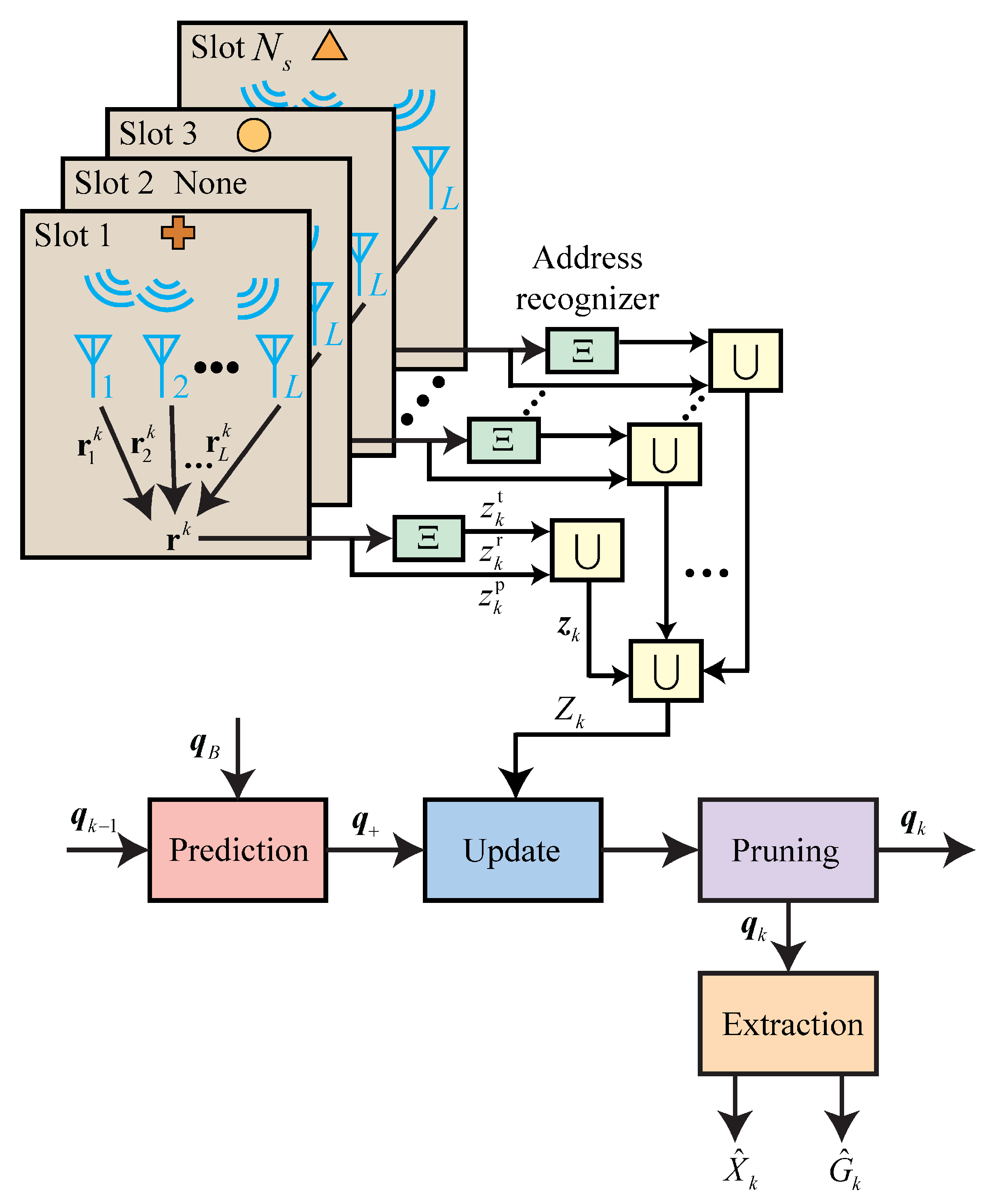
The flowchart of the proposed method is shown in Figure 4. In the prediction step, the predicted LMB parameter set, denoted as ${\mathit{q}}_{+}$, is calculated using the prior LMB parameter set, denoted as ${\mathit{q}}_{k-1}$, and the birth LMB parameter set, denoted as ${\mathit{q}}_B$. The state transition density function, given by (7), is used for this calculation. There are L sensor platforms that listen to signals in time slots of time step k. The signals captured in the occupied time slots are sent to a platform to form a column vector, denoted as ${\mathit{r}}^k$, as shown in (22); each signal in the occupied time slots is transmitted to an address recognizer (represented by the confusion matrix in (9) in this paper) to obtain address measurements $z_k^{\mathrm{t}}$ and $z_k^{\mathrm{r}}$ for the transmitter and receiver, respectively. The augmented measurement for the occupied time slots is denoted as ${\mathrm{z}}_k$, as shown in (7), and the measurement at time step k is denoted as $Z_k$. In the update step, the likelihood function is calculated based on the measurements $Z_k$. After the update step, track pruning is performed based on the existence probability and addresses. Finally, in the extraction step, the trajectory and network topology structure are extracted.

4.1. Prediction

It was assumed that the prior and newborn target distributions are both LMB.

Proposition 1.

Given a set of augmented prior LMB parameters and a set of augmented LMB parameters for births, denoted by

$$\begin{array}{cc}\hfill {\mathit{q}}_{k-1}& ={\left\{{\epsilon }_{k-1}^{\left(\ell \right)},s{\left(\mathit{x}\right)}_{k-1}^{\left(\ell \right)}\right\}}_{\ell \in \mathbb{L}}\hfill \\ \hfill & ={\left\{{\epsilon }_{k-1}^{\left(\ell \right)},p_{k-1}^{\left(\ell \right)}\left(x\right),{\gamma }_{k-1}^{\left(\ell \right)}\left(c^{\mathrm{t}}\right),{\gamma }_{k-1}^{\left(\ell \right)}\left(c^{\mathrm{r}}\right)\right\}}_{\ell \in \mathbb{L}}\hfill \end{array}$$

(24)

$$\begin{array}{cc}\hfill {\mathit{q}}_B& ={\left\{{\epsilon }_B^{\left(\ell \right)},s{\left(\mathit{x}\right)}_B^{\left(\ell \right)}\right\}}_{\ell \in \mathbb{B}}\hfill \\ \hfill & ={\left\{{\epsilon }_B^{\left(\ell \right)},p_B^{\left(\ell \right)}\left(x\right),{\gamma }_B^{\left(\ell \right)}\left(c^{\mathrm{t}}\right),{\gamma }_B^{\left(\ell \right)}\left(c^{\mathrm{r}}\right)\right\}}_{\ell \in \mathbb{B}}\hfill \end{array}$$

(25)

the predicted set of augmented LMB parameters is

$$\begin{array}{cc}\hfill {\mathit{q}}_{+}& ={\left\{{\epsilon }_{+,s}^{\left(\ell \right)},s_{+,s}^{\left(\ell \right)}\left(\mathit{x}\right)\right\}}_{\ell \in {\mathbb{L}}_{k-1}}\bigcup {\left\{{\epsilon }_B^{\left(\ell \right)},s_B^{\left(\ell \right)}\left(\mathit{x}\right)\right\}}_{\ell \in \mathbb{B}}\hfill \\ \hfill & ={\left\{{\epsilon }_{+}^{\left(\ell \right)},s_{+}^{\left(\ell \right)}\left(\mathit{x}\right)\right\}}_{\ell \in {\mathbb{L}}_{+}}\hfill \\ \hfill & ={\left\{{\epsilon }_{+}^{\left(\ell \right)},p_{+}^{\left(\ell \right)}\left(x\right),{\gamma }_{+}^{\left(\ell \right)}\left(c^{\mathrm{t}}\right),{\gamma }_{+}^{\left(\ell \right)}\left(c^{\mathrm{r}}\right)\right\}}_{\ell \in {\mathbb{L}}_{+}}\hfill \end{array}$$

(26)

with label space ${\mathbb{L}}_{+}={\mathbb{L}}_{k-1}\bigcup \mathbb{B}$ (${\mathbb{L}}_{k-1}\bigcap \mathbb{B}=\varnothing$).

For the existence part of the augmented LMB:

$${\epsilon }_{+,s}^{\left(\ell \right)}={\eta }_s^{\left(\ell \right)}{\epsilon }_{k-1}^{\left(\ell \right)}$$

(27)

$$p_{+,s}^{\left(\ell \right)}\left(x\right)=\frac{\int P_S^{\left(\ell \right)}\left(x\right){\varphi }_{k|k-1}\left(x_{+}\right|x)p^{\left(\ell \right)}\left(x\right)dx}{\int P_S^{\left(\ell \right)}\left(x\right)p^{\left(\ell \right)}\left(x\right)dx}$$

(28)

$${\gamma }_{+,s}^{\left(\ell \right)}\left(c^{\mathrm{t}}\right)=\frac{{\gamma }^{\left(\ell \right)}\left(c^{\mathrm{t}}\right)}{\int {\gamma }^{\left(\ell \right)}\left(c^{\mathrm{t}}\right)d{c}^{\mathrm{t}}}$$

(29)

$${\gamma }_{+,s}^{\left(\ell \right)}\left(c^{\mathrm{r}}\right)=\frac{{\gamma }^{\left(\ell \right)}\left(c^{\mathrm{r},1}\right)}{\int {\gamma }^{\left(\ell \right)}\left(c^{\mathrm{r}}\right)d{c}^{\mathrm{r}}}$$

(30)

where $P_S^{\left(\ell \right)}\left(x\right)$ represents the survival probability and ${\eta }_s^{\left(\mathit{\ell }\right)}$ is the survival probability of the target ℓ, which can be expressed as

$$\begin{array}{cc}\hfill {\eta }_s^{\left(\ell \right)}& =〈P_S^{\left(\ell \right)}\left(x\right),s^{\left(\ell \right)}\left(\mathit{x}\right)〉\hfill \\ \hfill & =\int {\gamma }^{\left(\ell \right)}\left(c^{\mathrm{t}}\right)d{c}^t\int {\gamma }^{\left(\ell \right)}\left(c^{\mathrm{r}}\right)d{c}^{\mathrm{r}}\int P_S^{\left(\ell \right)}\left(x\right)p^{\left(\ell \right)}\left(x\right)dx\hfill \end{array}$$

(31)

Therefore,

$$p_{+}^{\left(\ell \right)}\left(x\right)=1_{\mathbb{L}}\left(\ell \right)p_{+,s}^{\left(\ell \right)}\left(x\right)+1_{\mathbb{B}}\left(\ell \right)p_{+,B}^{\left(\ell \right)}\left(x\right)$$

(32)

$${\gamma }_{+}^{\left(\ell \right)}\left(c^{\mathrm{t}}\right)=1_{\mathbb{L}}\left(\ell \right){\gamma }_{+,s}^{\left(\ell \right)}\left(c^{\mathrm{t}}\right)+1_{\mathbb{B}}\left(\ell \right){\gamma }_B^{\left(\ell \right)}\left(c^{\mathrm{t}}\right)$$

(33)

$${\gamma }_{+}^{\left(\ell \right)}\left(c^{\mathrm{r}}\right)=1_{\mathbb{L}}\left(\ell \right){\gamma }_{+,s}^{\left(\ell \right)}\left(c^{\mathrm{r}}\right)+1_{\mathbb{B}}\left(\ell \right){\gamma }_B^{\left(\ell \right)}\left(c^{\mathrm{r}}\right)$$

(34)

Proof. 

The survival probability of target ℓ is represented by

$$\begin{array}{cc}\hfill & {\eta }_s^{\left(\ell \right)}=〈P_S^{\left(\ell \right)}\left(x\right),s^{\left(\ell \right)}\left(\mathit{x}\right)〉=\int {\gamma }^{\left(\ell \right)}\left(c^{\mathrm{t}}\right)d{c}^{\mathrm{t}}\hfill \\ \hfill & \int {\gamma }^{\left(\ell \right)}\left(c^{\mathrm{r}}\right)d{c}^{\mathrm{r}}\int P_S^{\left(\ell \right)}\left(x\right)p^{\left(\ell \right)}\left(x\right)dx\hfill \end{array}$$

(35)

Based on the Markov state transition density in (7), the predicted LMB has a partially augmented track probability density, which can be expressed as

$$\begin{array}{cc}\hfill s_{+,s}^{\left(\ell \right)}\left(\mathit{x}\right)& =\frac{〈P_S^{\left(\ell \right)}\left(x\right){\varphi }_{k\left|k-1\right.}\left({\mathit{x}}_{+}\left|\mathit{x}\right.\right),s^{\left(\ell \right)}\left(\mathit{x}\right)〉}{{\eta }_s^{\left(\ell \right)}}\hfill \\ \hfill & =\frac{{\gamma }^{\left(\ell \right)}\left(c^{\mathrm{t}}\right){\gamma }^{\left(\ell \right)}\left(c^{\mathrm{r}}\right)}{{\eta }_s^{\left(\ell \right)}}\int P_S^{\left(\ell \right)}\left(x\right){\varphi }_{k|k-1}\left(x_{+}\right|x)p^{\left(\ell \right)}\left(x\right)dx\hfill \end{array}$$

(36)

Then, $p_{+,s}^{\left(\ell \right)}\left(x\right)$, ${\gamma }_{+,s}^{\left(\ell \right)}\left(c^{\mathrm{t}}\right)$, and ${\gamma }_{+,s}^{\left(\ell \right)}\left(c^{\mathrm{r}}\right)$ can be obtained as shown in (32)–(34).    □

4.2. Update

During the update step of the LMB filter, the predicted LMB density is transformed into the $\mathsf{\delta }$-GLMB form for a full $\mathsf{\delta }$-GLMB update. Subsequently, the $\mathsf{\delta }$-GLMB posterior approximation is reconverted to the closest LMB density.

Proposition 2.

Given the augmented predicted LMB parameter set in (26), the LMB posterior parameter set is

$$q_k\left(·\left|Z_k\right.\right)={\left\{{\epsilon }_k^{\left(\ell \right)},p_k^{\left(\ell \right)}\left(x\right),{\gamma }_k^{\left(\ell \right)}\left(c^{\mathrm{t}}\right),{\gamma }_k^{\left(\ell \right)}\left(c^{\mathrm{r}}\right)\right\}}_{\ell \in {\mathbb{L}}_k}$$

(37)

where ${\mathbb{L}}_k={\mathbb{L}}_{+}$,

$${\epsilon }_k^{\left(\ell \right)}=\sum _{\left(I_{+},\theta \right)\in \mathcal{F}\left({\mathbb{L}}_{+}\times {\Theta }_{I_{+}}\right)}{1}_{I_{+}}\left(\ell \right){\omega }^{\left(I_{+},\theta \right)}\left(Z_k\right)$$

(38)

$$p_k^{\left(\ell \right)}\left(x\right)=\frac{1}{{\epsilon }_k^{\left(\ell \right)}}\sum _{\left(I_{+},\theta \right)\in \mathcal{F}\left(+\times {\Theta }_{I_{+}}\right)}{1}_{I_{+}}\left(\ell \right){\omega }^{\left(I_{+},\theta \right)}\left(Z_k\right)p_k^{\left(\ell ,\theta \right)}\left(x\right)$$

(39)

$${\gamma }_k^{\left(\ell \right)}\left(c^{\mathrm{t}}\right)=\frac{1}{{\epsilon }_k^{\left(\ell \right)}}\sum _{\left(I_{+},\theta \right)\in \mathcal{F}\left({\mathbb{L}}_{+}\times {\Theta }_{I_{+}}\right)}{1}_{I_{+}}\left(\ell \right){\omega }^{\left(I_{+},\theta \right)}\left(Z_k\right){\gamma }_k^{\left(\ell ,\theta \right)}\left(c^{\mathrm{t}}\right)$$

(40)

$${\gamma }_k^{\left(\ell \right)}\left(c^{\mathrm{r}}\right)=\frac{1}{{\epsilon }_k^{\left(\ell \right)}}\sum _{\left(I_{+},\theta \right)\in \mathcal{F}\left({\mathbb{L}}_{+}\times {\Theta }_{I_{+}}\right)}{1}_{I_{+}}\left(\ell \right){\omega }^{\left(I_{+},\theta \right)}\left(Z_k\right){\gamma }_k^{\left(\ell ,\theta \right)}\left(c^{\mathrm{r}}\right)$$

(41)

and

$$s_k^{\left(\ell ,\theta \right)}\left(x\right)=\frac{s_{+}^{\left(l\right)}\left(x\right){\phi }_Z^{\left(\ell ,\theta \right)}\left(x\right)}{〈s_{+}^{\left(l\right)}\left(x\right){\phi }_Z^{\left(\ell ,\theta \right)}\left(x\right)〉}$$

(42)

$${\gamma }_k^{\left(\ell ,\theta \right)}\left(c^{\mathrm{t}}\right)=\frac{{\gamma }_{+}^{\left(l\right)}\left(c^{\mathrm{t}}\right){\phi }_Z^{\left(\ell ,\theta \right)}\left(c^{\mathrm{t}}\right)}{〈{\gamma }_{+}^{\left(l\right)}\left(c^{\mathrm{t}}\right){\phi }_Z^{\left(\ell ,\theta \right)}\left(c^{\mathrm{t}}\right)〉}$$

(43)

$${\gamma }_k^{\left(\ell ,\theta \right)}\left(c^{\mathrm{r}}\right)=\frac{{\gamma }_{+}^{\left(l\right)}\left(c^{\mathrm{r}}\right){\phi }_Z^{\left(\ell ,\theta \right)}\left(c^{\mathrm{r}}\right)}{〈{\gamma }_{+}^{\left(l\right)}\left(c^{\mathrm{r}}\right){\phi }_Z^{\left(\ell ,\theta \right)}\left(c^{\mathrm{r}}\right)〉}$$

(44)

$${\phi }_Z^{\left(\ell ,\theta \right)}\left(x\right)=\left\{\begin{array}{cc}\frac{P_D\left(x\right)g\left(z_k^{\left(p,\ell ,\theta \right)}\left|x\right.\right)}{\kappa \left(z_k^{\left(p,\ell ,\theta \right)}\right)}& \theta \left(\ell \right)>0\\ 1-P_D\left(x\right)& \theta \left(\ell \right)=0\end{array}\right.$$

(45)

$${\phi }_Z^{\left(\ell ,\theta \right)}\left(c^{\mathrm{t}}\right)=\left\{\begin{array}{cc}\frac{g\left(z_k^{\left(t,\ell ,\theta \right)}\left|c^{\mathrm{t}}\right.\right)}{\kappa \left(z_k^{\left(t,\ell ,\theta \right)}\right)}& \theta \left(\ell \right)>0\\ 1& \theta \left(\ell \right)=0\end{array}\right.$$

(46)

$${\phi }_Z^{\left(\ell ,\theta \right)}\left(c^{\mathrm{r}}\right)=\left\{\begin{array}{cc}\frac{g\left(z_k^{\left(r,\ell ,\theta \right)}\left|c^{\mathrm{r}}\right.\right)}{\kappa \left(z_k^{\left(r,\ell ,\theta \right)}\right)}& \theta \left(\ell \right)>0\\ 1& \theta \left(\ell \right)=0\end{array}\right.$$

(47)

where $P_D\left(x\right)$ represents the probability of detection.

Proof. 

$s_k^{\left(\ell \right)}\left(\mathit{x}\right)$ can be written as

$$s_k^{\left(\ell \right)}\left(\mathit{x}\right)=\frac{1}{{\epsilon }_k^{\left(\ell \right)}}\sum _{\left(I_{+},\theta \right)\in \mathcal{F}\left({\mathbb{L}}_{+}\times {\Theta }_{I_{+}}\right)}{1}_{I_{+}}\left(\ell \right){\omega }^{\left(I_{+},\theta \right)}\left(Z_k\right)s_k^{\left(\ell ,\theta \right)}\left(\mathit{x}\right)$$

(48)

Therefore, it can be inferred that $p_k^{\left(\ell \right)}\left(x\right)=$$\int \int s_k^{\left(\ell \right)}\left(\mathit{x}\right)d{c}^{\mathrm{t}}d{c}^{\mathrm{r}}$. Similar deductions can be made for ${\gamma }_k^{\left(\ell \right)}\left(c^{\mathrm{t}}\right)$ and ${\gamma }_k^{\left(\ell \right)}\left(c^{\mathrm{r}}\right)$, thus (39)–(41) can be obtained. $s_k^{\left(\ell ,\theta \right)}\left(\mathit{x}\right)$ can be written as

$$s_k^{\left(\ell ,\theta \right)}\left(\mathit{x}\right)=\frac{s_{+}^{\left(l\right)}\left(\mathit{x}\right){\phi }_Z^{\left(\ell ,\theta \right)}}{{\eta }_Z^{\left(\ell ,\theta \right)}}$$

(49)

where ${\phi }_Z^{\left(\ell ,\theta \right)}$ can be written as

$${\phi }_Z^{\left(\ell ,\theta \right)}=\left\{\begin{array}{cc}\frac{P_D\left(x\right)g\left({\mathit{z}}_k^{\left(\ell ,\theta \right)}\left|\mathit{x}\right.\right)}{\kappa \left({\mathit{z}}_k^{\left(\ell ,\theta \right)}\right)}& \theta \left(\ell \right)>0\\ 1-P_D\left(x\right)& \theta \left(\ell \right)=0\end{array}\right.$$

(50)

where $g\left({\mathrm{z}}_k^{\left(\ell ,\theta \right)}\left|\mathrm{x}\right.\right)$ is given by (11). The above equation can be decomposed into ${\phi }_Z^{\left(\ell ,\theta \right)}={\phi }_Z^{\left(\ell ,\theta \right)}\left(x\right){\phi }_Z^{\left(\ell ,\theta \right)}\left(c^{\mathrm{t}}\right){\phi }_Z^{\left(\ell ,\theta \right)}\left(c^{\mathrm{r}}\right)$, as shown in (45)–(47).    □

4.3. Likelihood Function of Kinematics

Proposition 3.

Given a single-target kinematic measurement $z_k^{\mathrm{p}}={\mathit{r}}^k$, the kinematic likelihood function can be written as

$$\begin{array}{cc}\hfill & g_k\left(z_k^p\right|x)=\hfill \\ \hfill & \frac{{\mathrm{C}}_1}{det(\pi \Theta )}exp({\mathrm{C}}_2·\mathrm{abs}\left(\sum _{l1=1,l1\ne l2}^L\sum _{l2=1}^L\frac{{\sigma }_{l1}^{-2}{\sigma }_{l2}^{-2}}{{\displaystyle \sum _{l=1}^L}{\sigma }_l^{-2}}{\mathit{r}}_{l1}^H{\mathit{Q}}_{l1}{\mathit{Q}}_{l2}^H{\mathit{r}}_{l2}\right))\hfill \end{array}$$

(51)

The constants ${\mathrm{C}}_1$ and ${\mathrm{C}}_2$ were introduced to maintain the stability of the likelihood function, whereas the remaining parameters are described in Section 3.3.

Proof. 

$\mathit{r}$ is a complex Gaussian random vector with mean $Qs$ and covariance of $\mathsf{\Lambda }\stackrel{\Delta }{=}$$\mathrm{diag}\left\{{\mathsf{\Lambda }}_1\dots {\mathsf{\Lambda }}_L\right\}$. The unknown vector $\mathit{\xi }$ is defined as $\mathit{\xi }\stackrel{\Delta }{=}\left[\tilde{\mathit{\xi }},Re\left\{\mathit{s}\right\},Im\left\{\mathit{s}\right\}\right]$, where $\tilde{\mathit{\xi }}=$$\left[{\phi }_1,\dots {\phi }_L,\mathit{p},\dot{\mathit{p}}\right]$. The PDF can be written as follows:

$$p\left(\mathit{r}\left|\mathit{\xi }\right.\right)=\frac{1}{det\left(\pi \mathsf{\Lambda }\right)}exp\left(-{\left(\mathit{r}-\mathit{Qs}\right)}^{\mathrm{H}}{\mathsf{\Lambda }}^{-1}\left(\mathit{r}-\mathit{Qs}\right)\right)$$

(52)

The maximum likelihood estimate (MLE) of $\tilde{\mathit{\xi }}$ is

$$\begin{array}{cc}\hfill & \widehat{\tilde{\mathit{\xi }}}=\underset{\tilde{\mathit{\xi }}}{argmax}\left(-{\left(\mathit{r}-\mathit{Qs}\right)}^{\mathrm{H}}{\mathsf{\Lambda }}^{-1}\left(\mathit{r}-\mathit{Qs}\right)\right)\hfill \\ \hfill & =\underset{\tilde{\mathit{\xi }}}{argmax}\left(\begin{array}{c}-{\mathit{r}}^{\mathrm{H}}{\mathsf{\Lambda }}^{-1}\mathit{r}-2Re\left({\mathit{r}}^{\mathrm{H}}{\mathsf{\Lambda }}^{-1}\mathit{Qs}\right)\hfill \\ +{\mathit{s}}^{\mathrm{H}}{\mathit{Q}}^{\mathrm{H}}{\mathsf{\Lambda }}^{-1}\mathit{Qs}\hfill \end{array}\right)\hfill \end{array}$$

(53)

In the maximum likelihood estimation of $\widehat{\tilde{\mathit{\xi }}}$, ${\mathit{r}}^{\mathrm{H}}{\mathsf{\Lambda }}^{-1}\mathit{r}$ is independent of $\widehat{\tilde{\mathit{\xi }}}$, and ${\mathit{Q}}^{\mathrm{H}}{\mathsf{\Lambda }}^{-1}\mathit{Q}={\displaystyle \sum _{l=1}^L}{\sigma }_l^{-2}{\mathit{I}}_{LMN}$ is related only to the noise covariance. Thus, the maximum likelihood estimation can be simplified to

$$\widehat{\tilde{\mathit{\xi }}}=\underset{\tilde{\mathit{\xi }}}{argmax}\left(\mathrm{Re}\left({\mathit{r}}^{\mathrm{H}}{\mathsf{\Lambda }}^{-1}\mathit{Qs}\right)\right)$$

(54)

where $\mathit{s}$ is an unknown vector. To determine the $\mathit{s}$ that maximizes the likelihood function, the complex gradient of the likelihood function with respect to $\mathit{s}$ is set to zero. This yields

$$\widehat{\mathit{s}}={\left({\mathit{Q}}^{\mathrm{H}}{\mathsf{\Lambda }}^{-1}\mathit{Q}\right)}^{-1}{\mathit{Q}}^{\mathrm{H}}{\mathsf{\Lambda }}^{-1}\mathit{r}$$

(55)

By substituting $\widehat{\mathit{s}}$ into the above equation, one can obtain (56):

$$\begin{array}{cc}\hfill \widehat{\tilde{\mathit{\xi }}}& =\underset{\tilde{\mathit{\xi }}}{argmax}\left(Re\left({\mathit{r}}^{\mathrm{H}}{\mathsf{\Lambda }}^{-1}\mathit{Q}{\left({\mathit{Q}}^{\mathrm{H}}{\mathsf{\Lambda }}^{-1}\mathit{Q}\right)}^{-1}{\mathit{Q}}^{\mathrm{H}}{\mathsf{\Lambda }}^{-1}\mathit{r}\right)\right)\hfill \\ \hfill & =\underset{\tilde{\mathit{\xi }}}{argmax}\left(Re\left(\frac{1}{{\displaystyle \sum _{l=1}^L}{\sigma }_l^{-2}}\left(\sum _{l=1}^L{\mathit{r}}_l^{\mathrm{H}}{\mathsf{\Lambda }}_l^{-1}{\mathit{Q}}_l{\mathit{Q}}_l^{\mathrm{H}}{\mathsf{\Lambda }}_l^{-1}{\mathit{r}}_l+\sum _{l1=1,l1\ne l2}^L\sum _{l2=1}^L{\mathit{r}}_{l1}^{\mathrm{H}}{\mathsf{\Lambda }}_{l1}^{-1}{\mathit{Q}}_{l1}{\mathit{Q}}_{l2}^{\mathrm{H}}{\mathsf{\Lambda }}_{l2}^{-1}{\mathit{r}}_{l2}\right)\right)\right)\hfill \end{array}$$

(56)

Because ${\mathit{Q}}_l{\mathit{Q}}_l^{\mathrm{H}}={\mathit{I}}_{MN}$, meaning that the first term in the sum is unrelated to $\widehat{\tilde{\mathit{\xi }}}$, the equation can be simplified to

$$\widehat{\tilde{\mathit{\xi }}}=\underset{\tilde{\mathit{\xi }}}{argmax}\left(\mathrm{Re}\left(\left(\sum _{l1=1,l1\ne l2}^L\sum _{l2=1}^L\frac{{\sigma }_{l1}^{-2}{\sigma }_{l2}^{-2}}{{\displaystyle \sum _{l=1}^L}{\sigma }_l^{-2}}{\mathit{r}}_{l1}^{\mathrm{H}}{\mathit{Q}}_{l1}{\mathit{Q}}_{l2}^{\mathrm{H}}{\mathit{r}}_{l2}\right)\right)\right)$$

(57)

In (57), the phase shift coefficient $exp\left(\mathrm{j}\left({\phi }_{l1}-{\phi }_{l2}\right)\right)$ exists in the ${\mathit{Q}}_{l1}{\mathit{Q}}_{l2}^{\mathrm{H}}$ term. To eliminate the influence of the phase offset, the phase deviation coefficient can be set to one by taking the modulus of (57), thereby obtaining an approximate MLE of the source position and velocity:

$$\widehat{\mathit{x}}=\underset{\mathit{x}}{argmax}\left(\mathrm{abs}\left(\sum _{l1=1,l1\ne l2}^L\sum _{l2=1}^L\frac{{\sigma }_{l1}^{-2}{\sigma }_{l2}^{-2}}{{\displaystyle \sum _{l=1}^L}{\sigma }_l^{-2}}{\mathit{r}}_{l1}^{\mathrm{H}}{\mathit{Q}}_{l1}{\mathit{Q}}_{l2}^{\mathrm{H}}{\mathit{r}}_{l2}\right)\right)$$

(58)

Thus, Equation (51) can be obtained.    □

5. Implementation

Lemma 1.

A random PDF is defined as $c=\{c_1,\dots ,c_{\left|\mathcal{C}\right|}\}$, where ${\sum }_{i=1}^{\left|\mathcal{C}\right|}{c}_i=1$ and $0\le c_i\le 1$. Further, it was assumed that $\alpha =\left[{\alpha }_1,\dots ,{\alpha }_{\left|\mathcal{C}\right|}\right]$ and ${\alpha }_i>0$, and let ${\alpha }_0={\sum }_{i=1}^{\left|\mathcal{C}\right|}{\alpha }_i$. Subsequently, $\mathbf{c}$ is considered to have a Dirichlet distribution with the parameter α:  

$$\gamma \left(\mathbf{c}\right)=\mathcal{D}\left(\alpha \right)=\frac{\Gamma \left(a_0\right)}{{\displaystyle \prod _{i=1}^{\left|\mathcal{C}\right|}}\Gamma \left(a_i\right)}\prod _{i=1}^{\left|\mathcal{C}\right|}{q}_c^{a_c-1}$$

(59)

Lemma 2.

Assuming that an experiment generates one of the $\left|\mathcal{C}\right|$ possible outcomes with probabilities $c=\{c_1,\dots ,c_{\left|\mathcal{C}\right|}\}$, where ${\sum }_{i=1}^{\left|\mathcal{C}\right|}{c}_i=1$ and $0\le c_i\le 1$, the categorical distribution describes the likelihood of outcomes $i=1,\dots ,\left|\mathcal{C}\right|$ in a discrete set of categories:

$$P\left(n_1,\dots ,n_{\left|\mathcal{C}\right|}\left|c\right.\right)=\prod _{i=1}^{\left|\mathcal{C}\right|}{c}_i^{n_i}$$

(60)

where $n_1+\dots +n_{\left|\mathcal{C}\right|}=1$ and $n_i\in \left\{0,1\right\}$, $i\in \left\{1,\dots ,\left|\mathcal{C}\right|\right\}$.

5.1. Prediction and Update

Using the sequential Monte Carlo (SMC) method, each single-target track density function is approximated as a Dirac sum as follows:

$$p^{\left(\ell \right)}\left(x\right)\cong \sum _{j=1}^{J^{\left(\ell \right)}}{\omega }_j^{\left(\ell \right)}{\delta }_{x_j^{\left(\ell \right)}}\left(x\right)$$

(61)

where $x_1,\dots ,x_{J^{\left(\ell \right)}}$ represent particles, and ${\omega }_1^{\left(\ell \right)},\dots ,{\omega }_{J^{\left(\ell \right)}}^{\left(\ell \right)}$ represent the weights of each particle. Let the augmented prior LMB parameter set be denoted as

$${\left\{{\epsilon }_{k-1}^{\left(\ell \right)},{\left\{{\omega }_j^{\left(\ell \right)},x_j^{\left(\ell \right)}\right\}}_{j=1}^{J^{\left(\ell \right)}},{\gamma }_{k-1}^{\left(\ell \right)}\left(c^{\mathrm{t}}\right),{\gamma }_{k-1}^{\left(\ell \right)}\left(c^{\mathrm{r}}\right)\right\}}_{\ell \in }$$

(62)

Then, the predicted set of LMB parameters is as follows:

$${\left\{{\epsilon }_{+}^{\left(\ell \right)},{\left\{{\omega }_{+,j}^{\left(\ell \right)},x_{+,j}^{\left(\ell \right)}\right\}}_{j=1}^{J_{+}^{\left(\ell \right)}},{\gamma }_{+}^{\left(\ell \right)}\left(c^{\mathrm{t}}\right),{\gamma }_{+}^{\left(\ell \right)}\left(c^{\mathrm{r}}\right)\right\}}_{\ell {\in }_{+}}$$

(63)

Assuming that ${\gamma }^{\left(\ell \right)}\left(c^{\mathrm{t}}\right)$=$\mathcal{D}\left(\alpha \right)$ and ${\gamma }^{\left(\ell \right)}\left(·\right)$ is a PDF, we have $\int {\gamma }^{\left(\ell \right)}\left(·\right)d\left(·\right)=1$, which implies ${\gamma }_{+,s}^{\left(\ell \right)}\left(c^{\mathrm{t}}\right)={\gamma }^{\left(\ell \right)}\left(c^{\mathrm{t}}\right)$ and ${\gamma }_{+,s}^{\left(\ell \right)}\left(c^{\mathrm{r}}\right)={\gamma }^{\left(\ell \right)}\left(c^{\mathrm{r}}\right)$. Assuming that $g\left(z_k^{\left(t,\ell ,\theta \right)}\left|c^{\mathrm{t}}\right.\right)$ and $g\left(z_k^{\left(r,\ell ,\theta \right)}\left|c^{\mathrm{r}}\right.\right)$ are categorical distributions, Equations (43) and (44) can be derived as follows:

$${\gamma }_k^{\left(\ell ,\theta \right)}\left(c^t\right)=\left\{\begin{array}{cc}\mathcal{D}\left({\alpha }_k^{\mathrm{t}}+z_k^{\left(\mathrm{t},\ell ,\theta \right)}\right)& \theta \left(\ell \right)>0\\ \mathcal{D}\left({\alpha }_k^{\mathrm{t}}\right)& \theta \left(\ell \right)=0\end{array}\right.$$

(64)

$${\gamma }_k^{\left(\ell ,\theta \right)}\left(c^{\mathrm{r}}\right)=\left\{\begin{array}{cc}\mathcal{D}\left({\alpha }^{\mathrm{r},1}+z_k^{\left(\mathrm{r},\ell ,\theta \right)}\right)& \theta \left(\ell \right)>0\\ \mathcal{D}\left({\alpha }_k^{\mathrm{r}}\right)& \theta \left(\ell \right)=0\end{array}\right.$$

(65)

It is noteworthy that the single-target address PDF remains unchanged when no measurement is assigned to track ℓ.

During the updating process, the particles do not undergo changes; only their weights undergo changes. Therefore, $s_k^{\left(\ell ,\theta \right)}\left(x\right)$ is represented by the following weighted sample set:

$$\left\{\frac{{\phi }_Z^{\left(\ell ,\theta \right)}\left(x\right){\omega }_j^{\left(\ell \right)}}{{\eta }_Z^{\left(\ell ,\theta \right)}\left(x\right)},x_j^{\left(\ell \right)}\right\}$$

(66)

where ${\eta }_Z^{\left(\ell ,\theta \right)}\left(x\right)={\displaystyle \sum _{j=1}^{J^{\left(\ell \right)}}}{\omega }_j^{\left(\ell \right)}{\phi }_Z^{\left(\ell ,\theta \right)}\left(x\right)$. The normalization constant ${\eta }_Z^{\left(\ell ,\theta \right)}$ can be expressed as

$$\begin{array}{cc}\hfill {\eta }_Z^{\left(\ell ,\theta \right)}& =〈s_{+}^{\left(l\right)}\left(\mathrm{x}\right),{\phi }_Z^{\left(\ell ,\theta \right)}〉\hfill \\ \hfill & ={\eta }_Z^{\left(\ell ,\theta \right)}\left(c^{\mathrm{t}}\right){\eta }_Z^{\left(\ell ,\theta \right)}\left(c^{\mathrm{r}}\right){\eta }_Z^{\left(\ell ,\theta \right)}\left(x\right)\hfill \\ \hfill & =\frac{{\displaystyle \sum _{c=1}^{\left|\mathcal{C}\right|}}{\delta }_{z_k^{\left(\mathrm{t},\ell ,\theta \right)}\left(c\right),1}{\alpha }_k^{\mathrm{t}}\left(c\right){\displaystyle \sum _{c=1}^{\left|\mathcal{C}\right|}}{\delta }_{z_k^{\left(\mathrm{r},\ell ,\theta \right)}\left(c\right),1}{\alpha }^{\mathrm{r}}\left(c\right)}{{\displaystyle \sum _{c=1}^{\left|\mathcal{C}\right|}}{\alpha }_k^{\mathrm{t}}\left(c\right){\displaystyle \sum _{c=1}^{\left|\mathcal{C}\right|}}{\alpha }_k^{\mathrm{r}}\left(c\right)\kappa \left(z_k^{\left(\mathrm{t},\ell ,\theta \right)}\right)\kappa \left(z_k^{\left(\mathrm{r},\ell ,\theta \right)}\right)}\hfill \\ \hfill & ·\sum _{j=1}^{J^{\left(\ell \right)}}{\omega }_j^{\left(\ell \right)}{\delta }_{x_j^{\left(\ell \right)}}\left(x\right){\phi }_Z^{\left(\ell ,\theta \right)}\left(x\right)\hfill \end{array}$$

(67)

where $\kappa \left(z_k^{\left(\mathrm{t},\ell ,\theta \right)}\right)$ and $\kappa \left(z_k^{\left(\mathrm{r},\ell ,\theta \right)}\right)$ are set to $\mathcal{D}\left(1,\dots ,1\right)$.

5.2. Track Pruning and Extraction

Typically, track pruning is achieved by deleting tracks with a probability of existence that is lower than a specific threshold [44]. Additional pruning was also performed in this study. This was because the network-group target address is unique and fixed; therefore, having two or more tracks with the same address violates this principle. The track does not directly include the transmitter address; however, it includes the address probability vector described in Section 3.1. Algorithm 1 lists the pruning method based on these addresses.

Algorithm 1 Pruning method based on address.

1: for $\ell \in {\mathbb{L}}_k$ do 2:     Record the most likely address $u^{\left(\ell \right)}$ of target ℓ. 3: end for 4: for $u_i\in \mathcal{C}$ do 5:    if there are multiple tracks with the same transmitter unit address $u_i$ then 6:     if there is at least one track with the transmitter address that satisfies ${\sum }_{c=1}^{\left|\mathbb{C}\right|}{\alpha }_k^{\mathrm{t}}\left(c\right)>{\mu }_1$ then 7:         Prune all tracks except for the one with the highest ${\alpha }_k^{\mathrm{t}}\left(i\right)$ 8:      end if 9:    end if 10: end for

The cardinality distribution is determined using Equation (4.130) from [44], and the maximum a posteriori (MAP) estimator is then used to estimate the target number $\widehat{n}$. Finally, $\widehat{n}$ tracks with the highest probability of existence were extracted. Let $\widehat{\mathbb{L}}$ be the label space comprising the $\widehat{n}$ labels with the highest probability of existence. The kinematic states are determined as follows:

$$\widehat{X}=\left\{\left(\widehat{x},\widehat{\ell }\right):\widehat{\ell }\in \widehat{\mathbb{L}},\widehat{x}=\sum _{j=1}^{J^{\left(\widehat{\ell }\right)}}{\omega }_j^{\left(\widehat{\ell }\right)}{x}_j^{\left(\widehat{\ell }\right)}\right\}$$

(68)

Let $\stackrel{⌢}{\ell }\in \stackrel{⌢}{\mathbb{L}}$ satisfy the condition ${\sum }_{c=1}^{\left|\mathbb{C}\right|}{\alpha }^{\left(\mathrm{t},\stackrel{⌢}{\ell }\right)}\left(c\right)>{\mu }_0$. It is worth noting that owing to the existence of the above-mentioned conditions, the quantity of $\stackrel{⌢}{\ell }$ may not be equal to $\widehat{n}$. The addresses of the transmitter and receiver are extracted as follows:

$${\widehat{U}}^{\mathrm{t}}=\left\{({\widehat{u}}^{\mathrm{t}},\stackrel{⌢}{\ell }):\stackrel{⌢}{\ell }\in \stackrel{⌢}{\mathbb{L}},{\widehat{u}}^{\mathrm{t}}=u_{\widehat{i}}^{\mathrm{t}},\widehat{i}=\underset{i}{argmax}({\alpha }^{\left(\mathrm{t},\stackrel{⌢}{\ell }\right)}\left(i\right))\right\}$$

(69)

$${\widehat{U}}^{\mathrm{r}}=\left\{({\widehat{u}}^{\mathrm{r}},\stackrel{⌢}{\ell }):\stackrel{⌢}{\ell }\in \stackrel{⌢}{\mathbb{L}},{\widehat{u}}^{\mathrm{r}}=u_{\widehat{i}}^{\mathrm{r}},\widehat{i}=\underset{i}{argmax}({\alpha }^{\left(\mathrm{r},\stackrel{⌢}{\ell }\right)}\left(i\right))\right\}$$

(70)

The set of vertices is denoted as $V\left(\widehat{G}\right)={\widehat{U}}^{\mathrm{t}}\uplus {\widehat{U}}^{\mathrm{r}}$ and the set of edges $E\left(\widehat{G}\right)$ is denoted as

$$E\left(\widehat{G}\right)=\left\{({\widehat{u}}^{\mathrm{t}},{\widehat{u}}^{\mathrm{r}},\stackrel{⌢}{\ell }):\stackrel{⌢}{\ell }\in \stackrel{⌢}{\mathbb{L}}\right\}$$

(71)

If the adjacency matrix of a graph G is denoted as $A\left(G\right)$ and the degree matrix is denoted as $D\left(G\right)$, then the Laplacian matrix of the graph $\widehat{G}$ is defined as $L=D\left(\widehat{G}\right)-A\left(\widehat{G}\right)$. The estimated number of network groups is equal to the number of times an eigenvalue zero appears in the Laplacian matrix.

Targets of the same network group exhibit relatively coordinated and consistent movements. The similarity of the movement is defined as

$${\phi }_{i,j}=\frac{{\dot{p}}^{\left({\stackrel{⌢}{\ell }}_i\right)\mathrm{T}}{\dot{p}}^{\left({\stackrel{⌢}{\ell }}_j\right)}}{\left|{\dot{p}}^{\left({\stackrel{⌢}{\ell }}_i\right)}\right|\left|{\dot{p}}^{\left({\stackrel{⌢}{\ell }}_j\right)}\right|}$$

(72)

where ${\stackrel{⌢}{\ell }}_i,{\stackrel{⌢}{\ell }}_j\in {\stackrel{⌢}{\mathbb{L}}}_g$ and $g=1,\dots ,G$ is the gth network group.

If the average motion similarity of the group with the target ${\stackrel{⌢}{\ell }}_i$ satisfies ${\sum }_j{\phi }_{i,j}/\left|{\stackrel{⌢}{\mathbb{L}}}_g\right|<{\mu }_2$, remove the edges in the edge set $E\left(G\right)$ that contain edges with the label ${\stackrel{⌢}{\ell }}_i$.

In addition, if a target transmits signals to another non-existent target in the LMB track, that is, ${\widehat{U}}^{\mathrm{r}}-{\widehat{U}}^{\mathrm{t}}\ne \varnothing$, we consider it to be caused by an error in the recognizer. To eliminate the problem, for the edges containing vertices $\overline{T}={\widehat{U}}^{\mathrm{r}}-{\widehat{U}}^{\mathrm{t}}$, if there are edges containing ${\overline{T}}^{\prime }\in \overline{T}$ satisfying ${\sum }_{c=1}^{\left|\mathbb{C}\right|}{\alpha }_k^{\mathrm{t}}\left(c\right)>{\mu }_3$, the induced subgraph $\widehat{G}\left(T\right)$ can be used to represent the subgraph obtained by deleting ${\overline{T}}^{\prime }$ from graph $\widehat{G}$.

Therefore, the estimation of the network topology structure for all K time steps can be represented using a dynamic graph:

$${\widehat{D}}_G=\left\{{\widehat{G}}_1\dots {\widehat{G}}_K\right\}$$

(73)

6. Simulation Results

A simulation was conducted in MATLAB R2023b to evaluate the performance of the proposed method for the state estimation of network-group targets. It was assumed that the time interval was 1 s, and the simulation time was 100 s.

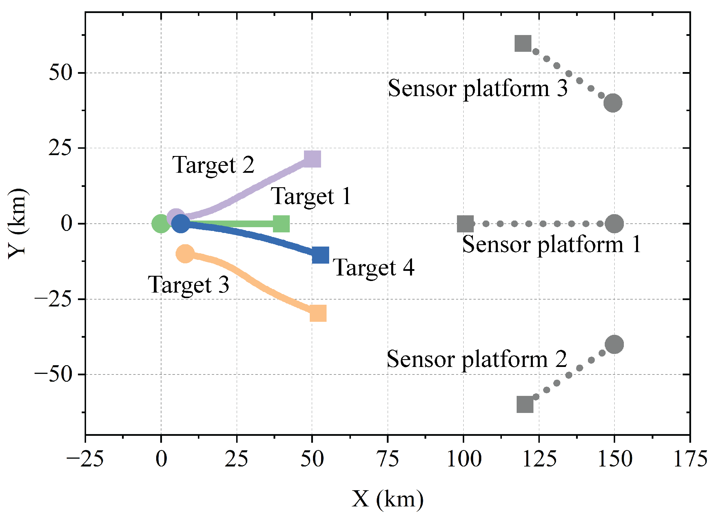
The 2D scenario was assumed to involve three moving sensor platforms and four targets in a network group. The first and second targets were born at $t=1$ s, whereas the third and fourth targets were born at $t=3$ s and $t=5$ s, respectively. The trajectories of the network-group targets and sensor platforms are shown in Figure 5. The false targets intercepted each time were modeled as a Poisson RFS with a Poisson rate of 5. The false target area was $\left[0,55\right]\mathrm{km}\times \left[-32,23\right]\mathrm{km}$, that is, the uniform probability density was $3.3\times {10}^{-10}{\mathrm{m}}^{-2}$. The emission probabilities of the network-group targets were considered to be $P_D=0.7$. When emitting, target 1 had a probability of 0.3 to transmit signals to target 2 and a probability of 0.7 to transmit signals to target 4. Target 2 had a probability of 1 for transmitting signals to target 1. Target 3 had equal probabilities of 0.5 to transmit signals to both targets 1 and 4. Similarly, target 4 also had equal probabilities of 0.5 to transmit signals to both targets 1 and 4. The survival probability of each individual target was independent and was set at $P_S=0.99$. The four thresholds were set as follows: ${\mu }_0={10}^{-3}$, ${\mu }_1=2$, ${\mu }_2=0$, and ${\mu }_3=3$.

Assuming that the network-group target transmitted 258 hopping patterns in one time slot, the signals hopped between 14 frequency points in the range of 969–1008 MHz, 5 frequency points in the range of 1053–1065 MHz, and 32 frequency points in the range of 1113–1206 MHz. The pulse width was 6.4 $\mathsf{\mu }$s and the pulse period was 13 $\mathsf{\mu }$s. The pulse carried 32 bits of data and modulated the carrier wave using MSK at a rate of 5 Mb/s. Each symbol was transmitted in the form of a double pulse, meaning that the two pulses represent the same symbol but with different carrier frequencies. The SNR was 0 dB and the sampling rate was $f_s=10\mathrm{MHz}$. In the pulse sequence, one pulse was selected for signal processing every 11 pulses, resulting in 24 pulses at positions [1, 12, ⋯, 254].

Assuming that there were eight candidate addresses, the addresses for the four targets were 1, 2, 3, and 4. The diagonal elements of the recognizer confusion matrix were 0.9, whereas those of the remaining elements were 0.1/7.

The number of particles was set to 600. In addition, the computational cost could be reduced by using a gating approach. The specific method involved establishing a grid for the TDOAs. In this simulation, because there were three sensor platforms used, a two-dimensional grid was created for the TDOAs. Subsequently, the grid position of each particle at the target density was calculated. Finally, the grid position of the measurement was obtained by calculating the two TDOA values using traditional methods, such as the cross ambiguity function (CAF). If there was an overlap between the grid positions of the particle and measurement, the track and measurement were associated.

Since there is no existing literature on research targeting network groups for comparison, the proposed method was compared with the two-step and noncoherent methods. The two-step method involves using the CAF to jointly estimate the TDOA and Doppler velocity difference and then performing state estimation by incorporating both into the likelihood function. The two-step method, which ignores the inherent constraint that the measurements obtained in the first step must be consistent with the target kinematic state determined in the second step, is suboptimal. The difference between the noncoherent and proposed methods lies in the fact that the former does not consider the term $f_n\frac{\Delta {\dot{d}}_l}{c}(n-1)T_p$ in (20), which ignores the phase shift caused by variations in the frequency of frequency-hopping pulses and time-varying TDOAs. Therefore, it is expected that the proposed method will outperform the other two.

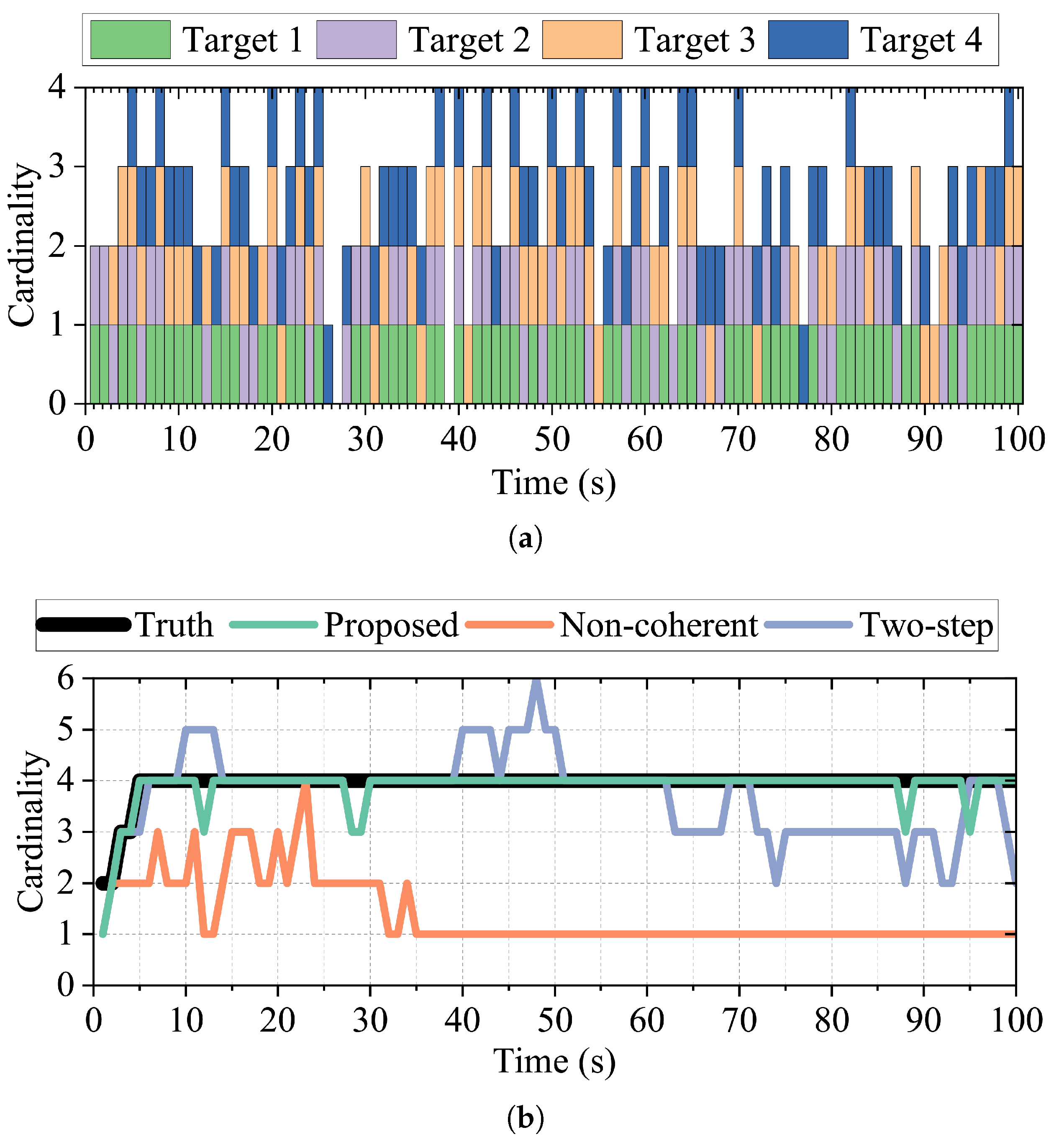
The actual signal emission from the network-group targets in a single simulation varied over time, as depicted in Figure 6a, whereas the cardinality estimation of the three methods in a single simulation is illustrated in Figure 6b. It was evident that the proposed method provided the most accurate cardinality estimation, with only occasional instances of underestimation. The two-step method performed better, whereas the noncoherent method performed the worst, estimating a cardinality of only one after t = 35 s.

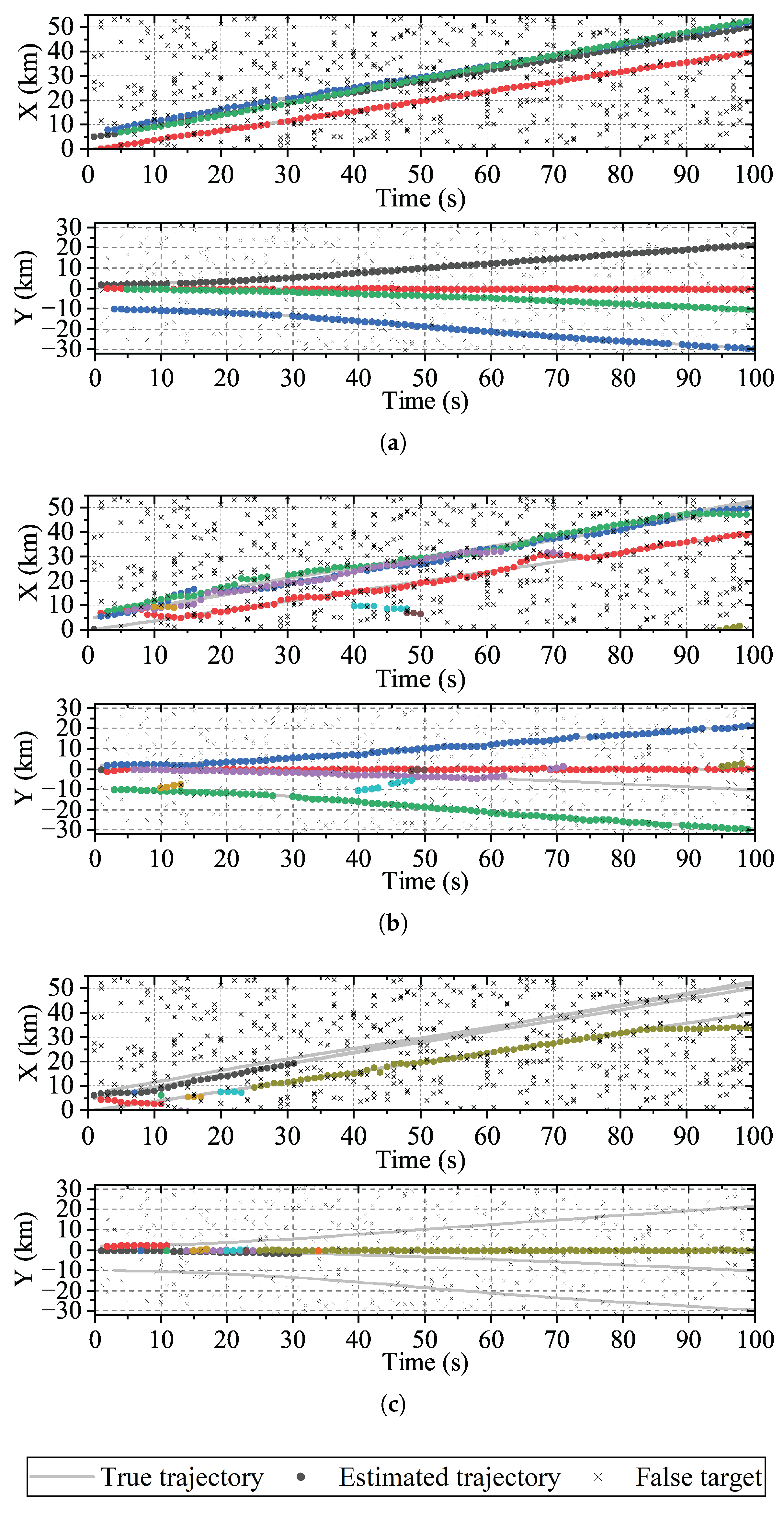
Figure 7 shows the actual and estimated trajectories of the network-group targets in a single simulation, as obtained through (68). From Figure 7a, it is evident that the proposed method accurately estimated the trajectories, but there were occasional instances of missed detections, such as at t = 12 s. By combining Figure 5 and Figure 6a, it is apparent that the missed detection was attributed to target 2, which did not emit multiple times. However, at t = 13 s, the proposed method tracked target 2. The two-step method yielded numerous false trajectories, and the trajectory estimation of target 4 was not detected after t = 63 s. The trajectory estimation performance of the noncoherent method was even worse, with only one target being tracked at t = 100 s.

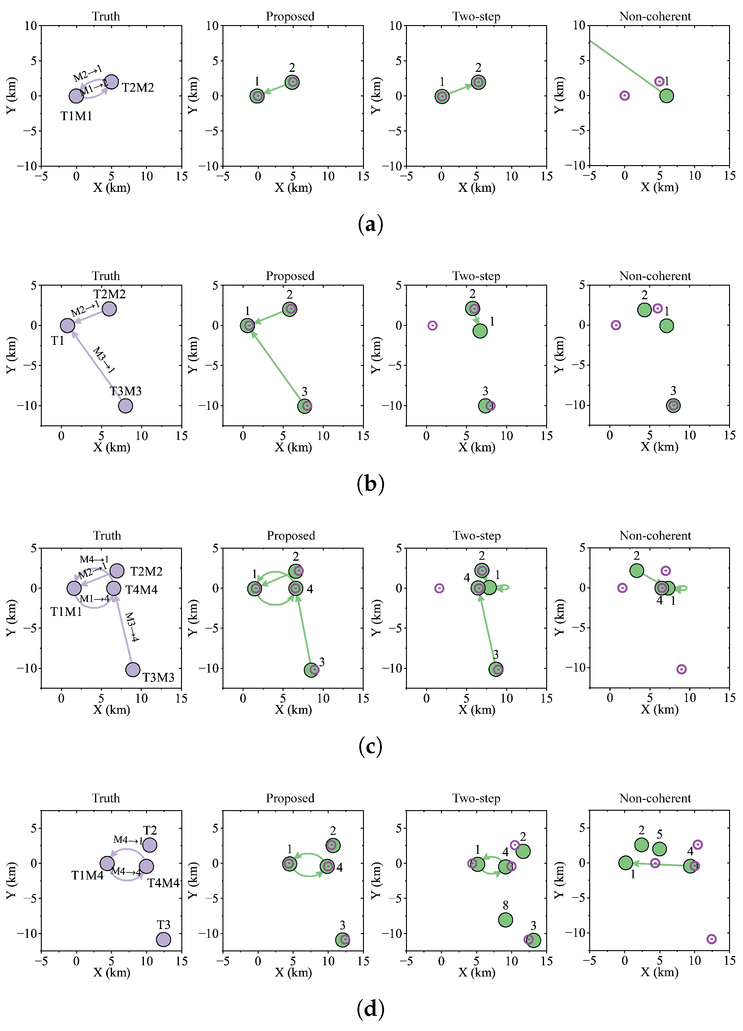
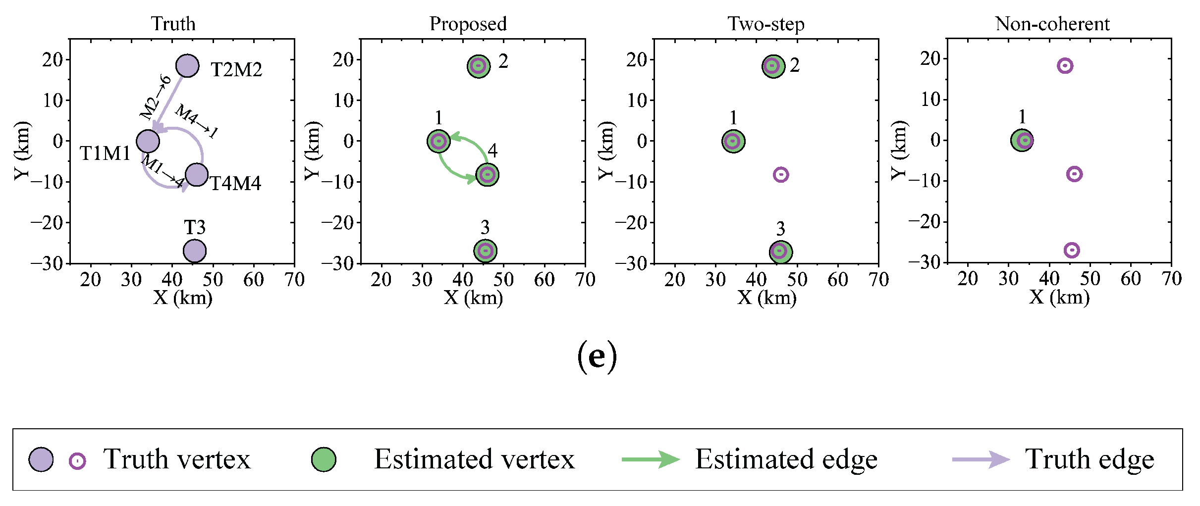
Figure 8 presents comparative network topology estimations from the three different methods within a single simulation trial, as obtained through (69)–(71). The initial graph in each row illustrates the actual network topology, along with the observed measurements, with the caveat that false targets are not marked on the graphs. The subsequent trio of graphs on the right displays the network topology estimations derived by the proposed, two-step, and noncoherent methods. At t = 1 s, both the proposed and two-step methods estimated two vertices in the case of only one target detected; however, only one edge was detected. The noncoherent method detected one target and one edge with the position of the other unknown. At t = 3 s, the proposed method successfully determined the correct network structure. However, the two-step and noncoherent methods had errors in the target position estimation and missed edge estimation. At t = 5 s, the actual and recognized network structures remained congruent. The proposed method identified network connections, whereas the two-step method obtained an incorrect position for the target with address 1 and an incomplete edge estimation. The estimation using the noncoherent method was even worse. At t = 12 s, the system misidentified the address of target 1 as target 4. Despite this error, all the methods managed to accurately assign the correct address number 1 to this target. The two-step method had a poorer position estimation than the proposed method and incorrectly identified a target with address 8. At t = 86 s, the connections from vertex 2 to vertex 1 were mistakenly read as two to six. In this instance, vertex 6 was incorrectly considered a non-existent target; hence, all methods failed to detect the edge 2 → 1. In addition to missing targets, the two-step and noncoherent methods failed to detect edges. It is evident that the estimation of the network topology tended to be accurate when a set of network-group targets could be reliably tracked and there was sufficient information to ascertain their addresses. However, disruptions or errors in target trajectories could lead to inaccuracies in the assessment of the network topology.

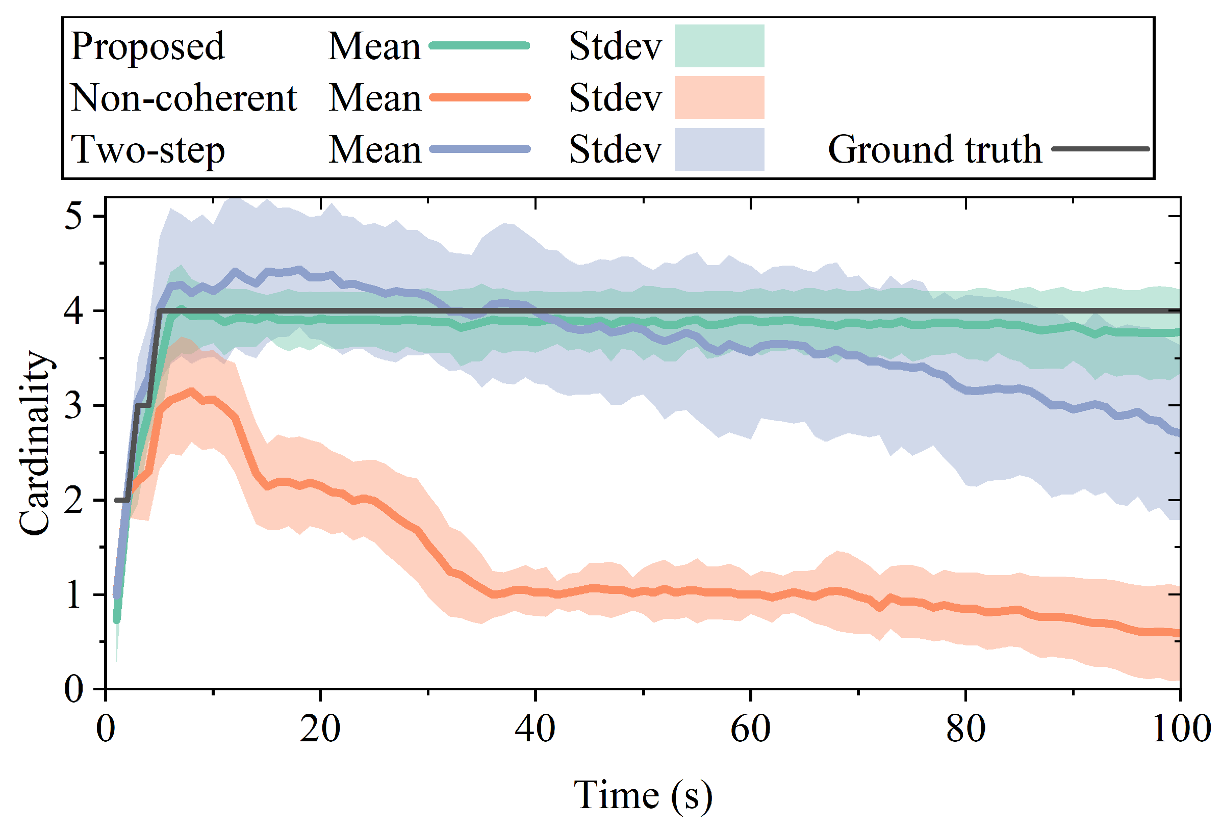
A performance comparison was conducted through 100 Monte Carlo simulations in Figure 9, Figure 10 and Figure 11. Figure 9 compares the cardinality estimation performances of the three methods. The proposed method provided the most accurate cardinality estimation, whereas the other two methods tended to underestimate the cardinality. This was because with a limited number of particles, the tracked targets in these methods could experience track loss or interruption, making it difficult to maintain stable tracking.

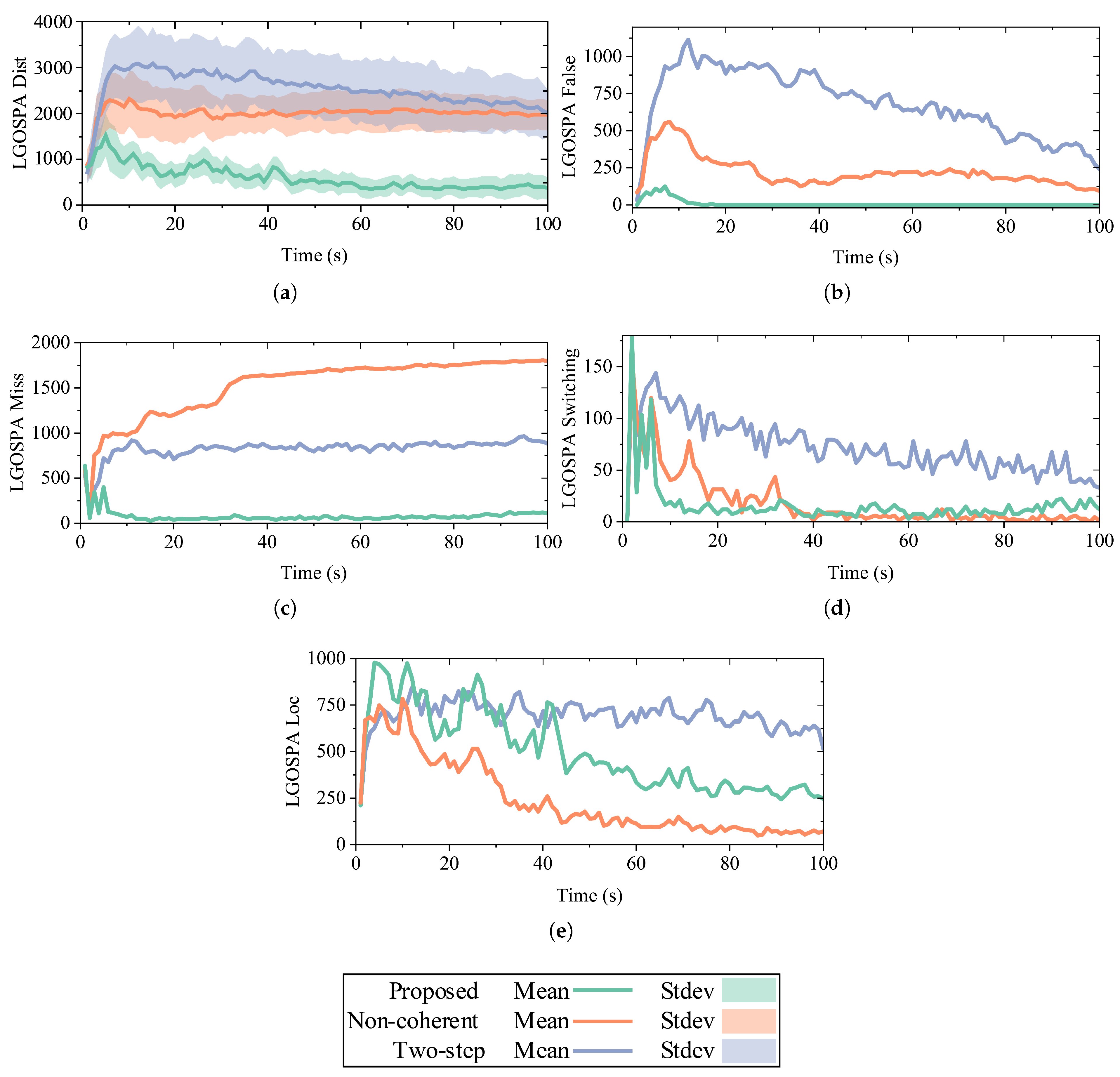
The labeled generalized optimal sub-pattern assignment (LGOSPA) error was utilized to evaluate the performance of the tracking methods. It decomposed the error into four components: the target localization error, missed target, false alarm target, and track switches. The relationship between the LGOSPA and GOSPA is given by the following equation:

$$LGOSPA={\left(GOSP{A}^p+S{C}^p\right)}^{\frac{1}{p}}$$

(74)

where p is the metric order, $SC=SP\times n_s^{1/p}$ is the switching component, $SP$ is the switching penalty, and $n_s$ is the number of switches. The GOSPA can be found in the study conducted by Abu et al. [45]. In the simulation, we set $SP=300$, $p=1$, the cutoff distance to 1000, and the alpha parameter to 2. Figure 10 shows a comparison of the LGOSPA errors and their components for the three methods. From Figure 10a, it can be observed that the proposed method had the lowest mean and smallest variance of the LGOSPA distance between the three methods, followed by the noncoherent and two-step methods. The proposed method exhibited the lowest false component within the LGOSPA metric, achieving a value of zero at t = 18 s, which signified the absence of false tracks. In contrast, the two-step method demonstrated a marked inferior performance relative to the proposed method, with higher false and switching components. The noncoherent method incurred the greatest miss component. However, as shown in Figure 10e, the performance of the incoherent method was lower than that of the proposed method because of the missed detections. Overall, the proposed method outperformed the other methods.

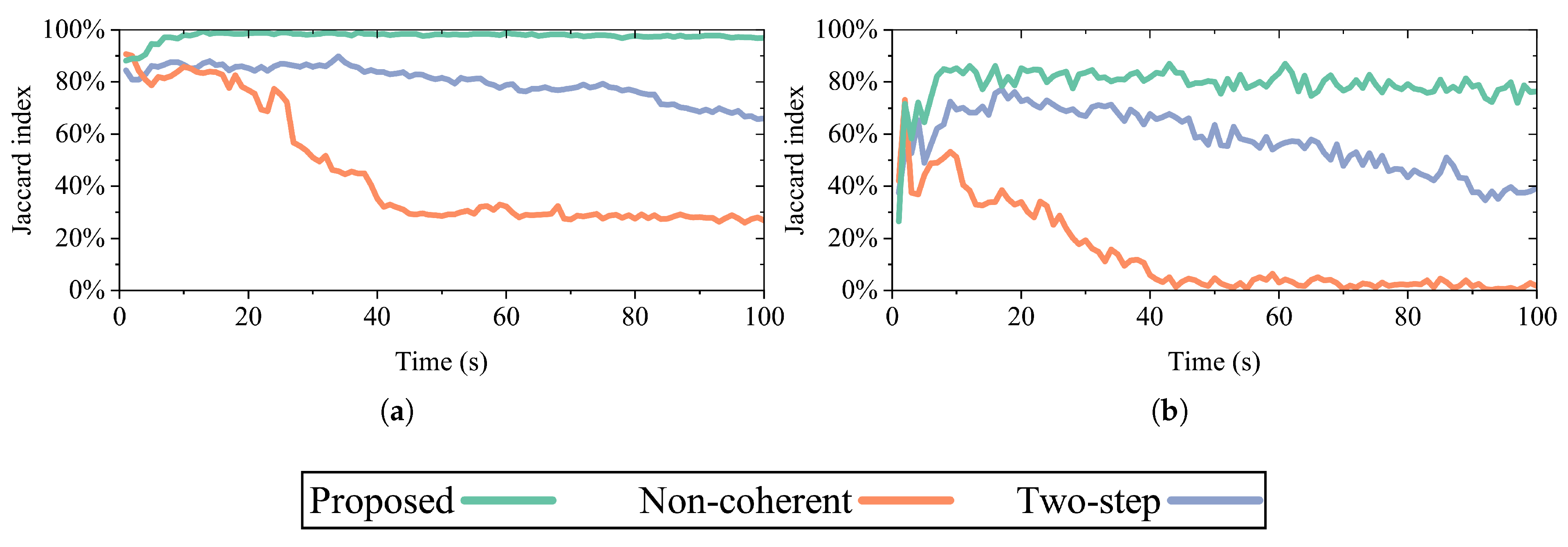
The Jaccard similarity measures the similarity and dissimilarity between finite sets using the Jaccard index. The higher the Jaccard index value, the higher the similarity between the samples. The Jaccard index is calculated as follows:

$$J\left(A,B\right)=\frac{\left|A\cap B\right|}{\left|A\cup B\right|}$$

(75)

Figure 11 shows the performance of the vertex and edge estimation, which represents the estimation performance of the addresses and the links in the network topology, respectively. In Figure 11a, it can be observed that the estimation performance of the proposed method gradually improved before t = 13 s owing to the accumulation of address information. Ultimately, only the proposed method maintained a high level of accuracy, whereas the performances of the other two methods declined. As illustrated in Figure 11b, our method stabilized at approximately 80% accuracy in the estimation of opposite edges after t = 8 s, outperforming the two-step approach. Beyond t = 44 s, the incoherent method was almost incapable of obtaining correct edge estimations.

7. Conclusions

This study considered the state and network topology estimations of network-group targets. In contrast to previous studies, the focus was on several aspects. Initially, the modeling was based on an LMB random finite set. Subsequently, the measurement likelihood function was directly incorporated into network-group target communication signals, which contained Doppler and time-delay information. Finally, by combining this with graph theory, the network-group target network topology structure was estimated. The simulation results validated the effectiveness of the method for estimating both parameters.

However, this study was limited in its ability to estimate the network topology structure at each time step. Future work may involve estimating the state and network topology within the RFS framework, considering the constraints of the network and physical spaces. This study employed fixed time steps for prediction and updates. However, when the probability of network-group targets emitting signals are exceedingly low, or when the signal emission adheres to a specific pattern, leading to a near absence of target signals within time slots close to fixed time steps, it becomes necessary to consider non-uniform time intervals. Additionally, extending this method to 3D scenarios in a close-range scenario can also one of the future works.

References

1. Zhou, L.; Leng, S.; Liu, Q.; Wang, Q. Intelligent UAV swarm cooperation for multiple targets tracking. IEEE Internet Things J. 2021, 9, 743–754. [Google Scholar] [CrossRef]
2. Hayat, S.; Yanmaz, E.; Muzaffar, R. Survey on unmanned aerial vehicle networks for civil applications: A communications viewpoint. IEEE Commun. Surv. Tutor. 2016, 18, 2624–2661. [Google Scholar] [CrossRef]
3. Jinqiang, H.; Husheng, W.; Renjun, Z.; Rafik, M.; Xuanwu, Z. Self-organized search-attack mission planning for UAV swarm based on wolf pack hunting behavior. J. Syst. Eng. Electron. 2021, 32, 1463–1476. [Google Scholar] [CrossRef]
4. Huo, M.; Duan, H.; Zeng, Z. Cluster Space Control Method of Manned-Unmanned Aerial Team for Target Search Task. IEEE Trans. Circuits Syst. II Express Briefs 2023, 70, 2545–2549. [Google Scholar] [CrossRef]
5. Kalman, R.E. A new approach to linear filtering and prediction problems. J. Basic Eng. 1960, 82, 35–45. [Google Scholar] [CrossRef]
6. Julier, S.J.; Uhlmann, J.K. Unscented filtering and nonlinear estimation. Proc. IEEE 2004, 92, 401–422. [Google Scholar] [CrossRef]
7. Bar-Shalom, Y.; Fortmann, T.E.; Cable, P.G. Tracking and data association. J. Acoust. Soc. Am. 1990, 87, 918–919. [Google Scholar] [CrossRef]
8. Wang, S.; Bao, Q. Single target tracking for noncooperative bistatic radar with unknown signal illumination. Signal Process. 2021, 183, 107991. [Google Scholar] [CrossRef]
9. Guizhou, W.; Zhang, M.; Chaoxin, H.; Fucheng, G. Direct position determination using single moving rotating linear array: Noncoherent and coherent processing. Chin. J. Aeronaut. 2020, 33, 688–700. [Google Scholar]
10. Sidi, A.Y.; Weiss, A.J. Delay and Doppler induced direct tracking by particle filter. IEEE Trans. Aerosp. Electron. Syst. 2014, 50, 559–572. [Google Scholar] [CrossRef]
11. Guo, Y.; Yang, J.; Tang, Q.; Li, W.C. Direct Localization Algorithm of Moving Target for Passive Radar. In Proceedings of the 2018 15th International Computer Conference on Wavelet Active Media Technology and Information Processing (ICCWAMTIP), Chengdu, China, 14–16 December 2018; pp. 89–92. [Google Scholar]
12. Ma, F.; Guo, F.; Yang, L. Direct position determination of moving sources based on delay and Doppler. IEEE Sens. J. 2020, 20, 7859–7869. [Google Scholar] [CrossRef]
13. Wang, D.; Yin, J.; Yu, H. DPD algorithm for moving source based on Doppler frequency shifts: Case of known waveforms. Chin. J. Electron. 2019, 28, 978–986. [Google Scholar] [CrossRef]
14. Xia, N.; Li, B.; Wang, J. Direct tracking of co-channel moving sources with different cyclic frequencies. IEEE Commun. Lett. 2020, 24, 1715–1718. [Google Scholar] [CrossRef]
15. Yu, W.; Yu, H.; Du, J.; Zhang, M.; Wang, D. A deep learning algorithm for joint direct tracking and classification of manoeuvring sources. IET Radar Sonar Navig. 2022, 16, 1198–1211. [Google Scholar] [CrossRef]
16. Blackman, S.S. Multiple hypothesis tracking for multiple target tracking. IEEE Aerosp. Electron. Syst. Mag. 2004, 19, 5–18. [Google Scholar] [CrossRef]
17. Musicki, D.; Evans, R. Joint integrated probabilistic data association: JIPDA. IEEE Trans. Aerosp. Electron. Syst. 2004, 40, 1093–1099. [Google Scholar] [CrossRef]
18. Tian, Y.; Liu, M.; Zhang, S.; Zheng, R.; Fan, Z. Feature-Aided Passive Tracking of Noncooperative Multiple Targets Based on the Underwater Sensor Networks. IEEE Internet Things J. 2022, 10, 4579–4591. [Google Scholar] [CrossRef]
19. Mahler, R. Statistical Multisource-Multitarget Information Fusion; Artech: Morristown, NJ, USA, 2007. [Google Scholar]
20. Mahler, R.P. Advances in Statistical Multisource-Multitarget Information Fusion; Artech House: Norwood, MA, USA, 2014. [Google Scholar]
21. Zhenzhen, S.; Hongbing, J.; Cong, T.; Zhang, Y. A robust Poisson multi-Bernoulli filter for multi-target tracking based on arithmetic average fusion. Chin. J. Aeronaut. 2023, 36, 179–190. [Google Scholar]
22. Zeng, H.; Chen, J.; Wang, P.; Liu, W.; Zhou, X.; Yang, W. Moving target detection in multi-static GNSS-Based passive radar based on multi-Bernoulli filter. Remote Sens. 2020, 12, 3495. [Google Scholar] [CrossRef]
23. Cao, C.; Zhao, Y. A Multi-Frame GLMB Smoothing Based on the Image-Observation Sensor for Tracking Multiple Weak Targets Using Belief Propagation. Remote Sens. 2022, 14, 5666. [Google Scholar] [CrossRef]
24. Koch, J.W. Bayesian approach to extended object and cluster tracking using random matrices. IEEE Trans. Aerosp. Electron. Syst. 2008, 44, 1042–1059. [Google Scholar] [CrossRef]
25. Granstrom, K.; Orguner, U. A PHD filter for tracking multiple extended targets using random matrices. IEEE Trans. Signal Process. 2012, 60, 5657–5671. [Google Scholar] [CrossRef]
26. Granström, K.; Natale, A.; Braca, P.; Ludeno, G.; Serafino, F. Gamma Gaussian inverse Wishart probability hypothesis density for extended target tracking using X-band marine radar data. IEEE Trans. Geosci. Remote Sens. 2015, 53, 6617–6631. [Google Scholar] [CrossRef]
27. Li, Y.; Wei, P.; Li, G.; Chen, Y.; Gao, L.; Zhang, H. Joint detection, tracking and classification of multiple extended objects based on the JDTC-GIW-MeMBer filter. Signal Process. 2021, 178, 107800. [Google Scholar] [CrossRef]
28. Mihaylova, L.; Carmi, A.Y.; Septier, F.; Gning, A.; Pang, S.K.; Godsill, S. Overview of Bayesian sequential Monte Carlo methods for group and extended object tracking. Digit. Signal Process. 2014, 25, 1–16. [Google Scholar] [CrossRef]
29. Zhejun, L.; Weidong, H. Estimation of ballistic coefficients of space debris using the ratios between different objects. Chin. J. Aeronaut. 2017, 30, 1204–1216. [Google Scholar]
30. Pang, S.K.; Li, J.; Godsill, S.J. Detection and tracking of coordinated groups. IEEE Trans. Aerosp. Electron. Syst. 2011, 47, 472–502. [Google Scholar] [CrossRef]
31. Khan, Z.; Balch, T.; Dellaert, F. MCMC-based particle filtering for tracking a variable number of interacting targets. IEEE Trans. Pattern Anal. Mach. Intell. 2005, 27, 1805–1819. [Google Scholar] [CrossRef] [PubMed]
32. Gning, A.; Mihaylova, L.; Maskell, S.; Pang, S.K.; Godsill, S. Group object structure and state estimation with evolving networks and Monte Carlo methods. IEEE Trans. Signal Process. 2010, 59, 1383–1396. [Google Scholar] [CrossRef]
33. Zhang, Z.; Sun, J.; Zhou, H.; Xu, C. Group target tracking based on MS-MeMBer filters. Remote Sens. 2021, 13, 1920. [Google Scholar] [CrossRef]
34. Chen, X.; Qin, Z.; An, L.; Bhanu, B. Multiperson tracking by online learned grouping model with nonlinear motion context. IEEE Trans. Circuits Syst. Video Technol. 2015, 26, 2226–2239. [Google Scholar] [CrossRef]
35. Cheng, X.; Song, L.; Zou, Z. Multiple group target tracking with evolving networks and labeled box particle PHD filter. In Proceedings of the 2018 Chinese Control And Decision Conference (CCDC), Shenyang, China, 9–11 June 2018; pp. 4046–4051. [Google Scholar]
36. Liu, W.; Zhu, S.; Wen, C.; Yu, Y. Structure modeling and estimation of multiple resolvable group targets via graph theory and multi-Bernoulli filter. Automatica 2018, 89, 274–289. [Google Scholar] [CrossRef]
37. Yu, H.; An, W.; Zhu, R.; Guo, R. A hypergraph matching labeled multi-Bernoulli filter for group targets tracking. IEICE Trans. Inf. Syst. 2019, 102, 2077–2081. [Google Scholar] [CrossRef]
38. Hao, X.; Liang, Y.; Zhang, W.; Xu, L. Structure identification and tracking of multiple resolvable group targets with circular formation. In Proceedings of the 2020 IEEE 9th Joint International Information Technology and Artificial Intelligence Conference (ITAIC), Chongqing, China, 11–13 December 2020; Volume 9, pp. 910–915. [Google Scholar]
39. Zhao, Z.; Liu, W.; Wang, S.; Gao, S. Large-batch and multi-structure group targets tracking based on serial glmb. In Proceedings of the 2021 International Conference on Control, Automation and Information Sciences (ICCAIS), Xi’an, China, 14–17 October 2021; pp. 949–954. [Google Scholar]
40. Li, G.; Li, G.; He, Y. Resolvable group target tracking via multi-Bernoulli filter and its application to sensor control scenario. IEEE Trans. Signal Process. 2022, 70, 6286–6299. [Google Scholar] [CrossRef]
41. Badshah, F.; Shah, S.T.U.; Jan, S.R.; Rahman, I.U. Communication between multiple processes on same device using TCP/IP suite. In Proceedings of the 2017 International Conference on Communication, Computing and Digital Systems (C-CODE), Islamabad, Pakistan, 8–9 March 2017; pp. 148–151. [Google Scholar]
42. West, D.B. Introduction to Graph Theory; Prentice Hall: Hoboken, NJ, USA, 2001; Volume 2. [Google Scholar]
43. Skarding, J.; Gabrys, B.; Musial, K. Foundations and modeling of dynamic networks using dynamic graph neural networks: A survey. IEEE Access 2021, 9, 79143–79168. [Google Scholar] [CrossRef]
44. Reuter, S.; Vo, B.T.; Vo, B.N.; Dietmayer, K. The labeled multi-Bernoulli filter. IEEE Trans. Signal Process. 2014, 62, 3246–3260. [Google Scholar]
45. Rahmathullah, A.S.; García-Fernández, Á.F.; Svensson, L. Generalized optimal sub-pattern assignment metric. In Proceedings of the 2017 20th International Conference on Information Fusion (Fusion), Xi’an, China, 10–13 July 2017; pp. 1–8. [Google Scholar]
Figure 1. Time slot diagram of a network-group target. Network-group targets transmit information within a given time slot, as represented by solid patterns when transmitting and hollow patterns otherwise. The straight black arrow beside the pattern indicates the direction of movement of the target in the slot. The example of frequency-hopping patterns for signal transmission is shown above.
Remotesensing 16 01275 g001
Figure 2. The intercepted network-group target time slot diagram is shown with N s = 4 .
Remotesensing 16 01275 g002
Figure 3. Sequence diagrams for the transmitter and receiver. The signal transmission direction is indicated by a blue lightning symbol. (a) Ground truth. (b) After recognition.
Remotesensing 16 01275 g003
Figure 4. The flowchart of the proposed tracking method.
Remotesensing 16 01275 g004
Figure 5. Simulation scenery in an X–Y coordinate system, where the solid lines represent the trajectory of the network-group targets, the dotted lines represent the trajectories of the sensor platforms, and the start/stop points for each trajectory are shown with a solid circle/square.
Remotesensing 16 01275 g005
Figure 6. (a) The emitting of the targets. (b) The cardinality estimation in a single simulation.
Remotesensing 16 01275 g006
Figure 7. True trajectories of the network-group targets and estimated trajectories in a single simulation. (a) The proposed method. (b) The two-step method. (c) The noncoherent method.
Remotesensing 16 01275 g007
Figure 8. Network topology estimation of three methods in a single simulation. ”TaMb” represents a true address of a and the measurement was b. “Ta” indicates that the actual address was a and the target was silent. “M c d ” represents the transmitter address measurement and receiver addresses were c and d, respectively. Edges without arrows indicate that the position of the receiver was unknown. (a) t = 1 s. (b) t = 3 s. (c) t = 5 s. (d) t = 12 s. (e) t = 86 s.
Remotesensing 16 01275 g008aRemotesensing 16 01275 g008b
Figure 9. Comparison of cardinality estimation performance for three methods.
Remotesensing 16 01275 g009
Figure 10. Comparison of the LGOSPA distance and its components for three methods. (a) LGOSPA distance. (b) LGOSPA false target component. (c) LGOSPA missed target component. (d) LGOSPA switching component. (e) LGOSPA localization component.
Remotesensing 16 01275 g010
Figure 11. Comparison of Jaccard similarity coefficients for three methods. (a) Vertices. (b) Edges.
Remotesensing 16 01275 g011
Disclaimer/Publisher’s Note: The statements, opinions and data contained in all publications are solely those of the individual author(s) and contributor(s) and not of MDPI and/or the editor(s). MDPI and/or the editor(s) disclaim responsibility for any injury to people or property resulting from any ideas, methods, instructions or products referred to in the content.