
High-Resolution Canopy Height Mapping: Integrating NASA’s Global Ecosystem Dynamics Investigation (GEDI) with Multi-Source Remote Sensing Data
 , ,
, ,  , ,
, ,  ,
,  , ,
, ,  and
and
Abstract
:1. Introduction

| Site | Year | Methods | Dependent Variables | Independent Variables | Map Accuracy | Study | |
|---|---|---|---|---|---|---|---|
| Output Pixel-Based | Statistic Measurements | ||||||
| Global map | 2000–2017 | NA | ICESat | LDT | 30 m | MAE = 3.7 m; R-squared = 0.85–0.92 | [31] |
| China’s forest | 2017–2019 | DL and RF | ICESat-2 | S1, S2 and LDT8 | 10 m−30 m−250 m−500 m−1000 m | R-squared = 0.68−0.78; bias = −1.46 m | [29] |
| USA | 2019–2021 | RF | GEDI | S1 and S2 | 30 m | r = 0.58; RMSE = 4.46 m | [32] |
| Canada | 2019 | LM (i.e., OLS) | ICESat-2 | NTEMS (validation) | 100 m segments | r = 0.61; mean difference = 0.55 m | [8] |
| Global map | April–October 2019 | RF | GEDI | LDT | 30 m | RMSE = 6.6 m; MAE = 4.45 m, R-squared = 0.62 | [27] |
| China, France, and the United States | 2019 | RF | GEDI | S2 | 10 m | OA China = 0.89; OA France = 0.85; OA US = 0.91 | [26] |
| Global map | 2020 | DL (I.e., CNN) | GEDI | S2 | 10 m | RMSE = 9.6 m; MAE = 7.4 m; ME = −4.8 m | [28] |
| Australia and the United States | 2020 | GB | GEDI | S1 and S2 | 100 m–200 m | R-squared of 0.66–0.74; RMSE of 41–77% | [25] |
- (1)
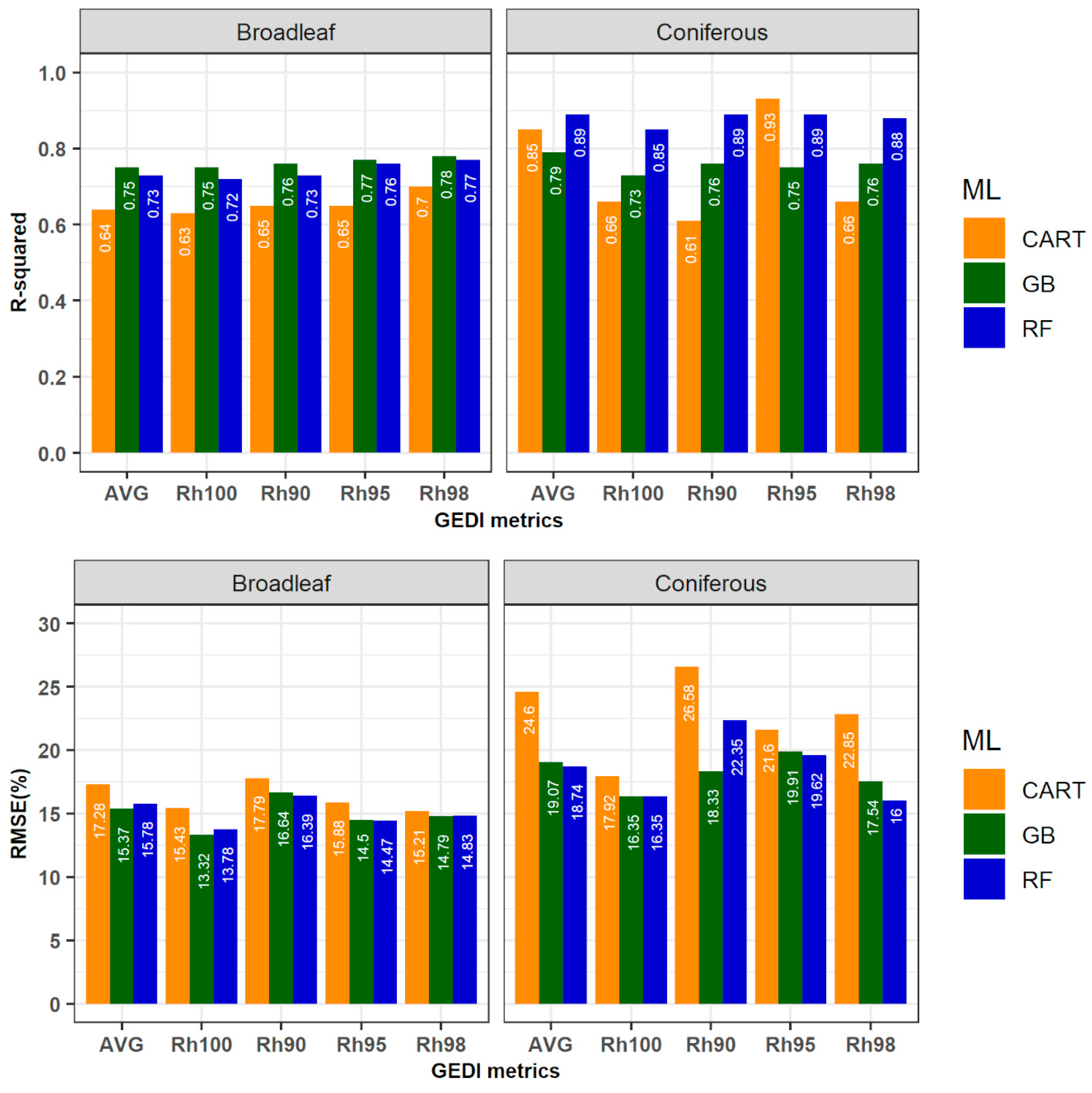
- To assess the performance of three ML algorithms, RF, GB, and CART, in predicting canopy heights from the most commonly used GEDI metrics.
- (2)
- To evaluate the performance of our canopy height maps using reference ALS-based CHMs.
- (3)
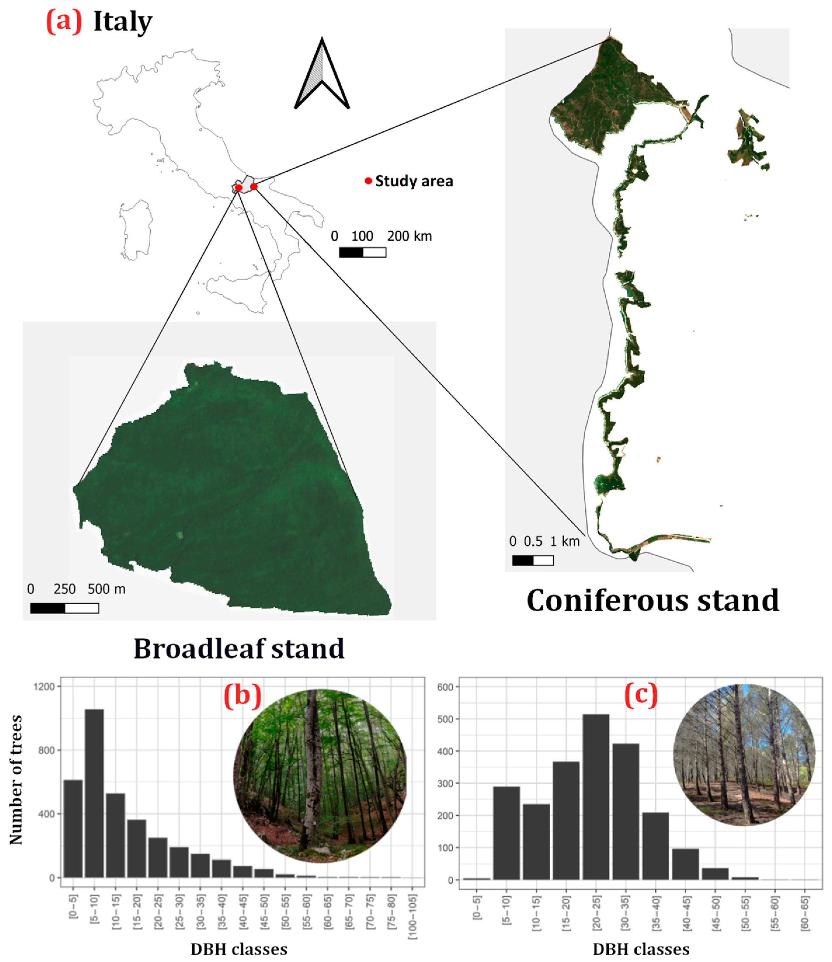
2. Study Area
3. Data
3.1. Airborne Laser Scanning Data Collection and Processing
3.2. Global Ecosystem Dynamics Investigation (GEDI) Level-2A Data
3.3. Sentinel Mission Data
3.4. Topographical Data
3.5. Existing Global Ecosystem Dynamics Investigation (GEDI)-Derived Canopy Height Maps
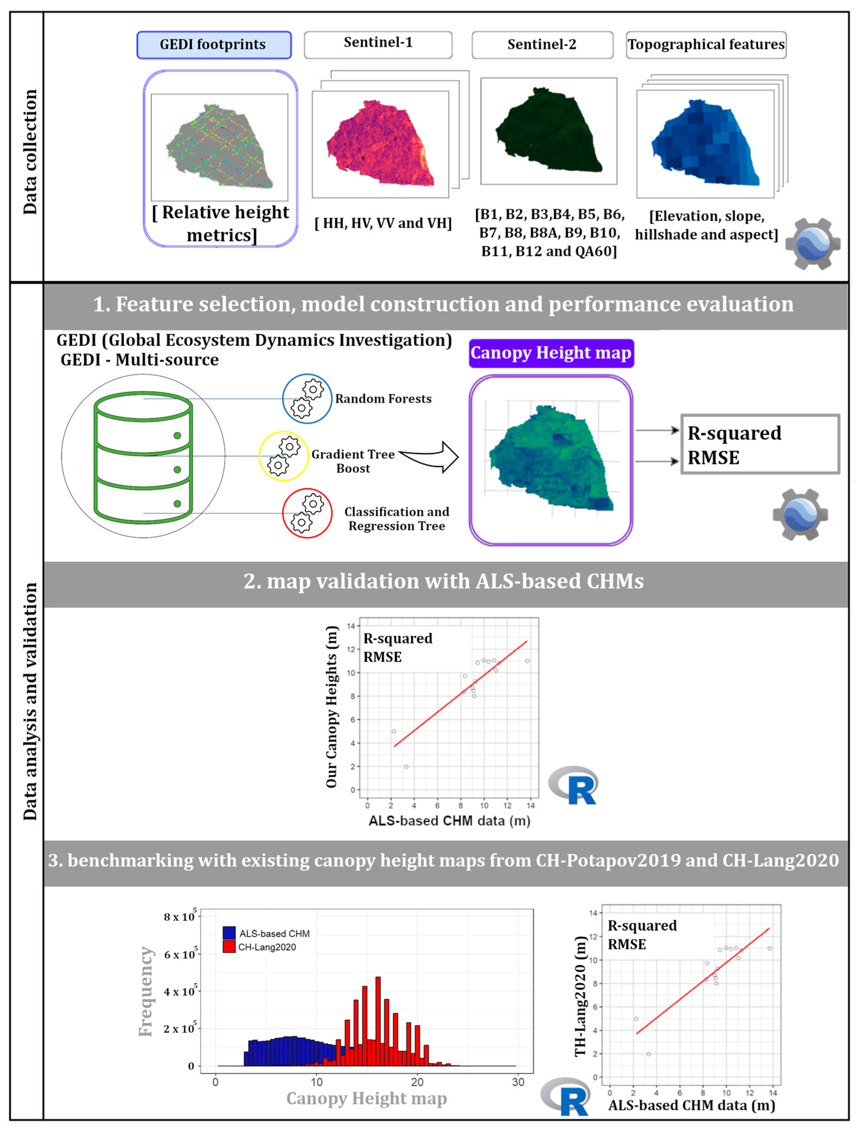
4. Methods
4.1. Canopy Height Map Prediction
4.2. Comparison of Predicted Canopy Height Maps with Reference Airborne Laser Scanning (ALS)-Based Canopy Height Models (CHMs)
4.3. Comparison of Predicted Canopy Height Maps with Other Existing Global Ecosystem Dynamics Investigation (GEDI)-Derived Canopy Height Maps
5. Results
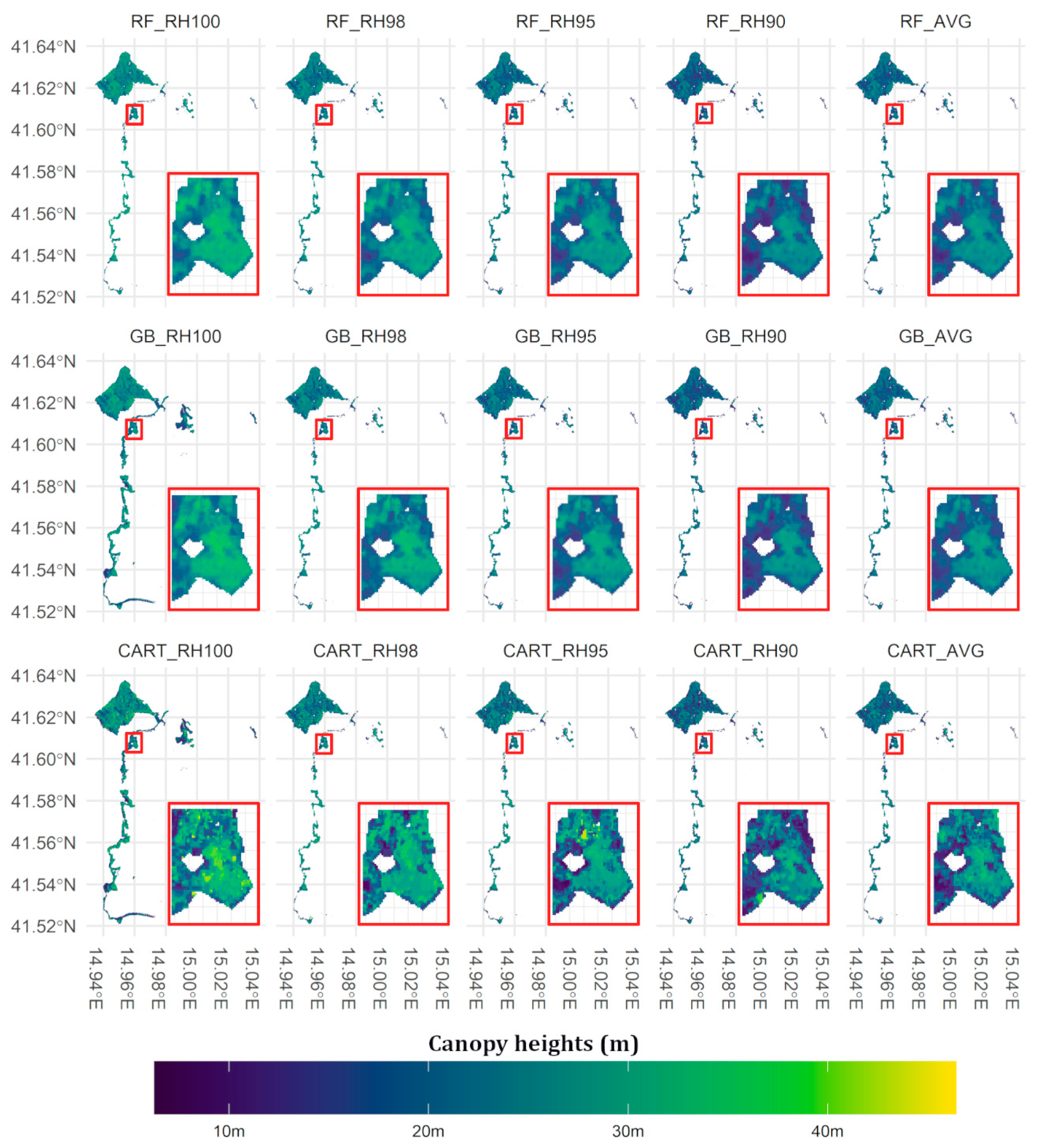
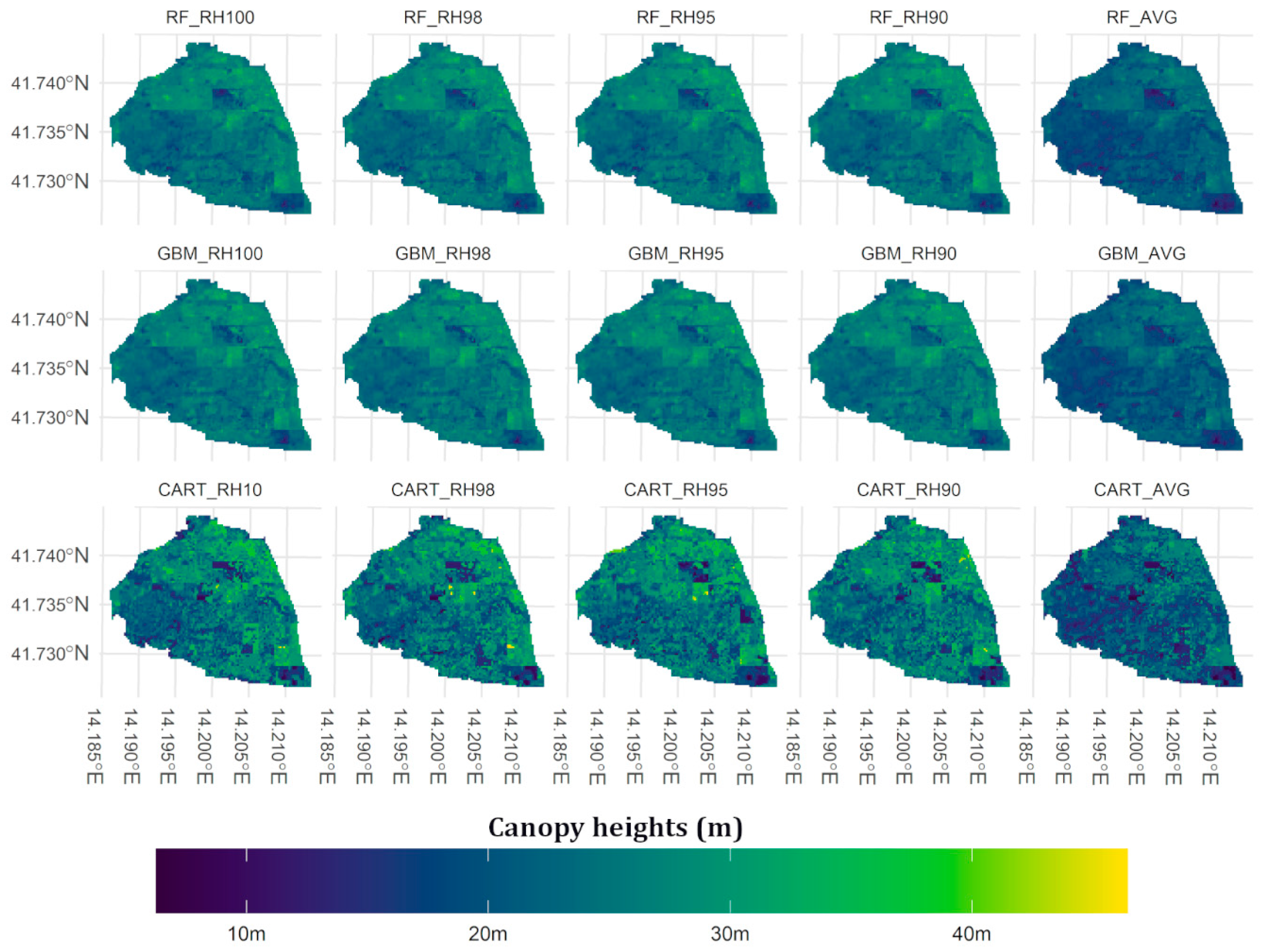
5.1. Canopy Heights Map Prediction
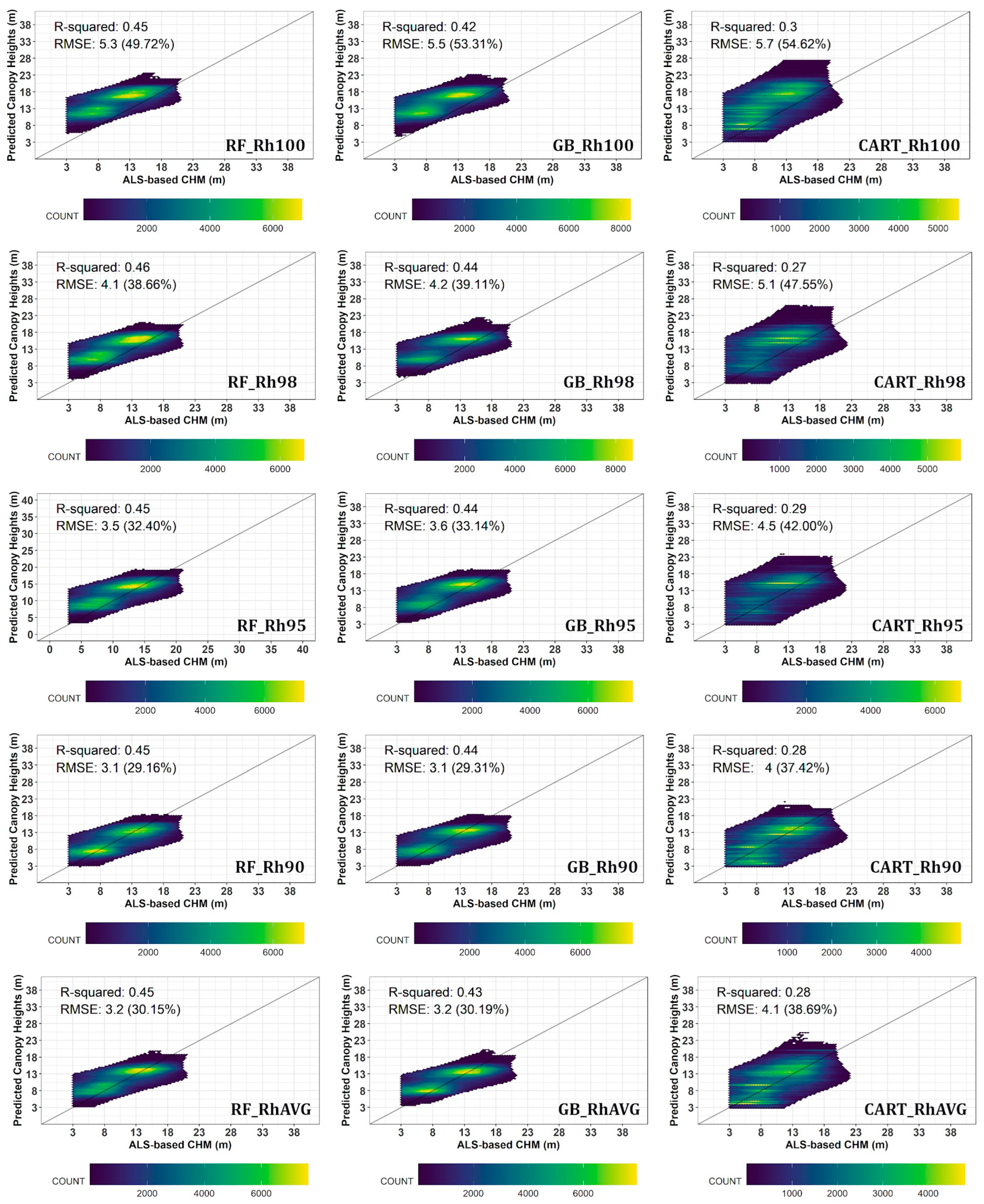
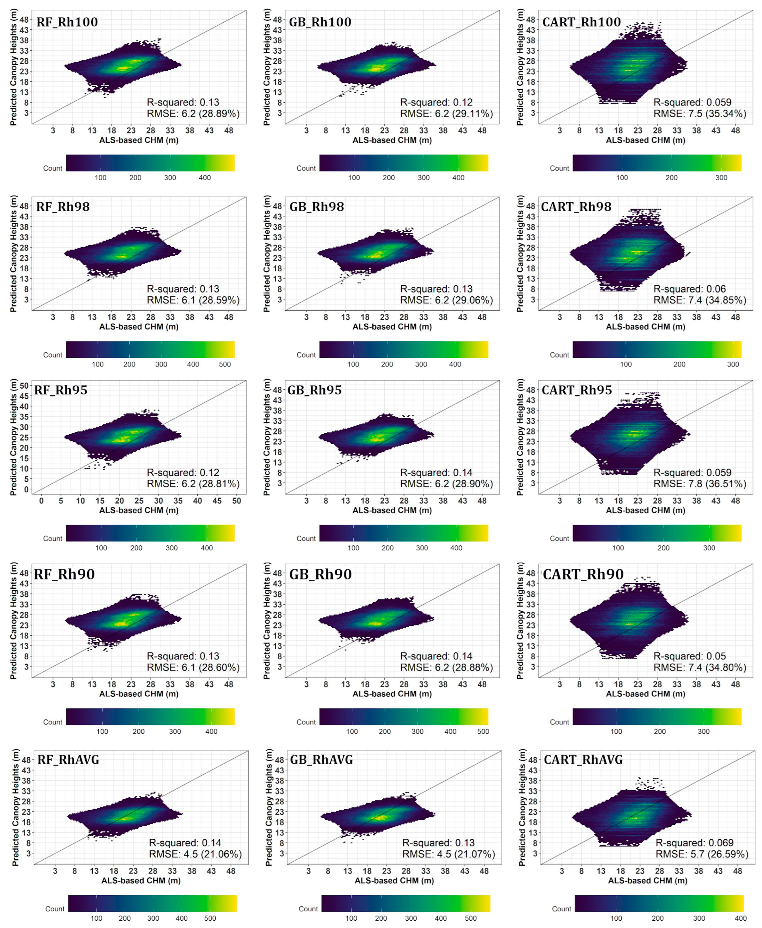
5.2. Comparison of Predicted Canopy Height Map with Reference Airborne Laser Scanning-Based Canopy Height Models
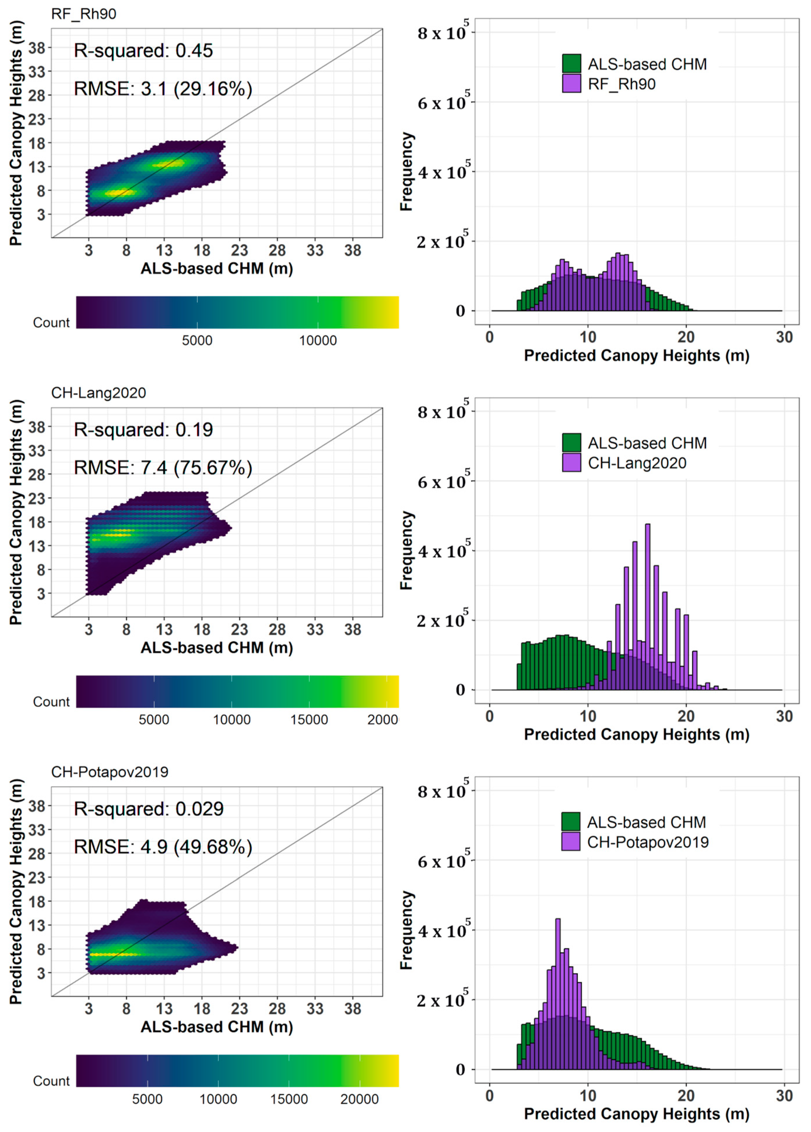
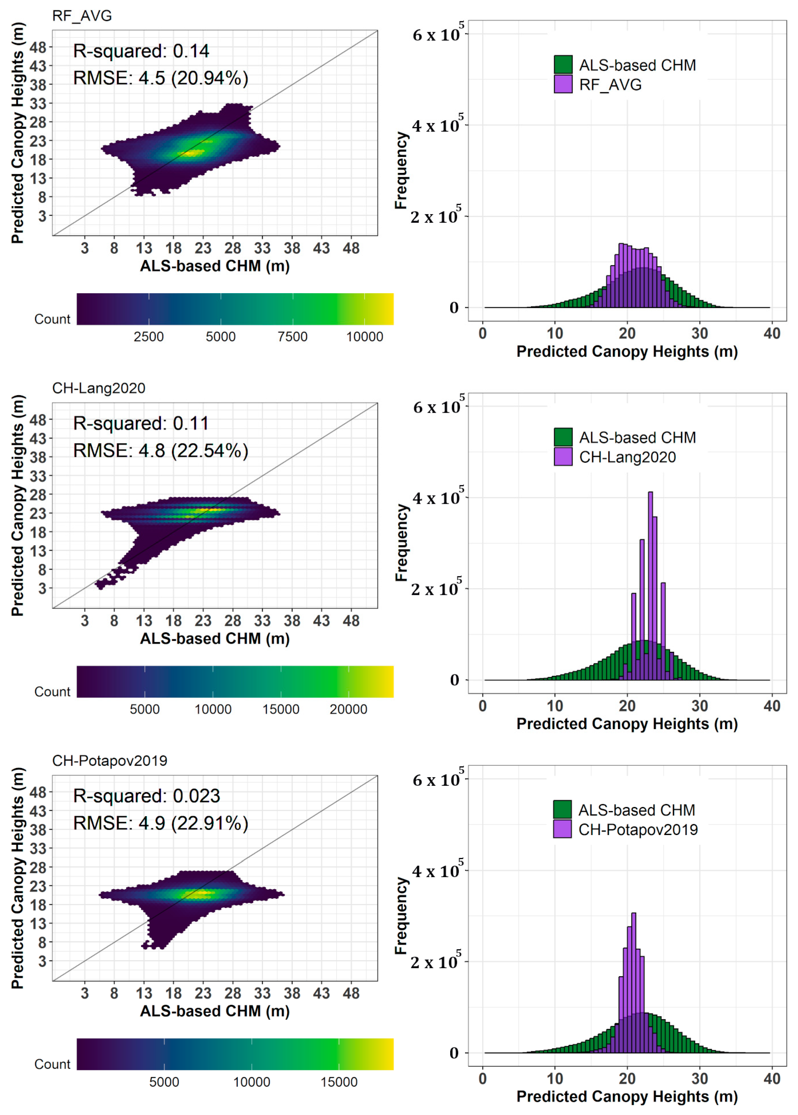
5.3. Comparison of Predicted Canopy Height Maps with Other Existing Global Ecosystem Dynamics Investigation (GEDI)-Derived Canopy Height Maps
6. Discussion
6.1. Canopy Heights Map Prediction
6.2. Comparison of Predicted Canopy Height Maps with Reference Airborne Laser Scanning (ALS)-Based Canopy Height Model Results
6.3. Comparison of Predicted Canopy Height Maps with Other Existing Canopy Height Maps
7. Conclusions
Supplementary Materials
Author Contributions
Funding
Data Availability Statement
Acknowledgments
Conflicts of Interest
References
- Bastin, J.-F.; Finegold, Y.; Garcia, C.; Mollicone, D.; Rezende, M.; Routh, D.; Zohner, C.M.; Crowther, T.W. The Global Tree Restoration Potential. Science 2019, 365, 76–79. [Google Scholar] [CrossRef] [PubMed]
- R. State of Europe Forests. Summary for Policy Markers State of Europe’s Forest 2020. In Proceedings of the Ministerial Conference on the Protection of Forests in Europe, Bratislava, Slovakia, 14–15 April 2020; Liasion Unit Bratislava: Bratislava, Slovakia, 2020; Volume 4, pp. 64–75.
- Brosofske, K.D.; Froese, R.E.; Falkowski, M.J.; Banskota, A. A Review of Methods for Mapping and Prediction of Inventory Attributes for Operational Forest Management. For. Sci. 2014, 60, 733–756. [Google Scholar] [CrossRef]
- Mcroberts, R.; Tomppo, E. Remote Sensing Support for National Forest Inventories. Remote Sens. Environ. 2007, 110, 412–419. [Google Scholar] [CrossRef]
- McRoberts, R.E.; Naesset, E.; Gobakken, T. Accuracy and Precision for Remote Sensing Applications of Nonlinear Model-Based Inference. IEEE J. Sel. Top. Appl. Earth Obs. Remote Sens. 2013, 6, 27–34. [Google Scholar] [CrossRef]
- Vizzarri, M.; Chiavetta, U.; Santopuoli, G.; Tonti, D.; Marchetti, M. Mapping Forest Ecosystem Functions for Landscape Planning in a Mountain Natura2000 Site, Central Italy. J. Environ. Plan. Manag. 2015, 58, 1454–1478. [Google Scholar] [CrossRef]
- Proietti, R.; Antonucci, S.; Monteverdi, M.C.; Garfì, V.; Marchetti, M.; Plutino, M.; Di Carlo, M.; Germani, A.; Santopuoli, G.; Castaldi, C.; et al. Monitoring Spring Phenology in Mediterranean Beech Populations through in Situ Observation and Synthetic Aperture Radar Methods. Remote Sens. Environ. 2020, 248, 111978. [Google Scholar] [CrossRef]
- Mulverhill, C.; Coops, N.C.; Hermosilla, T.; White, J.C.; Wulder, M.A. Evaluating ICESat-2 for Monitoring, Modeling, and Update of Large Area Forest Canopy Height Products. Remote Sens. Environ. 2022, 271, 112919. [Google Scholar] [CrossRef]
- Chirici, G.; Giannetti, F.; McRoberts, R.E.; Travaglini, D.; Pecchi, M.; Maselli, F.; Chiesi, M.; Corona, P. Wall-to-Wall Spatial Prediction of Growing Stock Volume Based on Italian National Forest Inventory Plots and Remotely Sensed Data. Int. J. Appl. Earth Obs. Geoinf. 2020, 84, 101959. [Google Scholar] [CrossRef]
- Coops, N.C.; Tompalski, P.; Goodbody, T.R.H.; Queinnec, M.; Luther, J.E.; Bolton, D.K.; White, J.C.; Wulder, M.A.; Van Lier, O.R.; Hermosilla, T. Modelling Lidar-Derived Estimates of Forest Attributes over Space and Time: A Review of Approaches and Future Trends. Remote Sens. Environ. 2021, 260, 112477. [Google Scholar] [CrossRef]
- Calders, K.; Adams, J.; Armston, J.; Bartholomeus, H.; Bauwens, S.; Bentley, L.P.; Chave, J.; Danson, F.M.; Demol, M.; Disney, M.; et al. Terrestrial Laser Scanning in Forest Ecology: Expanding the Horizon. Remote Sens. Environ. 2020, 251, 112102. [Google Scholar] [CrossRef]
- Beland, M.; Parker, G.; Sparrow, B.; Harding, D.; Chasmer, L.; Phinn, S.; Antonarakis, A.; Strahler, A. On Promoting the Use of Lidar Systems in Forest Ecosystem Research. For. Ecol. Manag. 2019, 450, 117484. [Google Scholar] [CrossRef]
- Torresan, C.; Berton, A.; Carotenuto, F.; Di Gennaro, S.F.; Gioli, B.; Matese, A.; Miglietta, F.; Vagnoli, C.; Zaldei, A.; Wallace, L. Forestry Applications of UAVs in Europe: A Review. Int. J. Remote Sens. 2017, 38, 2427–2447. [Google Scholar] [CrossRef]
- Liang, X.; Wang, Y.; Pyörälä, J.; Lehtomäki, M.; Yu, X.; Kaartinen, H.; Kukko, A.; Honkavaara, E.; Issaoui, A.E.I.; Nevalainen, O.; et al. Forest in Situ Observations Using Unmanned Aerial Vehicle as an Alternative of Terrestrial Measurements. For. Ecosyst. 2019, 6, 20. [Google Scholar] [CrossRef]
- Dubayah, R.; Blair, J.B.; Goetz, S.; Fatoyinbo, L.; Hansen, M.; Healey, S.; Hofton, M.; Hurtt, G.; Kellner, J.; Luthcke, S.; et al. The Global Ecosystem Dynamics Investigation: High-Resolution Laser Ranging of the Earth’s Forests and Topography. Sci. Remote Sens. 2020, 1, 100002. [Google Scholar] [CrossRef]
- Liang, M.; González-Roglich, M.; Roehrdanz, P.; Tabor, K.; Zvoleff, A.; Leitold, V.; Silva, J.; Fatoyinbo, T.; Hansen, M.; Duncanson, L. Assessing Protected Area’s Carbon Stocks and Ecological Structure at Regional-Scale Using GEDI Lidar. Glob. Environ. Chang. 2023, 78, 102621. [Google Scholar] [CrossRef]
- Francini, S.; D’Amico, G.; Vangi, E.; Borghi, C.; Chirici, G. Integrating GEDI and Landsat: Spaceborne Lidar and Four Decades of Optical Imagery for the Analysis of Forest Disturbances and Biomass Changes in Italy. Sensors 2022, 22, 2015. [Google Scholar] [CrossRef] [PubMed]
- Senf, C.; Seidl, R. Mapping the Forest Disturbance Regimes of Europe. Nat. Sustain. 2020, 4, 63–70. [Google Scholar] [CrossRef]
- Silveira, E.M.O.; Radeloff, V.C.; Martinuzzi, S.; Martinez Pastur, G.J.; Bono, J.; Politi, N.; Lizarraga, L.; Rivera, L.O.; Ciuffoli, L.; Rosas, Y.M.; et al. Nationwide Native Forest Structure Maps for Argentina Based on Forest Inventory Data, SAR Sentinel-1 and Vegetation Metrics from Sentinel-2 Imagery. Remote Sens. Environ. 2023, 285, 113391. [Google Scholar] [CrossRef]
- Torresani, M.; Rocchini, D.; Alberti, A.; Moudrý, V.; Heym, M.; Thouverai, E.; Kacic, P.; Tomelleri, E. LiDAR GEDI Derived Tree Canopy Height Heterogeneity Reveals Patterns of Biodiversity in Forest Ecosystems. Ecol. Inf. 2023, 76, 102082. [Google Scholar] [CrossRef]
- Vangi, E.; D’Amico, G.; Francini, S.; Giannetti, F.; Lasserre, B.; Marchetti, M.; McRoberts, R.E.; Chirici, G. The Effect of Forest Mask Quality in the Wall-to-Wall Estimation of Growing Stock Volume. Remote Sens. 2021, 13, 1038. [Google Scholar] [CrossRef]
- Duncanson, L.; Kellner, J.R.; Armston, J.; Dubayah, R.; Minor, D.M.; Hancock, S.; Healey, S.P.; Patterson, P.L.; Saarela, S.; Marselis, S.; et al. Aboveground Biomass Density Models for NASA’s Global Ecosystem Dynamics Investigation (GEDI) Lidar Mission. Remote Sens. Environ. 2022, 270, 112845. [Google Scholar] [CrossRef]
- Francini, S.; McRoberts, R.E.; D’Amico, G.; Coops, N.C.; Hermosilla, T.; White, J.C.; Wulder, M.A.; Marchetti, M.; Mugnozza, G.S.; Chirici, G. An Open Science and Open Data Approach for the Statistically Robust Estimation of Forest Disturbance Areas. Int. J. Appl. Earth Obs. Geoinf. 2022, 106, 102663. [Google Scholar] [CrossRef]
- Tang, H.; Stoker, J.; Luthcke, S.; Armston, J.; Lee, K.; Blair, B.; Hofton, M. Evaluating and Mitigating the Impact of Systematic Geolocation Error on Canopy Height Measurement Performance of GEDI. Remote Sens. Environ. 2023, 291, 113571. [Google Scholar] [CrossRef]
- Shendryk, Y. Fusing GEDI with Earth Observation Data for Large Area Aboveground Biomass Mapping. Int. J. Appl. Earth Obs. Geoinf. 2022, 115, 103108. [Google Scholar] [CrossRef]
- Di Tommaso, S.; Wang, S.; Lobell, D.B. Combining GEDI and Sentinel-2 for Wall-to-Wall Mapping of Tall and Short Crops. Environ. Res. Lett. 2021, 16, 125002. [Google Scholar] [CrossRef]
- Potapov, P.; Li, X.; Hernandez-Serna, A.; Tyukavina, A.; Hansen, M.C.; Kommareddy, A.; Pickens, A.; Turubanova, S.; Tang, H.; Silva, C.E.; et al. Mapping Global Forest Canopy Height through Integration of GEDI and Landsat Data. Remote Sens. Environ. 2021, 253, 112165. [Google Scholar] [CrossRef]
- Lang, N.; Jetz, W.; Schindler, K.; Wegner, J.D. A High-Resolution Canopy Height Model of the Earth. Nat. Ecol. Evol. 2023, 7, 1778–1789. [Google Scholar] [CrossRef] [PubMed]
- Li, W.; Niu, Z.; Shang, R.; Qin, Y.; Wang, L.; Chen, H. High-Resolution Mapping of Forest Canopy Height Using Machine Learning by Coupling ICESat-2 LiDAR with Sentinel-1, Sentinel-2 and Landsat-8 Data. Int. J. Appl. Earth Obs. Geoinf. 2020, 92, 102163. [Google Scholar] [CrossRef]
- Lary, D.J.; Alavi, A.H.; Gandomi, A.H.; Walker, A.L. Machine Learning in Geosciences and Remote Sensing. Geosci. Front. 2016, 7, 3–10. [Google Scholar] [CrossRef]
- Potapov, P.; Tyukavina, A.; Turubanova, S.; Talero, Y.; Hernandez-Serna, A.; Hansen, M.C.; Saah, D.; Tenneson, K.; Poortinga, A.; Aekakkararungroj, A.; et al. Annual Continuous Fields of Woody Vegetation Structure in the Lower Mekong Region from 2000-2017 Landsat Time-Series. Remote Sens. Environ. 2019, 232, 111278. [Google Scholar] [CrossRef]
- Wang, C.; Elmore, A.J.; Numata, I.; Cochrane, M.A.; Lei, S.; Hakkenberg, C.R.; Li, Y.; Zhao, Y.; Tian, Y. A Framework for Improving Wall-to-Wall Canopy Height Mapping by Integrating GEDI LiDAR. Remote Sens. 2022, 14, 3618. [Google Scholar] [CrossRef]
- Gorelick, N.; Hancher, M.; Dixon, M.; Ilyushchenko, S.; Thau, D.; Moore, R. Google Earth Engine: Planetary-Scale Geospatial Analysis for Everyone. Remote Sens. Environ. 2017, 202, 18–27. [Google Scholar] [CrossRef]
- Gomes, V.; Queiroz, G.; Ferreira, K. An Overview of Platforms for Big Earth Observation Data Management and Analysis. Remote Sens. 2020, 12, 1253. [Google Scholar] [CrossRef]
- Mandl, L.; Stritih, A.; Seidl, R.; Ginzler, C.; Senf, C. Spaceborne LIDAR for Characterizing Forest Structure across Scales in the European Alps. Remote Sens. Ecol. Conserv. 2023, 9, rse2.330. [Google Scholar] [CrossRef]
- Matasci, G.; Hermosilla, T.; Wulder, M.A.; White, J.C.; Coops, N.C.; Hobart, G.W.; Zald, H.S.J. Large-Area Mapping of Canadian Boreal Forest Cover, Height, Biomass and Other Structural Attributes Using Landsat Composites and Lidar Plots. Remote Sens. Environ. 2018, 209, 90–106. [Google Scholar] [CrossRef]
- Morin, D.; Planells, M.; Baghdadi, N.; Bouvet, A.; Fayad, I.; Le Toan, T.; Mermoz, S.; Villard, L. Improving Heterogeneous Forest Height Maps by Integrating GEDI-Based Forest Height Information in a Multi-Sensor Mapping Process. Remote Sens. 2022, 14, 2079. [Google Scholar] [CrossRef]
- Giannetti, F.; Barbati, A.; Mancini, L.D.; Travaglini, D.; Bastrup-Birk, A.; Canullo, R.; Nocentini, S.; Chirici, G. European Forest Types: Toward an Automated Classification. Ann. For. Sci. 2018, 75, 6. [Google Scholar] [CrossRef]
- Barbati, A.; Marchetti, M.; Chirici, G.; Corona, P. European Forest Types and Forest Europe SFM Indicators: Tools for Monitoring Progress on Forest Biodiversity Conservation. For. Ecol. Manag. 2014, 321, 145–157. [Google Scholar] [CrossRef]
- Santopuoli, G.; Di Cristofaro, M.; Kraus, D.; Schuck, A.; Lasserre, B.; Marchetti, M. Biodiversity Conservation and Wood Production in a Natura 2000 Mediterranean Forest A Trade-off Evaluation Focused on the Occurrence of Microhabitats. iForest 2019, 12, 76–84. [Google Scholar] [CrossRef]
- Marchetti, M.; Vizzarri, M.; Sallustio, L.; Di Cristofaro, M.; Lasserre, B.; Lombardi, F.; Giancola, C.; Perone, A.; Simpatico, A.; Santopuoli, G. Behind Forest Cover Changes: Is Natural Regrowth Supporting Landscape Restoration? Findings from Central Italy. Plant Biosyst. -Int. J. Deal. Asp. Plant Biosyst. 2018, 152, 524–535. [Google Scholar] [CrossRef]
- Roussel, J.-R.; Auty, D.; Coops, N.C.; Tompalski, P.; Goodbody, T.R.H.; Meador, A.S.; Bourdon, J.-F.; de Boissieu, F.; Achim, A. lidR: An R Package for Analysis of Airborne Laser Scanning (ALS) Data. Remote Sens. Environ. 2020, 251, 112061. [Google Scholar] [CrossRef]
- Roussel, J.-R.; Isenburg, M.; Auty, D.; Marie, P.; de Conto, T. Read and Write “las” and “Laz” Binary File Formats Used for Remote Sensing Data. 2023. Available online: https://cran.r-project.org/ (accessed on 3 April 2024).
- Alvites, C.; Santopuoli, G.; Maesano, M.; Chirici, G.; Moresi, F.V.; Tognetti, R.; Marchetti, M.; Lasserre, B. Unsupervised Algorithms to Detect Single Trees in a Mixed-Species and Multilayered Mediterranean Forest Using LiDAR Data. Can. J. For. Res. 2021, 51, 1766–1780. [Google Scholar] [CrossRef]
- Vangi, E.; D’Amico, G.; Francini, S.; Chirici, G. GEDI4R: An R Package for NASA’s GEDI Level 4 A Data Downloading, Processing and Visualization. Earth Sci. Inform. 2023, 16, 1109–1117. [Google Scholar] [CrossRef]
- Kellner, J.R.; Armston, J.; Duncanson, L. Algorithm Theoretical Basis Document for GEDI Footprint Aboveground Biomass Density. Earth Space Sci. 2023, 10, e2022EA002516. [Google Scholar] [CrossRef]
- Rishmawi, K.; Huang, C.; Zhan, X. Monitoring Key Forest Structure Attributes across the Conterminous United States by Integrating GEDI LiDAR Measurements and VIIRS Data. Remote Sens. 2021, 13, 442. [Google Scholar] [CrossRef]
- Puletti, N.; Grotti, M.; Ferrara, C.; Chianucci, F. Lidar-Based Estimates of Aboveground Biomass through Ground, Aerial, and Satellite Observation: A Case Study in a Mediterranean Forest. J. Appl. Remote Sens. 2020, 14, 044501. [Google Scholar] [CrossRef]
- White, J.C.; Arnett, J.T.T.R.; Wulder, M.A.; Tompalski, P.; Coops, N.C. Evaluating the Impact of Leaf-on and Leaf-off Airborne Laser Scanning Data on the Estimation of Forest Inventory Attributes with the Area-Based Approach. Can. J. For. Res. 2015, 45, 1498–1513. [Google Scholar] [CrossRef]
- Dostálová, A.; Lang, M.; Ivanovs, J.; Waser, L.T.; Wagner, W. European Wide Forest Classification Based on Sentinel-1 Data. Remote Sens. 2021, 13, 337. [Google Scholar] [CrossRef]
- Mullissa, A.; Vollrath, A.; Odongo-Braun, C.; Slagter, B.; Balling, J.; Gou, Y.; Gorelick, N.; Reiche, J. Sentinel-1 SAR Backscatter Analysis Ready Data Preparation in Google Earth Engine. Remote Sens. 2021, 13, 1954. [Google Scholar] [CrossRef]
- Parisi, F.; Vangi, E.; Francini, S.; D’Amico, G.; Chirici, G.; Marchetti, M.; Lombardi, F.; Travaglini, D.; Ravera, S.; De Santis, E.; et al. Sentinel-2 Time Series Analysis for Monitoring Multi-Taxon Biodiversity in Mountain Beech Forests. Front. For. Glob. Chang. 2023, 6, 1020477. [Google Scholar] [CrossRef]
- Cavalli, A.; Francini, S.; Cecili, G.; Cocozza, C.; Congedo, L.; Falanga, V.; Spadoni, G.; Maesano, M.; Munafò, M.; Chirici, G.; et al. Afforestation Monitoring through Automatic Analysis of 36-Years Landsat Best Available Composites. iForest 2022, 15, 220–228. [Google Scholar] [CrossRef]
- Francini, S.; Hermosilla, T.; Coops, N.C.; Wulder, M.A.; White, J.C.; Chirici, G. An Assessment Approach for Pixel-Based Image Composites. ISPRS J. Photogramm. Remote Sens. 2023, 202, 1–12. [Google Scholar] [CrossRef]
- Lefsky, M.A.; Cohen, W.B.; Harding, D.J.; Parker, G.G.; Acker, S.A.; Gower, S.T. Lidar Remote Sensing of Above-Ground Biomass in Three Biomes: Biomass Estimation by LIDAR. Glob. Ecol. Biogeogr. 2002, 11, 393–399. [Google Scholar] [CrossRef]
- Lefsky, M.A.; Harding, D.J.; Keller, M.; Cohen, W.B.; Carabajal, C.C.; Del Bom Espirito-Santo, F.; Hunter, M.O.; de Oliveira, R. Estimates of Forest Canopy Height and Aboveground Biomass Using ICESat: American Geophysical Union, Whashington, USA. Geophys. Res. Lett. 2005, 32, L22S02. [Google Scholar] [CrossRef]
- Duncanson, L.I.; Niemann, K.O.; Wulder, M.A. Estimating Forest Canopy Height and Terrain Relief from GLAS Waveform Metrics. Remote Sens. Environ. 2010, 114, 138–154. [Google Scholar] [CrossRef]
- Danielson, J.J.; Gesch, D.B. Global Multi-Resolution Terrain Elevation Data 2010 (GMTED2010): U.S. Geological Survey Open-File Report 2011–1073; Open-File Report; USGS: Reston, VA, USA, 2011; p. 26. [Google Scholar]
- Morales, C.; Díaz, A.S.-P.; Dionisio, D.; Guarnieri, L.; Marchi, G.; Maniatis, D.; Mollicone, D. Earth Map: A Novel Tool for Fast Performance of Advanced Land Monitoring and Climate Assessment. J. Remote Sens. 2023, 3, 3. [Google Scholar] [CrossRef]
- Breiman, L. Random Forests. Mach. Learn. 2001, 45, 5–32. [Google Scholar] [CrossRef]
- Kotsiantis, S.B. Decision Trees: A Recent Overview. Artif. Intell. Rev. 2013, 39, 261–283. [Google Scholar] [CrossRef]
- Bozzini, A.; Francini, S.; Chirici, G.; Battisti, A.; Faccoli, M. Spruce Bark Beetle Outbreak Prediction through Automatic Classification of Sentinel-2 Imagery. Forests 2023, 14, 1116. [Google Scholar] [CrossRef]
- Gislason, P.O.; Benediktsson, J.A.; Sveinsson, J.R. Random Forests for Land Cover Classification. Pattern Recognit. Lett. 2006, 27, 294–300. [Google Scholar] [CrossRef]
- Chirici, G.; Scotti, R.; Montaghi, A.; Barbati, A.; Cartisano, R.; Lopez, G.; Marchetti, M.; McRoberts, R.E.; Olsson, H.; Corona, P. Stochastic Gradient Boosting Classification Trees for Forest Fuel Types Mapping through Airborne Laser Scanning and IRS LISS-III Imagery. Int. J. Appl. Earth Obs. Geoinf. 2013, 25, 87–97. [Google Scholar] [CrossRef]
- Belgiu, M.; Drăguţ, L. Random Forest in Remote Sensing: A Review of Applications and Future Directions. ISPRS J. Photogramm. Remote Sens. 2016, 114, 24–31. [Google Scholar] [CrossRef]
- Elith, J.; Leathwick, J.R.; Hastie, T. A Working Guide to Boosted Regression Trees. J. Anim. Ecol. 2008, 77, 802–813. [Google Scholar] [CrossRef] [PubMed]
- Fattorini, L.; Marcheselli, M.; Pisani, C.; Pratelli, L. Design-based Properties of the Nearest Neighbor Spatial Interpolator and Its Bootstrap Mean Squared Error Estimator. Biometrics 2022, 78, 1454–1463. [Google Scholar] [CrossRef] [PubMed]
- Francini, S.; Cocozza, C.; Hölttä, T.; Lintunen, A.; Paljakka, T.; Chirici, G.; Traversi, M.L.; Giovannelli, A. A Temporal Segmentation Approach for Dendrometers Signal-to-Noise Discrimination. Comput. Electron. Agric. 2023, 210, 107925. [Google Scholar] [CrossRef]
- Cook, R.D. Detection of Influential Observation in Linear Regression. Technometrics 1977, 19, 15–18. [Google Scholar]
- Immitzer, M.; Stepper, C.; Böck, S.; Straub, C.; Atzberger, C. Use of WorldView-2 Stereo Imagery and National Forest Inventory Data for Wall-to-Wall Mapping of Growing Stock. For. Ecol. Manag. 2016, 359, 232–246. [Google Scholar] [CrossRef]
- John, F.; Weisberg, S. An R Companion to Applied Regression; Sage Publications: New York, NY, USA, 2019. [Google Scholar]
- Kacic, P.; Hirner, A.; Da Ponte, E. Fusing Sentinel-1 and -2 to Model GEDI-Derived Vegetation Structure Characteristics in GEE for the Paraguayan Chaco. Remote Sens. 2021, 13, 5105. [Google Scholar] [CrossRef]
- Schwartz, M.; Ciais, P.; Ottlé, C.; De Truchis, A.; Vega, C.; Fayad, I.; Brandt, M.; Fensholt, R.; Baghdadi, N.; Morneau, F.; et al. High-Resolution Canopy Height Map in the Landes Forest (France) Based on GEDI, Sentinel-1, and Sentinel-2 Data with a Deep Learning Approach. Int. J. Appl. Earth Obs. Geoinf. 2022, 128, 103711. [Google Scholar] [CrossRef]
- Adam, M.; Urbazaev, M.; Dubois, C.; Schmullius, C. Accuracy Assessment of GEDI Terrain Elevation and Canopy Height Estimates in European Temperate Forests: Influence of Environmental and Acquisition Parameters. Remote Sens. 2020, 12, 3948. [Google Scholar] [CrossRef]
- Loh, W. Classification and Regression Trees. WIREs Data Min. Knowl. Discov. 2011, 1, 14–23. [Google Scholar] [CrossRef]
- Adrah, E.; Wan Mohd Jaafar, W.S.; Omar, H.; Bajaj, S.; Leite, R.V.; Mazlan, S.M.; Silva, C.A.; Chel Gee Ooi, M.; Mohd Said, M.N.; Abdul Maulud, K.N.; et al. Analyzing Canopy Height Patterns and Environmental Landscape Drivers in Tropical Forests Using NASA’s GEDI Spaceborne LiDAR. Remote Sens. 2022, 14, 3172. [Google Scholar] [CrossRef]
- Lahssini, K.; Baghdadi, N.; Le Maire, G.; Fayad, I. Influence of GEDI Acquisition and Processing Parameters on Canopy Height Estimates over Tropical Forests. Remote Sens. 2022, 14, 6264. [Google Scholar] [CrossRef]
- Rozenbergar, D.; Diaci, J. Architecture of Fagus Sylvatica Regeneration Improves over Time in Mixed Old-Growth and Managed Forests. For. Ecol. Manag. 2014, 318, 334–340. [Google Scholar] [CrossRef]
- Ishii, H.; Asano, S. The Role of Crown Architecture, Leaf Phenology and Photosynthetic Activity in Promoting Complementary Use of Light among Coexisting Species in Temperate Forests. Ecol. Res. 2010, 25, 715–722. [Google Scholar] [CrossRef]
- Parent, J.R.; Volin, J.C. Assessing the Potential for Leaf-off LiDAR Data to Model Canopy Closure in Temperate Deciduous Forests. ISPRS J. Photogramm. Remote Sens. 2014, 95, 134–145. [Google Scholar] [CrossRef]
- Spracklen, B.; Spracklen, D.V. Determination of Structural Characteristics of Old-Growth Forest in Ukraine Using Spaceborne LiDAR. Remote Sens. 2021, 13, 1233. [Google Scholar] [CrossRef]
- Bazzato, E.; Lallai, E.; Caria, M.; Schifani, E.; Cillo, D.; Ancona, C.; Pantini, P.; Maccherini, S.; Bacaro, G.; Marignani, M. Focusing on the Role of Abiotic and Biotic Drivers on Cross-Taxon Congruence. Ecol. Indic. 2023, 151, 110323. [Google Scholar] [CrossRef]
- Bazzato, E.; Lallai, E.; Serra, E.; Melis, M.T.; Marignani, M. Key Role of Small Woodlots Outside Forest in a Mediterranean Fragmented Landscape. For. Ecol. Manag. 2021, 496, 119389. [Google Scholar] [CrossRef]
- Mishra, S.; Shrivastava, P.; Dhurvey, P. Change Detection Techniques in Remote Sensing: A Review. IJWMCIS 2017, 4, 1–8. [Google Scholar] [CrossRef]
- Bazzato, E.; Lallai, E.; Caria, M.; Schifani, E.; Cillo, D.; Ancona, C.; Alamanni, F.; Pantini, P.; Maccherini, S.; Bacaro, G.; et al. Land-Use Intensification Reduces Multi-Taxa Diversity Patterns of Small Woodlots Outside Forests in a Mediterranean Area. Agric. Ecosyst. Environ. 2022, 340, 108149. [Google Scholar] [CrossRef]


| Machine Learning Algorithms | Parameter Name | Parameter Description | Parameter Setting |
|---|---|---|---|
| RF | numberOfTrees | Decision tree number | 500 |
| variablesPerSplit | Number of variables per split (mtry) | 4 | |
| minLeafPopulation | Minimum number of training samples in each leaf node | 1 | |
| bagFraction | Input fraction to bag per tree | 0.5 | |
| maxNodes | Maximum number of leaf nodes in each tree | no limit | |
| GB | numberOfTrees | Decision tree number | 500 |
| shrinkage | Learning rate | 0.005 | |
| samplingRate | Sampling rate for stochastic tree boosting | 0.7 | |
| maxNodes | Maximum number of leaf nodes in each tree | no limit | |
| loss | Loss function for regression | LeastAbsoluteDeviation | |
| CART | maxNodes | Maximum number of leaf nodes in each tree | no limit |
| minLeafPopulation | Minimum number of training samples in each leaf node | 1 |
Disclaimer/Publisher’s Note: The statements, opinions and data contained in all publications are solely those of the individual author(s) and contributor(s) and not of MDPI and/or the editor(s). MDPI and/or the editor(s) disclaim responsibility for any injury to people or property resulting from any ideas, methods, instructions or products referred to in the content. |
© 2024 by the authors. Licensee MDPI, Basel, Switzerland. This article is an open access article distributed under the terms and conditions of the Creative Commons Attribution (CC BY) license (https://creativecommons.org/licenses/by/4.0/).
Share and Cite
Alvites, C.; O’Sullivan, H.; Francini, S.; Marchetti, M.; Santopuoli, G.; Chirici, G.; Lasserre, B.; Marignani, M.; Bazzato, E. High-Resolution Canopy Height Mapping: Integrating NASA’s Global Ecosystem Dynamics Investigation (GEDI) with Multi-Source Remote Sensing Data. Remote Sens. 2024, 16, 1281. https://doi.org/10.3390/rs16071281
Alvites C, O’Sullivan H, Francini S, Marchetti M, Santopuoli G, Chirici G, Lasserre B, Marignani M, Bazzato E. High-Resolution Canopy Height Mapping: Integrating NASA’s Global Ecosystem Dynamics Investigation (GEDI) with Multi-Source Remote Sensing Data. Remote Sensing. 2024; 16(7):1281. https://doi.org/10.3390/rs16071281
Chicago/Turabian StyleAlvites, Cesar, Hannah O’Sullivan, Saverio Francini, Marco Marchetti, Giovanni Santopuoli, Gherardo Chirici, Bruno Lasserre, Michela Marignani, and Erika Bazzato. 2024. "High-Resolution Canopy Height Mapping: Integrating NASA’s Global Ecosystem Dynamics Investigation (GEDI) with Multi-Source Remote Sensing Data" Remote Sensing 16, no. 7: 1281. https://doi.org/10.3390/rs16071281