Abstract
This study scrutinizes interannual (2003–2023) variations in coastal upwelling along the Guangdong Province during summers (June–August) in the northeastern South China Sea (NESCS) by comprehensively applying the moderate-resolution imaging spectroradiometer (MODIS) remote sensing sea surface temperature (SST) and chlorophyll concentration (CHL) data and the model reanalysis product. The results show that SST and upwelling intensity in the sea area have significant (p < 0.05) rising trends in the last 21 years. The CHL shows an upward but insignificant trend, which is affected simultaneously by the rise in SST and the enhancement of upwelling. Further analysis reveals that the interannual variations in upwelling are robustly related to the wind fields’ variations in the coastal region. A clockwise/counter-clockwise anomaly in the wind field centered on the NESCS facilitates alongshore/onshore winds near the Guangdong coast, which can strengthen/weaken coastal upwelling. Based on the correlation between wind field variations and large-scale climate factors, long-term variations in the upwelling intensity can be primarily predicted by the Oceanic Niño Index.
1. Introduction
Under the influence of the southwest monsoon, the coastal waters of eastern Guangdong in the northeastern South China Sea (NESCS) exhibit a significant phenomenon of upwelling during the summer (June, July, and August) annually [1,2]. Driven by the upwelling, nutrients from the bottom layer of seawater are transported to the surface, promoting the proliferation of planktonic organisms such as algae. Through photosynthesis, these organisms absorb carbon dioxide and provide a richer food source for fish and other marine life [3]. Consequently, the upwelling phenomenon in the local region brings abundant fishing resources to the surrounding areas [1,2,4].
Previous studies have investigated the driving mechanisms and influencing factors of this upwelling phenomenon [5,6,7,8,9,10,11,12]. The summer coastal southwest wind is the primary mechanism that generates upwelling in the NESCS [1,7,9,11,12]. The nearshore wind-driven upwelling theory suggests that offshore transport in the surface Ekman layer creates a pressure gradient perpendicular to the shore, forming a robust coastal current. Meanwhile, bottom Ekman dynamics drive the onshore movement of the bottom layer, transporting cold deep water uphill and leading to the formation of upwelling. Additionally, the spatial distribution of upwelling is modulated by coastal factors such as topography, coastal currents, and freshwater discharge [5,6,8,10], as well as regional scale dynamic processes such as wind-enhanced mixing and oceanic eddies [13,14,15].
In recent years, under the influence of global climate change, significant interannual variations have been observed in ocean temperature, sea surface wind, and chlorophyll concentration (CHL) in the South China Sea (SCS) [13,14,16,17,18,19,20,21,22,23]. The interannual variations in these background dynamic factors are inevitably linked to the local wind field and upwelling variability in the NESCS. Some studies have gradually revealed these interannual characteristics. For instance, Jing et al. [7] found an abnormal enhancement of summer upwelling in the northern SCS during the 1997–1998 El Niño period, with the offshore Ekman transport induced by the southwest wind being twice that of the standard years. Their further analysis indicated that anomalous anticyclonic atmospheric circulation in the NESCS and northwestern Pacific was the cause of the strengthened upwelling. Zhang [24] investigated the response of summer upwelling in the Taiwan Strait to climate change from 1982 to 2019. They found that the canonical and Modoki types of El Niño and Southern Oscillation (ENSO) had significantly different influences on upwelling intensity. However, there is still a lack of comprehensive research on the interannual variations in and long-term trends of this upwelling, especially in clarifying the intensity of upwelling and its relationship with climatic factors.
This study systematically investigates interannual variations in summer upwelling in eastern Guangdong using moderate-resolution imaging spectroradiometer (MODIS) satellite remote sensing data for sea surface temperature (SST) and CHL. Combined with the ERA5 reanalysis of wind field data and climate factors related to ENSO, the relationship between the intensity of the coastal upwelling in the NESCS and the abnormal changes in the wind field is analyzed. Based on this, the predictability of the upwelling intensity is discussed.
2. Materials and Methods
2.1. Study Area
The coastal area in the NESCS (as shown in Figure 1) is typical for the coastal upwelling phenomenon. The area is characterized by a broad continental shelf and a complex dynamic environment. The ocean dynamic process is affected by many factors, such as subtropical monsoons, Kuroshio intrusion, SCS boundary currents, and tidal currents. Previous studies have shown that the monsoon dominates the wind field in the area, and the wind direction changes seasonally; in summers, the upwelling east of coastal Guangdong is closely related to the driving of the southwest wind field [1,7,9,11,12]. This significant upwelling phenomenon occurs in the summer of every year in the whole sea area south of the Taiwan Strait. The upwelling area under consideration in this paper is a local coastal region east of Guangdong.

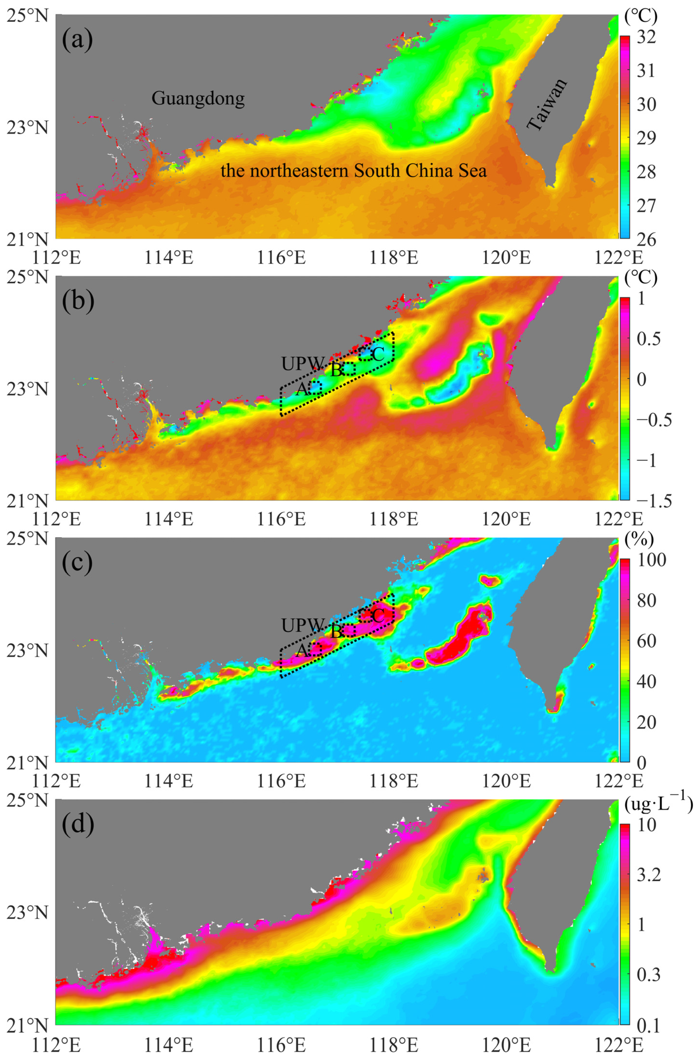
Figure 1.
Climatological (2003–2023) (a) sea surface temperature (SST), (b) topographic position index (TPI), (c) probability of TPI < −0.5, and (d) chlorophyll concentration (CHL) in the northeastern South China Sea (NESCS) during summer (June, July, and August); the boxes in (b,c) represent the regions of the coastal upwelling and its three cores focused upon in this study.
Previous studies have shown that the location of this coastal upwelling is mainly between 116 and 118°E [1,2]. This study calculates the topographical position index (TPI) by analyzing SST data and defines the boundary of the upwelling, which is marked as UPW by the parallelogram boxes in Figure 1b,c. In the UPW region, three upwelling cores can be further identified: UPW-A, UPW-B, and UPW-C. The calculation process of TPI is described in detail in Section 2.2.1 below, which means that the lower the TPI value, the stronger the upwelling [2,25]. According to the annual average of TPI in summer, we can see that the TPI in the UPW region is remarkably lower than that in other surrounding areas, and the TPIs in the UPW-A, UPW-B, and UPW-C regions are the three minimum cores of the UPW region. In addition, if we further analyze the probability of TPI less than −0.5, we can see that the probability of occurrence of low TPI in the UPW region is higher than that in the surrounding areas; in particular, the probabilities in the UPW-A, UPW-B, and UPW-C regions are the three peaks of the UPW region. It can be seen that these regions have a stable upwelling phenomenon, which can be used to characterize the coverage area of the upwelling and its central cores. Therefore, in the following analysis, we will use the statistical results of these regions to represent the upwelling intensity in their respective regions and then analyze the interannual variation in this upwelling.
2.2. Dataset
2.2.1. MODIS SST and CHL Data
This study utilized monthly mean SST and CHL data obtained from the MODIS onboard the Terra and Aqua satellites to analyze the interannual variations in coastal upwelling in the NESCS. MODIS, a medium-resolution imaging spectrometer carried on both Terra and Aqua satellites, is a crucial instrument in the Earth Observing System program of the United States for observing global biological and physical processes. Based on the thermal infrared radiation band, MODIS can acquire the thermal radiation flux of the Earth’s ocean surface and calculate sea surface temperature through atmospheric interactions [26]. The near-surface CHL is derived from remote sensing reflectances in the blue-to-green region of the visible spectrum using an empirical relationship.
The MODIS SST and CHL data can be applied to observe marine environmental changes, ecological factors, and ecosystem monitoring. The MODIS SST data analysis reveals essential information, such as ocean temperature gradients and ocean current distribution, holding significant value for marine science and resource management. Combined with calibration models and satellite assimilation data, it enables the estimation of the regions and seasons where upwelling occurs. The application of MODIS data in upwelling studies allows for assessing upwelling intensity and spatiotemporal distribution characteristics [27].
The data used in this study were obtained from the Oceancolor website of the National Aeronautics and Space Administration (http://oceandata.sci.gsfc.nasa.gov; accessed on 1 December 2023). The data have a spatial resolution of ~9 km, covering the entire northern South China Sea region, and a temporal resolution of monthly data spanning from 2003 to 2023.
2.2.2. ERA5 Wind Field Data
The relationship between upwelling and wind fields was analyzed using ERA5 wind field data. ERA5 is the fifth-generation atmospheric reanalysis dataset for global climate from January 1950, produced by the European Centre for Medium-Range Weather Forecasts (ECMWF). ERA5 is generated by the Copernicus Climate Change Service (C3S) of ECMWF. It contains atmospheric, land, and ocean climate variables hourly. ERA5 integrates model data with observational data from around the world, incorporating advanced numerical weather prediction models, ground observations, satellite data, and meteorological radar data to create a globally consistent dataset. The effectiveness of using ERA5 data to analyze wind speed in coastal upwelling regions has been validated [28,29]. Due to its global coverage and high spatiotemporal resolution, ERA5 finds applications in various fields, including wind energy data assessment, spatiotemporal analysis of precipitation data [30], and numerical simulations, such as Lagrangian transport simulations [31].
The ERA5 wind field data used in this study were downloaded from the Copernicus Climate Change Service website (https://cds.climate.copernicus.eu/#!/home; accessed on 1 December 2023). The data cover the entire South China Sea and parts of the western Pacific Ocean, with a spatial resolution of 0.25 degrees. The temporal span of the data matches that of SST, CHL, and other datasets used in this study.
2.2.3. Validity of the Data
In this paper, the MODIS monthly mean SST and CHL data were used to analyze the interannual variation in upwelling intensity, mainly considering the reliability of this dataset. We tried to apply the 8-day SST and CHL data by MODIS for analysis and found many missing values in the spatial coverage. Therefore, even if the 8-day data are adopted, it is still necessary to integrate the data into the monthly or seasonal mean data before further analysis. For this reason, this study directly adopts the monthly data products that are officially released. The data publisher has made finer revisions and more reasonable data integration, and the quality is guaranteed. In addition, since this paper focuses on the interannual change in upwelling, the focus is on the annual difference. Although this upwelling does have significant temporal changes within the season, it is not our focus.
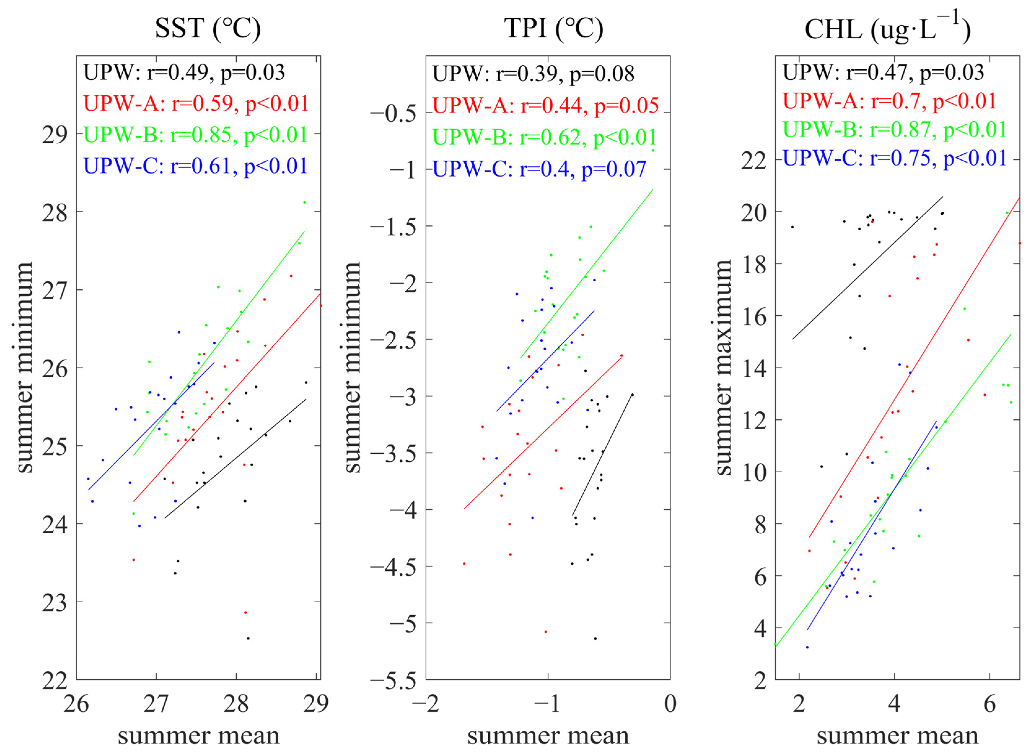
To verify the monthly data’s reliability, we specially analyzed the MODIS 8-day SST and CHL data from 2003 to 2023 and compared them with the monthly data. It can be found from Figure 2 that in the 21 years from 2003 to 2023, the summer mean SST/TPI/CHL obtained from the monthly data and the seasonal minimum SST/minimum TPI/maximum CHL obtained from the 8-day data are significantly correlated (p < 0.05 in most cases). It shows that the seasonal mean characteristics of the upwelling reflected in the monthly data are consistent with the seasonal high attributes reflected in the 8-day data. In addition, considering that MODIS data products have been widely used in many studies, the data quality has been fully verified [26,27]. Therefore, the MODIS monthly average data are feasible for synthesizing the seasonal data and then further analyzing the interannual variation in the upwelling.
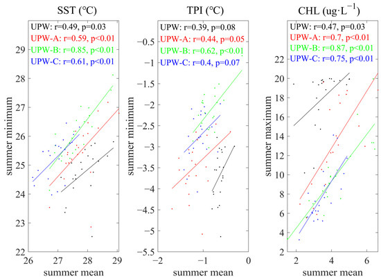
Figure 2.
Scatter comparisons of summer mean SST/TPI/CHL based on monthly MODIS data versus minimum SST/minimum TPI/maximum CHL based on 8-day MODIS data for the upwelling regions in the NESCS, as marked in Figure 1, during summers from 2003 to 2023.
2.3. Methodology
2.3.1. Topographic Position Index (TPI)
The TPI indicates the elevation difference between each unit within a region and the average elevation of the specified surrounding area. When applied to the upwelling scenario, the TPI can represent the difference in SST between the central unit and its surrounding region, reflecting upwelling intensity [2,25]. This application effectively removes the interannual signal of large-scale background temperatures. The formula for calculating the TPI is as follows:
where x and y represent the coordinates of the central point, N denotes the window size centered around the central point, and W(x, y) represents the average SST of all points within the scanning window. A negative TPI value indicates that the SST at the central point is lower than the surrounding environmental temperature. Therefore, in upwelling areas, the TPI is often negative. We utilized a square scanning window region with a side length of 150 km and a monthly average SST to calculate the TPI values.
2.3.2. Theil–Sen Estimation and Mann–Kendall Test
The Theil–Sen trend estimation method, or Sen’s slope estimator, is a robust non-parametric statistical approach for trend estimation [32,33]. This method is computationally efficient and insensitive to measurement errors and outliers, making it suitable for the trend analysis of long-time series data. For a time series xi (i = 1, 2, 3, …, n) consisting of n independent and identically distributed samples of random variables, the calculation formula for estimating the trend is as follows:
where β is the trend or the Sen slope, and xj and xi denote the series values at j and i, respectively. The sign of β indicates the direction of the trend change: if greater (less) than zero, it signifies a positive (negative) change.
Additionally, the non-parametric statistical Mann–Kendall trend test was applied to estimate the significance of the trend in the series. The basic idea is to examine the trend in the sequence by comparing the size relationships between each pair of data points and then determine the direction of the trend based on the sign of the sum of ranks [34,35]. The statistic S for the test is calculated by
The test statistic S follows a normal distribution. When n > 10, the normal distribution statistic Z can be calculated as follows:
where Var(S) represents the variance of:
In the two-sided test, at a given significance level α, if |Z| ≥ Z1−α/2, the null hypothesis is rejected, indicating a significant upward (Z > 0) or downward trend (Z < 0) in the series data, with the magnitude of Z determining the significance of the trend. This study set a 95% threshold confidence level (α = 0.05) for the test.
The Theil–Sen and the Mann–Kendall analyses are widely applied in ocean science for trend estimations, predictions, and significance assessments. For instance, they were used to analyze variations in meteorological variables [36], examine trend differences in fitting non-stationary extreme wave height models with different climate change datasets [33], and assess the long-term characteristics of wave energy resources in China’s coastal areas [35].
3. Results
3.1. Interannual Variations in Coastal Upwelling
Based on MODIS data, the spatial distribution of annual summer average SST, TPI, and CHL in the NESCS was obtained (Figure 1). As shown in the figure, a coastal upwelling area is characterized by low SST, low TPI, and high CHL off the eastern coast of Guangdong. The TPI shows that the coastal upwelling mainly covers the sea area between 116°E and 118°E and approximately 0.5° latitudes offshore, marked as the UPW area in Figure 1b. In this upwelling region of UPW, three core regions, UPW-A, UPW-B, and UPW-C, with a range of 0.2° × 0.2°, can be further indicated based on their relatively low TPI values.
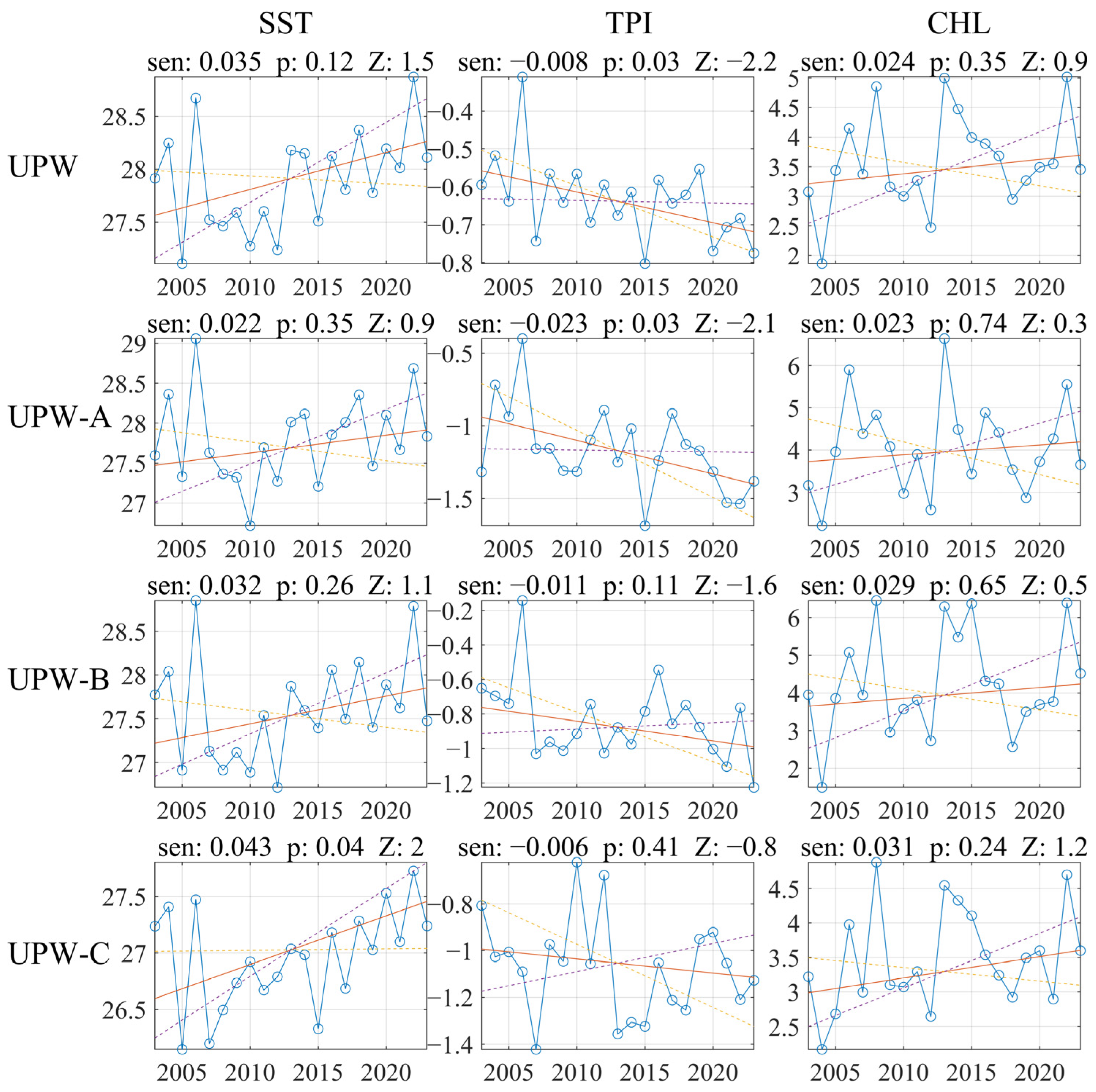
Figure 3 illustrates the average SST, TPI, and CHL of the UPW, UPW-A, UPW-B, and UPW-C regions during the summer yearly. The results show that there are interannual variations and clear long-term trends in all the three variables. Conducting Theil–Sen estimation and the Mann–Kendall test on these interannual variation data, it was found that the SST and upwelling intensity in the regions have shown a significant upward trend in the past 21 years. Although CHL shows an upward trend, the trend is not significant. The trends in the three core regions are different. As we move northward, the warming trend of SST becomes more substantial, the strengthening trend of upwelling becomes weaker, and the increasing trend of CHL becomes higher.
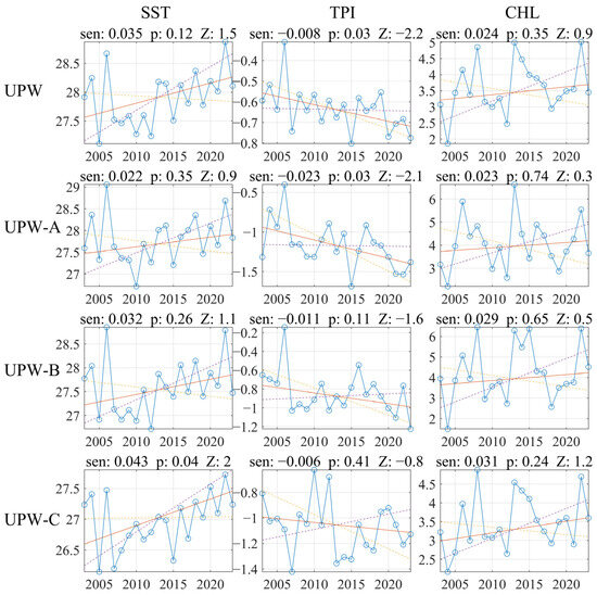
Figure 3.
Annual variation in summer mean SST (°C), TPI (°C), and CHL (mg/m3) in the upwelling regions of the NESCS, as marked in Figure 1. The dots with lines represent the SST/TPI/CHL, the solid lines represent the trend by Theil–Sen estimation, and the dashed lines represent the confidence intervals.
The spatial distribution of the Sen slope of SST, TPI, and CHL can provide a clearer understanding of the regional characteristics of long-term trends (Figure 4). From the SST trend, the entire NESCS exhibits a significant warming trend, especially in the open sea areas far from the coastal upwelling regions, which may be related to global warming caused by climate change [37]. The TPI generally shows a decreasing trend in coastal areas, indicating that the intensity of upwelling along the coast has significantly increased in the recent 20 years, especially in the core regions such as UPW-A, UPW-B, and UPW-C, where the decreasing trend of TPI values is significant (p < 0.05) (Figure 4b).
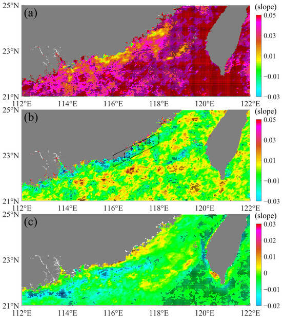
Figure 4.
Spatial distribution of the Sen slopes of the summer seasonal mean (a) SST (°C/year), (b) TPI (°C/year), and (c) CHL (mg/m3/year) in the NESCS during 2003–2023. Trends values that are statistically significant (p < 0.05) according to the Mann–Kendall test are marked as black crosses.
It is worth noting that the long-term trend of CHL in the nearshore area is opposite to that in the open sea due to the influence of upwelling. In the open sea area, the summer SST is generally high, and the increase in SST further inhibits chlorophyll growth. However, in the coastal upwelling region, the nutrient-rich cold water brought by upwelling from the slope and shelf towards the shore promotes the growth of CHL, creating a long-term increasing trend. Upwelling may also combine with the transport of coastal currents, resulting in a more robust increase of CHL in the northeast compared to the southwest (i.e., UPW-C > UPW-B > UPW-A, in Figure 3). The results indicate that in climate warming, upwelling plays a crucial role in maintaining the health of the nearshore ecosystem.
3.2. Relationship between Wind Field and Upwelling
Previous studies have shown that wind field variation can lead to CHL increase through various dynamic mechanisms in the SCS [13,14]. The ERA5 wind data reveal that the nearshore NESCS exhibits significant southwest winds in summer (Figure 5). As shown in the figure, a prominent high (low) value area of the alongshore (onshore) wind component covers the coastal upwelling region. The southwest monsoon is the primary mechanism that generates coastal upwelling in the northern regions of the SCS [1,7,9,11]. When the southwest monsoon intensifies, wind-induced Ekman transport in the offshore direction increases, and the seawater near the northeast coast of the SCS flows in the offshore direction. Then, the water level near the shore decreases. The cold water near the shore forms a pressure gradient force due to the offshore formation of the upper layer of seawater, supplementing the upper layer of seawater and forming an upward onshore flow.
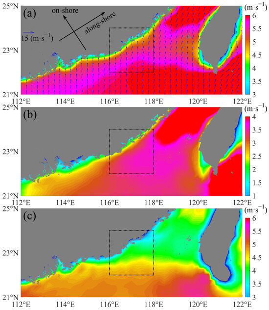
Figure 5.
Climatological (2003–2023) (a) sea surface wind field and its (b) alongshore and (c) onshore components in the NESCS during summer. The box denotes the statistical region of Figure 6.
Further data analysis reveals that the sea surface winds in the coastal NESCS exhibit significant interannual variation characteristics (Figure 6). As shown in the figure, although the variation in wind speed is not apparent, there is a remarkable interannual decrease in the onshore component. This has led to significant clockwise changes in the direction of the wind, which is conducive to the alongshore component generating coastal upwelling. The change magnitude exceeds half of its annual average. Considering the critical role of Ekman transport in this nearshore upwelling [1,7,9,11], interannual variations in the wind field may be the main factor affecting the long-term trend and interannual variation in the upwelling intensity along the coast of the NESCS.
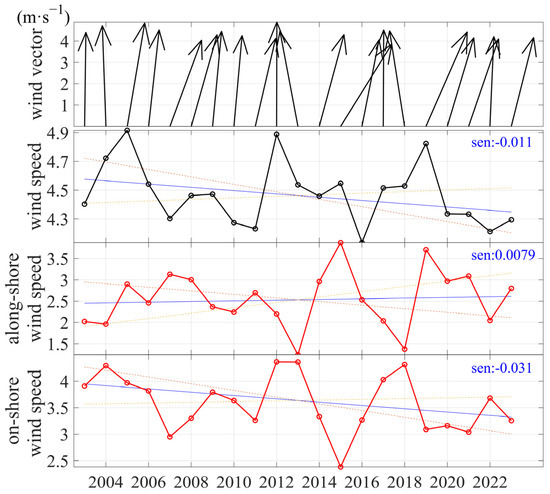
Figure 6.
Multiyear series of the average wind vector and the total, alongshore, and onshore wind speeds in the NESCS during summers. The statistical region is the box in Figure 5. The dots with lines represent the total/alongshore/onshore wind speeds, the solid lines represent the trend by Theil–Sen estimation, and the dashed lines represent the confidence intervals.
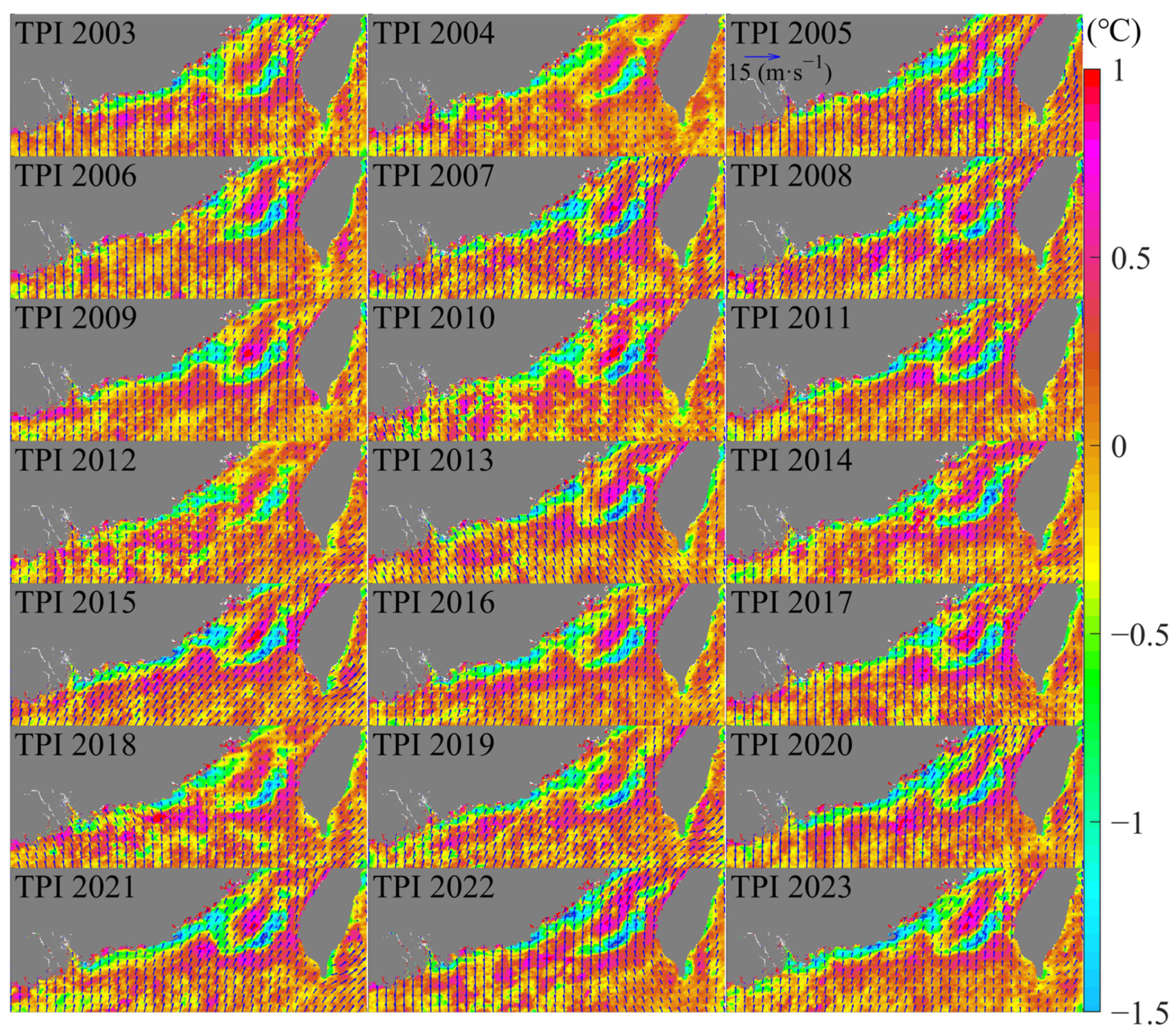
The yearly spatial distribution of TPI and sea surface wind field for summers from 2002 to 2023 show good agreement between the intensity of upwelling and the direction of sea surface wind (Figure 7). For example, during the summer of 2006, the wind direction significantly tended northwards, and the intensity of the nearshore upwelling was considerably weaker, with its affecting area being relatively small that year. By contrast, in the summer of 2007, the wind direction significantly tended towards the east. The intensity of the nearshore upwelling was considerably stronger than in the summer of 2006, with a significantly larger affecting area.
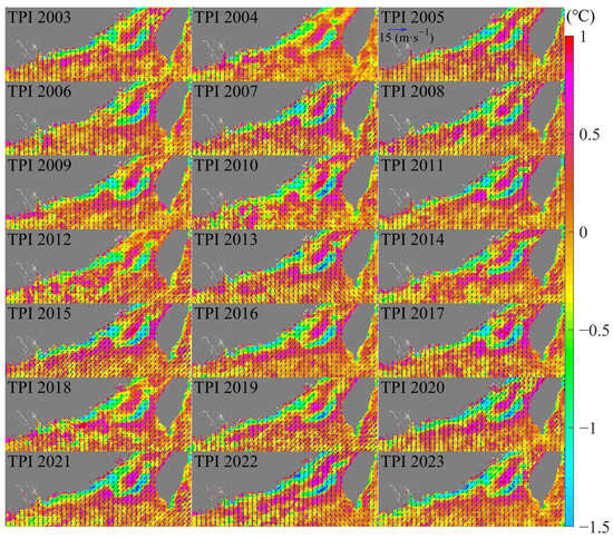
Figure 7.
Spatial distributions of the summer seasonal mean topographic position index (TPI) and wind field in the NESCS from 2002 to 2023.
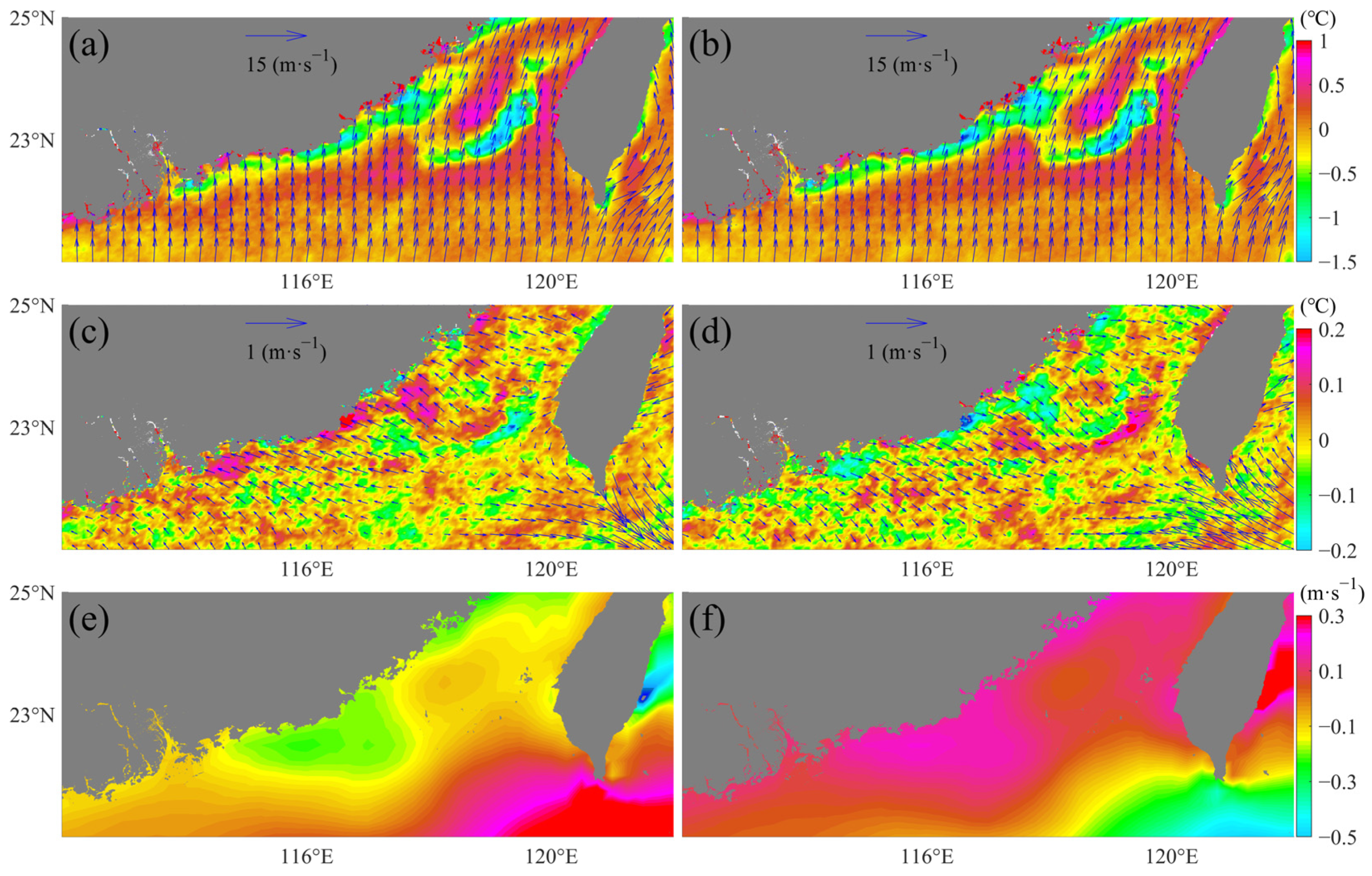
To further clarify the matching pattern between the upwelling intensity and wind fields, the 21-year data were divided into two groups with strong and weak upwelling intensity, based on the Theil–Sen trend analysis results of TPI (Figure 3): the years in the UPW area in which the TPI values are below (above) the trend line are regarded as years with strong (weak) upwelling intensity. Then, a composite analysis of the sea surface wind field and TPI was conducted based on the two groups of data, respectively (Figure 8). The composite analysis results show that in years with lower TPI values (right panels of Figure 8), the wind direction shows a southeast anomaly compared to the climatology; that is, the wind tends to blow along the coast or towards the offshore direction, with the alongshore wind component substantially increasing in the eastern Guangdong coastal area. Such a wind field is more conducive to the generation of coastal upwelling. In contrast, in the years with high TPI values (left panels of Figure 8), the wind tends to blow northward or onshore, which is not conducive to the formation of upwelling. Previous studies have pointed out that abnormal changes in wind fields, especially wind direction, are critical factors in enhancing nearshore upwelling [7,24]. The results of this study further propose the matching relationship between the intensity of coastal upwelling in the NESCS and the interannual variation in the wind field through composite analysis.
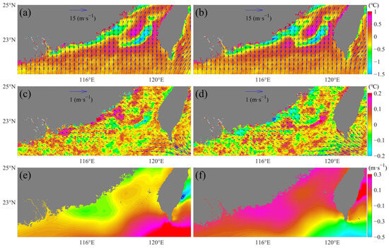
Figure 8.
The summer-seasonal composite wind fields and TPI values in the NESCS during (a) weak and (b) strong upwelling years, as well as (c,d) their anomalies relative to the climatological means, and (e,f) the alongshore components of the wind anomalies. The weak (strong) upwelling years are when the summer TPI values in the UPW region are above (below) the trend line in Figure 3.
3.3. Predictability of Upwelling Combined with ENSO
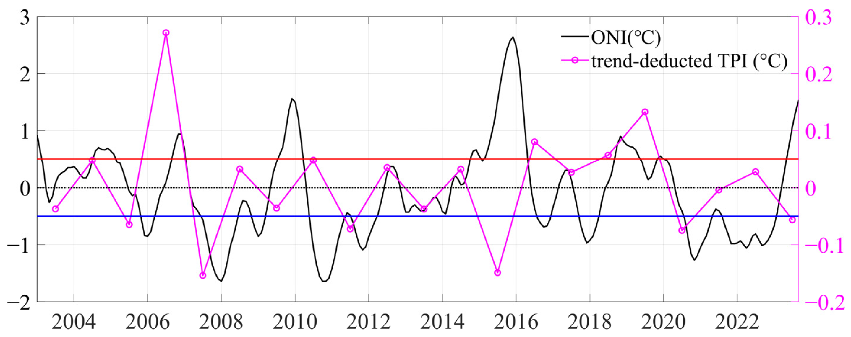
The previous paragraph revealed that the interannual variations in the coastal upwelling in the NESCS are closely related to the interannual variations in the wind field. Considering that the monsoons in the SCS are controlled by large-scale Western Pacific wind fields [7,17], it is necessary to analyze the relationship between upwelling and climate factors such as ENSO. Analysis of the Ocean Niño Index (ONI) and the TPI deducted from the interannual trend indicates a good correlation between them (Figure 9). In the years with more vigorous upwelling (lower TPI) in summer, such as 2003, 2005, 2007, 2015, 2020, and 2023, the ONI during the previous winter generally appears to be El Niño events.
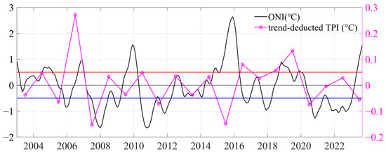
Figure 9.
The series of the Oceanic Niño Index (ONI) and the summer TPI in the UPW region after deducting its long-term trend. The blue, red, and dashed lines indicate that the ONI value equals to 0.5, –0.5, and 0, respectively.
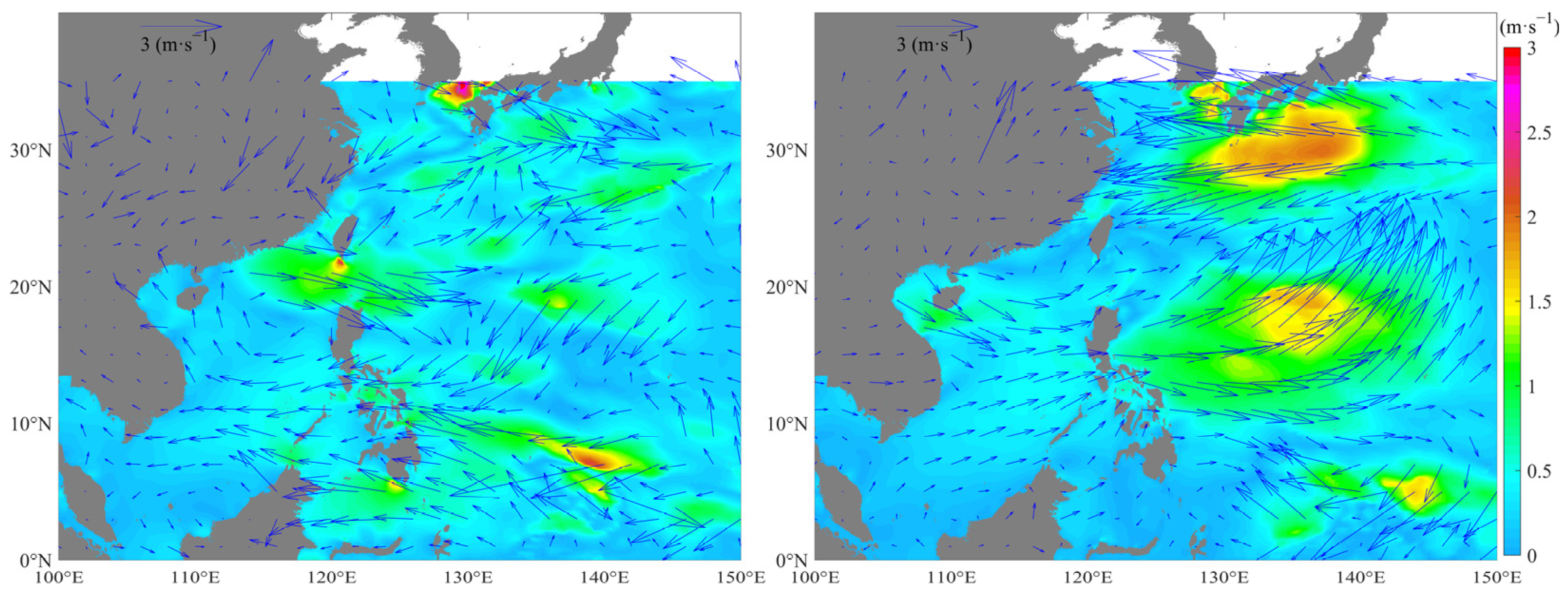
Previous studies have shown that the El Niño phenomenon can affect the strength of coastal upwelling in the SCS by altering the wind speed and direction of the monsoon. Accompanied by the El Niño phenomenon, an anticyclonic (i.e., clockwise) circulation anomaly centered on the NESCS [17,19,20]. This impact will significantly affect the SCS wind field, causing changes in the monsoon [18] and thereby causing differentiated effects on upwelling. Such a mechanism can be further confirmed through a composite analysis of the summer wind field following El Niño and La Niña events from 2002 to 2023 (Figure 10). In the summer following El Niño, the anomalous anticyclone wind field centered on the NESCS caused the sea surface wind near the Guangdong Province coast to deflect towards the southeast. The wind blowing northeast (alongshore) was strengthened. This type of wind will enhance offshore Ekman transport, thereby increasing the upward climb of bottom seawater for replenishment. In contrast, a cyclonic (counter-clockwise) anomaly in the wind field strengthened during the summers of the following year of La Niña. The wind field around the Guangdong coast shifted northwestward, which was not conducive to forming the coastal upwelling.

Figure 10.
Composite wind field anomalies in the South China Sea and Western Pacific during the summer following the (left panel) El Niño and (right panel) La Niña years.
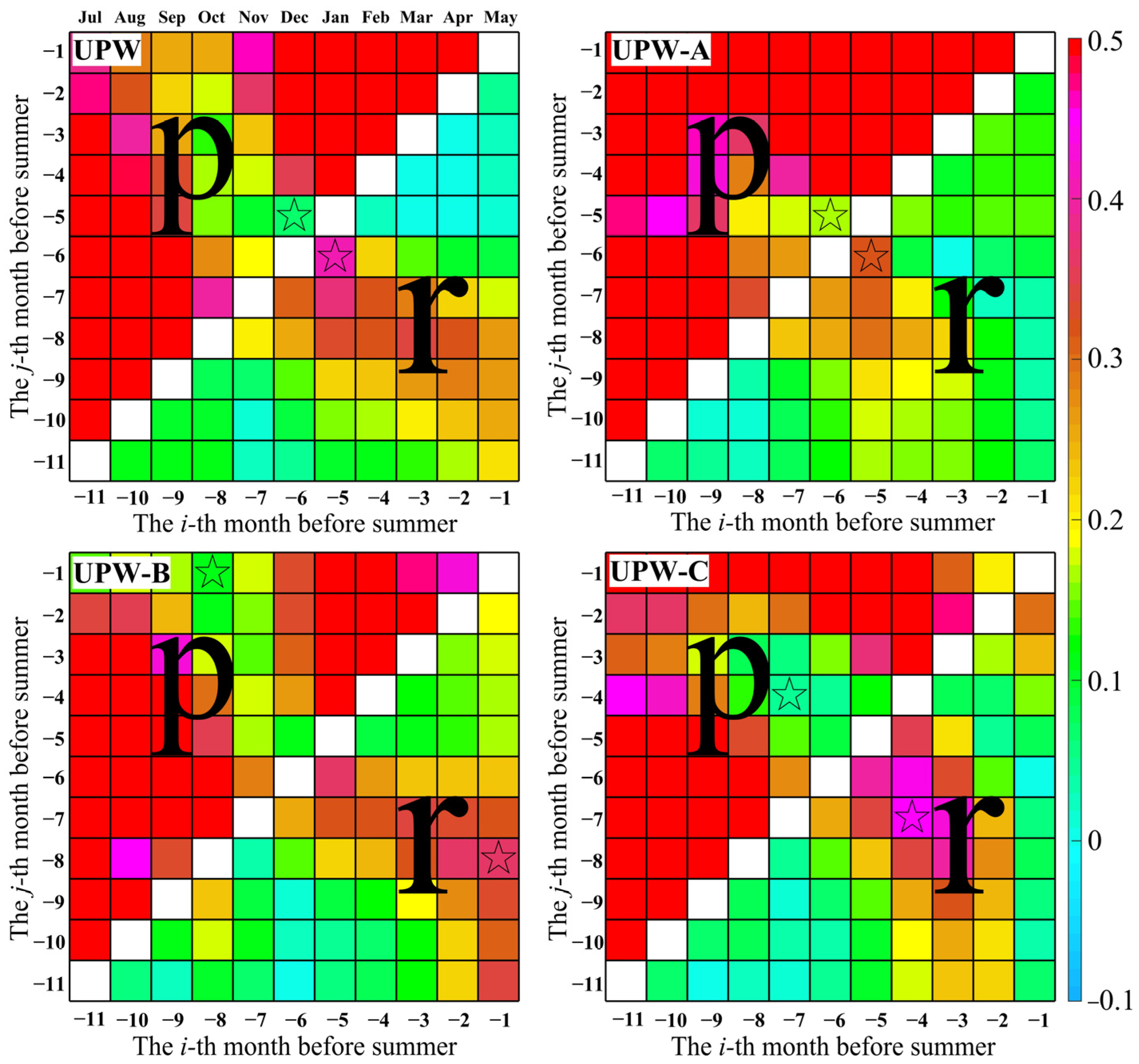
The relationship between upwelling intensity and ENSO can be used to predict the intensity of upwelling. First, subtract the ONI corresponding to the i-th and j-th months before given summers, and perform correlation analysis between the different i and j combinations and TPI. The results can help find the optimal correlation between the change rate of the ONI and the TPI (Figure 11). The results show a significant correlation between the intensity of summer upwelling and the previous winter ONI changes. For example, for the entire upwelling zone (UPW), there is the most significant correlation between TPI values and the difference in ONI between December of the previous year and January of the current year (r = 0.42, p = 0.07). This indicates that the higher the increase (decrease) in ONI from December to January, the greater the negative (positive) value of TPI in the following summer, resulting in a higher (lower) intensity of upwelling.
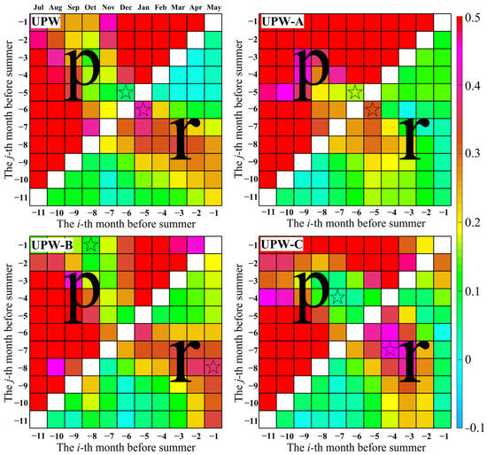
Figure 11.
The correlation coefficient r between the TPI and the ONI change rate (i.e., ONIi–ONIj). The corresponding p-value is displayed after transposition on the top-left corner of each panel for the upwelling regions (i.e., UPW, UPW-A, UPW-B, and UPW-C marked in Figure 1). The −11th to −6th months represent July to December of the previous years, and the −5th to −1st months represent January to May before the given summer. The stars denote the most significant correlations with the lowest p-value and its corresponding r-value for the upwelling regions.
The above correlation analysis indicates that the changes in ONI have important predictive significance for the intensity of upwelling in the following summer. Based on this, an attempt is made to construct a prediction of upwelling intensity based on the ONI, which can further fit the following empirical formula:
where β is the long-term trend (Sen slope), which is estimated above in Section 3.1, and i and j are the months with the highest correlation between ONI change rate (ONIi–ONIj) and TPI (Figure 11). For example, for the UPW region, i = −5, j = −6. The parameters k and b can be linearly fitted by substituting the TPI and ONI values.
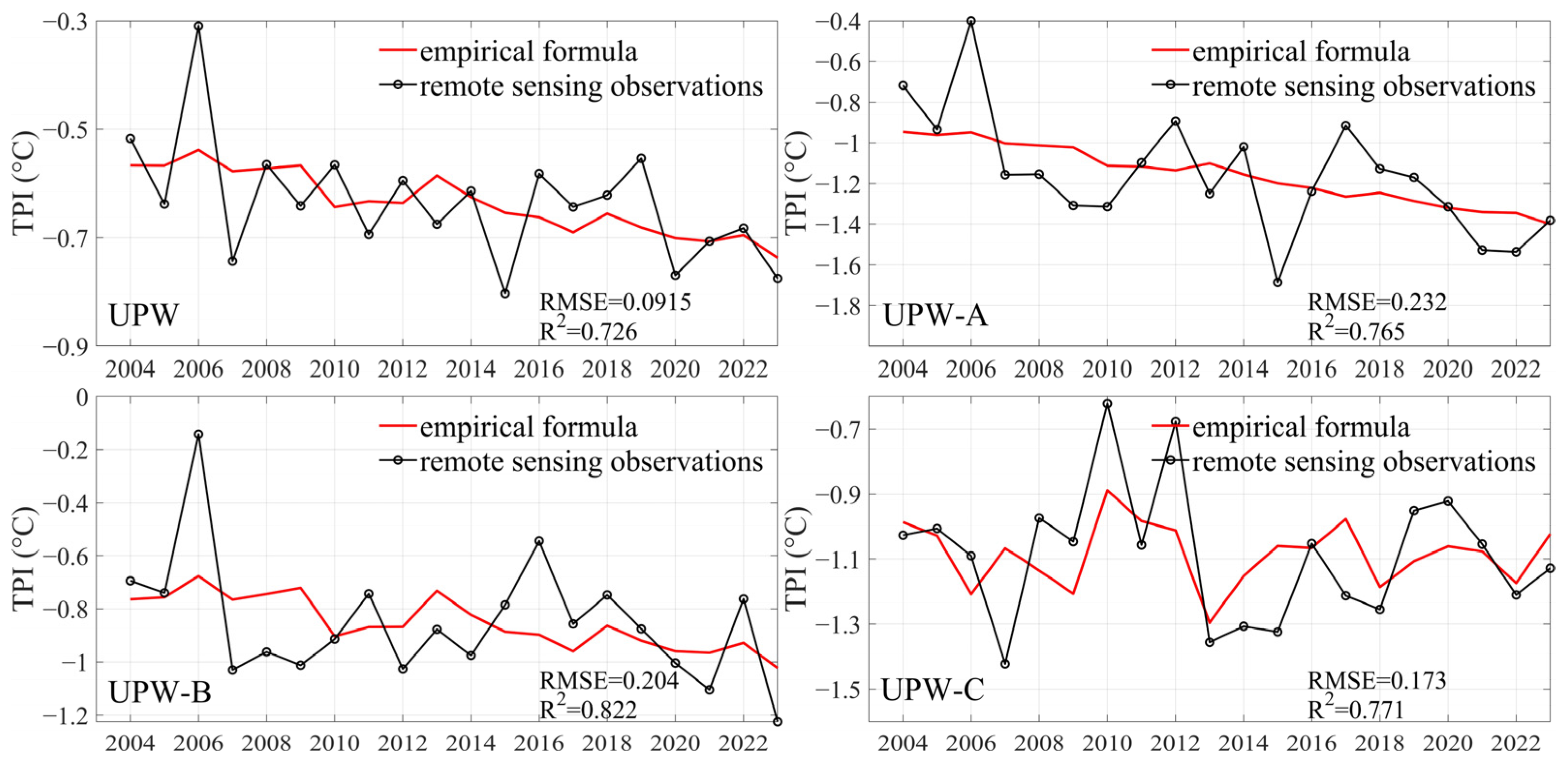
The comparison between the predicted results of the fitted empirical formula and the measured values based on satellite observations is shown in Figure 12. The results show that the empirical formula can well reproduce most of the variations in TPI, and the determination coefficient R2 is between 0.72 and 0.82. However, probably because other climate factors, rather than ENSO, also constrain the wind field and upwelling, the prediction performance is still not ideal, especially for the years in which TPI values were significantly higher or lower than the average level. Therefore, to achieve a more accurate prediction of the TPI, more factors may need to be further considered.
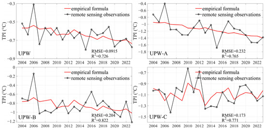
Figure 12.
Comparison of the TPI series between the empirical formula (Equation (7)) and remote sensing observations for the upwelling regions (i.e., UPW, UPW-A, UPW-B, and UPW-C marked in Figure 1).
4. Discussion
Many studies have shown that CHL in the SCS has significant annual periodic variation characteristics, e.g., [13,14]. In relatively deep areas, the driving factors of this periodic variation are mainly related to the deepening of the mixing layer caused by the strengthening of the wind field and the pumping caused by the eddies [13,14,15]. For coastal waters, such as eastern Guangdong, eastern Hainan Island, and east Vietnam, the high CHL in summer is mainly related to the coastal upwelling caused by Ekman transport. The primary mechanism is that the wind blowing to the northeast along the coastline in summer causes offshore Ekman transport of the surface water, resulting in the upwelling of the lower nutrient-rich water onshore across the continental shelf [7,12,23]. The results of this study also show that the coastal waters of eastern Guangdong have the characteristics of low SST and high CHL upwelling in summers. Their occurrence is closely related to the enhancement of the wind field (Figure 8). Based on previous studies, the results of this paper further analyze the interannual variation characteristics of this upwelling. Our research reveals that the interannual variation in large-scale climate factors can significantly impact the wind field of the SCS (Figure 10), which will cause variations in the upwelling in the NESCS. These findings can provide essential support for the accurate prediction of coastal upwelling.
In addition to the SCS, there are many marginal sea areas worldwide, such as the Arabian Sea and the Baltic Sea, which have significant coastal upwelling phenomena, mainly driven by Ekman transport [12]. However, in the background of global climate change, the intensities of coastal upwellings in these regions appear to be different long-term trends. Even in the same sea, the variation trends of upwelling at various coastal locations can be significantly different [12]. Taking the SCS as an example, other authors’ study results also found that coastal upwelling in the NESCS showed a significant intensifying trend [22], which is consistent with the results of this paper. However, in the Taiwan Strait, which is not far from our study region, the interannual variation in upwelling shows a significant weakening trend [21]. The difference in trends between the two areas may be related to the spatial difference in wind field changes. For example, a clockwise abnormal wind in Taiwan Straight might be onshore in the left coastal region but offshore in the right coastal region (Figure 8 and Figure 10), favorable for the coastal upwelling in eastern Guangdong, but unfavorable for the upwelling in the west of Taiwan. In addition, for sea areas such as east Hainan in the SCS, Arabian Sea, and Baltic Sea, the interannual variation characteristics of coastal upwelling are also very complicated [12]. Therefore, to accurately predict the long-term trends of these coastal upwellings, it is necessary to accurately predict the long-term wind field by constructing a sufficiently comprehensive climate model.
Although the long-term trend of coastal upwelling in the NESCS and its influencing factors are clarified in this paper, more data and works, including field observations and numerical simulations, may be needed to assess the quantitative measurement of the upwelling intensity. Ocean color satellite data can be susceptible to various factors, such as cloud cover and rain, affecting their quality and accuracy. It is essential to adopt appropriate algorithms to convert the signals obtained from remote sensing into directly applicable data, which is also revealed in studies regarding, for example, CHL mapping with Sentinel 2 or 3 and bathymetry mapping with satellite images [38,39]. For different types of coastal waters characterized by bathymetry and distance to the coast, corresponding suitable algorithms are needed [38,40]. Because this paper focuses on the long-term trend, even if there is an inaccuracy in the data, it is only the systematic error of the region, which does not affect the accurate judgment of the long-term trend. However, suppose it is necessary to measure the specific value of the upwelling intensity or CHL variations; in that case, it may be necessary to thoroughly verify the algorithm of inversion processes with more in situ data.
5. Conclusions
This study used MODIS satellite remote sensing data, such as sea surface temperature (SST) and chlorophyll (CHL), combined with ERA5 reanalysis wind field data, to systematically study the interannual variation patterns of summer coastal upwelling off the eastern part of Guangdong Province in the Northeastern South China Sea (NESCS). On this basis, the relationship between the intensity of the upwelling and abnormal changes in wind fields was analyzed, and the feasibility of predicting the intensity of upwelling based on climate factors, such as the Ocean Niño Index (ONI), was discussed.
The main conclusions indicate that the summer coastal upwelling intensity and SST in the NESCS areas significantly increased between 2003 and 2023. Affected by rising SST and enhanced upwelling, the CHL appears to have an increased trend, although it has not reached a significant level.
Moreover, the interannual variation in and long-term trend of the upwelling intensity are closely related to sea surface wind fields. In the years when the wind field appears as a clockwise anomaly centered on the NESCS, the wind direction tends to parallel to the shoreline, and the upwelling strengthens. In contrast, in the years when the wind direction deviates from the clockwise anomaly and tends to be onshore, the upwelling is relatively weak. The agreement between large-scale climate indices (e.g., the ONI) and the wind field can help achieve preliminary predictions of the trend and interannual characteristics of the upwelling intensity. In the future, for more accurate assessments and forecasts of the upwelling intensity and the relative CHL variations, it may be necessary to employ more in situ data to validate the remote sensing products and include more complex climatical or local factors into the prediction model.
Author Contributions
Conceptualization, J.L.; methodology, W.C.; software, W.C.; validation, J.L.; formal analysis, W.C. and Y.T.; investigation, W.C. and W.L.; resources, J.L. and P.S.; data curation, W.C.; writing—original draft preparation, W.C., Y.T. and J.L.; writing—review and editing, J.L. and W.W.; visualization, W.C.; supervision, J.L. and W.W.; project administration, J.L.; funding acquisition, J.L. and Y.D. All authors have read and agreed to the published version of the manuscript.
Funding
This study was funded by the Science and Technology Projects of Guangdong Province (2021B1212050023), the Guangdong Basic and Applied Basic Research Foundation (2023A1515011497), the foundation of Guangdong Provincial Observation and Research Station for Coastal Upwelling Ecosystem (CUE202301), the Hainan Provincial Natural Science Foundation of China (422MS160), and the development fund of the South China Sea Institute of Oceanology of the Chinese Academy of Sciences (SCSIO202207).
Data Availability Statement
The MODIS data are available on the Oceancolor website of the National Aeronautics and Space Administration (http://oceandata.sci.gsfc.nasa.gov, accessed on 1 December 2023). The ERA5 data are available on the Copernicus Climate Data Store website (http://climate.copernicus.eu/climate-reanalysis/, accessed on 1 December 2023).
Acknowledgments
The analysis in this study was supported by the High-Performance Computing Division at the South China Sea Institute of Oceanology.
Conflicts of Interest
The authors declare no conflicts of interest.
References
- Hu, J.; Wang, X.H. Progress on upwelling studies in the China seas. Rev. Geophys. 2016, 54, 653–673. [Google Scholar] [CrossRef]
- Shi, W.; Huang, Z.; Hu, J. Using TPI to map spatial and temporal variations of significant coastal upwelling in the northern South China Sea. Remote Sens. 2021, 13, 1065. [Google Scholar] [CrossRef]
- Hsiao, P.-Y.; Shimada, T.; Lan, K.-W.; Lee, M.-A.; Liao, C.-H. Assessing summer time primary production required in changed marine environments in upwelling ecosystems around the Taiwan bank. Remote Sens. 2021, 13, 765. [Google Scholar] [CrossRef]
- Li, D.; Yang, S.; Wei, Y.; Wang, X.; Mao, Y.; Guo, C.; Sun, J. Response of size-fractionated chlorophyll a to upwelling and Kuroshio in northeastern South China Sea. J. Mar. Sci. Eng. 2022, 10, 784. [Google Scholar] [CrossRef]
- Gan, J.; Cheung, A.; Guo, X.; Li, L. Intensified upwelling over a widened shelf in the northeastern South China Sea. J. Geophys. Res. Oceans 2009, 114, C09019. [Google Scholar] [CrossRef]
- Gan, J.; Li, L.; Wang, D.; Guo, X. Interaction of a river plume with coastal upwelling in the northeastern South China Sea. Cont. Shelf Res. 2009, 29, 728–740. [Google Scholar] [CrossRef]
- Jing, Z.; Qi, Y.; Du, Y. Upwelling in the continental shelf of northern South China Sea associated with 1997–1998 El Niño. J. Geophys. Res. Oceans 2011, 116, C02033. [Google Scholar] [CrossRef]
- Shu, Y.; Wang, D.; Zhu, J.; Peng, S. The 4-D structure of upwelling and Pearl River plume in the northern South China Sea during summer 2008 revealed by a data assimilation model. Ocean Model. 2011, 36, 228–241. [Google Scholar] [CrossRef]
- Gu, Y.; Pan, J.; Lin, H. Remote sensing observation and numerical modeling of an upwelling jet in Guangdong coastal water. J. Geophys. Res. Oceans 2012, 117, C08019. [Google Scholar] [CrossRef]
- Wang, D.; Zhuang, W.; Xie, S.-P.; Hu, J.; Shu, Y.; Wu, R. Coastal upwelling in summer 2000 in the northeastern South China Sea. J. Geophys. Res. Oceans 2012, 117, C04009. [Google Scholar] [CrossRef]
- Wang, D.; Shu, Y.; Xue, H.; Hu, J.; Chen, J.; Zhuang, W.; Zu, T.; Xu, J. Relative contributions of local wind and topography to the coastal upwelling intensity in the northern South China Sea. J. Geophys. Res. Oceans 2014, 119, 2550–2567. [Google Scholar] [CrossRef]
- Satar, M.N.; Akhir, M.F.; Zainol, Z.; Chung, J.X. Upwelling in marginal seas and its association with climate change scenario—A comparative review. Climate 2023, 11, 151. [Google Scholar] [CrossRef]
- Liu, F.; Chen, C.; Zhan, H. Decadal variability of chlorophyll a in the South China Sea: A possible mechanism. Chin. J. Oceanol. Limnol. 2012, 30, 1054–1062. [Google Scholar] [CrossRef]
- Xian, T.; Sun, L.; Yang, Y.-J.; Fu, Y.-F. Monsoon and eddy forcing of chlorophyll-a variation in the northeast South China Sea. Int. J. Remote Sens. 2012, 33, 7431–7443. [Google Scholar] [CrossRef]
- Li, J.; Qi, Y.; Jing, Z.; Wang, J. Enhancement of eddy-Ekman pumping inside anticyclonic eddies with wind-parallel extension: Satellite observations and numerical studies in the South China Sea. J. Marine Syst. 2014, 132, 150–161. [Google Scholar] [CrossRef]
- Vaidya, H.N.; Breininger, R.D.; Madrid, M.; Lazarus, S.; Kachouie, N.N. Generalized additive models for predicting sea level rise in coastal Florida. Geosciences 2023, 13, 310. [Google Scholar] [CrossRef]
- Li, S.; Li, Y.; Peng, S.; Qi, Z. The inter-annual variations of the significant wave height in the Western North Pacific and South China Sea region. Clim. Dynam. 2021, 56, 3065–3080. [Google Scholar] [CrossRef]
- Hong, B.; Zhang, J. Long-term trends of sea surface wind in the northern South China Sea under the background of climate change. J. Mar. Sci. Eng. 2021, 9, 752. [Google Scholar] [CrossRef]
- Xie, S.-P.; Kosaka, Y.; Du, Y.; Hu, K.; Chowdary, J.S.; Huang, G. Indo-Western Pacific Ocean capacitor and coherent climate anomalies in post-ENSO summer: A review. Adv. Atmos. Sci. 2016, 33, 411–432. [Google Scholar] [CrossRef]
- Wang, B.; Huang, F.; Wu, Z.; Yang, J.; Fu, X.; Kikuchi, K. Multi-scale climate variability of the South China Sea monsoon: A review. Dynam. Atmos. Oceans 2009, 47, 15–37. [Google Scholar] [CrossRef]
- Praveen, V.; Ajayamohan, R.S.; Valsala, V.; Sandeep, S. Intensification of upwelling along Oman coast in a warming scenario. Geophys. Res. Lett. 2016, 43, 7581–7589. [Google Scholar] [CrossRef]
- Liu, S.; Zuo, J.; Shu, Y.; Ji, Q.; Cai, Y.; Yao, J. The intensified trend of coastal upwelling in the South China Sea during 1982–2020. Front. Mar. Sci. 2023, 10, 1084189. [Google Scholar] [CrossRef]
- Tang, D.; Kawamura, H.; Dien, T.V.; Lee, M. Offshore phytoplankton biomass increase and its oceanographic causes in the South China Sea. Mar. Ecol. Prog. Ser. 2004, 268, 31–41. [Google Scholar] [CrossRef]
- Zhang, C. Responses of summer upwelling to recent climate changes in the Taiwan Strait. Remote Sens. 2021, 13, 1386. [Google Scholar] [CrossRef]
- Ware, D.M.; Thomson, R.E. Link between long-term variability in upwelling and fish production in the northeast Pacific Ocean. Can. J. Fish. Aquat. Sci. 1991, 48, 2296–2306. [Google Scholar] [CrossRef]
- Walton, C.C.; Pichel, W.G.; Sapper, J.F.; May, D.A. The development and operational application of nonlinear algorithms for the measurement of sea surface temperatures with the NOAA polar-orbiting environmental satellites. J. Geophys. Res. Oceans 1998, 103, 27999–28012. [Google Scholar] [CrossRef]
- Dabuleviciene, T.; Kozlov, I.E.; Vaiciute, D.; Dailidiene, I. Remote sensing of coastal upwelling in the south-eastern Baltic Sea: Statistical properties and implications for the coastal environment. Remote Sens. 2018, 10, 1752. [Google Scholar] [CrossRef]
- Strub, P.T.; James, C. Evaluation of nearshore QuikSCAT 4.1 and ERA-5 wind stress and wind stress curl fields over eastern boundary currents. Remote Sens. 2022, 14, 2251. [Google Scholar] [CrossRef]
- Ferreira, S.; Sousa, M.; Picado, A.; Vaz, N.; Dias, J.M. New insights about upwelling trends off the Portuguese coast: An ERA5 dataset analysis. J. Mar. Sci. Eng. 2022, 10, 1849. [Google Scholar] [CrossRef]
- Jiao, D.; Xu, N.; Yang, F.; Xu, K. Evaluation of spatial-temporal variation performance of ERA5 precipitation data in China. Sci. Rep. 2021, 11, 17956. [Google Scholar] [CrossRef] [PubMed]
- Hoffmann, L.; Guenther, G.; Li, D.; Stein, O.; Wu, X.; Griessbach, S.; Heng, Y.; Konopka, P.; Mueller, R.; Vogel, B.; et al. From ERA-Interim to ERA5: The considerable impact of ECMWF’s next-generation reanalysis on Lagrangian transport simulations. Atmos. Chem. Phys. 2019, 19, 3097–3124. [Google Scholar] [CrossRef]
- De Leo, F.; Besio, G.; Briganti, R.; Vanem, E. Non-stationary extreme value analysis of sea states based on linear trends. Analysis of annual maxima series of significant wave height and peak period in the Mediterranean Sea. Coast. Eng. 2021, 167, 103896. [Google Scholar] [CrossRef]
- Vanem, E. Non-stationary extreme value models to account for trends and shifts in the extreme wave climate due to climate change. Appl. Ocean Res. 2015, 52, 201–211. [Google Scholar] [CrossRef]
- Zhao, P.; He, Z. Temperature Change Characteristics in Gansu Province of China. Atmosphere 2022, 13, 728. [Google Scholar] [CrossRef]
- Sun, P.; Xu, B.; Wang, J. Long-term trend analysis and wave energy assessment based on ERA5 wave reanalysis along the Chinese coastline. Appl. Energy 2022, 324, 119709. [Google Scholar] [CrossRef]
- Gocic, M.; Trajkovic, S. Analysis of changes in meteorological variables using Mann-Kendall and Sen’s slope estimator statistical tests in Serbia. Global Planet. Change 2013, 100, 172–182. [Google Scholar] [CrossRef]
- Zhang, Y.; Du, Y.; Feng, M.; Hobday, A.J. Vertical structures of marine heatwaves. Nat. Commun. 2023, 14, 6483. [Google Scholar] [CrossRef] [PubMed]
- Tran, M.D.; Vantrepotte, V.; Loisel, H.; Oliveira, E.N.; Tran, K.T.; Jorge, D.; Mériaux, X.; Paranhos, R. Band ratios combination for estimating chlorophyll-a from Sentinel-2 and Sentinel-3 in coastal waters. Remote Sens. 2023, 15, 1653. [Google Scholar] [CrossRef]
- Muzirafuti, A.; Crupi, A.; Lanza, S.; Barreca, G.; Randazzo, G. Shallow water bathymetry by satellite image: A case study on the coast of San Vito Lo Capo Peninsula, Northwestern Sicily, Italy. In Proceedings of the 2019 IMEKO TC19 International Workshop on Metrology for the Sea: Learning to Measure Sea Health Parameters, MetroSea 2019, Genoa, Italy, 3–5 October 2019; pp. 129–134. [Google Scholar]
- Mélin, F.; Vantrepotte, V. How optically diverse Is the coastal ocean? Remote Sens. Environ. 2015, 160, 235–251. [Google Scholar] [CrossRef]


Disclaimer/Publisher’s Note: The statements, opinions and data contained in all publications are solely those of the individual author(s) and contributor(s) and not of MDPI and/or the editor(s). MDPI and/or the editor(s) disclaim responsibility for any injury to people or property resulting from any ideas, methods, instructions or products referred to in the content. |
© 2024 by the authors. Licensee MDPI, Basel, Switzerland. This article is an open access article distributed under the terms and conditions of the Creative Commons Attribution (CC BY) license (https://creativecommons.org/licenses/by/4.0/).