
Spatiotemporal Analysis of Land Surface Temperature in Response to Land Use and Land Cover Changes: A Remote Sensing Approach


Abstract
:1. Introduction
2. Material and Methods
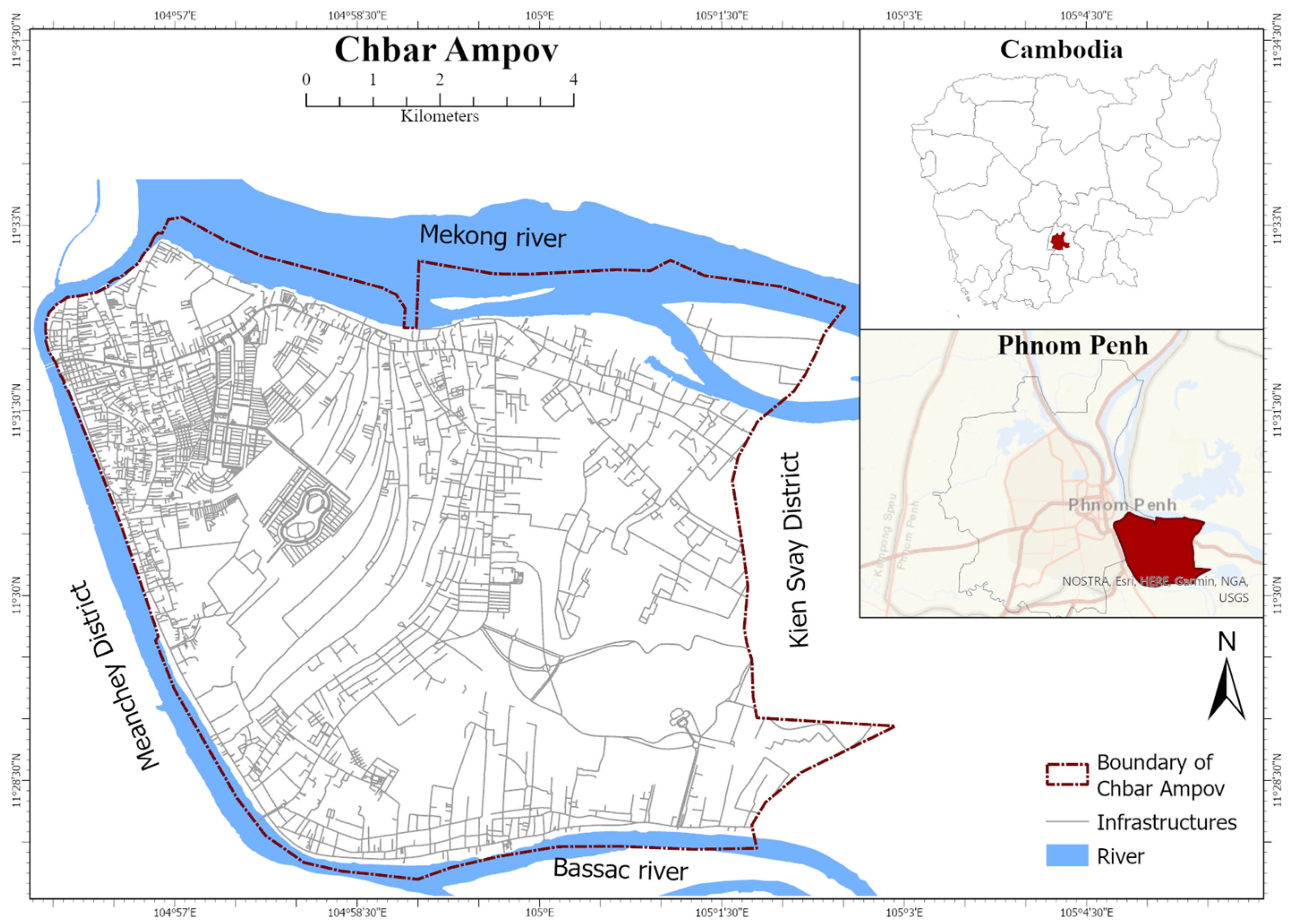
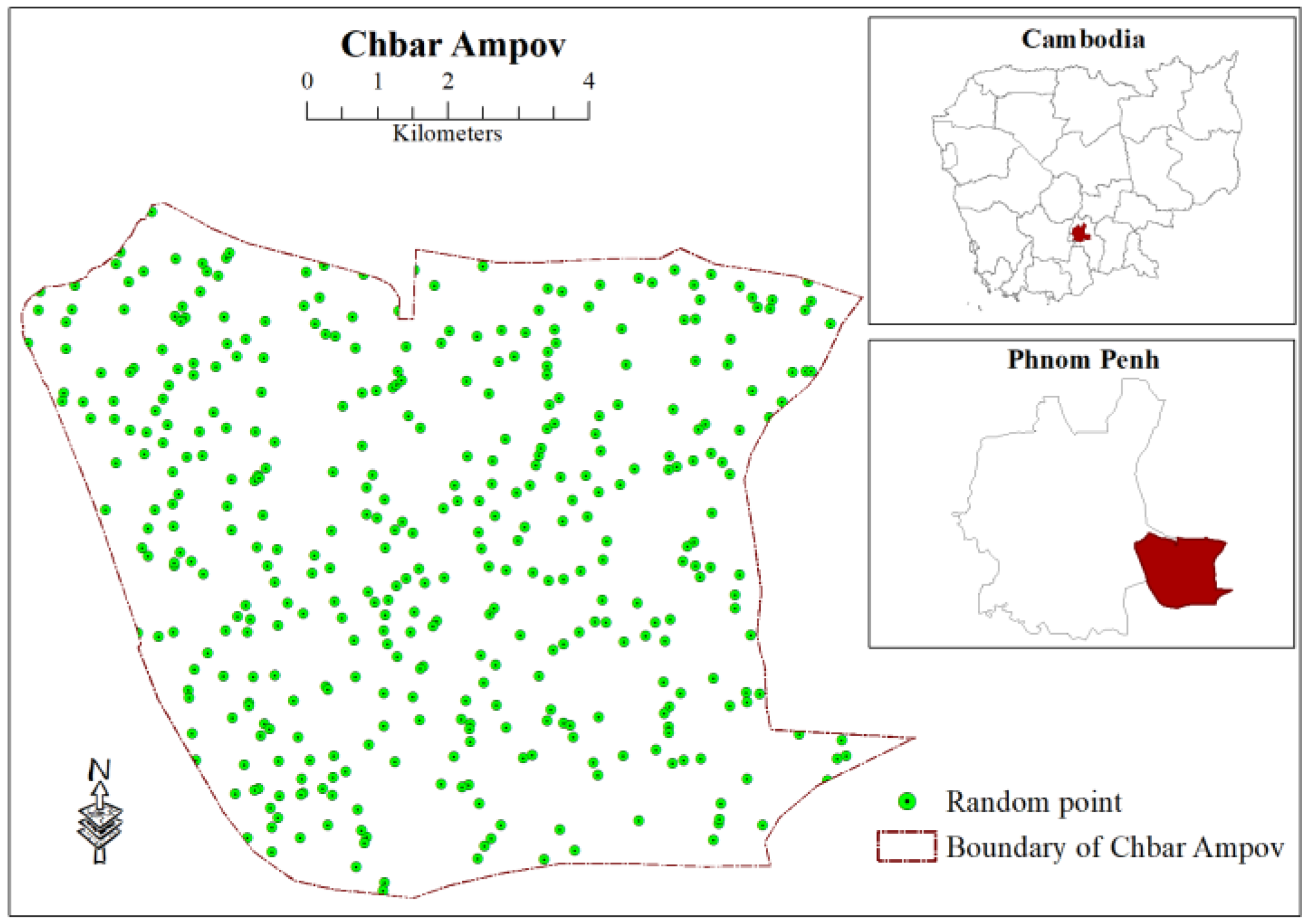
2.1. Study Area
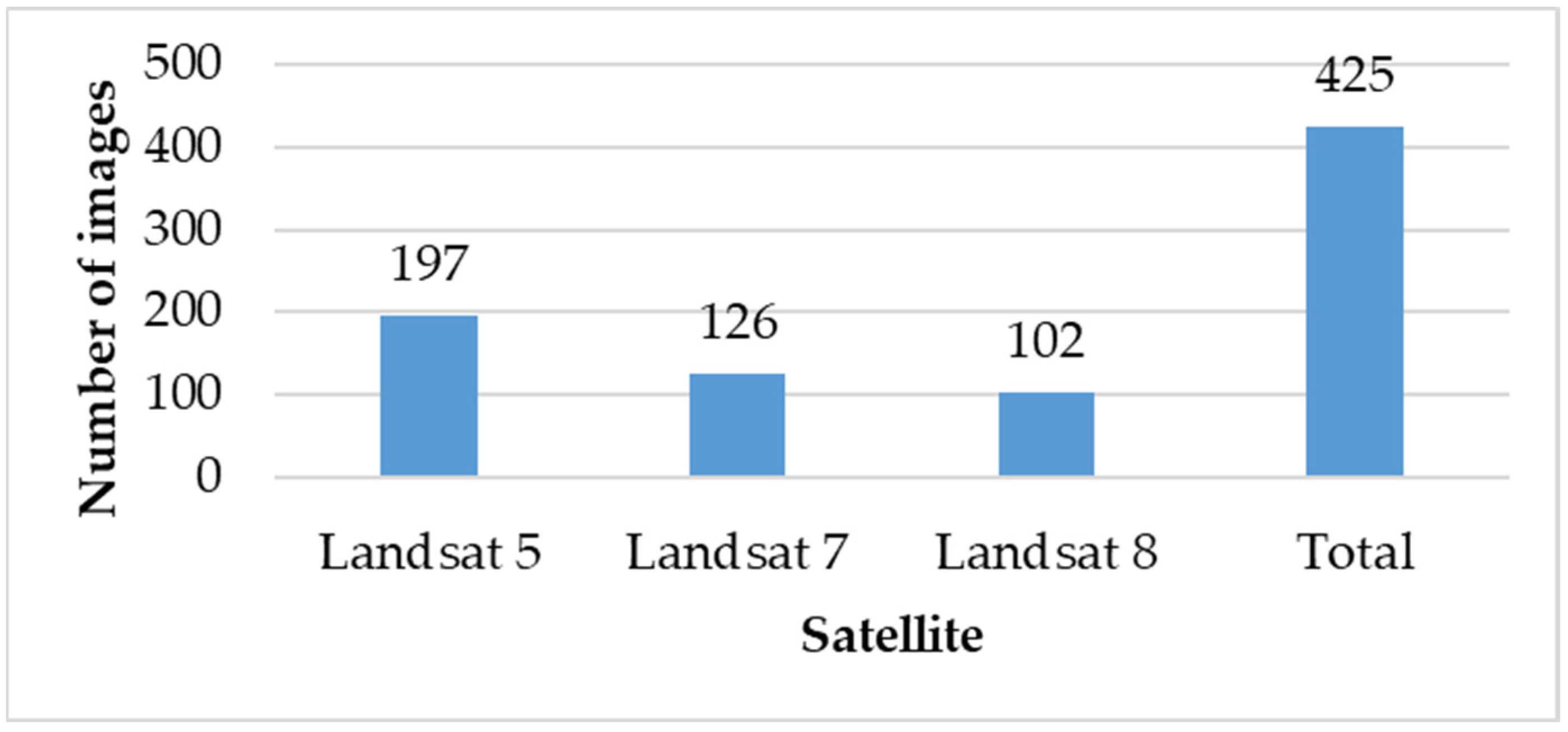
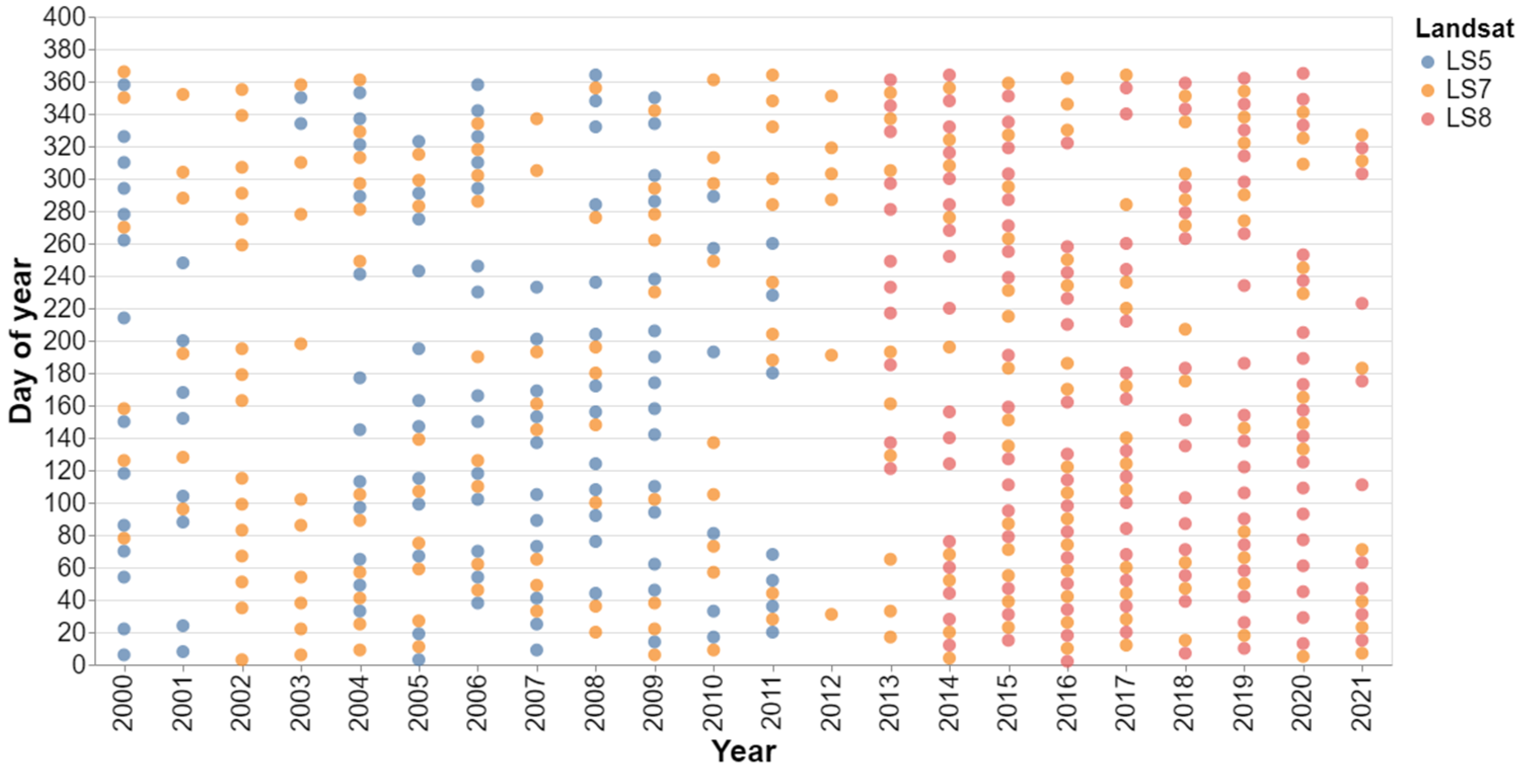
2.2. Data and Initial Processing
2.3. Spectral Indices Retrieval
2.4. Proportion of Vegetation and Emissivity Calculation
2.5. LST Retrieval
2.6. Statistical Analysis
2.7. Visual Interpretation
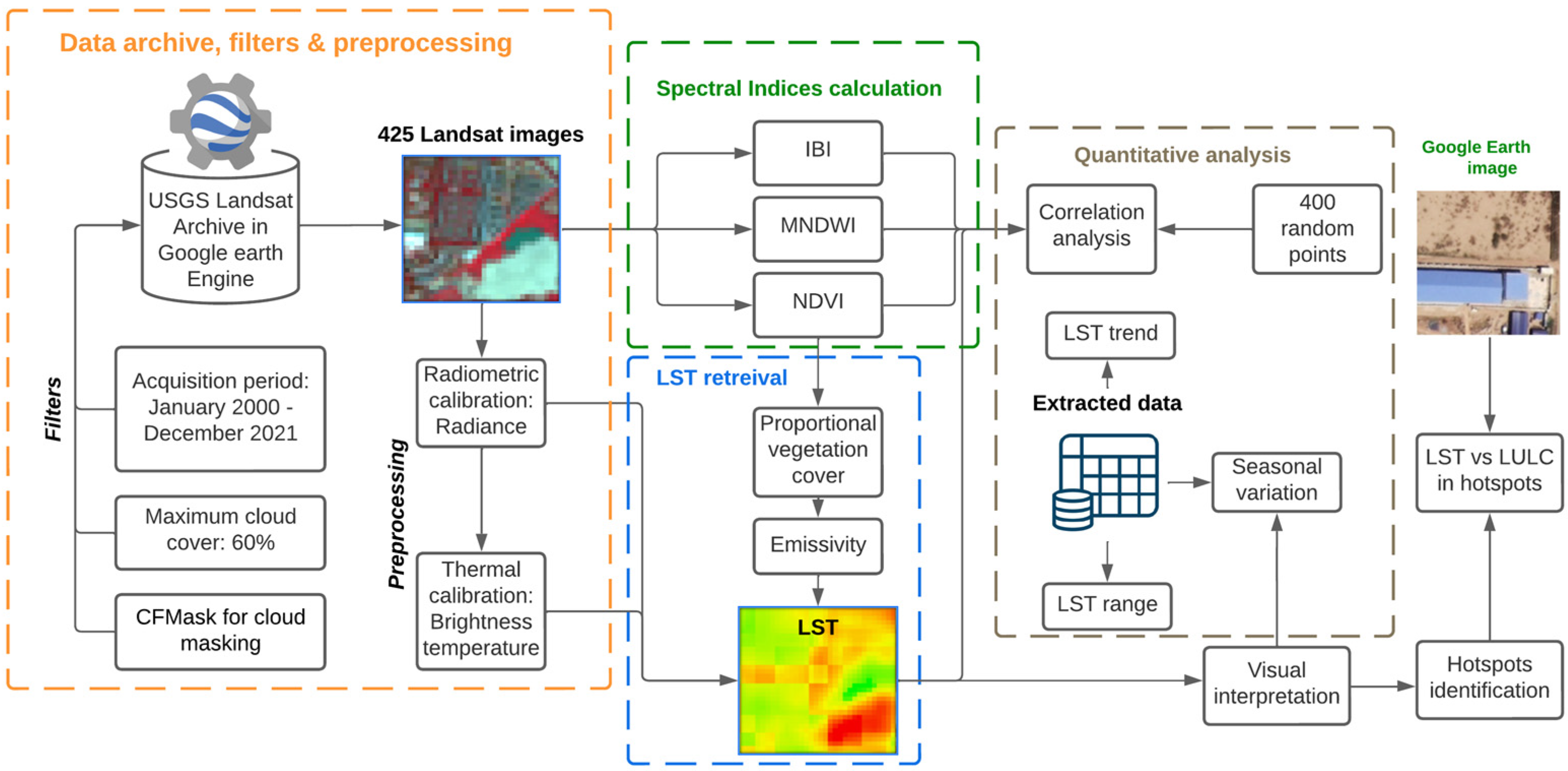
2.8. Overview of the Overall Methodology
3. Results
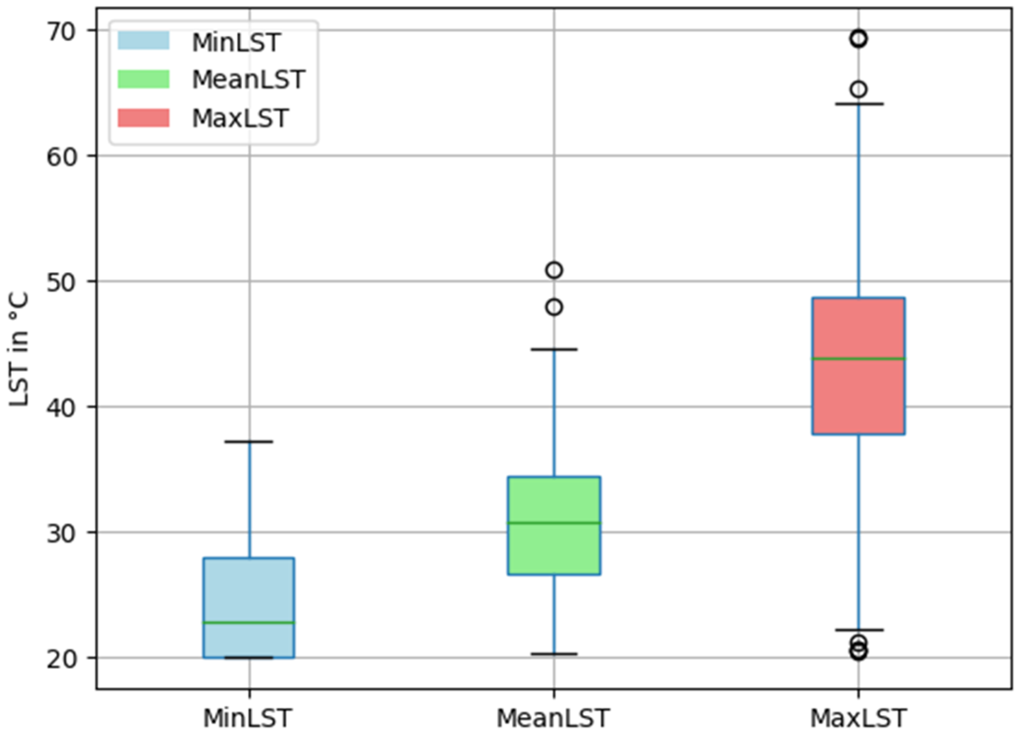
3.1. LST Distribution and Range
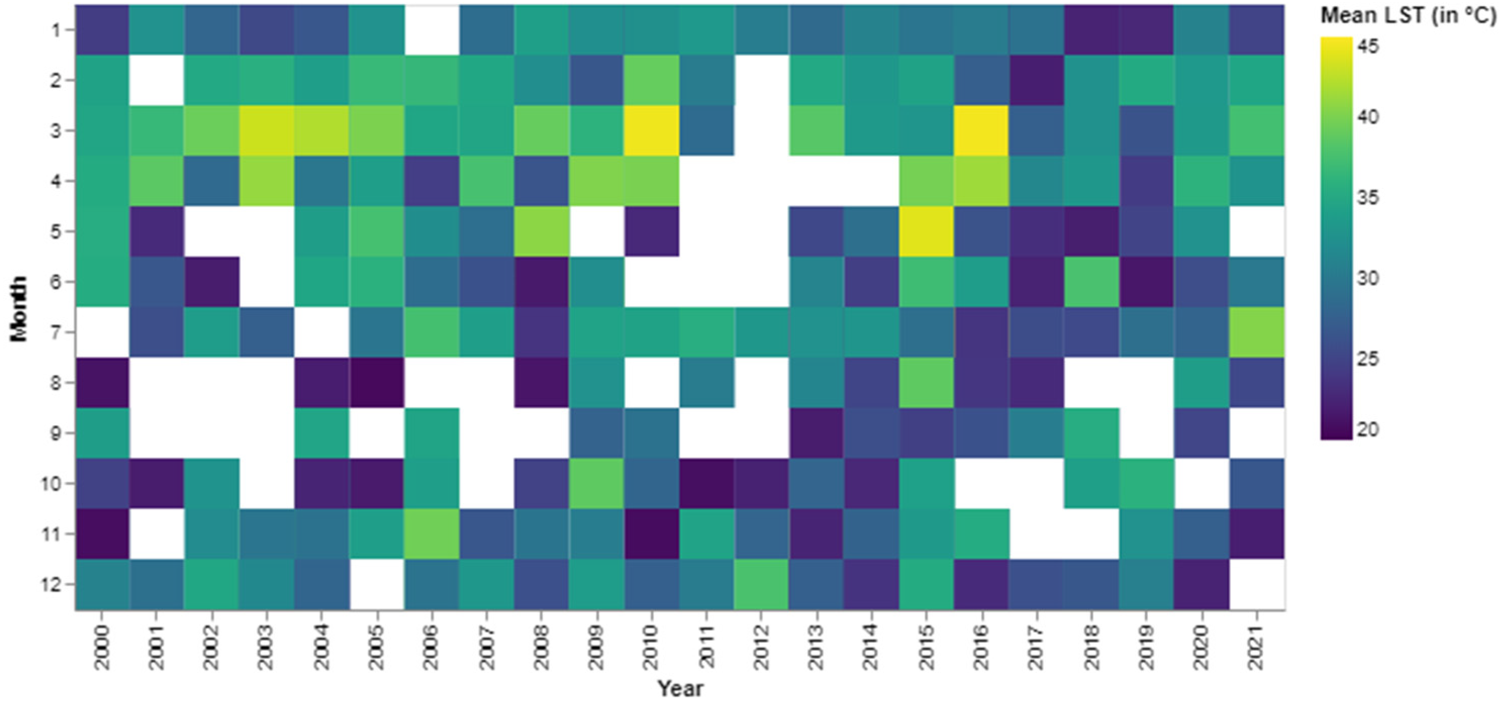
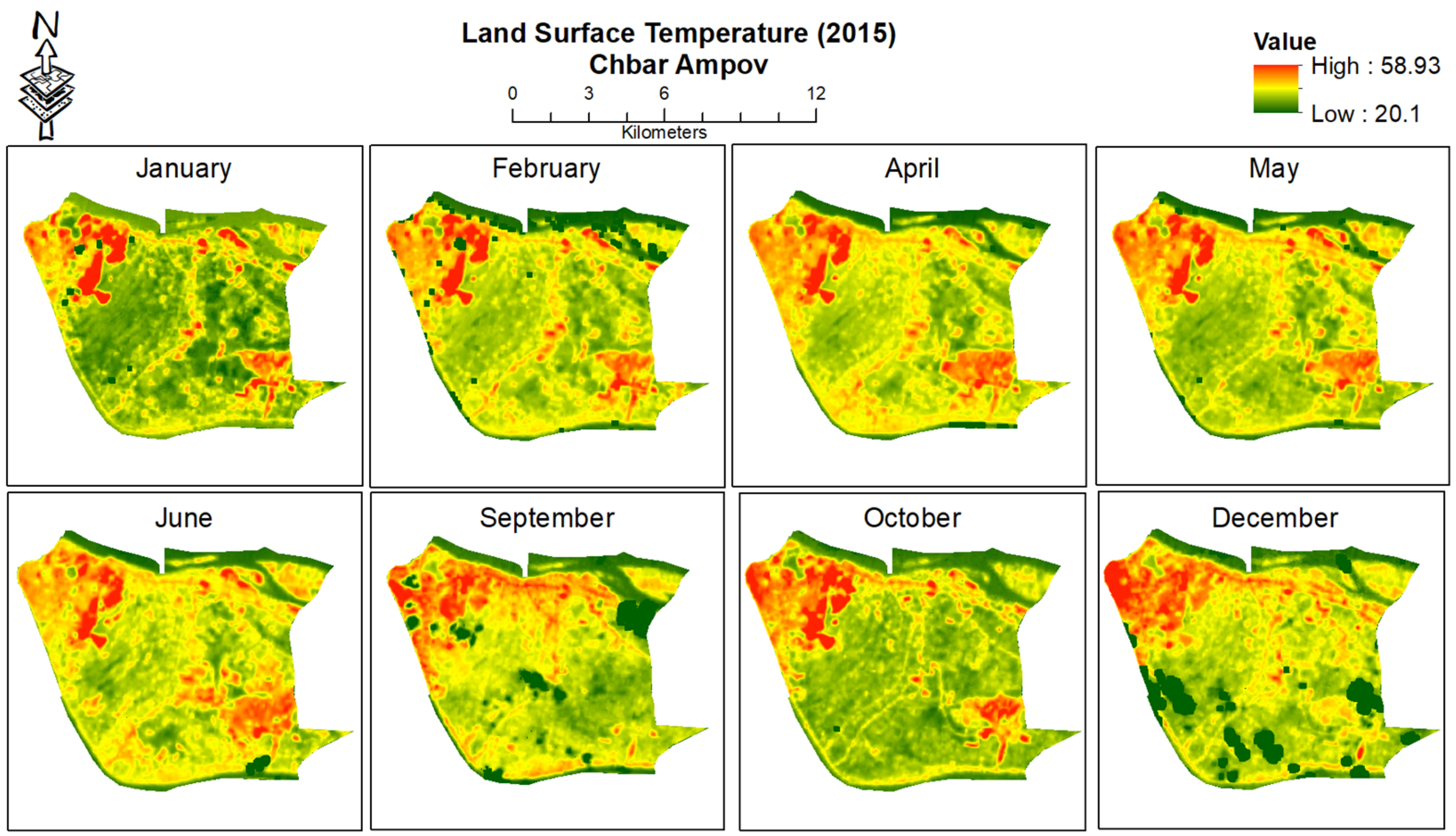
3.1.1. Seasonal Trends
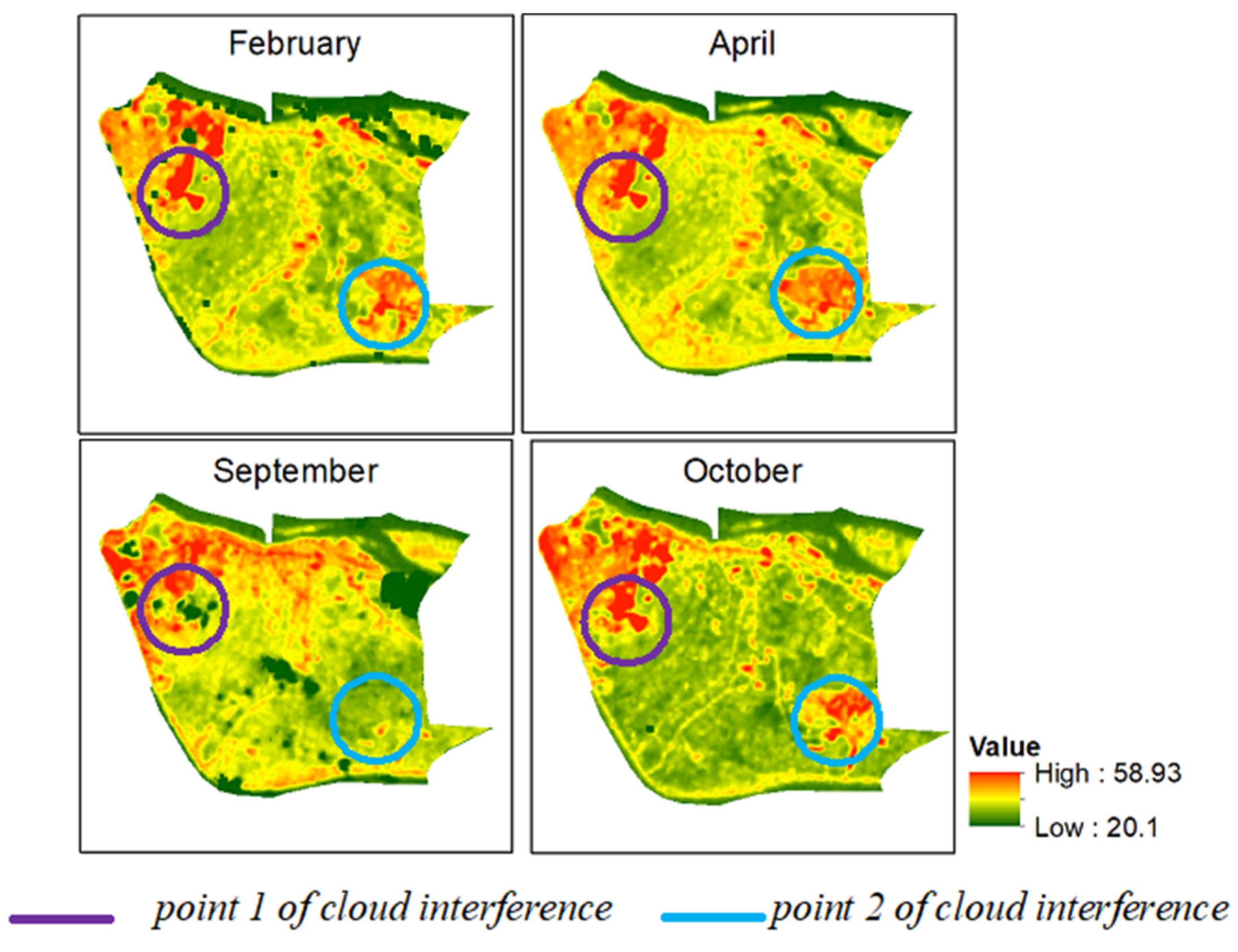
3.1.2. Anomalies and Extreme Events
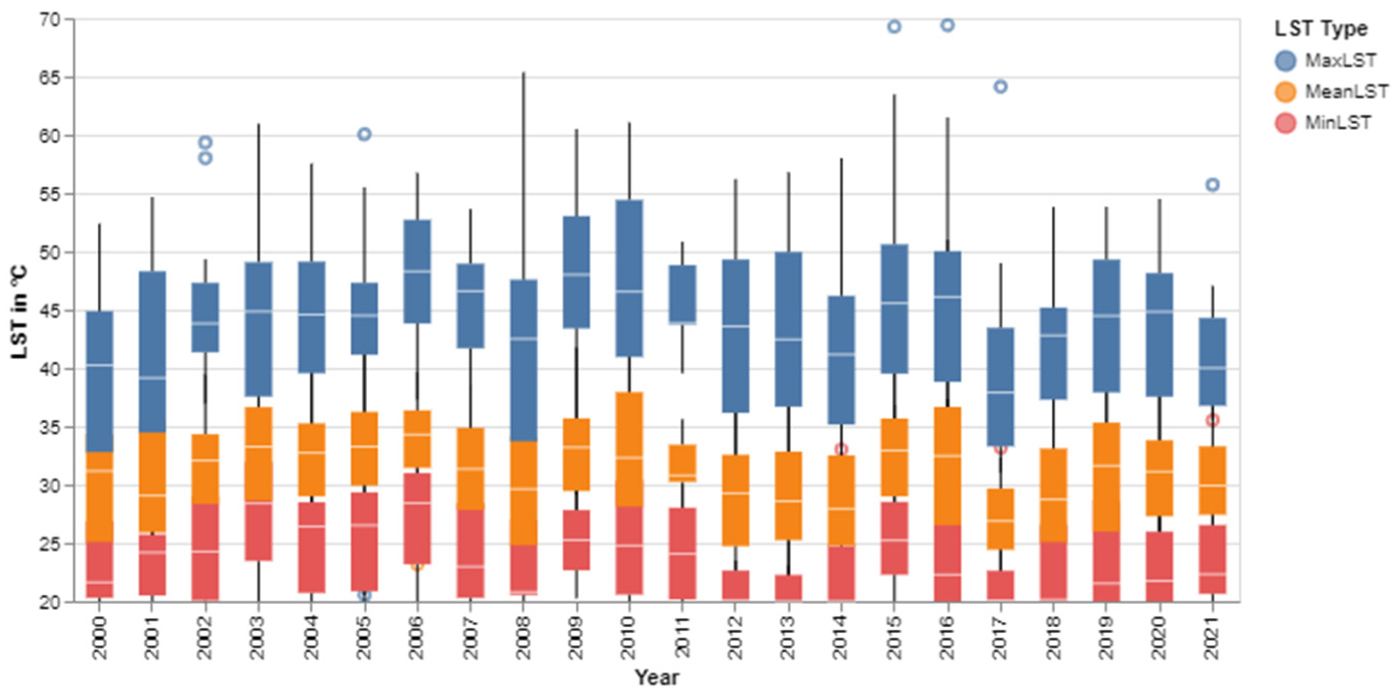
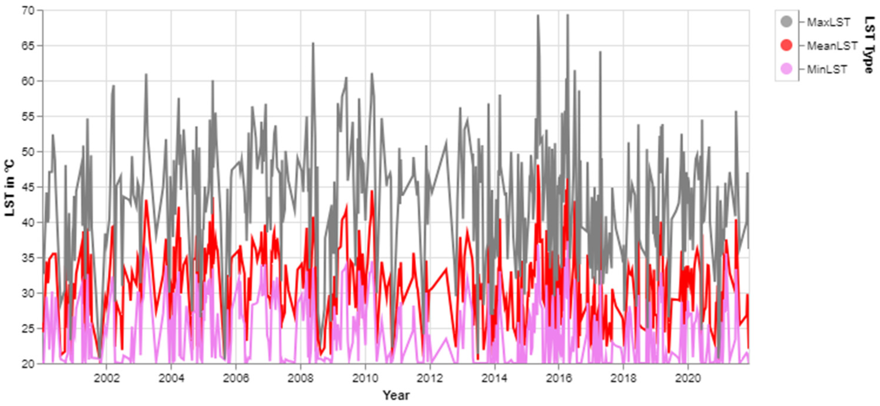
3.2. Consistency of LST Range and Trend of LST
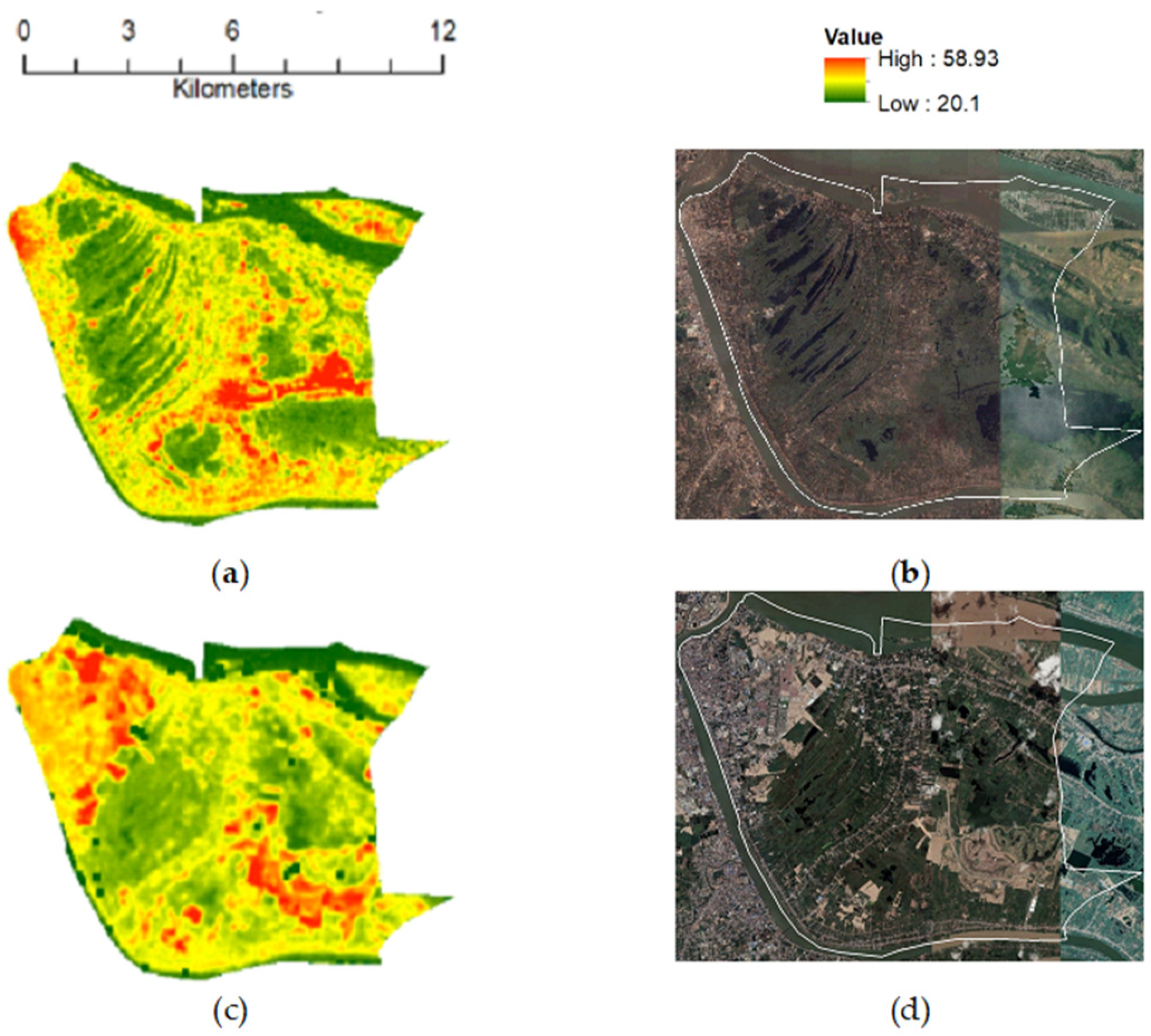
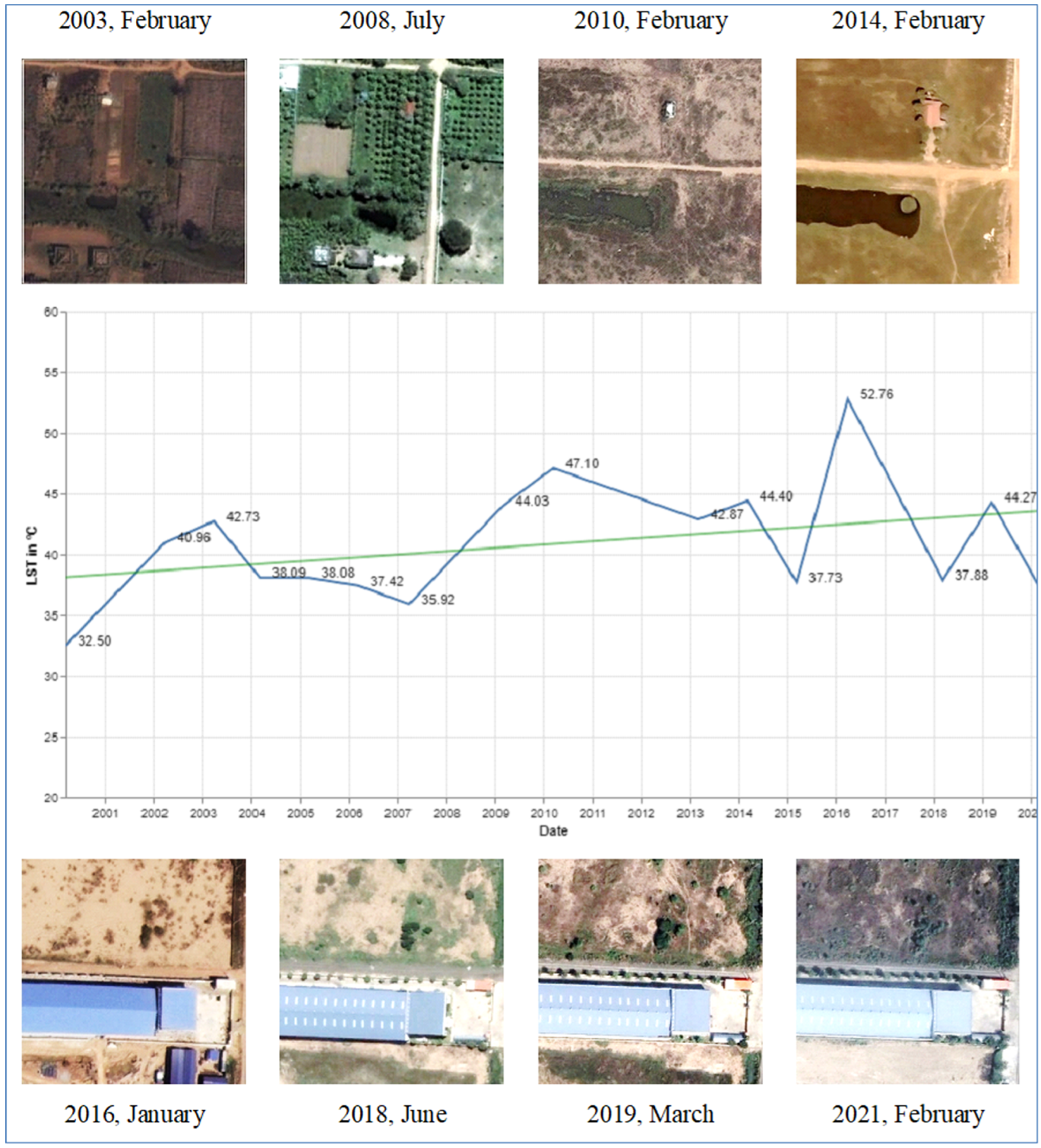
3.3. Results from the Visual Interpretations
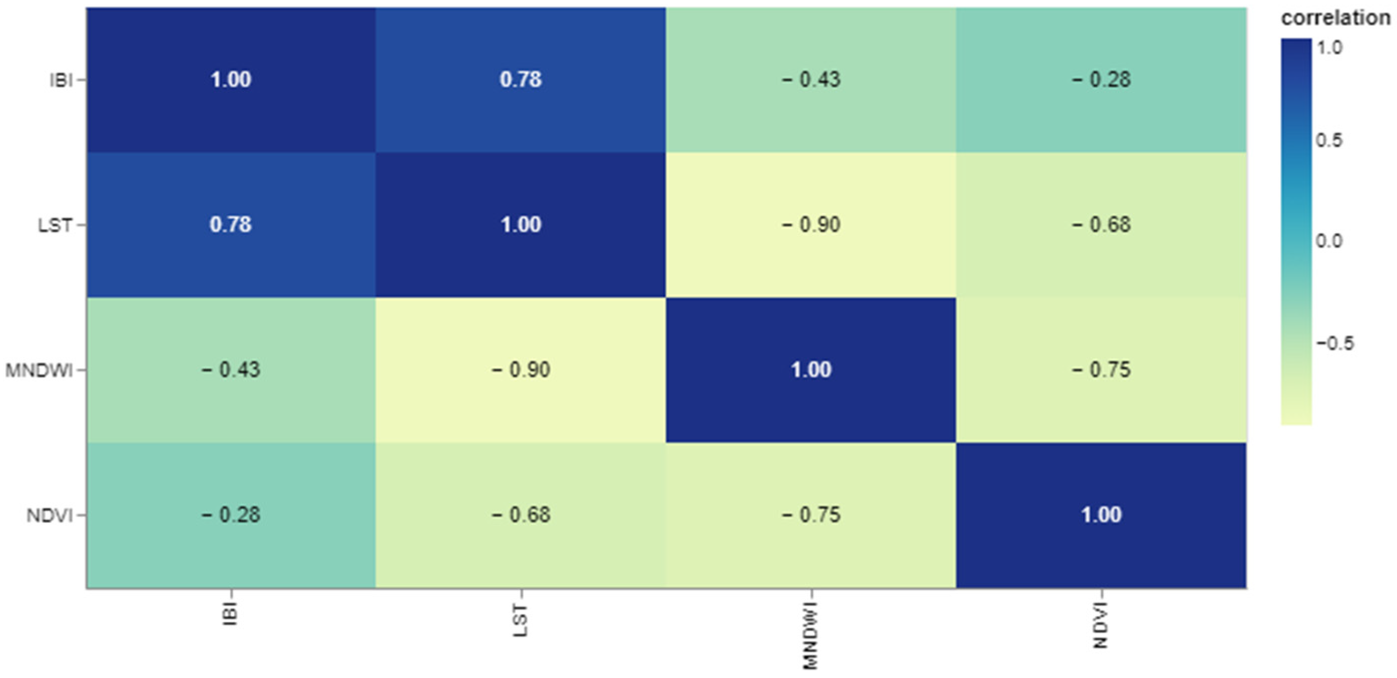
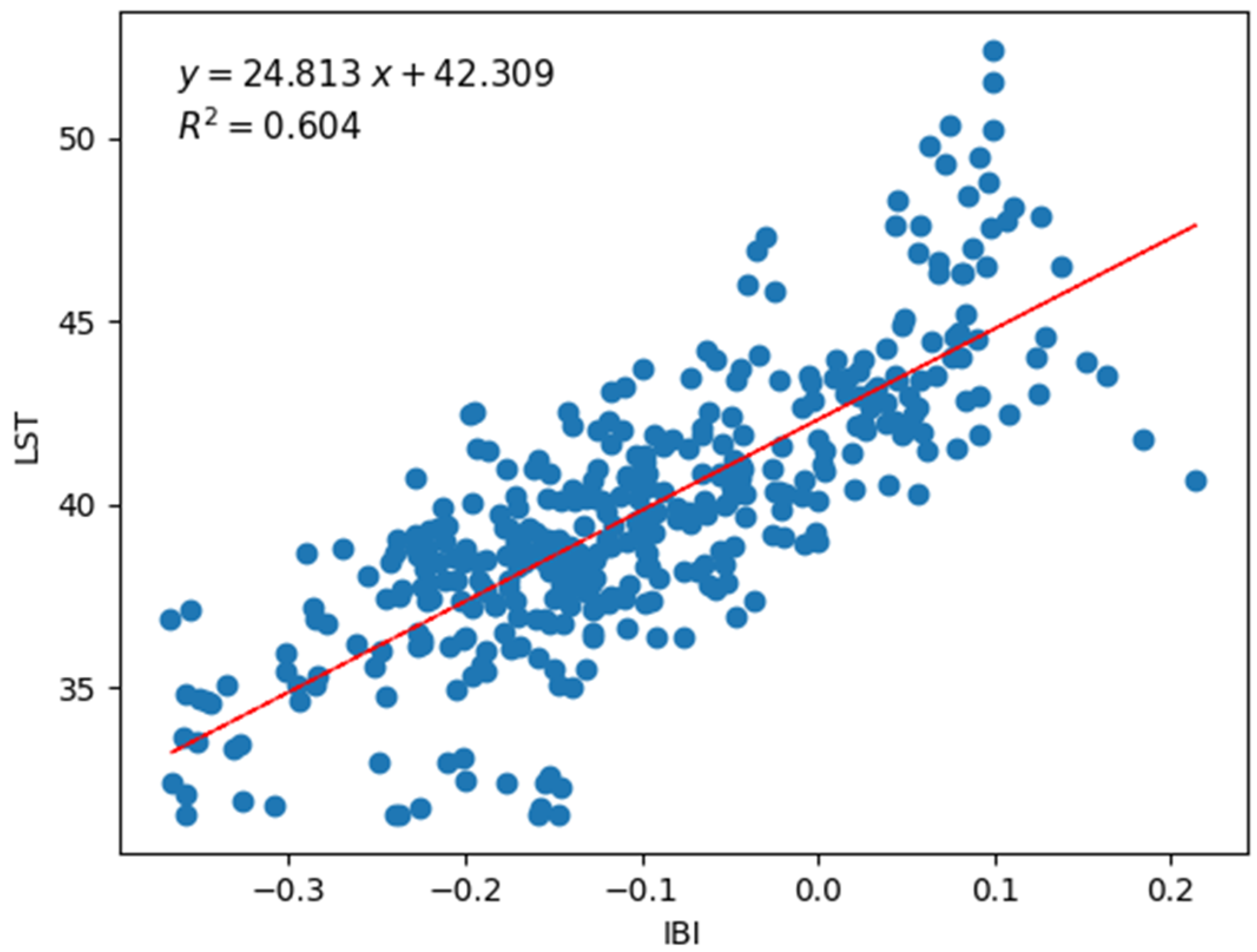
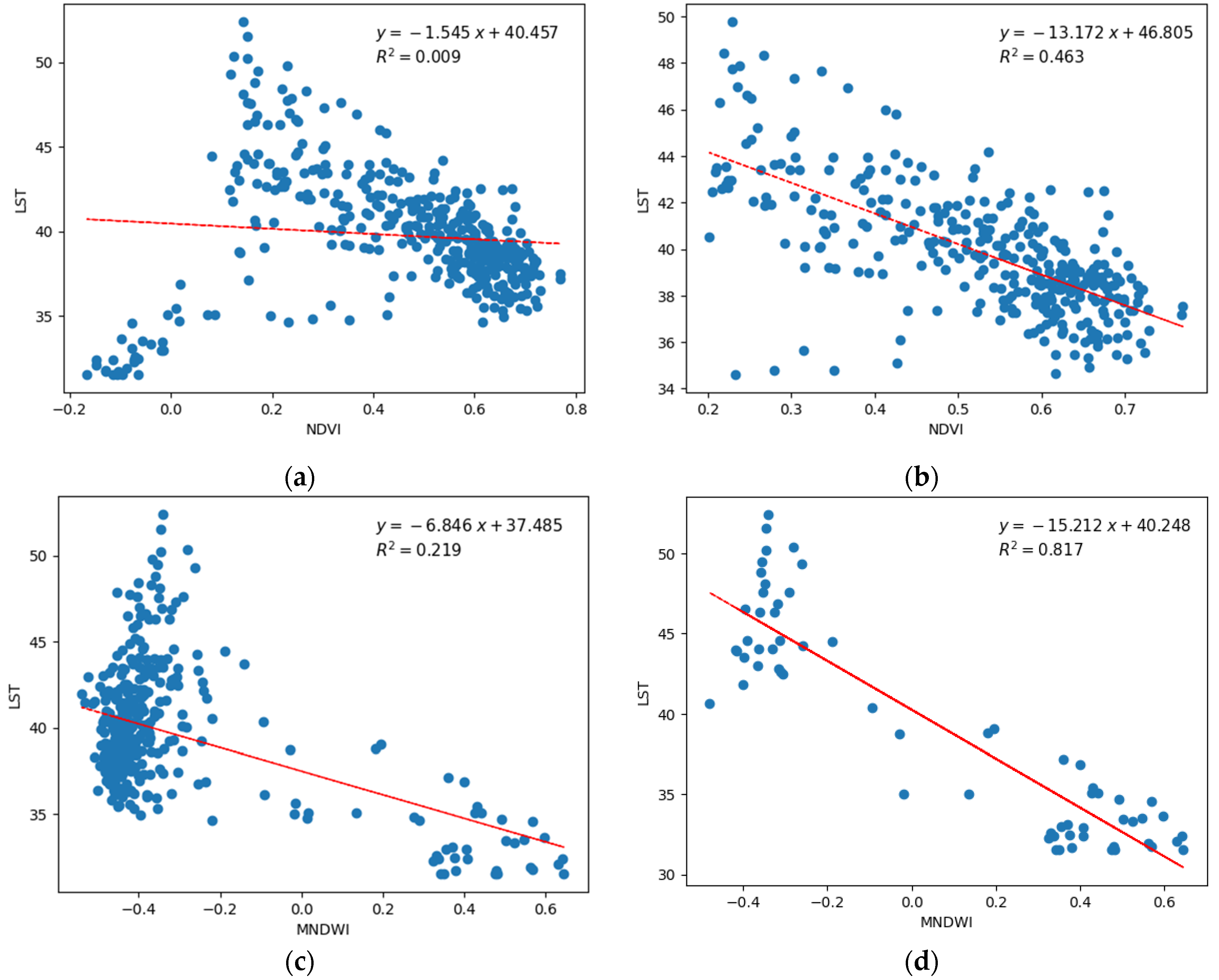
3.4. Correlation between LST and Different Land Covers
4. Discussion
5. Conclusions and Outlook
Author Contributions
Funding
Data Availability Statement
Acknowledgments
Conflicts of Interest
Appendix A

Appendix B

Appendix C

| Section | Content | Type of LST Value |
|---|---|---|
| 3.1 | Boxplot (Figure 5) | Minimum, mean and maximum |
| 3.1 | Calendar heatmap (Figure 6) | Mean |
| 3.2 | Boxplot (Figure 7) | Minimum, mean and maximum |
| 3.2 | Line chart (Figure 8) | Minimum, mean and maximum |
| 3.3 | Seasonal variability map (Figure 9) | Absolute |
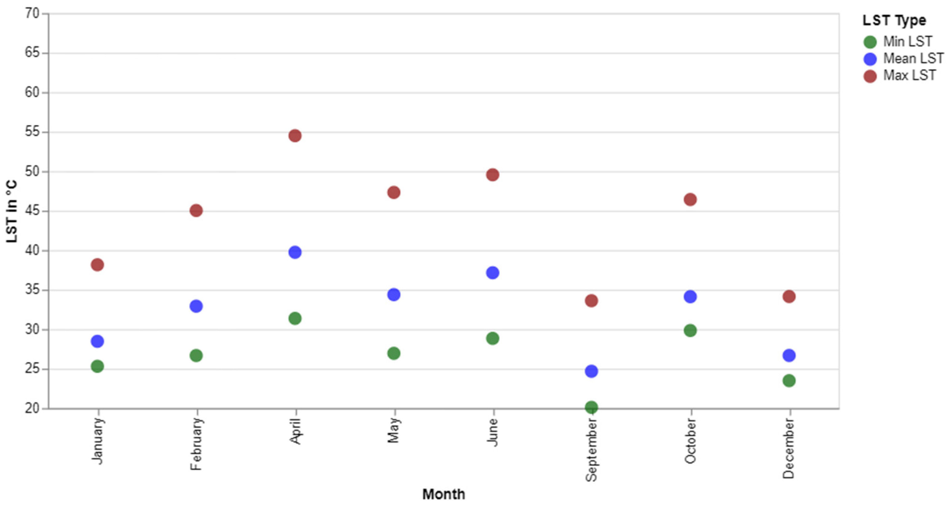
| 3.3 | Point chart (Figure 10) | Minimum, mean and maximum |
| 3.3 | Cloud contamination example map (Figure 11) | Absolute |
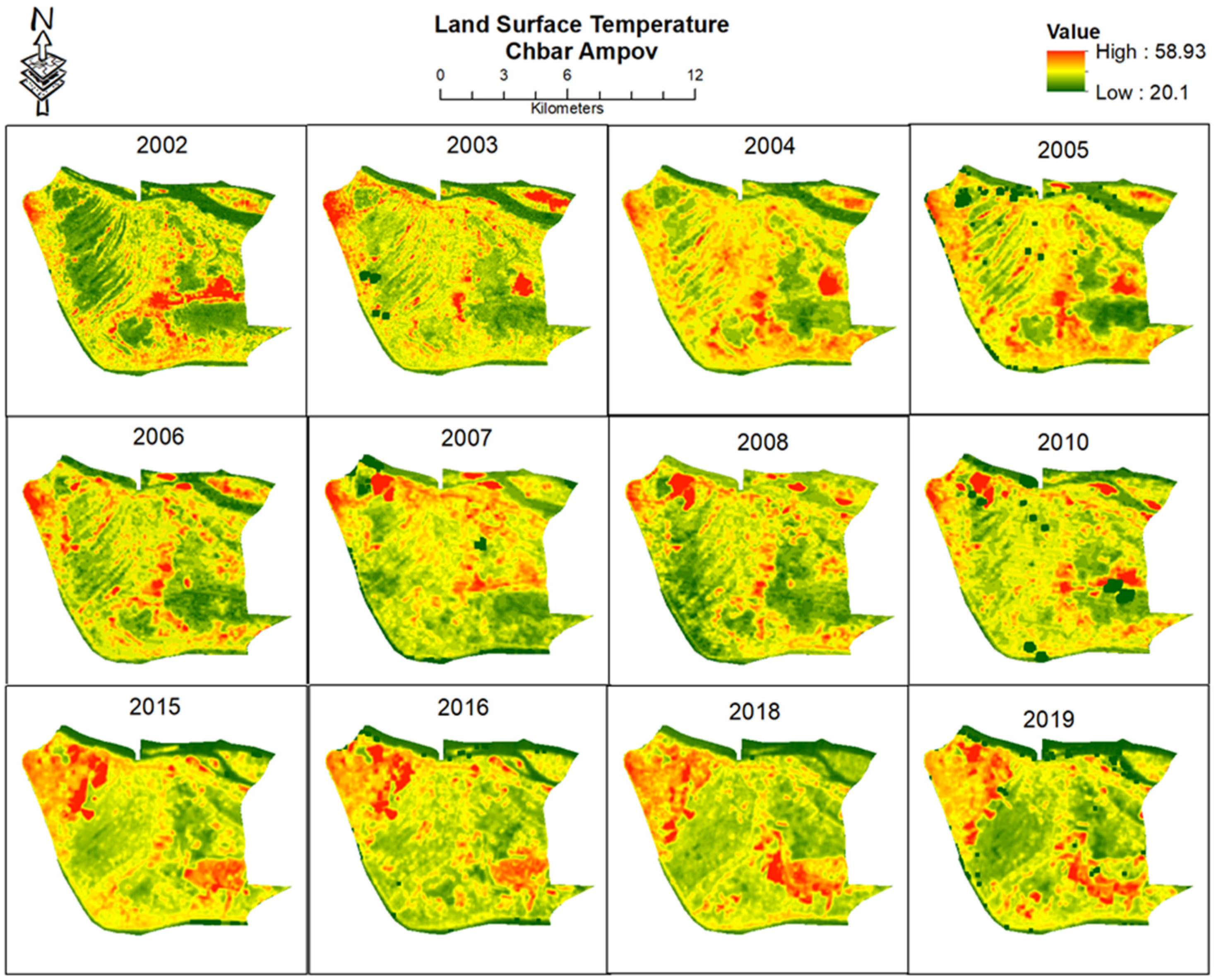
| 3.3 | Visual timeline of LST (Figure 12) | Absolute |
| 3.3 | Visible connection between LST (in °C) and LULC changes elaborating spatial changes (Figure 13) | Absolute |
| 3.3 | Point specific LST and LULC connection (Figure 14) | Absolute |
| 3.4 | LST and LULC correlation scatterplots (Figure 16 and Figure 17) | Absolute |
References
- Weng, Q. Thermal Infrared Remote Sensing for Urban Climate and Environmental Studies: Methods, Applications, and Trends. ISPRS J. Photogramm. Remote Sens. 2009, 64, 335–344. [Google Scholar] [CrossRef]
- NASA. Land Surface Temperature. NASA Earth Observatory. National Aeronautics and Space Administration (NASA). 2024. Available online: https://earthobservatory.nasa.gov/global-maps/MOD_LSTD_M (accessed on 18 March 2024).
- Yang, C.; Yan, F.; Zhang, S. Comparison of Land Surface and Air Temperatures for Quantifying Summer and Winter Urban Heat Island in a Snow Climate City. J. Environ. Manag. 2020, 265, 110563. [Google Scholar] [CrossRef]
- Xiang, Y.; Zheng, B.; Bedra, K.B.; Ouyang, Q.; Liu, J.; Zheng, J. Spatial and Seasonal Differences between near Surface Air Temperature and Land Surface Temperature for Urban Heat Island Effect Assessment. Urban Clim. 2023, 52, 101745. [Google Scholar] [CrossRef]
- Good, E.J.; Aldred, F.M.; Ghent, D.J.; Veal, K.L.; Jimenez, C. An Analysis of the Stability and Trends in the LST_cci Land Surface Temperature Datasets Over Europe. Earth Space Sci. 2022, 9, e2022EA002317. [Google Scholar] [CrossRef]
- Liang, S.; Wang, J. Chapter 7—Land Surface Temperature and Thermal Infrared Emissivity. In Advanced Remote Sensing, 2nd ed.; Liang, S., Wang, J., Eds.; Academic Press: Cambridge, MA, USA, 2020; pp. 251–295. [Google Scholar]
- Oke, T.R.; Cleugh, H.A. Urban Heat Storage Derived as Energy Balance Residuals. Bound.-Layer Meteorol. 1987, 39, 233–245. [Google Scholar] [CrossRef]
- Arnfield, A.J. Two Decades of Urban Climate Research: A Review of Turbulence, Exchanges of Energy and Water, and the Urban Heat Island. Int. J. Climatol. 2003, 23, 1–26. [Google Scholar] [CrossRef]
- Santamouris, M. (Ed.) Energy and Climate in the Urban Built Environment; James & James: London, UK, 2001; ISBN 978-1-873936-90-0. [Google Scholar]
- Kovats, R.S.; Hajat, S. Heat Stress and Public Health: A Critical Review. Annu. Rev. Public Health 2008, 29, 41–55. [Google Scholar] [CrossRef] [PubMed]
- Hondula, D.M.; Georgescu, M.; Balling, R.C. Challenges Associated with Projecting Urbanization-Induced Heat-Related Mortality. Sci. Total Environ. 2014, 490, 538–544. [Google Scholar] [CrossRef]
- Patz, J.A.; Campbell-Lendrum, D.; Holloway, T.; Foley, J.A. Impact of Regional Climate Change on Human Health. Nature 2005, 438, 310–317. [Google Scholar] [CrossRef]
- Santamouris, M. On the Energy Impact of Urban Heat Island and Global Warming on Buildings. Energy Build. 2014, 82, 100–113. [Google Scholar] [CrossRef]
- Zhang, P.; Imhoff, M.L.; Wolfe, R.E.; Bounoua, L. Characterizing Urban Heat Islands of Global Settlements Using MODIS and Nighttime Lights Products. Can. J. Remote Sens. 2010, 36, 185–196. [Google Scholar] [CrossRef]
- Jacob, D.J.; Winner, D.A. Effect of Climate Change on Air Quality. Atmos. Environ. 2009, 43, 51–63. [Google Scholar] [CrossRef]
- Grimm, N.B.; Faeth, S.H.; Golubiewski, N.E.; Redman, C.L.; Wu, J.; Bai, X.; Briggs, J.M. Global Change and the Ecology of Cities. Science 2008, 319, 756–760. [Google Scholar] [CrossRef] [PubMed]
- Pickett, S.T.A.; Cadenasso, M.L.; Grove, J.M. Resilient Cities: Meaning, Models, and Metaphor for Integrating the Ecological, Socio-Economic, and Planning Realms. Landsc. Urban Plan. 2004, 69, 369–384. [Google Scholar] [CrossRef]
- Akbari, H.; Pomerantz, M.; Taha, H. Cool Surfaces and Shade Trees to Reduce Energy Use and Improve Air Quality in Urban Areas. Sol. Energy 2001, 70, 295–310. [Google Scholar] [CrossRef]
- Nagler, P.; Glenn, E.; Nguyen, U.; Scott, R.; Doody, T. Estimating Riparian and Agricultural Actual Evapotranspiration by Reference Evapotranspiration and MODIS Enhanced Vegetation Index. Remote Sens. 2013, 5, 3849–3871. [Google Scholar] [CrossRef]
- Box, G.E.P.; Jenkins, G.M.; Reinsel, G.C.; Ljung, G.M. Time Series Analysis: Forecasting and Control, 5th ed.; Wiley Series in Probability and Statistics; Wiley: Hoboken, NJ, USA, 2016. [Google Scholar]
- Erell, E.; Pearlmutter, D.; Williamson, T.J. Urban Microclimate: Designing the Spaces between Buildings, 1st ed.; Earthscan: London, UK; Washington, DC, USA, 2011. [Google Scholar]
- Santamouris, M. Cooling the Cities—A Review of Reflective and Green Roof Mitigation Technologies to Fight Heat Island and Improve Comfort in Urban Environments. Sol. Energy 2014, 103, 682–703. [Google Scholar] [CrossRef]
- Hajat, S.; O’Connor, M.; Kosatsky, T. Health Effects of Hot Weather: From Awareness of Risk Factors to Effective Health Protection. Lancet 2010, 375, 856–863. [Google Scholar] [CrossRef] [PubMed]
- Kleerekoper, L.; Van Esch, M.; Salcedo, T.B. How to Make a City Climate-Proof, Addressing the Urban Heat Island Effect. Resour. Conserv. Recycl. 2012, 64, 30–38. [Google Scholar] [CrossRef]
- Weng, Q.; Liu, H.; Liang, B.; Lu, D. The Spatial Variations of Urban Land Surface Temperatures: Pertinent Factors, Zoning Effect, and Seasonal Variability. IEEE J. Sel. Top. Appl. Earth Obs. Remote Sens. 2008, 1, 154–166. [Google Scholar] [CrossRef]
- Amiri, R.; Weng, Q.; Alimohammadi, A.; Alavipanah, S.K. Spatial–Temporal Dynamics of Land Surface Temperature in Relation to Fractional Vegetation Cover and Land Use/Cover in the Tabriz Urban Area, Iran. Remote Sens. Environ. 2009, 113, 2606–2626. [Google Scholar] [CrossRef]
- Carlson, T.N.; Gillies, R.R.; Perry, E.M. A Method to Make Use of Thermal Infrared Temperature and NDVI Measurements to Infer Surface Soil Water Content and Fractional Vegetation Cover. Remote Sens. Rev. 1994, 9, 161–173. [Google Scholar] [CrossRef]
- Moran, M. Combining Multifrequency Microwave and Optical Data for Crop Management. Remote Sens. Environ. 1997, 61, 96–109. [Google Scholar] [CrossRef]
- Gillies, R.R.; Kustas, W.P.; Humes, K.S. A Verification of the “triangle” Method for Obtaining Surface Soil Water Content and Energy Fluxes from Remote Measurements of the Normalized Difference Vegetation Index (NDVI) and Surface e. Int. J. Remote Sens. 1997, 18, 3145–3166. [Google Scholar] [CrossRef]
- Sandholt, I.; Rasmussen, K.; Andersen, J. A Simple Interpretation of the Surface Temperature/Vegetation Index Space for Assessment of Surface Moisture Status. Remote Sens. Environ. 2002, 79, 213–224. [Google Scholar] [CrossRef]
- Xu, H. Modification of Normalised Difference Water Index (NDWI) to Enhance Open Water Features in Remotely Sensed Imagery. Int. J. Remote Sens. 2006, 27, 3025–3033. [Google Scholar] [CrossRef]
- Xu, H. A New Index for Delineating Built-up Land Features in Satellite Imagery. Int. J. Remote Sens. 2008, 29, 4269–4276. [Google Scholar] [CrossRef]
- Karakuş, C.B. The Impact of Land Use/Land Cover (LULC) Changes on Land Surface Temperature in Sivas City Center and Its Surroundings and Assessment of Urban Heat Island. Asia-Pac. J. Atmos. Sci. 2019, 55, 669–684. [Google Scholar] [CrossRef]
- Saha, S.; Saha, A.; Das, M.; Saha, A.; Sarkar, R.; Das, A. Analyzing Spatial Relationship between Land Use/Land Cover (LULC) and Land Surface Temperature (LST) of Three Urban Agglomerations (UAs) of Eastern India. Remote Sens. Appl. Soc. Environ. 2021, 22, 100507. [Google Scholar] [CrossRef]
- Fatemi, M.; Narangifard, M. Monitoring LULC Changes and Its Impact on the LST and NDVI in District 1 of Shiraz City. Arab. J. Geosci. 2019, 12, 127. [Google Scholar] [CrossRef]
- Zhang, F.; Tiyip, T.; Kung, H.; Johnson, V.C.; Maimaitiyiming, M.; Zhou, M.; Wang, J. Dynamics of Land Surface Temperature (LST) in Response to Land Use and Land Cover (LULC) Changes in the Weigan and Kuqa River Oasis, Xinjiang, China. Arab. J. Geosci. 2016, 9, 499. [Google Scholar] [CrossRef]
- Peng, X.; Wu, W.; Zheng, Y.; Sun, J.; Hu, T.; Wang, P. Correlation Analysis of Land Surface Temperature and Topographic Elements in Hangzhou, China. Sci. Rep. 2020, 10, 10451. [Google Scholar] [CrossRef] [PubMed]
- Murtaza, K.O.; Shafai, S.; Shahid, P.; Romshoo, S.A. Understanding the Linkages between Spatio-Temporal Urban Land System Changes and Land Surface Temperature in Srinagar City, India, Using Image Archives from Google Earth Engine. Env. Sci. Pollut. Res. 2023, 30, 107281–107295. [Google Scholar] [CrossRef] [PubMed]
- Lin, J.; Wei, K.; Guan, Z. Exploring the Connection between Morphological Characteristic of Built-Up Areas and Surface Heat Islands Based on MSPA. Urban Clim. 2024, 53, 101764. [Google Scholar] [CrossRef]
- Saha, J.; Ria, S.S.; Sultana, J.; Shima, U.A.; Hasan Seyam, M.M.; Rahman, M.M. Assessing Seasonal Dynamics of Land Surface Temperature (LST) and Land Use Land Cover (LULC) in Bhairab, Kishoreganj, Bangladesh: A Geospatial Analysis from 2008 to 2023. Case Stud. Chem. Environ. Eng. 2024, 9, 100560. [Google Scholar] [CrossRef]
- Alfieri, S.M.; De Lorenzi, F.; Menenti, M. Mapping Air Temperature Using Time Series Analysis of LST: The SINTESI Approach. Nonlin. Process. Geophys. 2013, 20, 513–527. [Google Scholar] [CrossRef]
- Fu, P.; Weng, Q. A Time Series Analysis of Urbanization Induced Land Use and Land Cover Change and Its Impact on Land Surface Temperature with Landsat Imagery. Remote Sens. Environ. 2016, 175, 205–214. [Google Scholar] [CrossRef]
- Nill, L.; Ullmann, T.; Kneisel, C.; Sobiech-Wolf, J.; Baumhauer, R. Assessing Spatiotemporal Variations of Landsat Land Surface Temperature and Multispectral Indices in the Arctic Mackenzie Delta Region between 1985 and 2018. Remote Sens. 2019, 11, 2329. [Google Scholar] [CrossRef]
- Asif, F.; Beckwith, L.; Ngin, C. People and Politics: Urban Climate Resilience in Phnom Penh, Cambodia. Front. Sustain. Cities 2023, 4, 972173. [Google Scholar] [CrossRef]
- Asia. (City District, Cambodia)—Population Statistics, Charts, Map and Location. 2024. Available online: https://www.citypopulation.de/en/cambodia/phnompenh/admin/1212__chbar_ampov/ (accessed on 18 March 2024).
- Phnom Penh Climate (Cambodia). Phnom Penh Climate: Weather Phnom Penh & Temperature by Month. 2024. Available online: https://en.climate-data.org/asia/cambodia/phnom-penh/phnom-penh-4857/ (accessed on 18 March 2024).
- Touch, S.; Likitlersuang, S.; Pipatpongsa, T. 3D Geological Modelling and Geotechnical Characteristics of Phnom Penh Subsoils in Cambodia. Eng. Geol. 2014, 178, 58–69. [Google Scholar] [CrossRef]
- Phnom Penh (Bassac). Regional Flood Management and Mitigation Centre. Mekong River Commision. 2024. Available online: http://ffw.mrcmekong.org/stations.php?StCode=PPB&StName=Phnom%20Penh%20(Bassac) (accessed on 18 March 2024).
- Bunleng, S.; Katzschner, L. Will Cities Survive? Urban Climate Recommendations for Urban Planning in Phnom Penh, Cambodia. In Proceedings of the PLEA SANTIAGO 2022W, Santiago, Chile, 22–25 November 2022. [Google Scholar]
- GEE. Landsat Collections in Earth Engine|Earth Engine Data Catalog|Google for Developers. Google Earth Engine. Google. 2024. Available online: https://developers.google.com/earth-engine/datasets/catalog/landsat (accessed on 18 March 2024).
- Foga, S.; Scaramuzza, P.L.; Guo, S.; Zhu, Z.; Dilley, R.D.; Beckmann, T.; Schmidt, G.L.; Dwyer, J.L.; Joseph Hughes, M.; Laue, B. Cloud Detection Algorithm Comparison and Validation for Operational Landsat Data Products. Remote Sens. Environ. 2017, 194, 379–390. [Google Scholar] [CrossRef]
- Rouse, J.W., Jr.; Haas, R.H.; Schell, J.A.; Deering, D.W. Monitoring the Vernal Advancement and Retrogradation (Green Wave Effect) of Natural Vegetation (No. NASA-CR-132982); NTRS: Washington, DC, USA, 1973.
- Carlson, T.N.; Ripley, D.A. On the Relation between NDVI, Fractional Vegetation Cover, and Leaf Area Index. Remote Sens. Environ. 1997, 62, 241–252. [Google Scholar] [CrossRef]
- Sobrino, J.A.; Jimenez-Munoz, J.C.; Soria, G.; Romaguera, M.; Guanter, L.; Moreno, J.; Plaza, A.; Martinez, P. Land Surface Emissivity Retrieval From Different VNIR and TIR Sensors. IEEE Trans. Geosci. Remote Sens. 2008, 46, 316–327. [Google Scholar] [CrossRef]
- Li, Z.-L.; Tang, B.-H.; Wu, H.; Ren, H.; Yan, G.; Wan, Z.; Trigo, I.F.; Sobrino, J.A. Satellite-Derived Land Surface Temperature: Current Status and Perspectives. Remote Sens. Environ. 2013, 131, 14–37. [Google Scholar] [CrossRef]
- Jimenez-Munoz, J.C.; Cristobal, J.; Sobrino, J.A.; Soria, G.; Ninyerola, M.; Pons, X.; Pons, X. Revision of the Single-Channel Algorithm for Land Surface Temperature Retrieval From Landsat Thermal-Infrared Data. IEEE Trans. Geosci. Remote Sens. 2009, 47, 339–349. [Google Scholar] [CrossRef]
- Jimenez-Munoz, J.C.; Sobrino, J.A.; Skokovic, D.; Mattar, C.; Cristobal, J. Land Surface Temperature Retrieval Methods From Landsat-8 Thermal Infrared Sensor Data. IEEE Geosci. Remote Sens. Lett. 2014, 11, 1840–1843. [Google Scholar] [CrossRef]
- Chander, G.; Markham, B.L.; Helder, D.L. Summary of Current Radiometric Calibration Coefficients for Landsat MSS, TM, ETM+, and EO-1 ALI Sensors. Remote Sens. Environ. 2009, 113, 893–903. [Google Scholar] [CrossRef]
- Reducer Overview of Google Earth Engine Algorithms. Available online: https://developers.google.com/earth-engine/guides/reducers_intro (accessed on 5 November 2023).
- Simpson, R.B.; Zhou, B.; Alarcon Falconi, T.M.; Naumova, E.N. An Analecta of Visualizations for Foodborne Illness Trends and Seasonality. Sci Data 2020, 7, 346. [Google Scholar] [CrossRef] [PubMed]
- Liu, J.; Yang, L.; Zhou, H.; Wang, S. Impact of Climate Change on Hiking: Quantitative Evidence through Big Data Mining. Curr. Issues Tour. 2021, 24, 3040–3056. [Google Scholar] [CrossRef]
- Weng, Q. A Remote Sensing? GIS Evaluation of Urban Expansion and Its Impact on Surface Temperature in the Zhujiang Delta, China. Int. J. Remote Sens. 2001, 22, 1999–2014. [Google Scholar]
- Zhou, Y.; Yang, G.; Wang, S.; Wang, L.; Wang, F.; Liu, X. A New Index for Mapping Built-up and Bare Land Areas from Landsat-8 OLI Data. Remote Sens. Lett. 2014, 5, 862–871. [Google Scholar] [CrossRef]
- How Often do El Niño and La Niña Typically Occur? Climate Prediction Center—Enso FAQ. National Weather Service. 2024. Available online: https://web.archive.org/web/20090827143632/http:/www.cpc.noaa.gov/products/analysis_monitoring/ensostuff/ensofaq.shtml#HOWOFTEN (accessed on 18 March 2024).
- Peng, S.; Piao, S.; Ciais, P.; Friedlingstein, P.; Ottle, C.; Bréon, F.-M.; Nan, H.; Zhou, L.; Myneni, R.B. Surface Urban Heat Island Across 419 Global Big Cities. Environ. Sci. Technol. 2012, 46, 696–703. [Google Scholar] [CrossRef] [PubMed]
- Bonan, G.B. Ecological Climatology: Concepts and Applications, 3rd ed.; Cambridge University Press: New York, NY, USA, 2016; ISBN 978-1-107-04377-0. [Google Scholar]
- Zomer, R.J.; Trabucco, A.; Bossio, D.A.; Verchot, L.V. Climate Change Mitigation: A Spatial Analysis of Global Land Suitability for Clean Development Mechanism Afforestation and Reforestation. Agric. Ecosyst. Environ. 2008, 126, 67–80. [Google Scholar] [CrossRef]
- Wang, Q.; Wang, L.; Wei, C.; Jin, Y.; Li, Z.; Tong, X.; Atkinson, P.M. Filling Gaps in Landsat ETM+ SLC-off Images with Sentinel-2 MSI Images. Int. J. Appl. Earth Obs. Geoinf. 2021, 101, 102365. [Google Scholar] [CrossRef]
- Montanaro, M.; Barsi, J.; Lunsford, A.; Rohrbach, S.; Markham, B. Performance of the Thermal Infrared Sensor On-Board Landsat 8 over the First Year On-Orbit; Butler, J.J., Xiong, X., Gu, X., Eds.; SPIE: San Diego, CA, USA, 2014; p. 921817. [Google Scholar]
- Du, C.; Ren, H.; Qin, Q.; Meng, J.; Zhao, S. A Practical Split-Window Algorithm for Estimating Land Surface Temperature from Landsat 8 Data. Remote Sens. 2015, 7, 647–665. [Google Scholar] [CrossRef]


| Spectral Index | Related LULC Class | Source of the Index |
|---|---|---|
| Normalised Difference Vegetation Index (NDVI) | Vegetation | Rouse et al. (1973) [52] |
| Modified Normalised Difference Water Index (MNDWI) | Water | Xu (2006) [31] |
| Indices-Based Built-up Index (IBI) | Built-up | Xu (2008) [32] |
Disclaimer/Publisher’s Note: The statements, opinions and data contained in all publications are solely those of the individual author(s) and contributor(s) and not of MDPI and/or the editor(s). MDPI and/or the editor(s) disclaim responsibility for any injury to people or property resulting from any ideas, methods, instructions or products referred to in the content. |
© 2024 by the authors. Licensee MDPI, Basel, Switzerland. This article is an open access article distributed under the terms and conditions of the Creative Commons Attribution (CC BY) license (https://creativecommons.org/licenses/by/4.0/).
Share and Cite
Mohiuddin, G.; Mund, J.-P. Spatiotemporal Analysis of Land Surface Temperature in Response to Land Use and Land Cover Changes: A Remote Sensing Approach. Remote Sens. 2024, 16, 1286. https://doi.org/10.3390/rs16071286
Mohiuddin G, Mund J-P. Spatiotemporal Analysis of Land Surface Temperature in Response to Land Use and Land Cover Changes: A Remote Sensing Approach. Remote Sensing. 2024; 16(7):1286. https://doi.org/10.3390/rs16071286
Chicago/Turabian StyleMohiuddin, Gulam, and Jan-Peter Mund. 2024. "Spatiotemporal Analysis of Land Surface Temperature in Response to Land Use and Land Cover Changes: A Remote Sensing Approach" Remote Sensing 16, no. 7: 1286. https://doi.org/10.3390/rs16071286