Generative Adversarial Network and Mutual-Point Learning Algorithm for Few-Shot Open-Set Classification of Hyperspectral Images

Abstract

Existing approaches addressing the few-shot open-set recognition (FSOSR) challenge in hyperspectral images (HSIs) often encounter limitations stemming from sparse labels, restricted category numbers, and low openness. These limitations compromise stability and adaptability. In response, an open-set HSI classification algorithm based on data wandering (DW) is introduced in this research. Firstly, a K-class classifier suitable for a closed set is trained, and its internal encoder is leveraged to extract features and estimate the distribution of known categories. Subsequently, the classifier is fine-tuned based on feature distribution. To address the scarcity of samples, a sample density constraint based on the generative adversarial network (GAN) is employed to generate synthetic samples near the decision boundary. Simultaneously, a mutual-point learning method is incorporated to widen the class distance between known and unknown categories. In addition, a dynamic threshold method based on DW is devised to enhance the open-set performance. By categorizing drifting synthetic samples into known and unknown classes and retraining them together with the known samples, the closed-set classifier is optimized, and a (K + 1)-class open-set classifier is trained. The experimental results in this research demonstrate the superior FSOSR performance of the proposed method across three benchmark HSI datasets.

1. Introduction

In recent years, the central role of hyperspectral imaging in remote sensing technology has sparked widespread research interest [1]. The accuracy of object recognition is directly contingent on the processing and analysis of HSI data. Within this realm, hyperspectral image (HSI) classification, recognized as a crucial step, necessitates pixel-wise labeling of object categories [2,3,4,5,6,7]. Due to the high-dimensional and nonlinear characteristics of HSI data [8,9,10,11], the primary focus in HSI classification becomes feature extraction [12]. Deep learning, renowned for itss outstanding adaptive feature extraction ability, enables data-driven HSI classification methods to extract inherent features crucial for automatic recognition [13]. With the continuous optimization of network architectures and learning patterns, there has been a notable enhancement in the classification accuracy of models when applied to standard HSI datasets.

However, HSI classification requires a substantial amount of labeled data, posing a significant challenge. To address this issue, classification methods based on few-shot learning (FSL) have been proposed and applied to HSI classification based on machine learning and deep learning. Yet, the closed-set training models presume that the training data encompass all categories that may arise in the future. In reality, deep learning models may encounter new categories that were not encountered during training. Consequently, to address these challenges, few-shot open-set recognition (FSOSR) [14,15,16,17,18] methods for HSI classification are garnering increasing attention.

When comparing traditional hyperspectral image (HSI) open-set recognition (OSR) [19,20,21,22,23] with few-shot open-set recognition (FSOSR) for HSI [24,25,26,27], a significant challenge arises in addressing the coexistence of spectrally fine-grained known categories and anomalies. Current FSOSR methods, which employ reconstruction-based strategies for open-set HSI classification, exhibit limitations in practical applications. Specifically, generative models underperform in capturing information about unknown categories and fail to effectively utilize known category information to model the space of unknown categories, leading to instability in addressing open-set challenges. Additionally, the process of threshold determination is complex and lacks flexibility, making it difficult to set an efficient and learnable threshold, further limiting the adaptability of these methods. On the other hand, existing generative adversarial networks (GANs) primarily adopt a fully supervised approach for generating within-distribution data. However, in few-shot scenarios, estimating data density from limited samples presents significant challenges, impeding the optimal training of these methods. More critically, these methods continue to use closed-set models, rendering them ineffective in generating data for open spaces. These limitations undoubtedly weaken the performance of HSI in open-set classification.

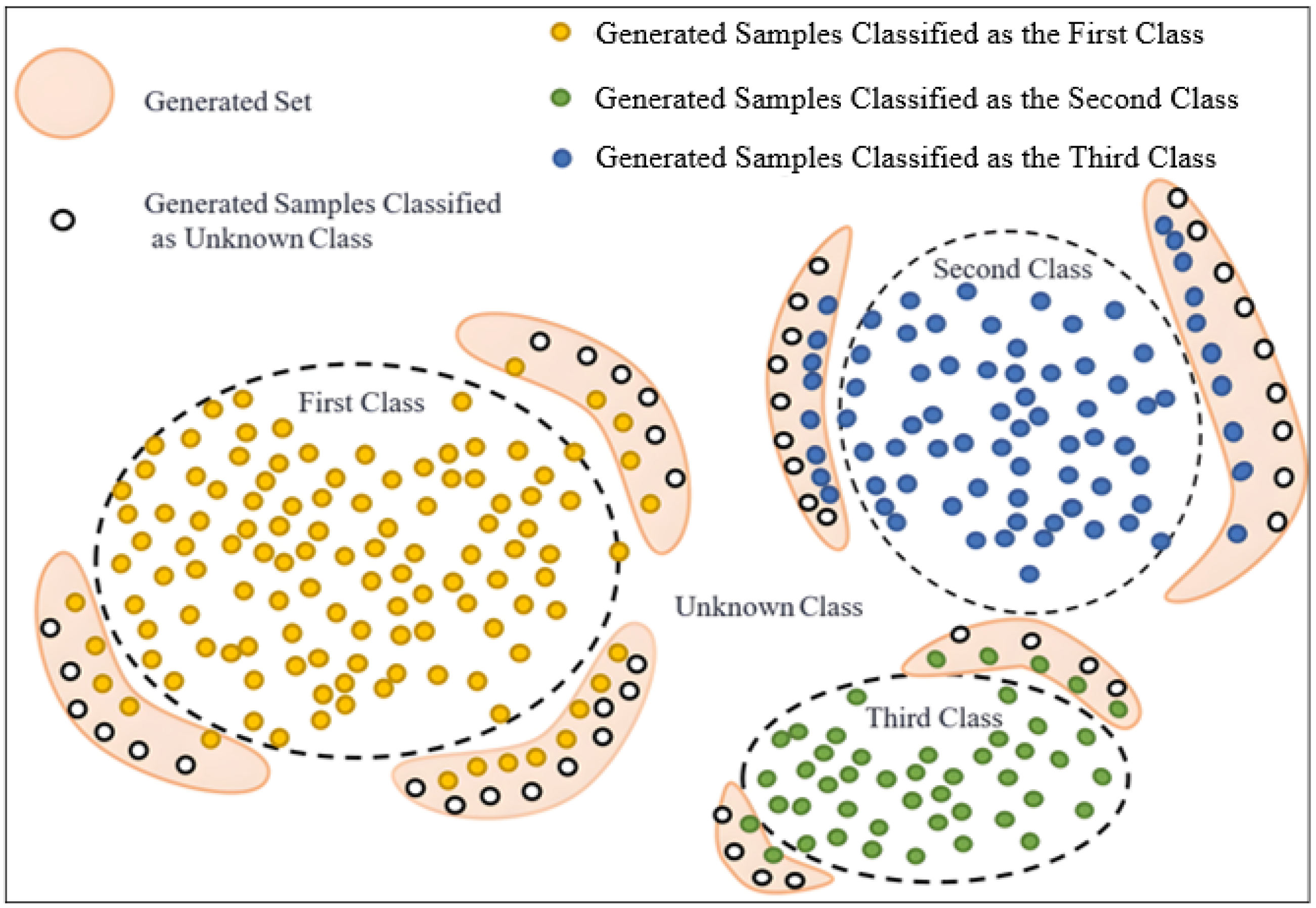
To tackle the aforementioned challenges, this research proposes an open-set HSI classification algorithm based on reciprocal point learning (RPL) and data wandering (DW) (RPLDW). Firstly, a K-class classifier suitable for closed-set problems is trained, with its internal encoder used for extracting image classification features to estimate the feature distribution of known classes. Subsequently, these feature distributions are utilized to optimize the classifier and fine-tune its training. Next, synthetic samples near the decision boundary are generated using a GAN with sample density constraints to solve the few-shot problem, as illustrated in Figure 1.

Concurrently, a framework of RPL is introduced to classify the open-set HSI. The risk of open space is reduced by simulating the out-of-category space to increase the distance between known and unknown categories. In addition, a dynamic threshold method based on DW is devised to build a separate space for each category, thereby enhancing the model’s open-set performance. Employing a DW method, the drifting synthetic samples are categorized into known and unknown categories and inputted together with known samples into the classifier for a new round of training. At this stage, both the closed-set classifier and also a (K+1) class classifier suitable for open-set scenarios are trained in this research, sharing parameters of the early network layers. This approach enhances the data reliability and richness by including generated synthetic samples, ultimately improving the performance of the classification algorithm. The primary contributions of this research can be summarized as follows:

(1)

A method that generates boundaries is proposed based on sample density constraints to calculate sample density. Leveraging information entropy, this approach confines generated samples outside the edge regions of known classes, ensuring proximity to the known classes. Consequently, the classifier can more accurately demarcate the range of known classes.

(2)

The RPL method is adopted to address the open-set HSI classification challenge. It distinguishes the space of unknown categories by constructing inverse prototypes and enlarging the distance between known and unknown categories, thereby reducing the risk of open space. Meanwhile, it reinforces the boundaries of known categories and utilizes dynamic thresholds to remove unknown categories, avoiding manual determination of thresholds and enhancing the robustness of the algorithm.

(3)

A novel sample distribution analysis method is built to screen out edge samples based on DW, enhancing the sample boundaries and improving the classification accuracy.

(4)

Extensive experiments on three benchmark HSIs demonstrate the outstanding performance of the proposed RPLDW in FSOSR tasks, effectively fulfilling the open-set few-shot recognition. Therefore, in the real-world scenario of open-set HSI, RPLDW proves to be more robust and effective in minimizing open risks.

2. Related Works

2.1. Few-Shot Open-Set Recognition

The FSOSR issue is explored in [18] by creating Gaussian clusters that utilize a limited support set. Despite effectively learning the closed-set distribution, the prototypes in PEELER fail to remove outliers, particularly in rejecting spectrally fine-grained outliers. Another approach [17] implements a thresholding technique that relies on the disparity between original prototypes and queried transformed prototypes to identify outliers. Similarly, current FSOSR methods applied to HSI [28,29] also depend on a comparable threshold to exclude outliers. Nonetheless, determining an optimal threshold that can accurately reject outliers presenting a marginal spectral difference to the known land cover samples remains a significant challenge. Furthermore, utilizing the reciprocal points classification loss [30] results in a less compact known class distribution in FSL, contributing to reduced closed-set accuracy.

2.2. Generative Open-Set Recognition

A sophisticated open-set classifier should understand the nuanced closed-set distribution while navigating the open space effectively. Presently, generative OSR methods often address three aspects independently: (1) outlier rejection based on reconstruction error [31,32,33], (2) pseudo-open-set generation [23,34], and (3) enrichment of the closed-set distribution [35,36]. Predominantly, generative OSR methods employ GAN [37] or autoencoder [38] algorithms, leveraging large-scale training datasets. However, the class conditional auto-encoder (C2AE) [38] is susceptible to selection bias of a known sample from the training set, resulting in low reconstruction error on known samples. Research [37] introduces synthetic features and penalizes the discriminator to encourage outlier rejection. The adversarial samples are not proposed to be always considered outliers but can serve as representatives of known classes. A critical challenge in generative FSOSR is the non-convergence of GAN when working with limited training data [39]. The training strategy employed by [38] appears to offer a potential solution to this challenge.

2.3. Data Generated

Research [40] exclusively generates pseudo-known samples by rapidly adapting to a new domain using optimization-based meta-learning techniques, specifically [41] and Reptile [42]. However, it lacks the capability to produce out-of-distribution data. In contrast, [43] focuses solely on generating synthetic data for few-shot classification, while [44] creates synthetic images by combining two noise vectors with a feature vector through unsupervised meta-learning. Research [45] introduces an anti-collapse regularizer to maintain discriminability and diversity in a few-shot setting. The proposed regularizer minimizes the logarithmic similarity among generated adversarial samples and the logarithmic similarity of unit variance Gaussian noise. Furthermore, the approach of fusing input images with random interpolation coefficients in [46] facilitates the generation of arbitrary landcover classes. Additionally, [47] amplifies singular values associated with age, pose, and skin tone derived from singular value decomposition performed on [48]. Nevertheless, the range of end members in HSI datasets is infinite, leading to intractable singular values.

3. Methodology

3.1. Subsection

Herein, a dataset $D_{tr}={\left\{\left(x^{(i)},y^{(i)}\right)\right\}}_{i=1}^K$ containing K-known classes is given (where $x^{(i)}$ is a set of known classes, with $N_i$ samples in each, and $y^{(i)}$ refers to a set with the same one-hot vectors, representing labels corresponding to the set $x^{(i)}$). Under this given condition, it should correctly classify the K-known classes while recognizing and classifying new classes as the (K + 1) class.

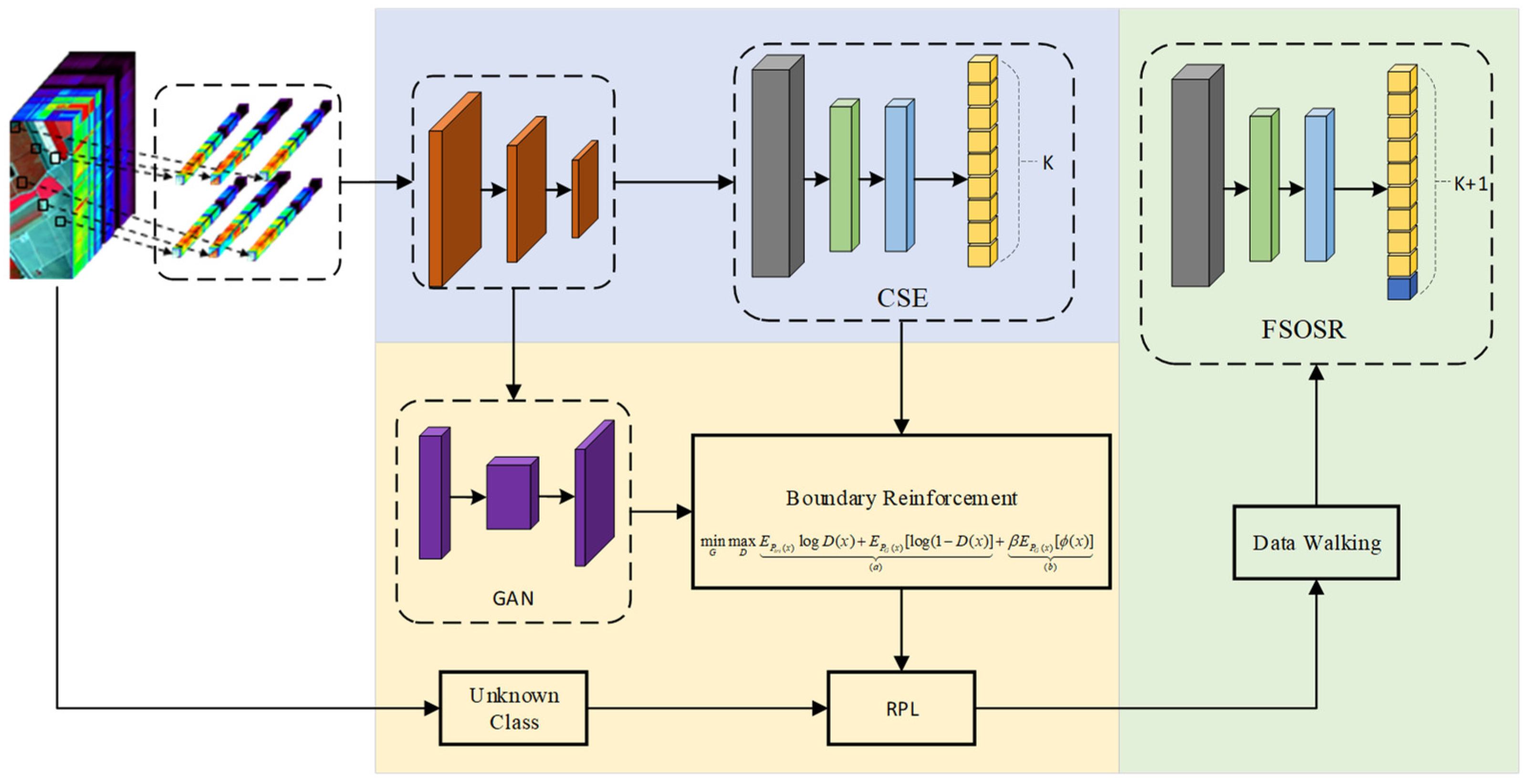
Firstly, a K-class classifier suitable for a closed set is trained in this research, with its encoder being employed to extract image classification features and estimate the feature distribution of all known classes. Meanwhile, the training of the classifier is adjusted based on it. Subsequently, a GAN constrained by sample density is employed to generate synthetic samples near the decision boundaries. Leveraging RPL, this research models the unknown class space to augment the feature distance between the known data after boundary expansion and the unknown data in the open-set space. Then, employing the data walk method, the unclassified synthetic samples are categorized into known and unknown classes and sent to the classifier with the known samples for a new round of training. At this stage, the closed-set classifier and, concurrently, a (K + 1) class classifier suitable for the open set are trained. The training of these two classifiers shares the parameters of the previous layers of the network. The overall network architecture is illustrated in Figure 2.

The multitask network employed in this research requires an input of dimensions 9 × 9 × Channel. The first part of the network is an encoder/feature extractor equipped with two residual units and a global average pooling layer. After extracting latent features, a fully connected layer with a softmax function is set, serving as a classifier to output probabilities to the known classes. The reconstruction task of this research involves gradually increasing the spatial dimension of the latent features through a deconvolution layer. The output of the reconstruction task is a 9 × 9 × Channel instance, w intended to closely resemble the input data by minimizing the loss. Extreme value theory (EVT) is adopted to model the reconstruction loss, thus separating known and unknown classes.

The overall algorithm is outlined in Algorithm 1 below. $W_f$ refers to the synthetics generated by a GAN constrained by sample density, which is composed of $W_{fC}$ and $W_{fO}$ based on DW: $W_{fC}$ is categorized as known classes as edge samples to reinforce the sample boundaries, thus improving the performance of the closed-set classification while $W_{fO}$ simulates the unknown classes and serves as the $\left(K+1\right)$ class to train the open-set classifier $f_{OS}\left(\cdot \right)$.

Algorithm 1 Open-set recognition algorithm for generating decision boundaries based on sample density
Input:
	$D_{tr}={\left\{\left(x^{\left(i\right)},y^{\left(i\right)}\right)\right\}}_{i=1}^K$: Dataset of known classes
	$\theta$: Partition Threshold
	$\alpha$: Density Representative Parameter
Output:
	$f_{OS}\left(\cdot \right)$: Open-Set Classifier
1:	Calculate the sample distribution to establish an information entropy field
2:	GAN generates decision boundary samples based on sample information entropy constraints.
3:	translates to “Train closed set classifier $f_{CS}\left(\cdot \right)$
4:	RPL
5:	FOR  $x^{\left(i\right)}\in D$  DO
6:		Calculate the score of the newly generated fake samples.
7:		Divide $W_{fc}$ into $W_{fc}$ and $W_{fo}$
8:	END FOR
9:	On the basis of $f_{CS}\left(\cdot \right)$, train the open-set classifier $f_{OS}\left(\cdot \right)$ with newly generated samples.

3.2. Generation of Known Class Sample Boundaries Based on Sample Density

This first step is to train a closed-set classifier through metric learning. Subsequently, the values in the pre-logit layer of the classifier are taken as sample points, and all sample points are collected as the sample space to calculate the sample density at any position in the sample feature space based on sample features. Next, the distribution of known classes is analyzed, and the objective function of GAN is constrained to facilitate the generation of samples within the boundary area of known classes and their periphery. In this way, it strengthens the boundary of known samples while increasing the reality and richness of simulated unknown class samples. This section details how to constrain GAN to generate sample boundaries, which is realized by calculating the sample density and training the classifier and GAN.

3.2.1. Training of the Closed-Set Classifier

In this research, a closed-set classifier is trained firstly through metric learning, with the following loss function:

$$L_1=E_{D_{tr}(x,y)}\log \frac{{\displaystyle \sum _{y^m\ne y^n}\exp (-{‖w^{(m)}-w^{(n)}‖}_2^2/T)}}{{\displaystyle \sum _{y^m=y^n}\exp (-{‖w^{(m)}-w^{(n)}‖}_2^2/T)}}+E_{x,y~p_{tri}(x,y)}[\log p_C(y|x)]$$

(1)

where

$$T=\frac{1}{N_{total}}{\displaystyle \sum _{m,n=1}^{N_{total}}{‖w^{(m)}-w^{(n)}‖}_2^2}$$

(2)

This facilitates the classifier in accurate classification while gathering samples with the same label as much as possible, resulting in distinct classes in the sample space as separate clusters. Following this, the parameters of the feature extractor in the classifier are frozen, the distance between each sample point and the center sample is computed, and the classifier is trained.

$$\begin{array}{c}{L}_1=E_{D_{tr}(x,y)}\log \frac{{\displaystyle \sum _{y^m\ne y^n}\exp (-{‖w^{(m)}-w^{(n)}‖}_2^2/T_j)}}{{\displaystyle \sum _{y^m=y^n}\exp (-{‖w^{(m)}-w^{(n)}‖}_2^2/T_j)}}+\lambda E_{x,y~p_{tri}(x,y)}[\log p_C(y|x)]\\ +(1-\lambda )E_{x,y~p_{tri}(x,y)}[r(y|x)]+\beta E_{P_{tri}(x)}[\varphi (x)]\end{array}$$

(3)

where $\lambda ,\beta >0$ is a balancing parameter. Sample points that are close to the center sample have a high-density score. The classifier’s score and the sample density score are bundled together. When the sample is at the sample boundary or floating outside the cluster, the sample density is low, the classifier score is low, and the corresponding predicted label information entropy value is large, increasing the difficulty of being classified into a known class. With such a classifier, training a GAN to generate boundary samples becomes feasible, further refining the constraints on the classifier’s ability to recognize the boundaries of known class samples.

3.2.2. Calculation of Sample Density

There are two challenges when calculating the sample density. Firstly, due to the different aggregation degrees in each cluster, some clusters exhibit a relatively dense distribution of central feature points, while others have spare edges. Consequently, the density estimation of different regions needs to consider the relative positions of distinct clusters. Secondly, a small cluster of sample points is found to be gathered, forming a pseudo-sample center, as described in Figure 3.

The density peak clustering algorithm (DPC) is employed to calculate the maximum diameter ${\mathrm{d}}_{\max }$ of the entire sample space. $\alpha$ points are selected on average contained in each neighborhood, and $\frac{d_{\max } \times \alpha }{{\displaystyle \sum _{i=1}^K{N}_i}}$ serves as the neighborhood radius of a sample point $x_j$. Meanwhile, the number of sample points neighboring the point is counted as the local density ${\rho }_j$ of the point. Finally, the entropy of the region is calculated using the following equation:

$$H_j=\frac{{\displaystyle \sum _{l=1}^{{\rho }_j}{{\mathrm{h}}_{{\rho }_j}}^l}{{\mathrm{lnh}}_{{\rho }_j}}^l}{{\rho }_j}$$

(4)

where

$${h_{{\rho }_j}}^l=\frac{x_l}{{\displaystyle \sum _{j=1}^{{\rho }_j}{x}_j}}$$

(5)

Each data point ${\rho }_j$ can be sorted in ascending order, and the minimum distance ${\delta }_j$ between this sample point and other points with higher density is calculated. The density peak score for this point is calculated as:

$${\gamma }_j=\frac{{\rho }_j\times {\delta }_j}{H_j}$$

(6)

Afterward, the top K points with the highest scores are selected as the center samples of the known class. The distance $R_{tr}={\left\{r^{(i)}\right\}}_{i=1}^K$ between each sample point and the center sample of its class is calculated. Meanwhile, the maximum radius $r_{\max }^{(i)}$ in the i-th class is selected and $\frac{r_{\max }^{(i)}\times \alpha }{N_i}$ refers to the neighborhood radius of each sample point. After that, the number of sample points $N_j$ contained in the neighborhood of the j-th sample is calculated. The aggregation score of the neighborhood where each point is located is calculated as follows:

$${\theta }_j=\frac{N_j\times N_i}{r_{\max }^{(i)}\times \alpha }$$

(7)

Subsequently, the distribution of the known class is estimated through Gaussian kernel density. All sample points are assigned a Gaussian function ${\phi }_j(x)$ with a mean of itself and a variance of ${\theta }_j$. The sum of the Gaussian functions of all sample points forms the energy field, which can be expressed as follows:

$$\varphi (x)={\displaystyle \sum _{j=1}^{N_{tatal}}{\phi }_j(x)}$$

(8)

In the above equation, $N_{\mathrm{total}}$ signifies the number of all sample points in the sample space, based on which the density representation of each position within the sample space can be acquired.

3.2.3. Training of GAN

GAN, typically used to generate pixel images that are as similar as possible to the original images, primarily encompasses discriminators (D) and generators (G). The generator maps the latent variables z to the output space through the prior distribution $P_{\mathrm{pre}}(z)$ and outputs $G(z)$. The discriminator $D(x)\to [0,1]$ represents the probability that the sample comes from the real target distribution. Through the showdown between the generator and the discriminator, the distribution $P_G(x)$ of the samples generated by the generator gradually approaches the target distribution $P_{tri}(x)$. Its objective function is described as follows:

$$\underset{G}{\min } \underset{D}{\max }{E}_{P_{tri}(x)}[\log D(x)]+E_{P_{pre}(z)}[\log (1-D(x))]$$

(9)

This research aims to produce samples on the periphery of the known classes for the generator. For this purpose, the original GAN objective function is modified accordingly, as given in Equation (10) below.

$$\underset{G}{\min } \underset{D}{\max }\underset{(a)}{\underbrace{E_{P_{tri}(x)}\log D(x)+E_{P_G(x)}[\log (1-D(x)]}}+\underset{(b)}{\underbrace{\beta E_{P_G(x)}[\varphi (x)]}}$$

(10)

In the above expression, $\beta >0$ is the balance parameter, which means that the trained classifier becomes a class one at $\beta =0$. This objective function can be delineated into two components. The first term (a) corresponds to the loss of the original GAN, making the samples generated by the generator as similar as possible to the real samples. The second term (b) calculates the sample density. Throughout the training, the generator and the discriminator undergo multiple training iterations under the constraint of sample density. This iterative process eventually guides the generator in producing samples on the low-density boundary and discrete samples.

Equation (10) emphasizes generating authentic images to augment the closed-set training data. To ensure that the generated and the real images are ultimately projected into the same feature space, the conditional generative network should be trained on the basis of the well-trained autoencoder. However, this research deviates from relying on autoencoder training and instead opts to generate synthetic samples by referencing the latent feature layer of the known class. The $W$ chosen refers to the feature value corresponding to the pre-logit layer of the closed-set classifier. The final equation is as follows:

$$\underset{G}{\min } \underset{D}{\max }\underset{(a)}{\underbrace{E_{P_{tri}(w)}\log D(\mathrm{w})+E_{P_G(w)}[\log (1-D(w)]}}+\underset{(b)}{\underbrace{\beta E_{P_G(w)}[\varphi (w)]}}$$

(11)

This approach enables the generator to produce synthetic samples in areas with low sample density, effectively balancing the distribution of internal samples within the known classes and consequently enhancing the accuracy of the classifier. Additionally, generating samples in the low-density regions outside the known classes can train the classifier to recognize unknown class samples by categorizing them as unknown classes. This process provides negative feedback, allowing the model to perceive the boundary area of the known classes.

3.3. Reciprocal Point Learning

Reciprocal points [30] represent the inverse prototypes of each known category, and their utilization enables the constraints of the space outside the category while maintaining the accuracy of the known category. During the training, RPL [49], based on reciprocal points, pushes all known categories towards the edge of the space. As a result, this strategy ensures that the unknown category and reciprocal points collectively define the space outside the category, minimizing the overlap between known and unknown distributions. Consequently, this enhances the distinguishability of the unknown category. In this research, RPL is adopted to model the space of unknown categories to classify the open-set HSI.

Specifically, given there are n labeled samples and N known categories in the training dataset $D_S=\left\{q_1,q_2,\cdots ,q_n\right\}$, $y_i\in \left\{1,2,\cdots ,N\right\}$ is the corresponding label of $q_i$. For trail data $D_T=\left\{t_1,t_2,\cdots ,t_m\right\}$, the labels of $t_i$ belong to $\left\{1,2,\cdots ,N\right\}$ for closed-set HSI classification and to $\left\{1,2,\cdots ,N\right\}\cup \left\{N+1,N+1,\cdots ,N+U\right\}$ for open-set HSI classification, where U denotes the number of unknown categories in a realistic HSI scenario. Thus, the potential unknown data can be denoted as $D_U$. For each known category $k(1\le k\le N)$, $S_k$ is the embedding space in the space $R^D$, and the corresponding open space $O_k$ can be denoted as $O_k=R-S_k$.

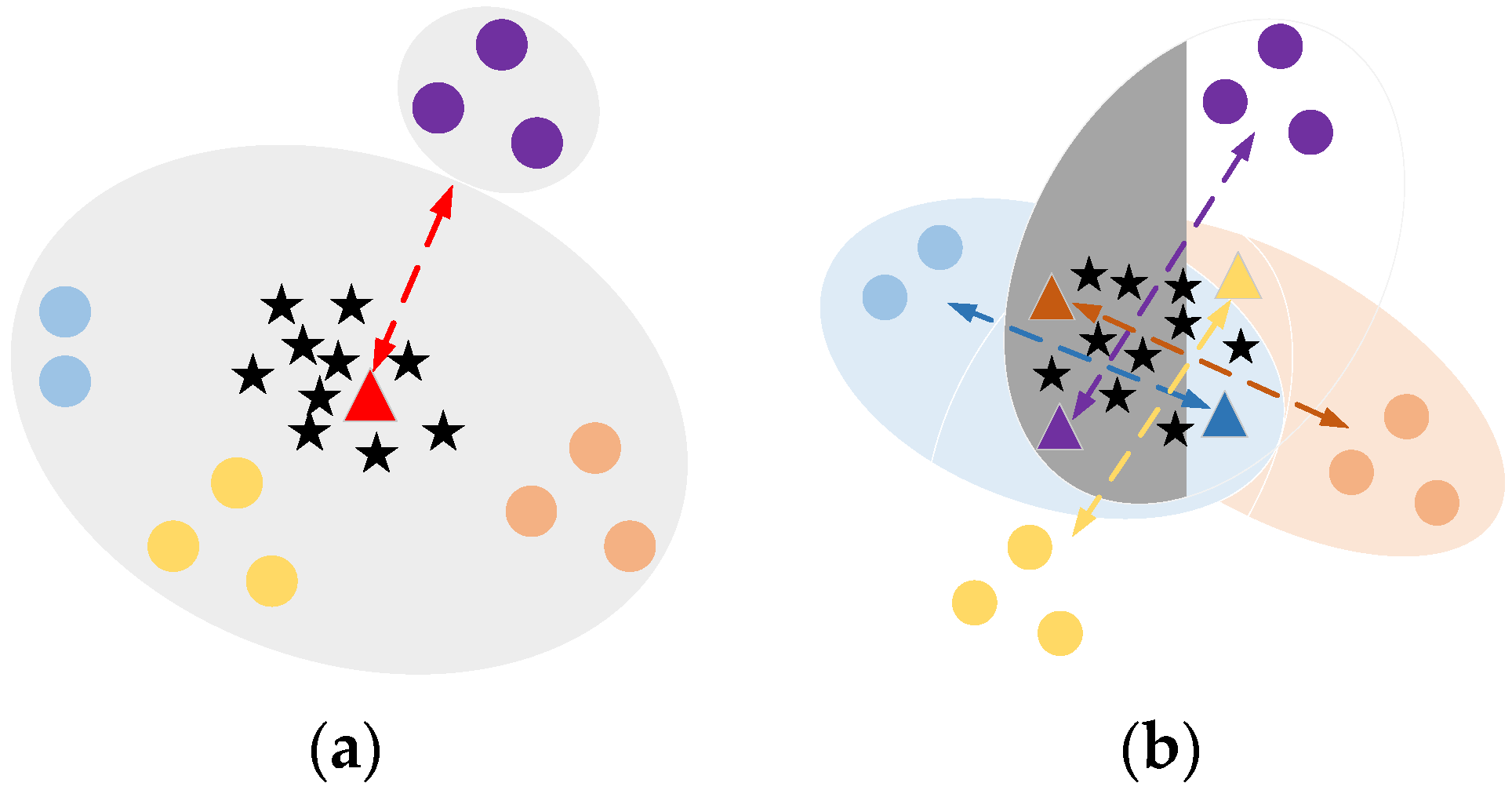
Therefore, as an inverse prototype of the known category $k$, the reciprocal point $P^k$ can be regarded as a potential representation of the sub-dataset $D_L^{\ne k}\cup D_U$ [14]. As demonstrated in Figure 4a, the reciprocal point $P^k$ should be closer to the empty space $O_k$ and far away from $S_k$, as follows.

$$\max (\zeta (D_L^{\ne k}\cup D_U),P^k)\le d\forall d\in \zeta (D_S^k,P^k)$$

(12)

where $\zeta$ denotes a set of distances such that the known category $k$ is maximally distant from $P$.

Therefore, a pivotal objective of RPL is to expand the distance between known categories and their corresponding reciprocal points. To achieve this, the cosine distance $d$ is employed to compute the spatial position and angular orientation between instance $q_i$ and the corresponding reciprocal point $P^k$.

$$d(\phi (q_i),P^k)=1-\frac{\phi (q_i)\cdot P^k}{‖\phi (q_i)‖\cdot ‖P^k‖}$$

(13)

where $\phi (\cdot )$ denotes a feature representation network with a learnable parameter set $\Theta$, and $\phi (q_i)$ refers to a network feature of sample $q_i$.

After describing the distance metric, it is noteworthy that as the distance $d(\phi (x_i),P^k)$ increases, the probability of labeling $q_i$ is calculated as the category $k$. The category probability can be calculated using the softmax function, considering the nature of the reciprocal points and the instance-related weights in the expression below.

$$p(y=k\left|q_i,\phi ,P\right.)=\frac{\exp (d(\phi (q_i),P^k)/{\xi }_i)}{{\displaystyle \sum _{j=1}^N\exp (d(\phi (q_i),P^k)/{\xi }_i)}}$$

(14)

Therefore, the supervised loss function can be defined as the negative logistic loss of the labels:

$$L_C(q,P)=-{\log }_2(1+\exp (-qP))$$

(15)

The learnable parameter set of the feature representation network $\phi (\cdot )$ is updated by minimizing $L_C$. Therefore, $\phi (\cdot )$ can classify the known categories through supervised learning with multi-class samples and their corresponding true labels. More importantly, as illustrated in Figure 4b, all known categories are pushed to the periphery of the space by their respective reciprocal points throughout the training. In addition, reciprocal points in the space outside the category are also pushed into the known space.

3.4. Sample Distribution Using Data Wandering

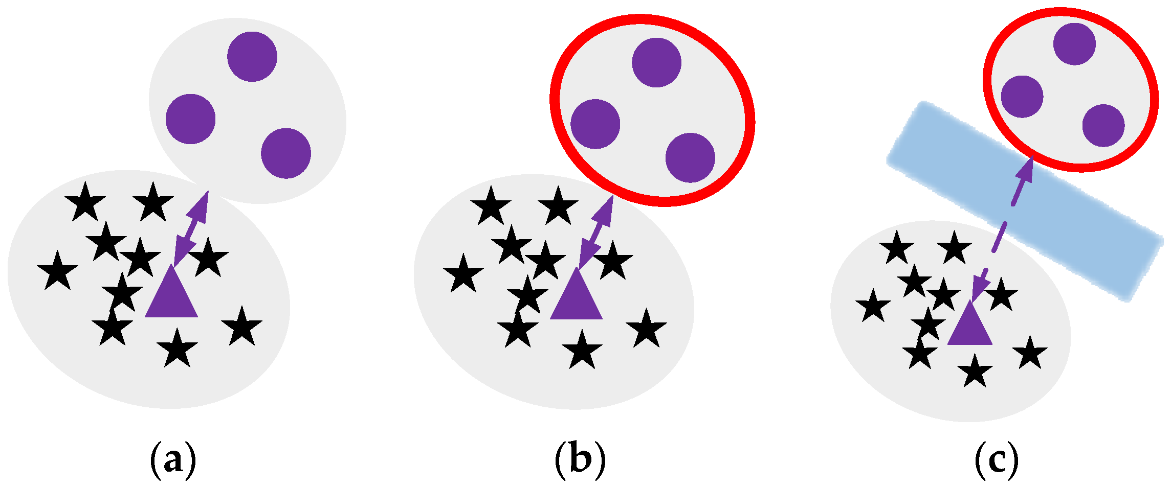
Since the potential unknown categories are in the space outside the categories, the risk of encountering open space persists. In response, a learnable dynamic threshold strategy is further proposed in this research. By constructing a separation space, the open-set HSI classification approach is optimized to lower the risk of the open space and facilitate the recognition of unknown categories. Different from the past approaches that relied on multi-class classifier prediction results for in-class splitting, DW is introduced for sample distribution analysis and further constrains the open space, as explicated in Figure 5.

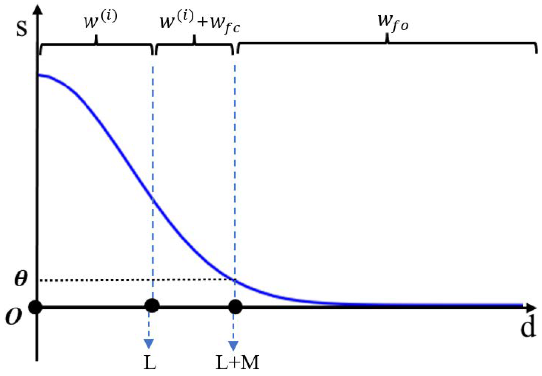
By constructing an information energy field and setting a threshold $\theta$, the sample space is divided into within-class and outside-class after incorporating the synthetic samples. The basic concept is depicted in Figure 6.

In the figure above, the horizontal axis $\mathrm{d}$ represents the distance from the sample to the relative sample center, while the vertical axis $s$ shows the magnitude of the energy value. The interval $\left(0,L\right)$ refers to the central sample $x^{(i)}$ of the known class, the interval $\left(L,L+M\right)$ contains the known class edge samples and some generated samples ($w^{(i)}+w_{fC}$), and the interval $\left(L+M,\infty \right)$ is composed of generated samples $w_{fO}$ only. Existing methods can be employed to directly classify the interval $\left(L,\infty \right)$ as an unknown class, so samples from the known class that are close to the edge are classified as unknown. In this research, some generated samples from the known class are selected to enhance the accuracy of recognition.

Although RPL can classify synthetic samples in the open-set space into unknown class $W_{fO}$ and known class $W_{fC}$. Due to the existence of fuzzy sample boundaries, the boundary samples are categorized as comprehensively as possible, and a data walking method is adopted to iterate. Each sample point is moved in the direction of high energy at a specific step length. Following this, a new data distribution is formed, and the energy field is recalculated. These steps are iteratively repeated several times. After multiple iterations, based on the data redistribution in the open-set space, synthetic samples within the known range are identified as boundary samples through RPL, while the remaining samples are considered new classes.

The data wandering algorithm, as an optimization technique based on energy fields, demonstrates its unique value and efficiency. According to the hypothesis proposed by the decision algorithm, clustering clusters should be centered around high-density data, with low-density data surrounding the high-density ones. In the information energy field, a cluster’s region should exhibit a distribution state where the central energy field strength is high, and the edge energy field strength is low. This paper utilizes $d(\phi (q_i),P^k)$ to construct the information energy field. After forming the sample information energy field values, it is assumed that each sample point can move in the numerical space. By comparing the energy field strength of the sample point with its surrounding eight neighborhoods, the sample point is made to wander toward the direction of higher field strength. After several wanderings, all sample points will move towards regions of higher data energy at a certain step length, forming the final data distribution shape, and the final clustering results are obtained by dividing the regions. Calculating the average energy of samples and setting a threshold can be defined: if the average energy of a clustering cluster is higher than 1.5 times the total average entropy, it is defined as a high-energy cluster; otherwise, it is a low-energy cluster. After the data wandering, due to the energy distribution deviation, i.e., the average energy of the high-energy cluster is far higher than that of the low-energy cluster, new samples in the process of data wandering will tend to move towards high-energy fields. This will result in the following: (1) Data wandering can effectively solve the clustering affiliation of discrete points, making it easier to form clustering clusters after data wandering. (2) In the process of data wandering, high-energy clustering clusters will influence low-energy clustering clusters, causing the clustering results of low-energy clusters to become more dispersed.

Therefore, the RPL constraints for the separation space based on DW can be represented as follows:

$$\begin{array}{l}\max (\theta (D_L^{\ne k}\cup D_U\cup D_{L\to U}^{\ne k}),P^k)\le R,\forall R\in \theta (D_S^k,P^k)\\ \theta =\frac{{\displaystyle \sum \varphi (W_{fO})}}{{\displaystyle \sum \varphi (W_{fC})}}•\log (\frac{{\displaystyle \sum \varphi (W_{fO})}}{{\displaystyle \sum \varphi (W_{fC})}})\end{array}$$

(16)

The process of the data walking method is illustrated in Figure 7 and Figure 8.

4. Experimental Results and Corresponding Analysis

4.1. Dataset

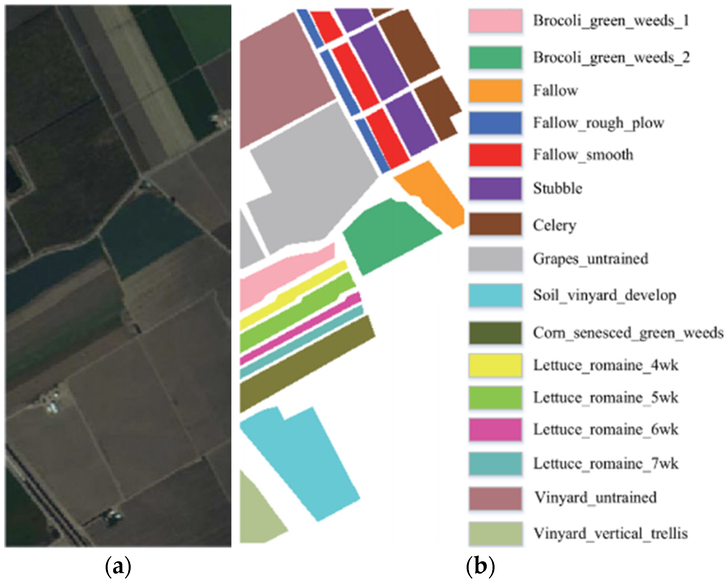
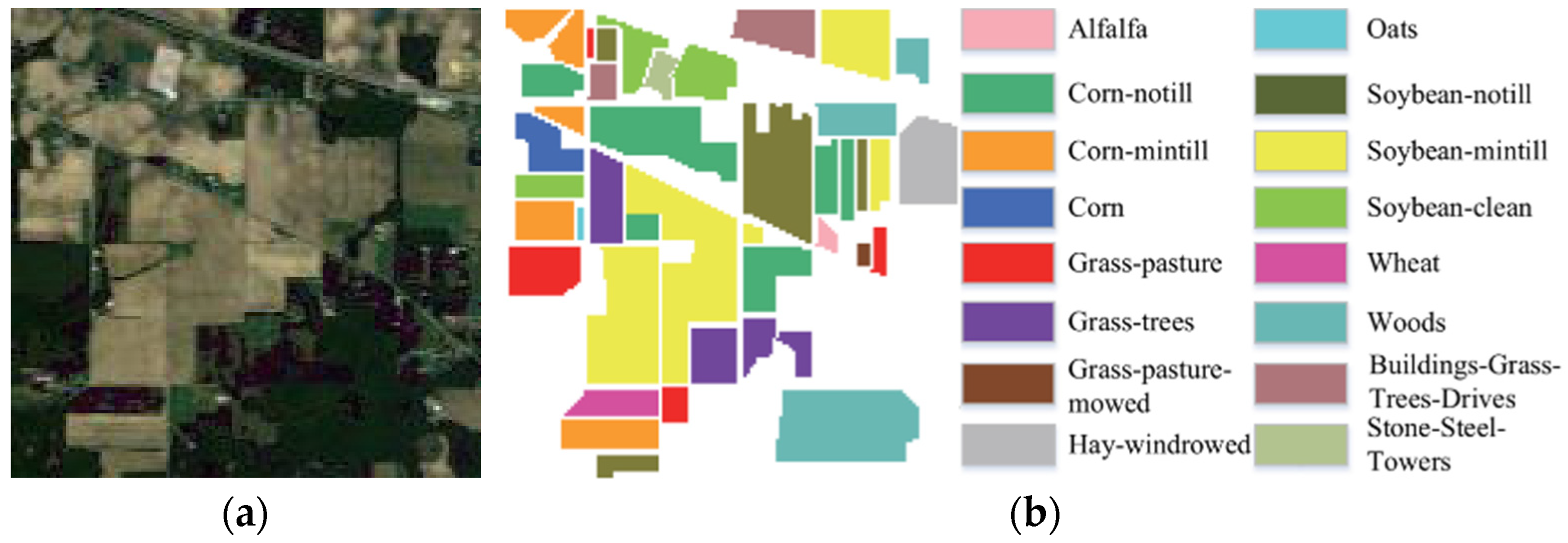
To carry out the open-set HSI multiclassification experiments proposed and to thoroughly validate our methodology, three HSI datasets, Pavia University (PU), Salinas (SA), and Indian Pines (IP) are selected in this research.

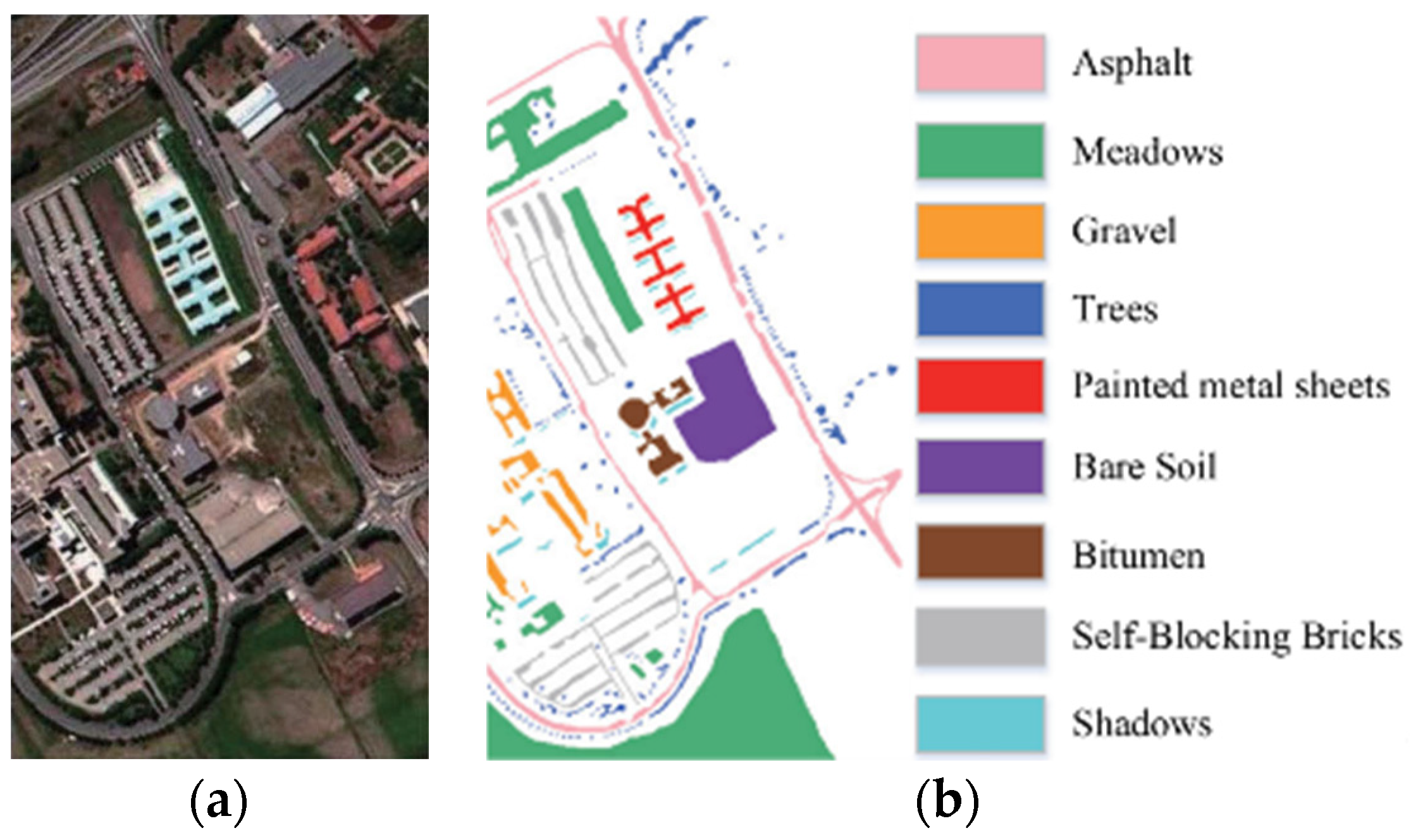
The PU dataset, captured by the reflective optical system imaging spectrometer (ROSIS) near the university, exhibits spatial dimensions of 610 × 340 with a spatial resolution of 1.3 m. It consists of 115 channels covering a wavelength range of 0.43~0.86 μm. Before classification experiments, 12 bands affected by noise and water absorption are eliminated first. Buildings without previous labels are annotated as unknown due to their distinct spectral profiles from known land cover.

The SA dataset is acquired by the Airborne Visible/Infrared Imaging Spectrometer (AVIRIS) over the Salinas Valley in California, USA. The image possesses spatial dimensions of 512 × 217 with a spatial resolution of 3.7 m, and it includes 224 bands spanning a wavelength range of 0.4~2.5 μm. Similarly, 20 bands are removed prior to experiments due to water absorption. Man-made materials without previous annotations are labeled as unknown samples.

The IP dataset, obtained via AVIRIS at the Indian Pines test site in Tippecanoe County, Northwest Indiana, USA, has spatial dimensions of 145 × 145 with a spatial resolution of 20 m. It comprises 220 bands spanning a wavelength range of 0.43~0.86 μm. Before classification experiments, 20 bands are eliminated due to water absorption. Classes with fewer than 10 instances were discarded as tail classes and considered unknown, resulting in 8 known classes. Roads that are not previously labeled are identified as unknown.

Table 1. Statistics of the three HSI databases.

PU			SA			IP
Index	Class Name	Samples	Index	Class Name	Samples	Index	Class Name	Samples
1	Asphalt	6631	1	Brocoli-green-weeds-1	2009	1	Alfalfa	46
2	Meadows	18,649	2	Brocoli-green-weeds-2	3726	2	Corn-notill	1428
3	Gravel	2099	3	Fallow	1976	3	Corn-mintill	830
4	Trees	3064	4	Fallow-rough-plow	1394	4	Corn	237
5	Painted-metal-sheet	1325	5	Fallow-smooth	2678	5	Grass-pasture	483
6	Bare-soil	5029	6	Stubble	3959	6	Grass-trees	730
7	Bitumen	1330	7	Celery	3579	7	Grass-pasture-mowed	28
8	Self-blocking-brick	3682	8	Grapes-untrained	11,271	8	Hay-windrowed	478
9	Shadows	947	9	Soil-vineyard-develop	6203	9	Oats	20
			10	Corn-senesced-green-weeds	3278	10	Soybean-notill	972
			11	Lettuce-romaine-4wk	1068	11	Soybean-mintill	2455
			12	Lettuce-romaine-5wk	1927	12	Soybean-clean	593
			13	Lettuce-romaine-6wk	916	13	Wheat	205
			14	Lettuce-romaine-7wk	1070	14	Woods	1265
			15	Vineyard-untrained	7268	15	Buildings-Grass-Trees-Drives	386
			16	Vineyard-vertical-trellis	1807	16	Stone-Steel-Towers	93

and

Table 2. Physical parameters of the three HSI databases.

	PU	SA	IP
Number of channels	115	224	102
Spectral ranges (μm)	0.43~0.86	0.4~2.5	0.4~2.5
Spatial resolution	610 × 340	512 × 217	1096 × 1096

provides the class distribution for each dataset, while Figure 9a, Figure 10a and Figure 11a are their false color images. Figure 9b, Figure 10b and Figure 11b display the standard true values of the closed-set constant index classification, along with the respective class representations denoted by the true values.

4.2. Evaluation Metrics

To evaluate the performance of RPLDW, the standard OSR indicators are adopted herein, namely closed-set overall accuracy (ClosedOA), open-set overall accuracy (OpenOA), and Kappa. ClosedOA and OpenOA represent the percentage of known category samples and that of open-set samples that are correctly classified, respectively.

$$OpenOA=\frac{{\displaystyle \sum _{k=1}^{K+1}T{P}_k+T{N}_k}}{{\displaystyle \sum _{k=1}^{K+1}T{P}_k+T{N}_k+F{P}_k+F{N}_k}}$$

(17)

where $T{P}_k$, $T{N}_k$, $F{P}_k$, and $F{N}_k$ signify the true positive, true negative, false positive, and false negative of the $k$th known class, respectively. All the outliers are combinedly considered as the ($K+1$)th class in OpenOA.

4.3. Experiments

The ADAM (Adaptive Moment Estimation) optimizer is utilized for back-propagation, with a maximum training round of 100 times. The learning rate is set at 0.0001 for 1-shot and 0.003 for 5-shot. During the training, all experiments are composed in a random manner from the training samples and repeated 10 times to reduce experimental errors. Subsequently, the average results are calculated for analysis and comparison.

To simulate the conditions for open-set HSI classification, the last category of features is designated as unknown, based on generally accepted standard true values of features, to ensure experiment fairness. In addition, setting a single unknown category aids in maintaining the overall effectiveness of the open-set classification image and facilitates in-depth analysis.

To fully assess the performance of our method in open-set HSI classification, several important comparison methods are employed in this work, involving two categories:

(1)

Comparison with traditional closed-set HSI classification methods: the three-dimensional octave convolutional space-spectral attention networks (3DOC-SSAN) [50] and the spectral–spatial transformer network (SSTN) based on transformer backbone [51] are adopted to emphasize the superiority of open-set classification methods in dealing with unknown categories. In this research, a fully connected (FC) layer is introduced at the end of the network for score prediction, where the maximum score serves as the final label. According to the general solution for open-set issues [52], an extra softmax function is added to these networks, and the maximum probability value in the probability vector functions as the prediction label. Referring to [52], the threshold of the softmax function is set to 0.5 to recognize outputs considered as unknown categories (i.e., when the maximum probability is less than 0.5);

(2)

Comparison with open-set HSI classification methods: OpenMax [22], SSLR, and MDL4OW [29] are originally developed for large-scale OSR by fitting the Weibull distribution in the prototype network, making them suitable for FSOSR. RDOSR [25] performs OSR on HSI datasets in the latent space using a limited number of supervised samples. PEELER [26], SnaTCHer [25], and OCN [53] are developed in the context of FSOSR and can be easily evaluated on HSI datasets.

The above comparisons are conducted by adhering to the optimal settings outlined in each original piece of literature. Consistency in the combinations of randomly selected training samples for each method is maintained across 10 experiments to ensure fairness. Notably, each method’s closed-set and open-set performance is validated by recording the closed-set and open-set metrics, respectively. The experimental results are summarized in

Table 3. The 1-shot accuracy (%) of different methods in IP scenarios. (The 16th category is defined as unknown).

Category	3DOC-SSAN	SSTN	OCN	SnaTCHer	PEELER	RDOSR	OpenMax	MDL4OW	SSLR	RPLDW
1	65.70	90. 21	89.24	81.31	80.69	90.23	75.99	75.15	75.83	89.10
2	60.80	58.08	72.60	78.52	78.06	61.71	66.74	66.35	66.35	78.57
3	68.85	61.08	76.35	79.46	81.75	64.89	67.54	69.48	69.48	78.18
4	54.42	70.05	87.56	84.47	81.58	74.43	71.80	69.34	69.34	85.22
5	58.17	64.24	80.30	79.45	78.59	68.25	67.53	66.80	66.80	82.50
6	59.02	69.47	86.83	87.03	88.73	73.81	73.98	75.42	75.42	85.10
7	61.37	71.28	89.10	79.87	79.56	75.74	67.89	67.63	67.63	86.98
8	63.35	71.20	89.00	88.98	87.43	75.65	75.64	74.31	74.31	87.79
9	68.88	70.21	87.77	89.10	86.88	74.60	75.74	73.85	73.85	84.92
10	52.14	62.96	78.71	72.14	63.15	66.90	61.32	53.68	53.68	77.56
11	45.32	52.91	66.13	61.60	54.63	56.21	52.36	59.49	59.49	74.52
12	45.78	68.01	85.01	79.01	62.20	72.26	67.16	52.87	52.87	83.07
13	70.10	71.03	88.79	88.88	88.88	75.47	75.55	75.55	75.55	86.55
14	54.78	68.59	85.74	85.09	81.35	72.88	72.32	69.15	69.15	83.12
15	67.90	69.25	86.56	81.35	78.94	73.58	69.15	67.10	67.10	84.14
Unknown	66.29	69.81	83.21	86.32	85.48	80.14	73.37	72.66	72.66	88.62
Closed OA	64.47	65.29	81.61	80.82	76.34	69.37	68.70	64.89	64.89	82.30
Closed AA	71.59	66.90	83.62	83.10	77.81	71.08	70.63	66.13	66.13	84.09
Closed Kappa	61.39	63.66	79.57	78.89	74.21	67.63	67.05	63.08	63.08	79.82
Open OA	53.13	59.60	74.50	75.95	74.98	63.33	64.56	63.73	63.73	77.03
Open AA	46.68	60.75	75.93	80.00	75.87	64.54	68.00	64.49	64.49	80.57
Open Kappa	50.44	59.18	73.97	75.60	72.44	62.88	64.26	61.57	61.57	76.36

,

Table 4. The 1-shot accuracy (%) of different methods in SA scenarios. (The 16th category is defined as unknown).

Category	3DOC-SSAN	SSTN	OCN	SnaTCHer	PEELER	RDOSR	OpenMax	MDL4OW	SSLR	RPLDW
1	75.82	78.25	91.82	89.12	89.12	90. 86	76.01	79.32	82.61	89.60
2	65.54	78.37	72.62	78.53	78.08	61.73	66.75	82.33	84.37	88.44
3	61.36	78.37	76.37	79.48	81.77	64.91	67.56	85.27	84.76	89.73
4	61.97	77.57	87.58	84.49	81.60	74.44	71.82	84.53	84.10	88.78
5	62.11	75.84	80.32	79.47	78.61	68.27	67.55	82.56	84.29	88.92
6	78.04	78.11	86.85	87.05	88.75	73.82	73.99	83.36	83.11	85.25
7	77.09	78.14	89.12	79.89	79.58	75.75	77.00	82.39	81.67	86.79
8	57.18	63.57	89.02	89.00	87.45	75.67	75.65	67.27	65.68	78.92
9	69.80	78.29	87.79	89.12	86.90	74.62	75.75	85.21	84.70	88.60
10	66.73	74.83	78.72	72.16	63.17	66.92	61.34	82.54	82.02	85.56
11	58.81	77.66	66.15	61.61	67.64	56.23	52.37	84.05	80.51	88.73
12	56.11	77.94	85.03	79.03	62.21	72.28	67.18	85.45	85.52	89.32
13	74.22	78.18	88.81	88.91	88.91	75.49	75.57	85.12	85.18	88.10
14	57.33	77.59	85.76	85.11	81.37	72.90	72.34	84.89	84.84	86.60
15	41.75	68.73	86.58	81.37	78.96	73.60	69.16	72.06	71.25	80.43
Unknown	41.37	43.81	53.03	62.60	53.43	49.63	55.23	54.09	49.40	56.21
Closed OA	59.85	74.02	81.63	80.84	76.36	69.39	68.71	79.37	83.12	86. 94
Closed AA	63.48	75.69	83.64	83.12	77.82	71.09	70.65	82.94	82.46	88.22
Closed Kappa	57.75	73.49	79.59	78.90	74.23	67.65	75.07	77.55	76.35	85.49
Open OA	53.23	69.91	81.00	82.58	81.52	68.85	70.19	75.60	76.05	82.96
Open AA	53.72	70.81	82.56	86.98	82.49	70.17	73.93	77.26	77.66	83.18
Open Kappa	50.77	69.14	80.42	82.02	78.76	68.36	69.86	74.49	74.98	82.14

,

Table 5. The 1-shot accuracy (%) of different methods in PU scenarios. (The 9th category is defined as unknown).

Category	3DOC-SSAN	SSTN	OCN	SnaTCHer	PEELER	RDOSR	OpenMax	MDL4OW	SSLR	RPLDW
1	47.20	78.69	72.81	56.93	74.76	78.12	74.20	82.23	78.11	77.17
2	58.66	80.05	74.08	59.89	76.04	80.85	78.35	85.10	82.48	82.44
3	48.17	80.09	72.94	50.14	76.09	75.71	75.99	79.70	79.98	79.65
4	77.18	81.82	79.82	76.76	77.73	80.35	79.94	84.58	84.15	78.18
5	81.03	88.10	83.68	82.00	83.70	67.80	79.24	71.37	83.41	87.41
6	65.67	84.46	78.48	52.39	80.24	79.73	78.21	83.93	82.33	84.06
7	73.06	87.34	81.55	61.36	82.97	80.55	79.30	84.79	83.47	84.69
8	49.11	77.55	70.22	50.65	73.68	74.30	67.64	78.21	71.20	72.09
Unknown	45.03	49.28	59.78	53.18	29.91	35.98	43.60	37.88	45.90	62.30
Closed OA	57.75	83.13	83. 17	65. 69	78.98	77.48	78.42	81.56	82.55	85.35
Closed AA	60.23	84.46	80.04	61.93	80.24	78.27	78.92	82.39	83.07	84.79
Closed Kappa	48.81	81.52	77.02	53.38	77.45	77.02	77.24	81.07	81.31	83.63
Open OA	48.93	59.87	73.46	57.93	75.88	73.67	74.67	77.55	78.60	80.28
Open AA	49.68	57.60	68.88	54.63	73.72	73.34	73.50	77.20	77.37	78.67
Open Kappa	50.64	57.43	70.50	51.34	73.56	72.63	72.96	76.45	76.80	77.93

,

Table 6. The 5-shot accuracy (%) of different methods in IP scenarios. (The 16th category is defined as unknown).

Category	3DOC-SSAN	SSTN	OCN	SnaTCHer	PEELER	RDOSR	OpenMax	MDL4OW	SSLR	RPLDW
1	73.00	99. 56	99. 01	99.00	99.00	99.32	84.43	83.50	84.26	99.00
2	67.56	64.54	80.67	87.24	86.73	68.57	74.15	73.72	73.72	87.30
3	76.50	67.86	84.83	88.29	90.83	72.11	75.05	77.21	77.21	86.87
4	60.46	77.83	97.29	93.86	90.64	82.70	79.78	77.04	77.04	94.69
5	64.63	71.38	89.22	88.28	87.32	75.84	75.04	74.22	74.22	91.67
6	65.58	77.18	96.48	96.70	98.59	82.01	82.20	83.80	83.80	94.55
7	68.18	79.20	99.00	88.74	88.40	84.15	75.43	75.14	75.14	96.64
8	70.38	79.11	98.89	98.87	97.14	84.06	84.04	82.57	82.57	97.54
9	76.54	78.02	97.52	99.00	96.53	82.89	84.15	82.05	82.05	94.36
10	57.94	69.96	87.45	80.16	70.17	74.33	68.14	59.64	59.64	86.18
11	50.35	58.78	73.48	68.44	60.70	62.46	58.17	66.10	66.10	82.80
12	50.87	75.57	94.46	87.79	69.11	80.29	74.62	58.74	58.74	92.30
13	77.89	78.92	98.65	98.76	98.76	83.85	83.95	83.95	83.95	96.17
14	60.87	76.22	95.27	94.54	90.39	80.98	80.36	76.83	76.83	92.36
15	75.45	76.94	96.18	90.39	87.71	81.75	76.83	74.55	74.55	93.49
Unknown	73.66	77.57	92.46	95.91	94.98	89.04	81.52	80.73	80.73	98.47
Closed OA	71.63	72.54	90.68	89.80	84.82	77.08	76.33	72.10	72.10	91.44
Closed AA	71.59	74.33	92.91	92.33	86.45	78.97	78.48	73.48	73.48	93.43
Closed Kappa	68.22	70.73	88.41	87.65	82.46	75.15	74.50	70.09	70.09	88.69
Open OA	59.03	66.22	82.78	84.39	83.31	70.36	71.73	70.81	70.81	85.59
Open AA	51.86	67.50	84.37	88.89	84.30	71.71	75.56	71.66	71.66	89.52
Open Kappa	56.04	65.75	82.19	84.00	80.49	69.86	71.40	68.42	68.42	84.84

,

Table 7. The 5-shot accuracy (%) of different methods in SA scenarios. (The 16th category is defined as unknown).

Category	3DOC-SSAN	SSTN	OCN	SnaTCHer	PEELER	RDOSR	OpenMax	MDL4OW	SSLR	RPLDW
1	83.32	85.99	99.01	97.94	97.94	99. 32	83.52	87.16	90.78	98.46
2	72.02	86.12	79.80	86.30	85.80	67.83	73.36	90.48	92.71	97.19
3	67.42	86.12	83.92	87.34	89.85	71.33	74.24	93.71	93.15	98.6
4	68.10	85.24	96.24	92.85	89.67	81.81	78.92	92.89	92.42	97.56
5	68.25	83.35	88.26	87.33	86.38	75.02	74.23	91.66	92.63	97.71
6	85.76	85.83	95.44	95.66	97.53	81.13	81.31	91.60	91.33	93.68
7	84.71	85.87	97.94	87.79	87.45	83.25	84.62	90.54	89.75	95.37
8	62.83	69.86	97.83	97.81	96.10	83.15	83.14	73.92	72.18	86.72
9	76.70	86.03	96.47	97.94	95.49	82.00	83.25	93.64	93.07	97.36
10	73.33	82.23	86.51	79.30	69.42	73.53	67.40	90.71	90.13	94.02
11	64.62	85.34	72.69	67.70	30.37	61.79	57.55	92.36	88.47	97.5
12	61.66	85.65	93.44	86.85	68.37	79.43	73.82	93.90	93.98	98.15
13	81.56	85.91	97.59	97.70	97.70	82.95	83.04	93.54	93.60	96.81
14	63.00	85.26	94.25	93.52	89.42	80.11	79.49	93.29	93.23	95.17
15	45.88	75.52	95.15	89.42	86.77	80.87	76.01	79.19	78.30	88.39
Unknown	45.46	48.14	58.28	68.79	58.71	54.54	60.69	59.44	54.29	61.77
Closed OA	65.77	81.34	89.70	88.83	83.91	76.25	75.51	87.22	91. 91	96. 39
Closed AA	69.76	83.18	91.91	91.34	85.52	78.12	77.64	91.14	90.61	96.94
Closed Kappa	63.47	80.76	87.46	86.71	81.57	74.34	73.70	85.22	83.90	93.94
Open OA	58.50	76.82	89.01	90.74	89.58	75.66	77.13	83.08	83.57	91.16
Open AA	59.04	77.81	90.72	95.58	90.65	77.11	81.24	84.90	85.34	91.41
Open Kappa	55.79	75.98	88.38	90.13	86.55	75.12	76.77	81.85	82.39	90.26

and

Table 8. The 5-shot accuracy (%) of different methods in PU scenarios. (The 9th category is defined as unknown).

Category	3DOC-SSAN	SSTN	OCN	SnaTCHer	PEELER	RDOSR	OpenMax	MDL4OW	SSLR	RPLDW
1	53.03	88.42	81.80	63.96	84.00	87.77	83.37	92.39	87.76	86.71
2	65.91	89.94	83.24	67.29	85.44	90.84	88.04	95.62	92.67	92.63
3	54.12	89.99	81.96	56.34	85.49	85.07	85.38	89.55	89.87	89.49
4	86.72	91.93	89.69	86.25	87.33	90.28	89.82	95.03	94.55	87.84
5	91.05	98.99	94.02	92.13	94.04	76.18	89.03	80.19	93.72	98.21
6	73.79	94.90	88.18	58.86	90.16	89.59	87.88	94.30	92.50	94.45
7	82.09	98.13	91.63	68.94	93.22	90.51	89.10	95.27	93.79	95.16
8	55.18	87.14	78.90	56.91	82.78	83.49	76.00	87.88	80.00	81.00
Unknown	50.59	55.37	67.16	59.75	33.60	40.43	48.99	42.56	51.57	70.00
Closed OA	64.89	93.41	93.94	71. 51	88.74	87.06	88.11	91.64	92.75	95.90
Closed AA	67.67	94.90	89.94	69.59	90.16	87.94	88.67	92.57	93.34	95.27
Closed Kappa	54.84	91.60	86.54	59.97	87.02	86.54	86.79	91.09	91.36	93.97
Open OA	54.98	69.74	82.54	65.09	85.25	82.77	83.89	87.13	88.31	90.20
Open AA	55.82	67.19	77.40	61.38	82.83	82.40	82.58	86.74	86.93	88.39
Open Kappa	56.90	67.00	79.21	57.68	82.65	81.61	81.98	85.90	86.29	87.56

.

4.4. Experimental Results

The RPLDW is compared with the most advanced 1-shot and 5-shot FSOSR methods in Table 2, Table 3, Table 4, Table 5, Table 6, Table 7, respectively. The HSI datasets demonstrate superior performance compared to other OSR methods. The following valuable conclusions can be drawn from the observed results.

(1)

Limitations of Closed-Set Methods and the Impact of Sample Size on Accuracy: While the use of the softmax function at the end of networks enhances the ability of other closed-set methods to recognize unknown categories, these methods exhibit significant fluctuations when confronted with potential unknown categories. This is especially pronounced in the FSOSR context with limited samples. Methods like 3DOC-SSAN and SSTN perform well with ample samples but become unstable with fewer samples, leading to decreased performance in open-set environments. This highlights the inherent limitations of closed-set classifiers in FSOSR contexts.

(2)

Performance Comparison of Open-Set Methods and Traditional Classification Methods: Both traditional classification methods and those designed for open sets generally do not perform as well in open-set environments as they do in closed-set ones. This phenomenon is more evident in the context of FSOSR. Dedicated open-set methods, such as RPLDW, demonstrate greater resilience and stability, especially under limited sample conditions, by considering the capability to process unknown categories during the design phase.

(3)

Correlation Between Open-Set and Closed-Set Performance: Both conventional classification methods and specialized open-set classification methods reveal a close relationship between open-set and closed-set performance. In FSOSR contexts, if a method excels in open-set performance, it often also performs well in closed-set scenarios, but the reverse is not necessarily true.

(4)

Superiority of Open-Set Methods: Open-set methods exhibit stable accuracy in handling both open and closed-set classifications, which is particularly crucial in FSOSR environments. Compared to closed-set methods, specialized open-set methods effectively exclude unknown categories while maintaining high accuracy in recognizing known categories.

(5)

Advantages of the RPLDW Method: In the FSOSR environment, the RPLDW method outperforms all other studied methods. It scores highest in closed and open-set metrics and achieves the highest accuracy in identifying unknown categories. RPLDW enhances the boundaries of known categories, eliminating the need to manually set specific thresholds. It constructs an independent space in limited sample situations and employs RPL to calculate reciprocal point distances. This approach significantly improves accuracy by determining labels within the known range in open-set scenarios.

Therefore, it can be concluded that RPLDW performs more robustly and effectively when dealing with open risks in the real open world.

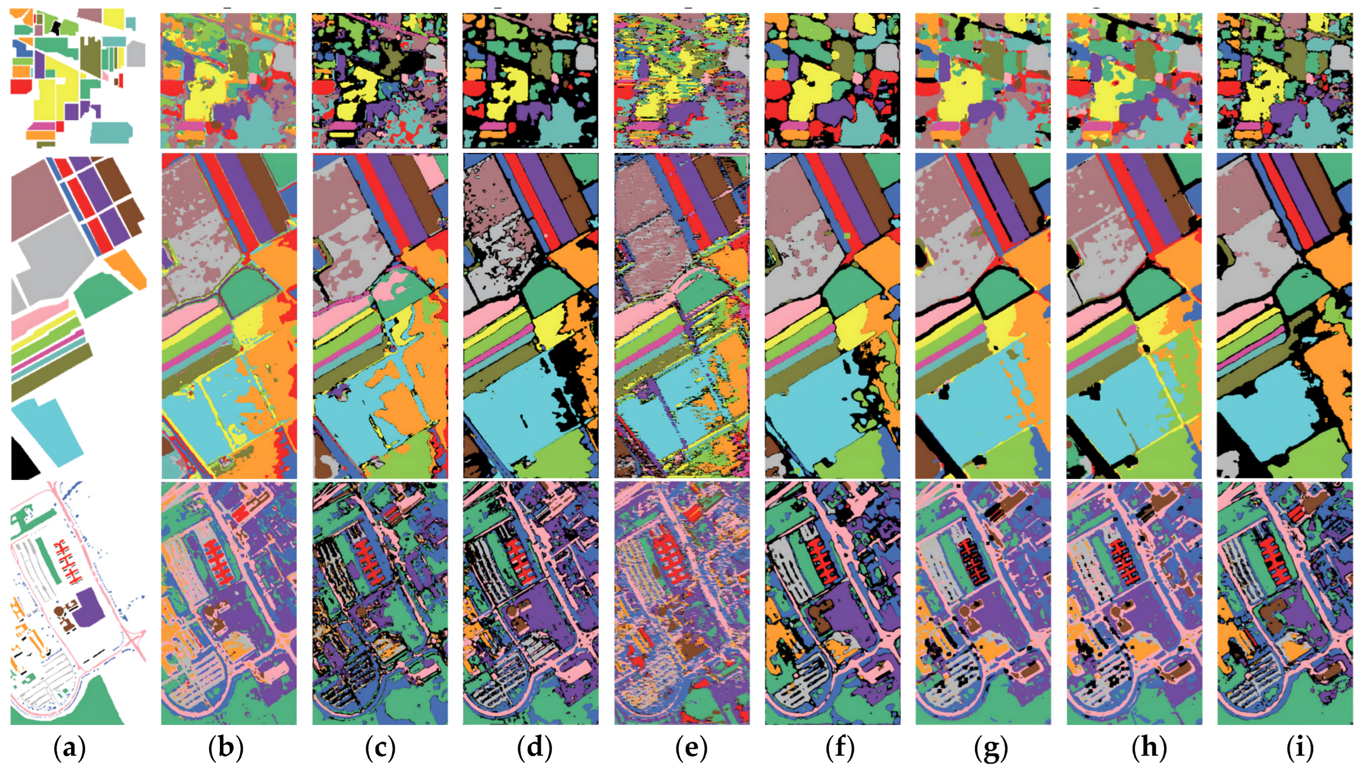
To compare the effects of different methods more intuitively, the classification maps depicting the performance of the better-performing open-set classification methods in the experiment are generated, as explicated in Figure 12. This visual approach provides a better comprehension and comparison of the performance differences among various methods.

Figure 12 reveals that high closure metrics usually align with high-quality closed-set classification maps, whereas low closure metrics may result in subpar outcomes. Despite SSTN demonstrating superior open performance compared to other closed-set methods, it still struggles to effectively exclude unknown categories.

Improved closed-set methods can identify potential unknown categories, as evidenced by the black areas in the open-set classification maps. However, the overall open-set performance of closed-set methods falls short of ideal. The primary issue lies in misclassifying a considerable number of known categories as unknown, causing inconsistencies between the black areas of the open-set classification maps and the actual situation.

The negative impact of the OSE slightly influences the performance of the open-set methods. The classification maps of open-set methods achieve superior visual effects in both the ideal closed-set assumption and the realistic open HSI world. They usually correspond with the actual distribution of ground objects and exhibit less noise.

RPLDW demonstrates excellent visual effects on both closed-set and open-set classification maps, providing further evidence of its robustness and superior performance in the realistic open HSI world. Notably, MDL4OW and SSLR, with fixed thresholds, tend to overlook certain potential areas of unknown categories. In contrast, our proposed RPLDW incorporates a dynamic, learnable threshold, enabling it to discover more potential areas of unknown categories. This adaptive approach proves effective in navigating the complex open world with new ground object categories.

4.5. Open-Set Multiclassification and Visualization Analysis

Herein, categories 11, 12, 13, and 14 of the SA datasets are identified as unknown for open-set multiclassification experimental analysis. The experiments are compared with the latest open-set recognition algorithms, including FCPN [15], DLRSPs-DAEs [54], POSM [15], and SSMLP-RPL [14]. The other detailed settings are consistent with the above-mentioned experiments, and the results are outlined in

Table 9. Multiclassification accuracy of different methods in SA scenarios (%).

Category	FCPN	DLRSPs-DAEs	POSM	SSMLP-RPL	RPLDW
1.00	99.00	99.00	98.46	97.01	98.45
2.00	87.30	87.02	97.19	97.39	98.19
3.00	86.87	88.85	98.60	98.33	98.11
4.00	94.69	92.67	97.56	97.42	97.51
5.00	91.67	89.50	97.71	97.61	97.43
6.00	94.55	96.57	93.68	94.91	95.94
7.00	96.64	92.52	95.37	94.92	97.86
8.00	97.54	97.34	86.72	81.35	89.74
9.00	94.36	95.45	97.36	97.67	98.52
10.00	86.18	78.18	94.02	94.45	96.39
15.00	82.80	86.75	97.50	95.32	91.89
16.00	92.30	80.71	98.15	98.54	98.00
Unknown	78.47	76.73	61.77	74.20	79.32
Closed OA	91.44	88.13	91. 39	92. 63	92.9
Closed AA	93.43	89.94	96.94	96.16	95.98
Closed Kappa	88.69	85.58	93.94	91.13	92.14
Open OA	85.59	84.45	91.16	89.57	93.65
Open AA	89.52	86.91	91.41	90.62	91.57
Open Kappa	84.84	82.67	90.26	88.50	90.34

.

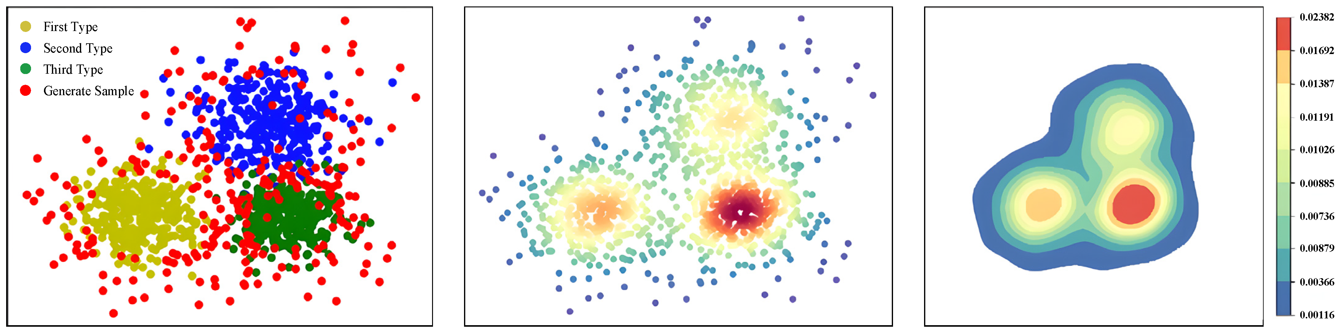
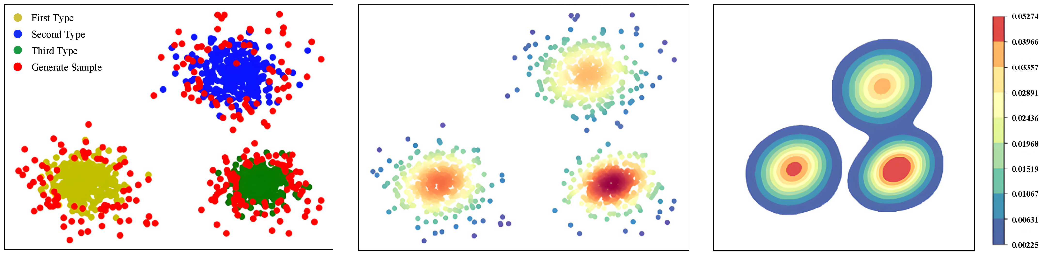
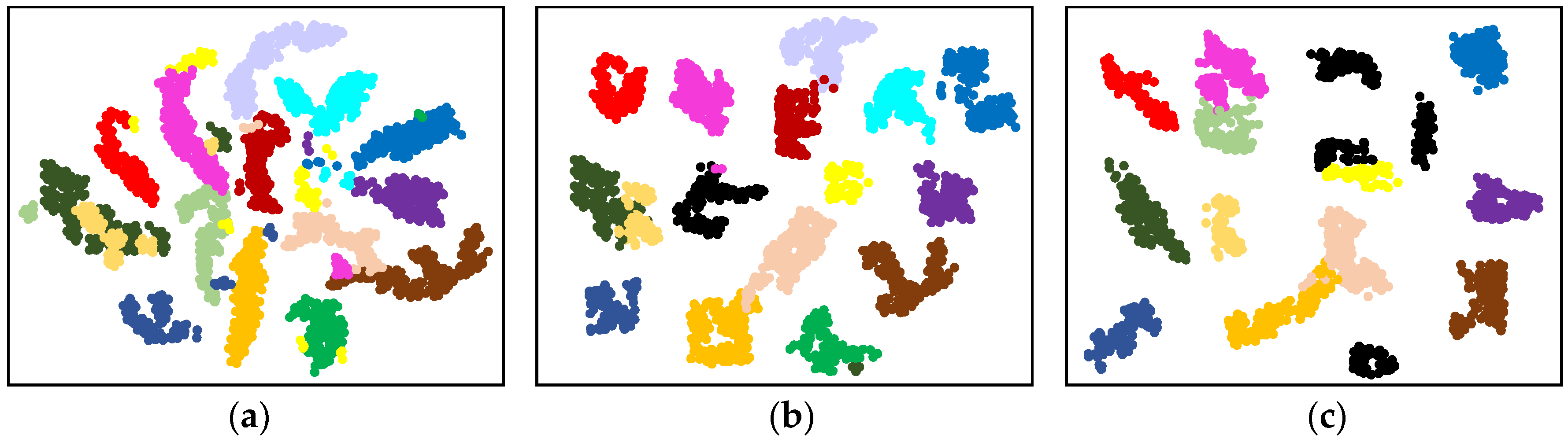
To further intuitively demonstrate the discriminative feature space constructed by RPLDW, the t-SNE dimensionality reduction visualization method is utilized to further highlight its advantages in identifying known and unknown categories. This is implemented by taking SA data as an example, and the results are visualized in Figure 13.

Examining the original SA data reveals suboptimal discriminability in its feature space, primarily presenting as overlap and too much closeness among different categories. However, using the RPL training and DW strategy, the data samples are successfully projected into a more distinctive high-dimensional feature space, enabling the open-set HSI classification. More specifically, the distance between known categories and their corresponding antipodes is broadened, pushing known categories towards the fringe of the space. In addition, the distance between unknown categories and antipodes is confined within a limited boundary. Therefore, the feature space created by RPLDW enhances the distance between known categories and unknown categories, facilitating the identification of unknown categories.

This optimized feature space ensures the correct classification of known categories while effectively excluding unknown categories. More importantly, the label assignment for the instance to be classified is determined by its distance to the antipode. Setting a reasonable threshold can effectively reject unknown categories, thereby mitigating the risk of open space. However, a single and fixed threshold could potentially lead to overlooking potential unknown categories due to variations in the distance between known categories and their antipodes. A learnable dynamic threshold strategy is proposed in this research to address this issue. It can reject unknown categories to the maximum extent without affecting the recognition of known categories.

4.6. Small Sample Analysis

For experiments on HSI data, the samples in each category are randomly disrupted, and the number of samples from each category is set as 20, 50, 150, and 200 labeled with the real class label, forming the training dataset. Importantly, the training dataset does not include samples labeled as “Unknown”. To create the test dataset, the remaining labeled data are combined with the samples labeled as “Unknown”. Furthermore, five repeated tests are conducted following the aforementioned steps to mitigate the potential impact of random factors and ensure the robustness of the experimental outcomes. The algorithm’s performance is assessed using the average classification results. To assess the efficacy of the algorithm proposed in this research, its experimental results are compared with those of several algorithms mentioned in the previous section, employing three experimental datasets. The specific comparisons are detailed in

Table 10. Overall classification accuracy on IP dataset (%).

Sample Size		MDL4OW	SSLR	FCPN	DLRSPs-DAEs	POSM	SSMLP-RPL	RPLDW
20	Unknown	93.05	92.15	96.51	93.70	94.95	94.03	97.48
	Open OA	81.87	80.83	84.41	81.96	83.54	82.48	84.73
	Open AA	86.24	81.79	86.03	83.52	88.00	83.46	88.62
	Open Kappa	81.50	78.09	83.81	81.37	83.16	79.68	83.99
50	Unknown	95.40	94.48	98.95	96.06	97.35	96.41	99.21
	Open OA	83.94	82.87	86.55	84.03	85.65	84.56	88.15
	Open AA	88.42	83.85	88.20	85.63	90.23	85.56	92.20
	Open Kappa	83.56	80.06	85.93	83.42	85.26	81.69	87.39
100	Unknown	97.49	96.81	91.38	98.43	99.48	98.78	99.52
	Open OA	86.01	84.91	88.68	86.10	87.76	86.64	90.72
	Open AA	90.60	85.92	90.37	87.74	92.45	87.67	94.89
	Open Kappa	85.61	82.03	88.04	85.48	87.36	83.71	89.93
150	Unknown	97.55	97.17	93.82	90.80	99.54	99.16	99.82
	Open OA	88.08	86.95	90.81	88.16	89.87	88.72	93.72
	Open AA	92.78	87.98	92.55	89.85	94.67	89.78	98.02
	Open Kappa	87.67	84.00	90.16	87.53	89.46	85.72	92.90
200	Unknown	97.59	97.54	96.26	93.16	99.58	99.53	99.94
	Open OA	90.14	88.99	92.94	90.23	91.98	90.81	94.14
	Open AA	94.95	90.05	94.72	91.96	96.89	91.89	98.47
	Open Kappa	89.73	85.98	92.27	89.59	91.56	87.73	93.33

,

Table 11. Overall classification accuracy on SA dataset (%).

Sample Size		MDL4OW	SSLR	FCPN	DLRSPs-DAEs	POSM	SSMLP-RPL	RPLDW
20	Unknown	60.06	55.23	61.26	60.64	60.68	56.15	61.15
	Open OA	84.84	85.35	90.04	87.42	86.57	87.09	90.25
	Open AA	86.70	87.16	91.20	88.54	88.47	88.93	90.49
	Open Kappa	83.59	84.15	89.05	86.45	85.30	85.87	89.36
50	Unknown	60.97	56.60	61.90	61.27	61.61	57.55	63.62
	Open OA	87.41	87.94	92.77	90.06	89.20	89.73	93.89
	Open AA	89.33	89.80	93.96	91.23	91.15	91.63	94.15
	Open Kappa	86.13	86.70	91.75	89.07	87.88	88.47	92.97
100	Unknown	61.58	57.51	62.33	61.68	62.23	58.48	65.47
	Open OA	89.13	89.66	94.58	91.83	90.94	91.49	96.63
	Open AA	91.08	91.56	95.80	93.01	92.94	93.43	96.89
	Open Kappa	87.81	88.40	93.55	90.82	89.61	90.20	95.67
150	Unknown	62.19	58.43	62.76	62.10	62.85	59.42	67.02
	Open OA	90.84	91.38	96.40	93.60	92.69	93.25	98.91
	Open AA	92.83	93.32	97.65	94.80	94.73	95.22	99.18
	Open Kappa	89.50	90.10	95.34	92.57	91.33	91.94	97.93
200	Unknown	62.95	59.57	63.30	62.62	63.62	60.58	67.33
	Open OA	92.98	93.54	98.68	95.80	94.88	95.45	99.36
	Open AA	95.02	95.52	99.95	97.04	96.96	97.47	99.63
	Open Kappa	91.61	92.22	97.59	94.75	93.48	94.11	98.38

and

Table 12. Overall classification accuracy on PU dataset (%).

Sample Size		MDL4OW	SSLR	FCPN	DLRSPs-DAEs	POSM	SSMLP-RPL	RPLDW
20	Unknown	61.29	60.03	66.07	65.02	62.13	61.05	69.30
	Open OA	84.53	85.68	91.51	88.85	86.26	87.42	89.30
	Open AA	84.16	84.34	88.91	86.32	85.88	86.06	87.50
	Open Kappa	83.34	83.72	88.72	86.13	85.04	85.43	86.68
50	Unknown	72.54	71.55	67.16	66.08	73.41	72.60	72.10
	Open OA	87.10	88.27	94.28	91.54	88.87	90.07	92.90
	Open AA	86.71	86.90	91.60	88.93	88.48	88.67	91.04
	Open Kappa	85.87	86.25	91.40	88.74	87.62	88.01	90.18
100	Unknown	73.38	72.56	67.89	66.79	74.26	73.63	74.20
	Open OA	88.80	90.00	96.13	93.33	90.62	91.84	95.61
	Open AA	88.41	88.60	93.40	90.68	90.21	90.41	93.69
	Open Kappa	87.55	87.95	93.20	90.48	89.34	89.74	92.81
150	Unknown	74.21	73.57	68.62	67.50	75.11	74.66	75.95
	Open OA	90.51	91.73	97.98	95.13	92.36	93.61	97.87
	Open AA	90.11	90.30	95.19	92.42	91.95	92.15	95.90
	Open Kappa	89.24	89.64	94.99	92.22	91.06	91.47	95.00
200	Unknown	75.25	74.83	69.53	68.38	76.18	75.95	76.30
	Open OA	92.65	93.90	100.29	97.37	94.54	95.81	98.32
	Open AA	92.23	92.43	97.44	94.60	94.12	94.32	96.34
	Open Kappa	91.34	91.75	97.23	94.40	93.20	93.62	95.44

.

The experimental results further reinforce the efficacy of the proposed RPLDW algorithm, showing its pronounced advantage over other methods at a consistent training rate. Notably, as the training dataset increases from 150 to 200, the RPLDW algorithm maintains stable classification results, underscoring its robust performance even with relatively small training datasets. This stability is a significant strength of our algorithm, opening up possibilities for practical applications in scenarios with limited data and quick decision-making requirements or situations characterized by continuous data growth and continuous learning needs.

The success of the proposed method in achieving high accuracy can be attributed to the effectiveness of the reciprocal points and reinforced boundary algorithms proposed. The reciprocal point algorithm can effectively project data instances into a high-dimensional feature space, enlarging the separation between known and unknown categories. This clear distance difference provides a clearer foundation for classification decisions, thereby enhancing overall accuracy. Simultaneously, the reinforced boundary algorithm contributes to the stability of classification by optimizing decision boundaries and maintaining high classification accuracy even with limited training samples. This approach fortifies more robust classification decisions in environments with scarce data, solidifying the strong performance of our method under these circumstances.

In summary, the harmonious integration of reciprocal points and reinforced boundary algorithms empowers the proposed method to demonstrate exceptional performance, particularly in scenarios with limited data. This success is a testament to algorithmic design and our ability to deeply understand the dynamics of data and the needs of classification.

4.7. RPLDW Model Ablation Analysis

The RPLDW method introduced herein incorporates GAN and RPL, which significantly enhances its performance in HSI data classification in the OSE. Ablation experiments were conducted on these two modules by systematically excluding them from the RPLDW framework. Subsequently, open-set classification on the “Unknown” labeled data across three datasets was conducted, using the accuracy of open-set classification as the evaluation metric. The experimental results are summarized in

Table 13. RPLDW ablation results (%).

Sample Size	DATASET	RPLDW	RPLDW without RPL			RPLDW without GAN
			Accuracy Rate	Accuracy Variation	Mean Variation	Accuracy Rate	Accuracy Variation	Mean Variation
20	Pavia University	83.04	60.72	−22.32	−23.86	57.46	−25.58	−27.11
	Salinas	86.33	61.44	−24.89		58.54	−27.79
	Indian Pines	75.27	50.89	−24.38		47.32	−27.95
50	Pavia University	82.40	60.95	−21.45	−23.78	57.48	−24.92	−26.89
	Salinas	85.97	61.73	−24.24		58.73	−27.24
	Indian Pines	75.55	49.91	−25.64		47.05	−28.5
100	Pavia University	81.34	57.85	−23.49	−22.97	55.39	−25.95	−25.62
	Salinas	85.37	62.75	−22.62		59.43	−25.94
	Indian Pines	76.00	53.19	−22.81		51.03	−24.97
150	Pavia University	80.27	57.39	−22.88	−22.57	55.60	−24.67	−24.23
	Salinas	84.77	63.43	−21.34		61.65	−23.12
	Indian Pines	76.46	53.04	−23.42		51.57	−24.89
200	Pavia University	79.21	58.94	−20.27	−20.70	55.99	−23.22	−22.95
	Salinas	84.17	63.42	−20.75		62.01	−22.16
	Indian Pines	76.92	55.79	−21.13		53.44	−23.48

, revealing the substantial contributions of both GAN and RPL to the classification capability of RPLDW in the OSE. The removal of either the GAN or the RPL module from RPLDW leads to a marked decrease in the model’s accuracy for classification in the OSE.

After the removal of the GAN module, the model exhibited a notable decrease in the average accuracy for classification in the OSE across various training data sizes. Specifically, for training data sizes of 20, 50, 100, 150, and 200, the declines in accuracy were 22.32%, 23.78%, 22.97%, 22.57%, and 20.7%, respectively. Similarly, excluding the RPL module resulted in accuracy reductions of 27.11%, 26.89%, 25.62%, 24.23%, and 22.95% for the same training data sizes, respectively. RPL differentiates the unknown category space by constructing inverse prototypes and widening the distance between known and unknown categories, thereby mitigating risks in open spaces. Conversely, GAN assesses the similarity of test data from a metric domain perspective, facilitating the detection and classification of unknown label data.

In summary, the RPLDW model proposed herein leveraged RPL to construct a separation space and incorporated GAN for outstanding performance in HSI open-set classification. RPLDW demonstrates superior performance in unknown class identification, model stability, classification efficacy, and convergence speed compared to other algorithms. Despite its effectiveness in identifying known and unknown categories in HSI data with enhanced boundaries, some stray data points in the sample space remain inadequately classified. Additionally, applying a threshold method for open-set recognition in RPLDW can impact the accuracy. These limitations provide opportunities for future enhancement and refinement.

5. Conclusions

In the field of HSI classification, despite the significant strides made by deep learning methods, they still heavily rely on the ideal CSE and demand a substantial volume of labeled data. In response to these challenges, this research proposes the RPLDW method. Firstly, a K-class classifier tailored for the closed set is trained, leveraging its internal encoder to extract features. These features, indicative of known class distributions, are then employed to fine-tune the training of the classifier. Secondly, synthetic samples close to the decision boundary are generated using the GAN based on sample density constraints. These synthetic samples are processed to augment the training data. This addresses the scarcity of samples and enhances the training data. Concurrently, an RPL framework is introduced to lower the risk of open space by simulating category external space, thereby enlarging the distance between known and unknown categories. Finally, a dynamic threshold method is designed based on data roaming by dividing the synthetic samples into known and unknown categories and inputting them together with known samples into the classifier for a new round of training.

The experimental results reveal the strong competitiveness of RPLDW in both the CSE and OSE, even surpassing the current state-of-the-art HSI classification methods. This proves the effectiveness and robustness of the proposed RPLDW in lowering risks in the real open world and improving classification accuracy. However, it should be noted that RPLDW may erroneously label distinct land objects as unknown categories at their boundaries, highlighting an area that warrants further research and improvement.