Article

Introducing the Azimuth Cutoff as an Independent Measure for Characterizing Sea-State Dynamics in SAR Altimetry

1
Astrodynamics and Space Missions, Aerospace Engineering, Delft University of Technology, 2629 HS Delft, The Netherlands
2
Collecte Localisation Satellites, Ramonville-Saint-Agne, 31520 Toulouse, France
3
Geoscience and Remote Sensing, Civil Engineering and Geosciences, Delft University of Technology, 2628 CN Delft, The Netherlands
4
Centre National d’Études Spatiale, 31400 Toulouse, France
*
Author to whom correspondence should be addressed.
Remote Sens. 2024, 16(7), 1292; https://doi.org/10.3390/rs16071292
Submission received: 29 January 2024 / Revised: 29 March 2024 / Accepted: 4 April 2024 / Published: 6 April 2024
(This article belongs to the Special Issue Advances in Satellite Altimetry II)

Abstract

:
This study presents the first azimuth cutoff analysis in Synthetic Aperture Radar (SAR) altimetry, aiming to assess its applicability in characterizing sea-state dynamics. In SAR imaging, the azimuth cutoff serves as a proxy for the shortest waves, in terms of wavelength, that can be detected by the satellite under certain wind and wave conditions. The magnitude of this parameter is closely related to the wave orbital velocity variance, a key parameter for characterizing wind-wave systems. We exploit wave modulations exhibited in the tail of fully-focused SAR waveforms and extract the azimuth cutoff from the radar signal through the analysis of its along-track autocorrelation function. We showcase the capability of Sentinel-6A in deriving these two parameters based on analyses in the spatial and wavenumber domains, accompanied by a discussion of the limitations. We use Level-1A high-resolution Sentinel-6A data from one repeat cycle (10 days) globally to verify our findings against wave modeled data. In the spatial domain analysis, the estimation of azimuth cutoff involves fitting a Gaussian function to the along-track autocorrelation function. Results reveal pronounced dependencies on wind speed and significant wave height, factors primarily determining the magnitude of the velocity variance. In extreme sea states, the parameters are underestimated by the altimeter, while in relatively calm sea states and in the presence of swells, a substantial overestimation trend is observed. We introduce an alternative approach to extract the azimuth cutoff by identifying the fall-off wavenumber in the wavenumber domain. Results indicate effective mitigation of swell-induced errors, with some additional sensitivity to extreme sea states compared to the spatial domain approach.

1. Introduction

A thorough understanding of sea-state conditions requires accurate measurements of ocean-surface parameters on a global scale. Over the past few decades, satellite altimeters, including both Low Resolution Mode [1] and Synthetic Aperture Radar (SAR) [2], have played a crucial role in providing geophysical parameters, such as wind speed, significant wave height, and sea surface heights. Despite advancements, accurate characterization of the sea state remains challenging. Explicit evidence of this is the primary error source in sea surface height, referred to as sea-state bias [3,4,5,6]. Several methods rely on parametric models expressing this bias as a function of wind speed and significant wave height [6,7,8,9,10,11,12,13,14]. Although significant improvements have been reported over the years, persisting errors still exist, typically a few percentages of the significant wave height, a magnitude considered substantial within the sea level error budget [15].
Considering that different scales of ocean waves respond uniquely to variations in wind, currents, and other oceanic processes, including wave breaking, a more diverse set of observations is essential for an accurate characterization of ocean surface dynamics. Several studies have reported the sensitivity of SAR altimeter responses to sea surface motion [16,17,18,19,20]. Notably, a recent study demonstrated the possibility of extracting vertical wave particle velocity information from the radar signal [21]. Wave orbital velocity primarily results from the fast vertical motions of long and mid-wavelength wind waves and less from swells. For instance, a 500 m swell system with a 3 m significant wave height contributes approximately 0.1 m2 s−2 to the total variance of the wave orbital velocity, while a moderate wind sea system, featuring an 11 m/s wind speed, 80 m wavelength, and 2 m wave height, contributes approximately 0.6 m2 s−2—six times more than the swell system [22]. On the other hand, the normalized radar cross section (NRCS), derived from waveform power, is mostly sensitive to mid to short-wavelength wind waves which strongly contribute to the mean square slope, a parameter describing the sea surface roughness [23,24]. Using parametrizations, the NRCS is coupled to near-surface winds [25,26]. Significant wave height encompasses contributions from long wind waves and swell, yet discriminating between these two wave systems remains a challenge. Given that higher velocity variance is associated with increased wind speed and larger wind waves, it becomes evident that incorporating this parameter can aid in distinguishing between wave components and, consequently, contribute to effectively constraining wind-wave systems.
Side-looking SAR systems have demonstrated their capability to extract wave orbital velocity information from the NRCS using image processing techniques [27]. These instruments image waves by leveraging Doppler misregistrations, resulting from the relative motion of the satellite and surface targets [28]. In side-looking SAR, the primary intensity modulation mechanism, known as velocity bunching, originates from Doppler misregistrations [28,29,30]. Scatterers move toward or away from the satellite, causing displacements in the SAR image. The magnitude of these displacements depends on the line-of-sight velocities of the wave particles and the range-to-platform velocity ratio [30,31,32]. The relatively high velocities of wind waves lead to large and random scatterer displacements, causing a blurring effect in the SAR images [33] and effectively degrading the resolution in azimuth [28,34,35]. By quantifying this resolution loss, the so-called velocity variance of the wave field can be estimated. This quantification is typically realized by fitting a Gaussian function to the along-track autocorrelation, resulting in the estimation of the azimuth cutoff wavelength, a measure for the shortest waves that can be detected [32]. The relationship between azimuth cutoff and velocity variance has been exploited to constrain the wind-wave system using data from SAR imaging satellites, including Sentinel-1, ERS1/2, and Envisat [22,27,36,37].
Although SAR altimeters have not been originally designed for wave imaging applications, recent studies reported their ability to capture long waves, such as swells [19,38], using focusing algorithms [39,40]. In particular, the trailing edge of the waveforms exhibits intensity modulations induced by long waves that can be exploited to compute SAR altimetry directional spectra [19], comparable to the methods applied to Sentinel-1 images [41,42,43]. Altimeters, however, experience due to their steep incident angles additional strong modulations from range bunching and a cutoff in the cross-track direction, depending on the significant wave height [19,44]. This leads to a two-dimensional filter with a width and length depending on the significant wave height and velocity variance, respectively. Figure 1 displays four Sentinel-6A fully-focused SAR waveform-tail radargrams acquired under different wind and wave conditions. These radargrams are created by considering solely the trailing edge of multilooked waveforms, generated using a posting rate of 680 Hz, where intensity modulations are evident. In relatively moderate sea states and in the presence of swells, wave-like patterns are captured (top panels). As wind and significant wave height increase, the random wave orbital motion induces large scatterer misregistrations, resulting in a blurring effect (bottom panels), the nature of which proved to be more complex compared to SAR imaging due to the different measurement geometry, primarily related to the near-zero incident angle of SAR altimeters [44].
In this work, we conduct the first azimuth cutoff analysis in SAR altimetry aiming to enhance our understanding of the SAR altimeters’ capabilities in providing an additional metric for characterizing sea-state dynamics. This article is organized as follows. Section 2 discusses the processing steps of both the altimeter data, from Level-1A products to fully-focused SAR waveform-tail radargrams, and the European Centre for Medium-Range Weather Forecasts Reanalysis v5 (ERA5) and Météo France Wave Model (MFWAM) data used to evaluate our results. In Section 3, we describe the method used for the azimuth cutoff estimation in the spatial domain, evaluate our results against wave models, and identify sensitivities in this approach. In Section 4 we introduce an alternative method conducted in the wavenumber domain and perform a comparative analysis between the altimeter and wave model-derived parameters, similar to Section 3. In Section 5, we proceed with a qualitative comparison of the azimuth cutoff and velocity variance parameters with sea-state conditions and identify associated limitations in both methods. In Section 6 we discuss the main findings and provide recommendations for future research.

2. Data

This section is divided into two parts. The first part outlines the settings used for the focusing processing of the altimeter radar signal and the post-processing of the fully-focused SAR radargrams. The second part details the wave model parameters used to support our analysis.

2.1. Sentinel-6A Data Processing

Our analysis concerns processing of Level-1A data of one Sentinel-6A repeat cycle (No. 77), spanning from 11–21 December 2022. To produce Level-1b fully-focused SAR multilooked waveforms, which are the input for our methods, we use the Omega–Kappa focusing algorithm [40] implemented in an updated version of the Standalone Multimission Altimetry Processor [45]. The Omega–Kappa algorithm has demonstrated a substantial reduction in computational time by operating in the frequency domain, as opposed to the back-projection method that originally introduced the fully-focused processing technique in SAR altimetry [39]. The fully-focused SAR multilooked waveforms are obtained by (a) averaging consecutive single looks (i.e., 13 individual FFSAR waveforms) from a 9 kHz posting rate onto 680 Hz, corresponding to an approximately 12 m along-track spacing, (b) zero-padding in range by a factor of 2 to double the sampling rate of the waveform gate samples, and (c) using a Doppler bandwidth factor of 0.6 to effectively remove the aliased part of the Sentinel-6 spectrum [46].
The azimuth cutoff analysis is performed by considering only the trailing edge, where intensity modulations are observed. It is a fact that the fully-focused SAR processing algorithm enables the generation of high-resolution along-track independent looks theoretically equal to half of the antenna length [39], while the nominal cross-track ground resolution is uneven across the bins and increases as it obtains distance from the nadir. We generate fully-focused SAR waveform-tail radargrams with dimensions of approximately 10 km in azimuth and 4.5 km in range. The range window corresponds to bins between 140 to 250, with the leading edge being around bin 100, and an off-nadir cross-track distance between 5 km and 9.5 km. Note that considering bins close to the leading edge, where the ground sampling resolution decreases, introduces the risk of averaging out wavelengths of the order of a few hundreds, thus affecting the cutoff estimation. As a last step, we fit a fifth-order polynomial model in the along-track for each range bin separately, and then subtract it from the initial signal, aiming to remove trends related to wind speed anomalies occurring within the 10 km segment in along-track.

2.2. Wave Models

Due to the limited availability of in situ data in open oceans, we use ERA5 and MFWAM parameters for evaluation purposes [47,48,49]. The use of two different products enables the cross evaluation of the results, taking into account that modeled data of different spatial and temporal resolutions can capture different aspects of oceanic conditions. In particular, we use wave spectra-derived integrated parameters, including significant wave height, peak wave period, mean zero-up crossing period, and mean wave direction obtained at spatial and temporal resolutions of 0.08 degrees every 3 hours from MFWAM and 0.50 degrees every hour from ERA5. To help in the interpretation of the results, we additionally use ERA5 wind speed estimates. The gridded parameters are bilinearly interpolated to the along-track Sentinel-6A measurement locations. Focusing our work on open oceans, we mask out areas where extremely calm sea states are expected, such as gulfs and inland waters. We empirically identify these areas by setting a lower peak wave period threshold at 8 seconds, using as reference the corresponding ERA5 parameter.
Figure 2 illustrates the global maps of the interpolated MFWAM (top panels) and ERA5 (bottom panels) significant wave height and mean zero-up crossing period to the Sentinel-6A tracks. These two parameters are used for the estimation of the model-derived azimuth cutoff and wave orbital velocity variance, as shown later. In terms of geographical patterns, the models display a high degree of resemblance. Table 1 provides correlation coefficients and statistics of the differences of these wave parameters between the models. Notably, the significant wave height and mean zero-up crossing period reveal a high correlation of 0.96 and 0.88, respectively. MFWAM parameters tend to be slightly higher; on average 0.12 m for the significant wave height and 0.35 s for the mean zero-up crossing period. Moreover, the standard deviation remains at relatively low levels at 0.38 m and 0.59 s, which represent 13% and 9% of the mean significant wave height and mean zero-up crossing period values, respectively, underlining the credibility of the evaluation process.
Discrepancies between the models can be attributed to several factors. Firstly, each model is expected to capture different scales of oceanic features based on their spatial and temporal resolutions. Secondly, distinct parametrization techniques contribute to model differences. And, thirdly, assimilation strategies vary significantly. MFWAM assimilates significant wave height observations from the altimeters Jason-3, SARAL, CryoSat-2, Sentinel-3 A/B, CFOSAT, and Sentinel-6A, as well as ocean-wave spectra from Sentinel-1 [50]. The ERA5 assimilates observations from SARAL and CryoSat-2 based on the operational stream [49].
The ocean surface wave orbital velocity variance σ υ , m 2 is approximated as a function of significant wave height, H s , and mean zero-up crossing period, T 02 , as [51]:
σ υ , m 2 = π 2 H s T 02 2
To properly interpret this parameter we have to consider that both ERA5 and MFWAM have an upper frequency limit of approximately 0.55 and 0.58 Hz, respectively. This indicates that waves with wavelengths shorter than approximately 5 m are not resolved. To quantify the impact of this limitation, Figure 3 shows the ratio of the wave orbital velocity variance for waves exceeding this frequency limit, denoted as σ υ w w , h f 2 , to the total wind-driven velocity variance, denoted as σ υ w w 2 . These variables have been derived using Elfouhaily wind-generated wave spectra [52] in various fetches, while their ratio is presented as a function of wind speed. The fetch represents the distance over which the wind has been consistently blowing in a constant direction. Wind waves shorter than 5 m appear to have a rather significant contribution to the total velocity variance up to moderate wind conditions, exceeding 50% in cases characterized by relatively low wind conditions (<5 m/s).
Although our dataset mainly features moderate and high sea states, approximately 20% of the instances involve conditions with relatively low winds. In order to ensure a comprehensive representation of the total wave orbital velocity variance across all examined sea states, we incorporate the contribution of waves shorter than 5 m wavelengths into the model-derived estimates by implementing a spectral integration technique. Initially, the high-frequency wave orbital velocity variance (>0.55 and >0.58 Hz for ERA5 and MFWAM, respectively) is quantified using the wind-driven Elfouhaily wave model [52]. Subsequently, this is summed with the estimates derived from the ERA5 and MFWAM wave models.

3. Azimuth Cutoff Analysis in the Spatial Domain

As mentioned earlier, random motions in the line-of-sight result in random scatterer displacements. These displacements cause a resolution loss that depends on range, R, and platform velocity, V. The measure describing the shortest detectable wavelength, known as azimuth cutoff λ c , can be expressed as [27,32,43,53]:
λ c = π R V σ v 2
where σ v 2 is the line-of-sight-projected wave orbital velocity variance of the ocean surface. Theoretically, the wave orbital velocity variance can be computed using the integral of the two-dimensional wave spectrum, S ( k x , k y ) as:
σ v 2 = ω 2 S ( k x , k y ) d k y d k x
where ω represents the angular velocity computed as g k assuming deep water conditions, with k = k x 2 + k y 2 the norm of the two-dimensional wavenumber ( k x , k y ) and g the gravitational constant. Now, to estimate the azimuth cutoff we implement a method in the spatial domain by minimizing the differences between the along-track autocorrelation function of a fully-focused SAR waveform-tail radargram and a Gaussian function as described in [32] and given as:
Δ ε = d y { R x x ( y ) e π y λ c , S A R 2 }
where R x x ( y ) is the autocorrelation function in the along-track direction y, which is obtained by first computing the along-track autocorrelation for each range bin in the waveform-tail radargram separately and then averaging them over all selected bins.
Figure 4 shows the along-track autocorrelation function of a fully-focused SAR waveform-tail radargram. The scene is characterized by moderate wind and wave conditions, featuring long swells with a period of 14.5 s propagating at an angle with respect to the satellite azimuth direction. A closer examination of the autocorrelation shape reveals its decomposition into the summation of two distinct spread functions. In the proximity of zero-lag, the narrow point spread function is associated with speckle noise, while the wider Gaussian function’s width is related to the azimuth cutoff [32]. To ensure an accurate estimate of the azimuth cutoff, the zero-lag is excluded from the model fitting process, as illustrated in Figure 4. As a last step, we estimate the velocity variance by simply rewriting Equation (2) to
σ v , S A R 2 = λ c V π R 2
Figure 5 provides a comparative illustration of the azimuth cutoff between Sentinel-6A and ERA5 (top-panels) and Sentinel-6A and MFWAM (bottom panels). The azimuth cutoff estimates for the wave models are derived from Equation (2) with the substitution of σ v 2 by Equation (1). Values below 50 m are excluded as the Gaussian fitting is poorly conditioned. Both models exhibit similarly high levels of agreement with Sentinel-6A, with MFWAM revealing a smaller dispersion, indicating a closer match to the satellite-derived values. The color gradations correspond to wind speed and significant wave height in the left and right panels, respectively. The azimuth cutoff is notably correlated to sea state, exhibiting a clear increase with increasing significant wave height. To aid in the interpretation of observed trends, the altimeter-derived azimuth cutoff estimates are grouped into intervals of 50 m based on the modeled data and then averaged. The binned points are illustrated with the square markers linked with solid gray lines. An overestimation trend for values below 350 m and 400 m for ERA5 and MFWAM, respectively, is observed. This observation is most likely related to the significant amount of sporadic extremes in low azimuth cutoff modelderived estimates, identified for low-to-moderate sea states. For wavelengths above 350 m, the values are consistently underestimated compared to ERA5, while the underestimation trend in the MFWAM comparison is significantly smaller, noticeable only above 600 m. Based on ERA5 estimates, the same trend appears to relate to an increase in wind speed and wave height, in particular, above approximately 10 m/s and 3 m, but this is only confirmed by MFWAM when the wind speed and the wave height exceeds approximately 15 m/s and 5 m, respectively.
To further support the interpretation of these results we perform a sensitivity analysis based on different wind and wave conditions, the outcome of which is provided in Table 2. Overall, the altimeter azimuth cutoff estimates reveal moderate correlations between 0.6 and 0.7 with respect to ERA5 and MFWAM, respectively. The standard deviation of the differences is approximately 100 m, indicating a notable dispersion in the estimates. The method tends to overestimate the azimuth cutoff in relatively calm sea states (positive mean values), while the opposite holds for high sea states (negative mean values), as shown also in Figure 5. It is noticeable that for significant wave heights below 2 m and above 5 m there is a weak correlation between model and satellite-derived azimuth cutoff values, indicating the sensitivity of the Gaussian method in these oceanic conditions. It is worth noting that comparable findings have emerged from applying this method to Envisat’s SAR images [27]. In order to gain a better understanding of the nature of these observations, we discuss some problematic autocorrelation examples in the following section.

Gaussian Fitting Limitations and Sensitivities

Figure 6 presents along-track autocorrelation examples for two cases, each accompanied by the corresponding fully-focused SAR waveform-tail radargram. The top panels illustrate a scenario in which the SAR altimeter underestimates the azimuth cutoff. In this instance, the wave model indicates a significant wave height of 5.2 m and a wind speed of 15.3 m/s based on ERA5 parameters. While the Gaussian function appears to provide a reasonable fit to the autocorrelation, the azimuth cutoff appears to be significantly underestimated by 157 and 204 m with respect to the MFWAM and ERA5 estimates, respectively. Considering that underestimation of wave orbital velocity variance is also expected, given the way we infer it through Equation (2), one possible explanation for this observation is linked to the ocean surface geometry. In particular, a recent study reported that a nadir-looking system can capture only a fraction of the total distribution of vertical wave particle velocities, leading to its underestimation when velocity-slope dependencies are omitted [21], as is the case in our method. Note that, as the examined oceanic conditions correspond to wind seas characterized by large steepness, wave breaking can also contribute to additional errors.
Conversely, cases of extreme overestimation are mostly observed where the scene is characterized by relatively low wind speed and in the presence of swells. An example is given in the bottom panels of Figure 6. This case concerns a scene with significant wave height and wind speed of 2 m and 5 m/s, respectively, while the peak wave period of 12 s indicates the presence of swells traveling at 71 degrees angle with respect to the satellite azimuth direction. These long waves exhibit well-modulated patterns and appear to dominate the shape of the autocorrelation, causing it to widen the main lobe. Again, although the Gaussian function describes well the main lobe, the method cannot determine properly the azimuth cutoff, exhibiting differences on the order of 500 m for both models.
To investigate the sensitivity to swell presence, Figure 7 provides four examples where long waves propagate at different angles with respect to the satellite azimuth direction. The autocorrelation appears to become a sinc-shaped function, with the size of the side lobes dependent on the direction and magnitude of swells, leading to either narrowing or stretching the width of the main autocorrelation lobe. The projected wavelength of swell waves propagating near the cross-track direction will cause a signal projected in the along-track that is larger than that of a swell wave propagating in the along-track direction. For a similar cutoff the cross-track propagating swell waves will therefore widen the main lobe more than along-track propagating swell waves. In fact, it is probably unlikely that cross-track waves will make the main lobe more narrow as its projected wavelength is also substantially larger than the along-track cutoff. In contrast, waves propagating along-track exhibit a more sinc-like behavior. Even though the wavelength of the visible waves must be larger than the cutoff, thus an overestimation might be expected, fitting a Gaussian into the sinc-shaped signal might lead to an underestimation.
The swell sensitivity has also been addressed in an analogous study that analyzed SAR images acquired by Envisat [27]. Note that side-looking SAR systems have a different geometry. The autocorrelation of nadir-looking altimeters is likely more sensitive to swell than side-looking SAR systems. A large fraction of the long-wave variability in backscatter, that causes the cutoff to be visible in the autocorrelation, originates from near-cross-track moving wind waves. The limited cross-track resolution of nadir-looking altimeters filters these short wind waves, while the signals of swell are stronger than those in side-looking SAR system due to the enhanced range bunching. Nevertheless, waves traveling closer to the cross-track direction were reported to cause larger discrepancies compared to those traveling closer to the along-track direction, an observation in line with our findings (refer to Figure 7 and bottom panels of Figure 6). In the same study, the authors tried to correct the overall errors by applying empirical corrections to the estimates, taking into account parameters such as wind speed, normalized variance, and sigma naught (i.e., backscattering coefficient). Biases could largely be removed with this parametrization, but the precision remained rather poor. In the presence of swell, the shape of the autocorrelation is contaminated and in most cases not suitable for cutoff estimation through Gaussian fitting. Therefore, we make a first attempt to estimate the azimuth cutoff from the wavenumber domain.

4. Azimuth Cutoff Analysis in the Wavenumber Domain

In the wavenumber domain, the azimuth cutoff λ f is associated with a fall-off wavenumber k y f = 2 π λ f , a parameter we aim to extract from the one-dimensional spectrum computed from the along-track autocorrelation, which will be referred to as spectral autocorrelation function. Figure 8 illustrates an example of how we estimate the fall-off wavenumber. The method constructs as follows. The spectral autocorrelation, shown in gray color, is computed by applying a Discrete Fourier Transform to the along-track autocorrelation function. The fall-off wavenumber, illustrated by the yellow circular marker, is approximated by identifying the intersection point between a model fitted to the spectral autocorrelation function and a threshold, that empirically is defined to be five times the median spectral along-track autocorrelation function. This threshold appears to effectively identify the point where the signal’s background noise starts (around | k y | = 0.02 rad/m in Figure 8), providing a first-order approximation of the fall-off width [54].
A seventh-order polynomial model is fitted to the decaying part of the spectral autocorrelation function. The spectral autocorrelation function exhibits oscillations, that initially reduced the fitting efficiency. To address this issue without altering its shape, a low-pass moving-average filter with a window size of 5 is applied as a pre-processing step. Lastly, we evaluate the fitting performance using 20, 50, and 100 samples, with sample 1 corresponding to the spectral peak. Table 3 presents the root mean square error (RMSE) of the azimuth cutoff differences between Sentinel-6A and wave models for all the examined scenarios, identifying the optimal case when 50 samples are used. Consequently, we continue the wavenumber domain analysis with this configuration.
Upon closer examination of the example presented in Figure 8, the sea-state conditions are characterized by a significant wave height of 2.4 m and a wind speed of 5.0 m/s. Swell waves with a peak period of 12.5 s are traveling at 68 degrees angle with respect to the satellite azimuth direction. The azimuth cutoff estimate in the wavenumber domain aligns well with the model-derived ones, exhibiting differences of 4 and 7 m with respect to MFWAM and ERA5, respectively. In contrast, the spatial domain analysis exhibits a notable deviation of 253 and 256 m from MFWAM and ERA5 estimates, respectively, which is primarily attributed to the presence of swells, as discussed earlier. To further investigate the applicability of this method in various sea states we conduct a sensitivity analysis, similar to the spatial domain case.
Table 4 provides statistics of the differences between wave model and Sentinel-6A derived azimuth cutoff estimates. Azimuth cutoff estimates below 50 m are treated as outliers and excluded, similar to the spatial domain analysis. It is worth noting that this exclusion constitutes about 2% of the total dataset, hence, we do not foresee any notable impact on our comparisons between the methods. Examining the results obtained considering the entire dataset, the azimuth cutoff correlation between satellite and wave models increases by 10%, reaching 0.8 compared to the 0.7 calculated in the spatial domain analysis, revealing a strong positive linear relationship between the variables. The standard deviation dropped to approximately 80 m, indicating a smaller dispersion of the satellite estimates compared to the model-derived ones. Examining the sensitivity of the method on different sea states, we observe that the correlations are higher for low-to-moderate winds, while the estimates agree significantly better for both low, moderate and high significant wave height scenarios. In cases of extreme wind seas, exceeding 15 m/s, the correlation is notably reduced. This observation could be attributed to a weaker linear relationship between the wave model and satellite-derived values obtained in the wavenumber domain.

5. Discussion

Figure 9 and Figure 10 present global maps of the azimuth cutoff and velocity variance parameters, respectively, with the top panels showing estimates from both models and the bottom panels displaying Sentinel-6A results in the spatial (bottom left) and wavenumber (bottom right) domains. The location of each value represents the midpoint of the fully-focused SAR waveform-tail radargram used to estimate the corresponding along-track autocorrelation function. Overall, the geographical patterns observed in the altimeter-derived maps align well with wave models. It appears that the altimeter can effectively capture wavelengths longer than approximately 100 m, with the highest values reaching 1000 m, corresponding to velocity variances exceeding 2.5 m2 s−2. Knowing that the velocity variance is primarily driven by wind waves, high values are expected in regions where wind seas are generated, such as the Northern and Southern Oceans. Comparing the level of agreement between the methods and the model-derived estimates, it becomes apparent that the wavenumber domain analysis demonstrates a better performance across the globe, compared to the spatial domain analysis. This applies also in the estimation of the low azimuth cutoff and velocity variance values, implying that the wavenumber domain method is less prone to errors in relatively calm sea-states. However, the opposite holds in the Southern and Northern Oceans, where extreme waves are developing. Specifically, the parameters estimated in the wavenumber domain are significantly underestimated compared to those in the spatial domain, which, although also underestimated, exhibit better agreement with wave models.
To gain a better insight into the nature of the observed discrepancies with respect to sea-state conditions, Figure 11 presents global maps of wind speed and peak wave period from ERA5 in the top panels, while the velocity variance differences between Sentinel-6A and ERA5 and Sentinel-6A and MFWAM are illustrated in the middle and bottom panels, respectively. Note that, as the velocity variance is directly proportional to the azimuth cutoff, we anticipate same sensitivities in the estimation of the latter. Examining the underestimation patterns first, a strong relation with wind speed is observed. As discussed above, both methods tend to underestimate the velocity variance in wind seas, with the wavenumber domain analysis showing larger discrepancies. Here, it becomes evident that this trend increases gradually with rising wind speeds, particularly noticeable above 10 m/s. Note that decorrelation, for example, due to wave breaking, is ignored, leading to additional errors in extreme sea states.
Moving to the overestimation patterns resulted from the analysis in the spatial domain (left middle and bottom panels) first, a significant amount of extremes becomes evident in regions where low wind seas (<5 m/s) and long-period waves (swells >14 s) coexist, such as west of Australia and in the central-east Pacific. As discussed in Section 3, the spatial domain method is sensitive to swells as long-wave oscillations alter the shape of the along-track autocorrelation function. This is effectively addressed when the radar signal is analyzed in the wavenumber domain, as shown in the right middle and bottom panels of Figure 11. The swell-induced errors are significantly mitigated, leading to a reduction in the overall overestimation errors, as depicted in the accompanying histograms of the differences. The remaining overestimation errors are dispersed and do not exhibit a clear dependency on wind and wave conditions. Instead, they are most likely associated with method sensitivities in accurately identifying the fall-off wavenumber by using a fixed signal’s noise threshold for the entire spectrum of sea states. Since the fall-off wavenumber method is introduced for the first time, additional research is required to enhance the accuracy of fall-off wavenumber estimation through the spectral autocorrelation function.
Overall, the root mean square error of the velocity variance varies slightly between 0.22 and 0.26 m2 s−2 across the four examined scenarios, with the smaller error calculated for the comparison between MFWAM and wavenumber domain derived values. It is important to acknowledge that, apart from the errors induced by the methods’ limitations, inaccuracies in the wave models are also expected to contribute to the root mean square error. For instance, MFWAM and ERA5 use different modeling strategies to account for the dissipation caused by white capping. The challenge to properly modeling this oceanic process introduces biases to the wave parameters, particularly noticeable in the Southern Hemisphere under high wind conditions [55]. Focusing on this region in Figure 11, differences between ERA5 and MFWAM compared to the satellite-derived data are evident, with MFWAM displaying a more consistent behavior with respect to the satellite. Additionally, unlike MFWAM, ERA5 does not incorporate current data, potentially introducing inaccuracies in significant wave height estimates in areas influenced by strong currents. Current-induced refraction can significantly modulate wave properties, occasionally resulting in extreme wave heights [56]. Lastly, the development of swells introduces complexity to the evolution of wave heights, resulting in a more gradual change as they travel towards the tropics (<30 °N/S) [27]. Potential inadequacies in modeling this process could introduce additional errors into our comparisons. Therefore, it is recommended to undertake further efforts to carefully determine the source of errors, including the validation of both methods against in situ data, such as buoys. Moreover, considering that the extraction of wave orbital velocity information is feasible using an unfocused SAR processing technique [21], a comparative analysis could offer insights into the strengths and limitations of each approach. Leveraging their distinct processing characteristics could enhance our understanding of SAR responses to ocean dynamics.

6. Conclusions and Recommendations

This study explored the imaging capabilities of Synthetic Aperture Radar (SAR) altimeters in extracting wave orbital velocity information through the estimation of the azimuth cutoff. The azimuth cutoff, a well-established measure for side-looking SAR systems, serves as a proxy for the shortest detectable waves, in terms of wavelength, and is strongly related to the variance of the wave orbital velocity. By extracting this parameter, we aim to provide an additional measure to characterize sea-state dynamics from altimetry.
Initially, the azimuth cutoff was estimated by minimizing the residuals between the along-track autocorrelation function of a fully-focused SAR waveform-tail radargram and a Gaussian function fitted to it. To assess the method’s performance across various sea states, a global-scale analysis was conducted using Sentinel-6A data from one repeat cycle, spanning from 11–21 December 2022. Level-1b fully-focused SAR multilooked waveforms were obtained using the Omega–Kappa focusing algorithm implemented in an updated version of the Standalone Multimission Altimetry Processor. The results were compared against two wave models, the ERA5 and MFWAM, for evaluation purposes.
Overall, the spatial domain analysis indicated that the altimeter can effectively capture waves longer than approximately 100 m. The algorithm performs reasonably well for moderate wind and wave conditions, while underestimation trends appeared to gradually increase with increasing wind speed and significant wave height. This observation is most likely to be attributed to the fact that a nadir-looking altimeter tends to capture only a fraction of the total distribution of vertical wave particle velocities, leading to its underestimation when velocity-slope dependencies are omitted [21], as is the case in our method. Moreover, profound impact of swells led to an abnormal overestimation of the azimuth cutoff in relatively calm wind seas. It was shown that the shape of the autocorrelation is significantly affected by swells. The magnitude of these errors was found to depend also on the wave propagation angle with respect to the satellite. Waves traveling closer to the cross-track direction appeared to cause larger discrepancies compared to those traveling closer to the along-track direction (refer to Figure 6 and Figure 7). Overall, our findings are in line with azimuth cutoff studies conducted for SAR side-looking systems, such as [27].
Considering that swell related errors stem from the shape of the along-track autocorrelation function in the spatial domain, we made a first attempt to mitigate them by implementing an alternative method, conducted in the wavenumber domain. We approximated the fall-off wavenumber k y f by first fitting a polynomial model of seventh order in the decaying part of the spectral autocorrelation function and then identifying its fall-off width based on an empirically defined threshold, equal to five times the median spectral autocorrelation function. The azimuth cutoff λ f was then estimated as λ f = 2 π k y f . Evaluating our method against both wave models again, we achieved to significantly mitigate the swell errors, improving the standard deviation of the differences between altimeter and model-derived azimuth cutoff estimates, from approximately 100 to 80 m. Overall, the wavenumber domain results are by 10% better linearly correlated with wave models (from approximately 0.70 to 0.80 for both models). However, the analysis of the radar signal in the wavenumber domain showed a more pronounced underestimation in wind-dominated seas compared to the spatial domain analysis. The velocity variance root mean square errors were found to vary between 0.22 and 0.26 m2 s−2 across the four examined scenarios, with the smaller error calculated for the comparison between MFWAM and Sentinel-6A wavenumber domain derived values. Further validation of both methods using in situ data is recommended as wave model inaccuracies are expected to contribute to the overall error.
Moreover, an essential consideration when applying the azimuth cutoff autocorrelation method to other SAR altimeters is that CryoSat-2 and Sentinel-3A/B operate in closed-burst mode, unlike Sentinel-6A which operates in open-burst mode [57]. The former’s radar signal transmission-reception configuration was found to introduce ambiguities in the azimuth direction, visible as spatial aliases approximately every 90 m [58]. While these aliases are anticipated to impact the shape of the along-track autocorrelation function, the extent of this effect requires in-depth investigation, a topic beyond the scope of this study.
Lastly, the authors would like to emphasize that imaging ocean waves from SAR altimeters has undoubtedly opened up new applications. Leveraging the combined insights derived from the leading edge analysis (significant wave height and wind speed) and the trailing edge analysis (SAR directional spectra, azimuth cutoff and wave orbital velocity statistics) we anticipate that we will be able for first time to separate wind and swell wave components in satellite altimetry.

Author Contributions

Conceptualization, O.A.; methodology, O.A. and M.K.; software, O.A. and S.A.; validation, O.A.; formal analysis, O.A.; investigation, O.A.; resources, O.A., S.A., T.M., C.M., M.N. and P.N.A.M.V.; data curation, O.A. and S.A.; writing—original draft preparation, O.A.; writing—review and editing, O.A., M.N., M.K., T.M. and C.M.; visualization, O.A.; supervision, M.N. and P.N.A.M.V.; project administration, M.N. and P.N.A.M.V.; funding acquisition, M.N. and P.N.A.M.V. All authors have read and agreed to the published version of the manuscript.

Funding

The APC was funded by Delft University of Technology (TU Delft).

Data Availability Statement

The data supported the findings of this study are publicly available and can be downloaded from https://www.eumetsat.int/ (Sentinel-6A Level-1A products), accessed on 20 June 2023, https://data.marine.copernicus.eu/product/GLOBAL_ANALYSISFORECAST_WAV_001_027/description (Meteo France WAve Model - MFWAM), accessed on 1 December 2023 and https://climate.copernicus.eu/climate-reanalysis (ERA5), accessed on 20 June 2023.

Acknowledgments

The authors would like to thank Lotfi Aouf from Météo France for fruitful discussions on the wave model comparisons.

Conflicts of Interest

The authors declare no conflicts of interest.

Abbreviations

The following abbreviations are used in this manuscript:
ERA5European Centre for Medium-Range Weather Forecasts Reanalysis v5
FDFourier Domain
MFWAMMétéo France Wave Model
NRCSNormalized Radar Cross Section
SARSynthetic Aperture Radar
SDSpatial Domain
S6ASentinel-6A

References

  1. Hayne, G. Radar altimeter mean return waveforms from near-normal-incidence ocean surface scattering. IEEE Trans. Antennas Propag. 1980, 28, 687–692. [Google Scholar] [CrossRef]
  2. Raney, R. The delay/Doppler radar altimeter. IEEE Trans. Geosci. Remote Sens. 1998, 36, 1578–1588. [Google Scholar] [CrossRef]
  3. Srokosz, M.A. On the joint distribution of surface elevation and slopes for a nonlinear random sea, with an application to radar altimetry. J. Geophys. Res. Ocean. 1986, 91, 995–1006. [Google Scholar] [CrossRef]
  4. Yaplee, B.S.; Shapiro, A.; Hammond, D.L.; Au, B.; Uliana, E.A. Nanosecond radar observations of the ocean surface from a stable platform. IEEE Trans. Geosci. Electron. 1971, 9, 170–174. [Google Scholar] [CrossRef]
  5. Pires, N.; Fernandes, M.J.; Gommenginger, C.; Scharroo, R. A Conceptually Simple Modeling Approach for Jason-1 Sea State Bias Correction Based on 3 Parameters Exclusively Derived from Altimetric Information. Remote Sens. 2016, 8, 576. [Google Scholar] [CrossRef]
  6. Badulin, S.I.; Grigorieva, V.G.; Shabanov, P.A.; Sharmar, V.D.; Karpov, I.O. Sea state bias in altimetry measurements within the theory of similarity for wind-driven seas. Adv. Space Res. 2021, 68, 978–988. [Google Scholar] [CrossRef]
  7. Gommenginger, C.; Srokosz, M. Sea State Bias—20 Years On. In ESA Special Publication; Danesy, D., Ed.; ESA Special Publication: Noordwijk, The Netherlands, 2006; Volume 614, p. 76. [Google Scholar]
  8. Cheng, Y.; Xu, Q.; Gao, L.; Li, X.; Zou, B.; Liu, T. Sea State Bias Variability in Satellite Altimetry Data. Remote Sens. 2019, 11, 1176. [Google Scholar] [CrossRef]
  9. Bronner, E.; Guillot, A.; Picot, N.; Noubel, J. SARAL/AltiKa Products Handbook; No. CNES: SALP-MU-M-OP-15984-CN; CNES: Paris, France, 2013. [Google Scholar]
  10. Fu, L.L.; Glazman, R. The effect of the degree of wave development on the sea state bias in radar altimetry measurement. J. Geophys. Res. Ocean. 1991, 96, 829–834. [Google Scholar] [CrossRef]
  11. Gaspar, P.; Ogor, F.; Le Traon, P.Y.; Zanife, O.Z. Estimating the sea state bias of the TOPEX and POSEIDON altimeters from crossover differences. J. Geophys. Res. Ocean. 1994, 99, 24981–24994. [Google Scholar] [CrossRef]
  12. Guo, J.; Zhang, H.; Li, Z.; Zhu, C.; Liu, X. On Modelling Sea State Bias of Jason-2 Altimeter Data Based on Significant Wave Heights and Wind Speeds. Remote Sens. 2023, 15, 2666. [Google Scholar] [CrossRef]
  13. Tran, N.; Labroue, S.; Philipps, S.; Bronner, E.; Picot, N. Overview and Update of the Sea State Bias Corrections for the Jason-2, Jason-1 and TOPEX Missions. Mar. Geod. 2010, 33, 348–362. [Google Scholar] [CrossRef]
  14. Gourrion, J.; Vandemark, D.; Bailey, S.; Chapron, B.; Gommenginger, G.P.; Challenor, P.G.; Srokosz, M.A. A Two-Parameter Wind Speed Algorithm for Ku-Band Altimeters. J. Atmos. Ocean. Technol. 2002, 19, 2030–2048. [Google Scholar] [CrossRef]
  15. Gommenginger, C.; Srokosz, M.; Bellingham, C.; Snaith, H.; Pires, N.; Fernandes, M.; Tran, N.; Vandemark, D.; Moreau, T.; Labroue, S.; et al. Sea state bias: 25 years on. In Proceedings of the Presentation at and Abstract in: 25 years of progress in radar altimetry, Ponta Delgada, Portugal, 24–29 September 2018. [Google Scholar]
  16. Egido, A.; Ray, C. On the Effect of Surface Motion in SAR Altimeter Observations of the Open Ocean. In Proceedings of the OSTST 2019, Chicago, IL, USA, 21–25 October 2019. [Google Scholar]
  17. Buchhaupt, C.; Fenoglio, L.; Becker, M.; Kusche, J. Impact of vertical water particle motions on focused SAR altimetry. Adv. Space Res. 2021, 68, 853–874. [Google Scholar] [CrossRef]
  18. Reale, F.; Carratelli, E.; Laiz, I.; Di Leo, A.; Dentale, F. Wave Orbital Velocity Effects on Radar Doppler Altimeter for Sea Monitoring. J. Mar. Sci. Eng. 2020, 8, 447. [Google Scholar] [CrossRef]
  19. Altiparmaki, O.; Kleinherenbrink, M.; Naeije, M.; Slobbe, C.; Visser, P. SAR altimetry data as a new source for swell monitoring. Geophys. Res. Lett. 2022, 49, e2021GL096224. [Google Scholar] [CrossRef]
  20. Reale, F.; Dentale, F.; Carratelli, E.P.; Fenoglio-Marc, L. Influence of Sea State on Sea Surface Height Oscillation from Doppler Altimeter Measurements in the North Sea. Remote Sens. 2018, 10, 1100. [Google Scholar] [CrossRef]
  21. Buchhaupt, C.; Egido, A.; Smith, W.H.; Fenoglio, L. Conditional sea surface statistics and their impact on geophysical sea surface parameters retrieved from SAR altimetry signals. Adv. Space Res. 2023, 71, 2332–2347. [Google Scholar] [CrossRef]
  22. Schulz-Stellenfleth, J.; Lehner, S. Spaceborne synthetic aperture radar observations of ocean waves traveling into sea ice. J. Geophys. Res. 2002, 107, 20-1–20-19. [Google Scholar] [CrossRef]
  23. Liu, Y.; Su, M.Y.; Yan, X.H.; Liu, W.T. The Mean-Square Slope of Ocean Surface Waves and Its Effects on Radar Backscatter. J. Atmos. Ocean. Technol. 2000, 17, 1092–1105. [Google Scholar] [CrossRef]
  24. Nouguier, F.; Mouche, A.; Rascle, N.; Chapron, B.; Vandemark, D. Analysis of Dual-Frequency Ocean Backscatter Measurements at Ku- and Ka-Bands Using Near-Nadir Incidence GPM Radar Data. IEEE Geosci. Remote Sens. Lett. 2016, 13, 1310–1314. [Google Scholar] [CrossRef]
  25. Cox, C.; Munk, W. Measurement of the roughness of the sea surface from photographs of the sun’s glitter. J. Opt. Soc. Am. 1954, 44, 838. [Google Scholar] [CrossRef]
  26. Cox, C.; Munk, W. Statistics of the sea surface derived from sun glitter. J. Mar. Res. 1954, 13, 198–227. [Google Scholar]
  27. Stopa, J.E.; Ardhuin, F.; Chapron, B.; Collard, F. Estimating wave orbital velocity through the azimuth cutoff from space-borne satellites. J. Geophys. Res. Oceans 2015, 120, 7616–7634. [Google Scholar] [CrossRef]
  28. Hasselmann, K.; Raney, R.K.; Plant, W.J.; Alpers, W.; Shuchman, R.A.; Lyzenga, D.R.; Rufenach, C.L.; Tucker, M.J. Theory of synthetic aperture radar ocean imaging: A MARSEN view. J. Geophys. Res. 1985, 90, 4659–4686. [Google Scholar] [CrossRef]
  29. Alpers, W.; Rufenach, C. The effect of orbital motions on synthetic aperture radar imagery of ocean waves Altimeter for Sea Monitoring. IEEE Trans. Antennas Propag. 1979, 27, 685–690. [Google Scholar] [CrossRef]
  30. Lyzenga, D.; Shuchman, R.; Lyden, J. SAR Imaging of Waves in Water and Ice Evidence for Velocity Bunching. J. Gheophysical Res. 1985, 90, 1031–1036. [Google Scholar] [CrossRef]
  31. Raney, R.K. Wave orbital velocity, fade, and SAR response to azimuth waves. IEEE J. Ocean. Eng. 1981, 6, 140–146. [Google Scholar] [CrossRef]
  32. Kerbaol, V.; Chapron, B.; Vachon, P.W. Analysis of ERS-1/2 synthetic aperture radar wave mode imagettes. J. Geophys. Res. 1998, 103, 7833–7846. [Google Scholar] [CrossRef]
  33. Chapron, B.; Johnsen, H.; Garello, R. Wave and wind retrieval from sar images of the ocean. Ann. Télécommun. 2001, 56, 682–699. [Google Scholar] [CrossRef]
  34. Beal, R.C.; Tilley, D.G.; Monaldo, F.M. Large-and small-scale spatial evolution of digitally processed ocean wave spectra from SEASAT synthetic aperture radar. J. Geophys. Res. Ocean. 1983, 88, 1761–1778. [Google Scholar] [CrossRef]
  35. Alpers, W.; Bruening, C.; Richter, K. Comparison of Simulated and Measured Synthetic Aperture Radar Image Spectra with Buoy-Derived Ocean Wave Spectra During the Shuttle Imaging Radar B Mission. IEEE Trans. Geosci. Remote Sens. 1986, GE-24, 559–566. [Google Scholar] [CrossRef]
  36. Grieco, G.; Lin, W.; Migliaccio, M.; Nirchio, F.; Portabella, M. Dependency of the Sentinel-1 azimuth wavelength cut-off on significant wave height and wind speed. Int. J. Remote Sens. 2016, 37, 5086–5104. [Google Scholar] [CrossRef]
  37. Hasselmann, S.; Bruning, C.; Hasselmann, K.; Heimbach, P. An improved algorithm for the retrieval of ocean wave spectra from synthetic aperture radar image spectra. J. Geophys. Res. 1996, 101, 16615–16629. [Google Scholar] [CrossRef]
  38. Rieu, P.; Moreau, T.; Cadier, E.; Raynal, M.; Clerc, S.; Donlon, C.; Borde, F.; Boy, F.; Maraldi, C. Exploiting the Sentinel-3 tandem phase dataset and azimuth oversampling to better characterize the sensitivity of SAR altimeter sea surface height to long ocean waves. Adv. Space Res. 2021, 67, 253–265. [Google Scholar] [CrossRef]
  39. Egido, A.; Smith, W. Fully-focused SAR altimetry: Theory and applications. IEEE Trans. Geosci. Remote Sens 2017, 55, 392–406. [Google Scholar] [CrossRef]
  40. Guccione, P.; Scagliola, M.; Giudici, D. 2D Frequency Domain Fully Focused SAR Processing for High PRF Radar Altimeters. Remote Sens. 2018, 10, 1943. [Google Scholar] [CrossRef]
  41. Hasselmann, K.; Hasselmann, S. On the nonlinear mapping of an ocean wave spectrum into a synthetic aperture radar image spectrum and its inversion. J. Geophys. Res. 1991, 96, 10713–10729. [Google Scholar] [CrossRef]
  42. Alpers, W.; Hasselman, K. The Two frequency Microwave Technique for Measuring Ocean—Wave Spectra from an Airplane or Satellite. Bound.-Layer Meteorol. 1978, 13, 215–230. [Google Scholar] [CrossRef]
  43. Lyzenga, D.R. Numerical Simulation of Synthetic Aperture Radar Image Spectra for Ocean Waves. IEEE Trans. Geosci. Remote Sens. 1986, GE-24, 863–872. [Google Scholar] [CrossRef]
  44. Kleinherenbrink, M.; Ehlers, F.; Hernández, S.; Nouguier, F.; Altiparmaki, O.; Schlembach, F.; Chapron, B. Cross-spectral analysis of SAR altimetry waveform tails. IEEE Trans. Geosci. Remote Sens. 2024; under review. [Google Scholar]
  45. Rieu, P.; Amraoui, S.; Restano, M. Standalone Multi-mission Altimetry Processor (SMAP) June 2021. Available online: https://github.com/cls-obsnadir-dev/SMAP-FFSAR (accessed on 25 June 2023).
  46. Amraoui, S.; Guccione, P.; Moreau, T.; Alves, M.; Altiparmaki, O.; Peureux, C.; Recchia, L.; Maraldi, C.; Boy, F.; Donlon, C. Optimal Configuration of Omega-Kappa FF-SAR Processing for Specular and Non-Specular Targets in Altimetric Data: The Sentinel-6 Michael Freilich Study Case. Remote Sens. 2024, 16, 1112. [Google Scholar] [CrossRef]
  47. Ardhuin, F.; Rogers, E.; Babanin, A.; Filipot, J.; Magne, R.; Roland, A.; van der Westhuysen, A.; Queffeulou, P.; Lefevre, J.M.; Aouf, L.; et al. Semiempirical Dissipation Source Functions for Ocean Waves. Part I: Definition, Calibration, and Validation. J. Phys. Oceanogr. 2010, 40, 1917–1941. [Google Scholar] [CrossRef]
  48. Janssen, P.; Aouf, L.; Behrens, A.; Korres, G.; Cavalieri, L.; Christiensen, K.; Breivik, O. Final Report of work-package I in my wave project. 2014. [Google Scholar]
  49. Hersbach, H.; Bell, B.; Berrisford, P.; Hirahara, S.; Horányi, A.; Muñoz-Sabater, J.; Nicolas, J.; Peubey, C.; Radu, R.; Schepers, D.; et al. The ERA5 global reanalysis. Q. J. R. Meteorol. Soc. 2020, 146, 1999–2049. [Google Scholar] [CrossRef]
  50. Product User Manual For Global Ocean Wave Analysis and Forecasting Product, EU Copernicus Marine Service; Technical report; European Commission: Brussels, Belgium, 2023; Available online: https://catalogue.marine.copernicus.eu/documents/PUM/CMEMS-GLO-PUM-001-027.pdf (accessed on 1 December 2023).
  51. Xiong, J.; Wang, Y.P.; Gao, S.; Du, J.; Yang, Y.; Tang, J.; Gao, J. On estimation of coastal wave parameters and wave-induced shear stresses. Limnol. Oceanogr. Methods 2018, 16, 594–606. [Google Scholar] [CrossRef]
  52. Elfouhaily, T.; Chapron, B.; Katsaros, K.; Vandemark, D. A unified directional spectrum for long and short wind-driven waves. J. Geophys. Res. Ocean. 1997, 102, 15781–15796. [Google Scholar] [CrossRef]
  53. Vachon, P.W.; Olsen, R.B.; Krogstad, H.E.; Liu, A.K. Airborne synthetic aperture radar observations and simulations for waves in ice. Geophys. Res. 1993, 98, 16411–16425. [Google Scholar] [CrossRef]
  54. Engen, G.; Johnsen, H. A New Method for Calibration of SAR Images. In Proceedings of the SAR Workshop: CEOS Committee on Earth Observation Satellites, Working Group on Calibration and Validation, Toulouse, France, 26–29 October 1999; ESA-SP. Harris, R.A., Ouwehand, L., Eds.; European Space Agency: Paris, France, 2000; Volume 450, p. 109, ISBN 9290926414. [Google Scholar]
  55. CORDIS. MyWave: A Pan-European Concerted and Integrated Approach to Operational Wave Modelling and Forecasting—A Complement to GMES MyOcean Services; Technical report; European Commission: Brussels, Belgium, 2014; Available online: https://cordis.europa.eu/project/id/284455/reporting (accessed on 1 December 2023).
  56. Marechal, G.; Ardhuin, F. Surface Currents and Significant Wave Height Gradients: Matching Numerical Models and High-Resolution Altimeter Wave Heights in the Agulhas Current Region. J. Geophys. Res. Ocean. 2021, 126, e2020JC016564. [Google Scholar] [CrossRef]
  57. Donlon, C.J.; Cullen, R.; Giulicchi, L.; Vuilleumier, P.; Francis, C.R.; Kuschnerus, M.; Simpson, W.; Bouridah, A.; Caleno, M.; Bertoni, R.; et al. The Copernicus Sentinel-6 mission: Enhanced continuity of satellite sea level measurements from space. Remote Sens. Environ. 2021, 258, 112395. [Google Scholar] [CrossRef]
  58. Kleinherenbrink, M.; Smith, W.H.F.; Naeije, M.C.; Slobbe, D.C.; Hoogeboom, P. The second-order effect of Earth’s rotation on CryoSat-2 fully-focused SAR processing. J. Geod. 2020, 94, 7. [Google Scholar] [CrossRef]
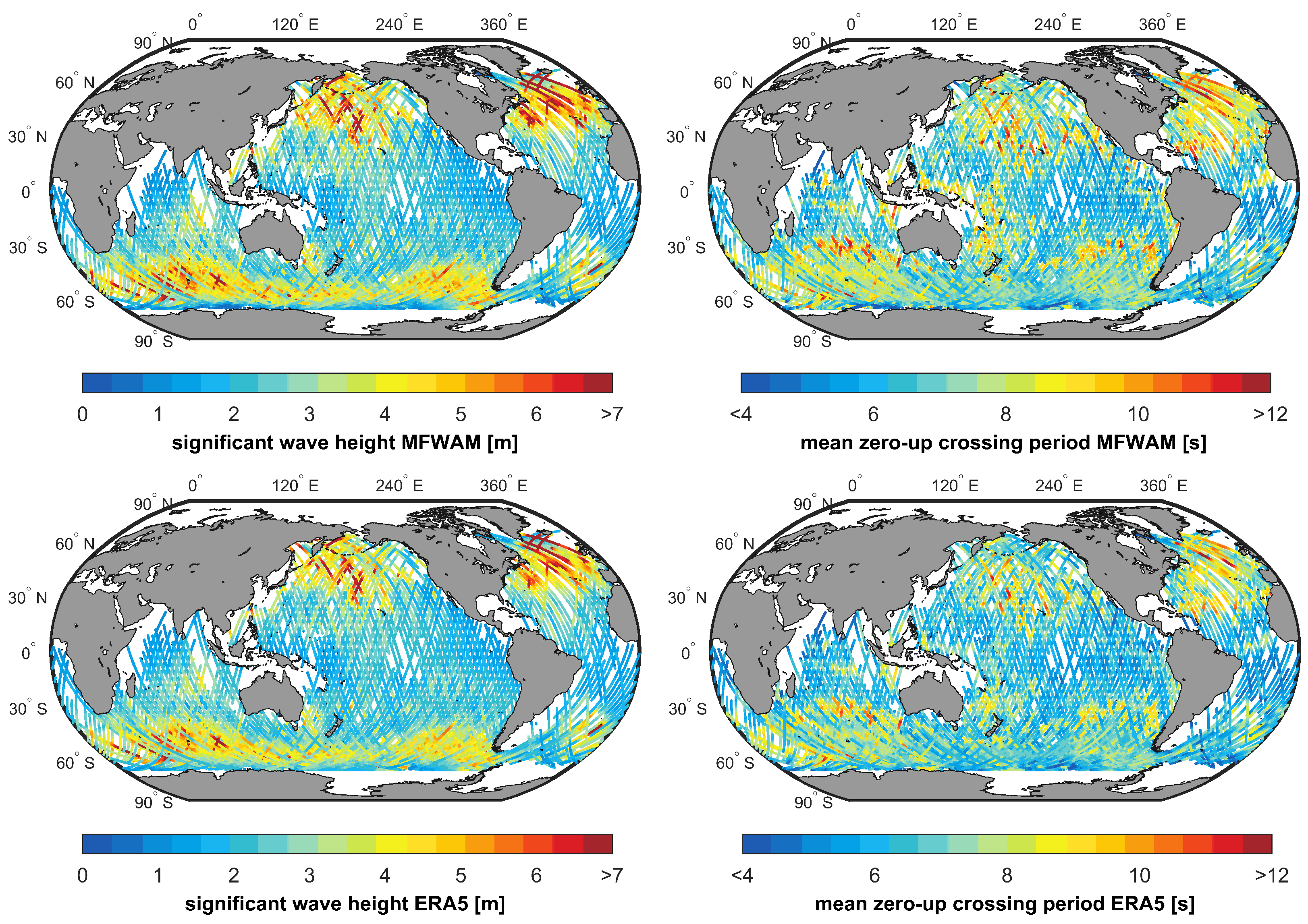
Figure 1. Examples of Sentinel-6A fully-focused SAR waveform-tail radargrams. Wind and wave conditions, given in the title of each panel, obtained from collocated ERA5 products.
Remotesensing 16 01292 g001
Figure 2. Interpolated significant wave height (left column) and mean zero-up crossing period (right column) parameters of MFWAM (top row) and ERA5 (bottom row) to Sentinel-6A tracks.
Remotesensing 16 01292 g002
Figure 3. Ratio of the σ υ w w , h f 2 wave orbital velocity variance of high-frequency waves (>0.58 Hz) to the σ υ w w 2 total wave orbital velocity variance versus wind speed. The colors represent the different fetches.
Remotesensing 16 01292 g003
Figure 4. Example of the along-track autocorrelation function, depicted in gray color, of a Sentinel-6A (S6A) fully-focused SAR waveform-tail radargram acquired for a scene characterized by moderate wind and wave conditions. The blue dashed line represents the Gaussian function. The yellow dash-dotted lines represent the Sentinel-6A azimuth cutoff estimate. Sea-state conditions are obtained from ERA5 products.
Remotesensing 16 01292 g004
Figure 5. Scatter plots of the azimuth cutoff estimated by Sentinel-6A in comparison to ERA5 (top panels) and MFWAM (bottom panels). In the left and right panels, color gradations correspond to wind speed and significant wave height, respectively. The square markers linked with solid gray lines depict the average value of points grouped every 50 m considering wave model-derived intervals. The gray dashed lines represent the scenario where the azimuth cutoff of the satellite and wave model would align perfectly.
Remotesensing 16 01292 g005
Figure 6. Examples of Sentinel-6A fully-focused SAR waveform-tail radargrams (left panels) and their along-track autocorrelation functions (right panels), illustrated in gray color. The blue dashed line represents the Gaussian function. The yellow, pink, and brown dash-dotted lines represent the Sentinel-6A, ERA5 and MFWAM azimuth cutoff estimates, respectively. Sea state conditions are obtained from ERA5 products.
Remotesensing 16 01292 g006
Figure 7. Examples of along-track autocorrelation functions, depicted in gray color, concerning SAR waveform-tail radargrams dominated by swells traveling in the cross-track direction (top left), at angle (top right and bottom left) and in the along-track direction (bottom right). The blue dashed line represents the Gaussian function. The yellow, pink, and brown dash-dotted lines represent the Sentinel-6A, ERA5 and MFWAM azimuth cutoff estimates, respectively. Sea-state conditions are obtained from ERA5 products.
Remotesensing 16 01292 g007
Figure 8. Example of the spectral autocorrelation function (gray solid line). The yellow circular marker represents the fall-off wavenumber identified as the intersection point between the gray dotted line, depicting the threshold line equal to five times the median spectral along-track autocorrelation function, and the blue solid line representing the seventh-order polynomial model. The pink and brown dash-dotted lines represent the fall-off wavenumber estimates from ERA5 and MFWAM, respectively. The yellow dash-dotted represents the Sentinel-6A fall-off wavenumber obtained from the spatial domain-derived azimuth cutoff estimate. Sea-state conditions are obtained from ERA5 products.
Remotesensing 16 01292 g008
Figure 9. Global maps of the azimuth cutoff as derived by ERA5 (top left), MFWAM (top right), Sentinel-6A from the spatial domain (SD) analysis (bottom left), and Sentinel-6A from the wavenumber domain (or Fourier Domain—FD) analysis (bottom right). Each map is accompanied by a histogram showing the distribution of the estimates on a logarithmic scale.
Remotesensing 16 01292 g009
Figure 10. Global maps of the velocity variance as derived by ERA5 (top left), MFWAM (top right), Sentinel-6A from the spatial domain (SD) analysis (bottom left), and Sentinel-6A from the wavenumber domain (or Fourier Domain—FD) analysis (bottom right). Each map is accompanied by a histogram showing the distribution of the estimates on a logarithmic scale.
Remotesensing 16 01292 g010
Figure 11. Global maps of the peak wave period and wind speed as obtained from ERA5 (top panels) and the velocity variance differences between ERA5 and Sentinel-6A in the spatial domain (SD) (mid left) and wavenumber domain (or Fourier Domain—FD) (mid right), MFWAM and Sentinel-6A in the spatial (bottom left) and wavenumber (bottom right) domains. Histograms of velocity variance differences accompany the middle and bottom panels.
Remotesensing 16 01292 g011
Table 1. Statistics of the differences and correlation coefficients between ERA5 and MFWAM wave parameters.
MFWAM−ERA5MeanStd. Dev.Corr. Coef.
Significant wave height [m]0.120.380.96
Mean zero-up crossing period [s]0.350.590.88
Table 2. Spatial domain analysis: statistics of the azimuth cutoff differences and correlation coefficients between Sentinel-6A and wave models based on a sensitivity analysis of the former to changes in wind speed, significant wave weight and a combination thereof. The values outside and inside parentheses represent ERA5 and MFWAM results, respectively.
CategoryPointsMean [m]Std. Dev. [m]Corr. Coef.
All data318,590 (318,541)−16.47 (−10.59)101.84 (96.70)0.67 (0.71)
Wind speed [m/s]
U10 < 568,811 (68,794)62.18 (63.08)91.07 (93.67)0.51 (0.51)
5 < U10 < 15237,359 (237,327)−32.65 (−27.71)90.23 (86.14)0.65 (0.70)
U10 > 1512,420 (12,420)−143.04 (−90.81)95.64 (88.83)0.65 (0.72)
Significant Wave Height [m]
Hs < 278,345 (79,377)12.19 (32.99)95.17 (107.22)0.07 (0.01)
2 < Hs < 5224,755 (217,442)−22.73 (−23.13)100.29 (87.98)0.48 (0.56)
Hs > 515,490 (21,722)−70.62 (−44.83)117.93 (90.75)0.29 (0.48)
Significant Wave Height [m] and Wind Speed [m/s]
2 < Hs and U10 < 536,167 (33,907)52.80 (70.36)94.28 (104.95)0.14 (0.03)
2 < Hs < 5 and 5 < U10 < 15188,088 (178,709)−35.72 (−36.46)91.30 (80.13)0.51 (0.58)
Hs > 5 and U10 > 158226 (8043)−126.12 (−87.94)98.00 (77.78)0.51 (0.70)
Table 3. Root mean square errors (RMSE) of the azimuth cutoff differences between Sentinel-6A (S6A) and wave model-derived values, calculated for varying numbers of samples considered in the spectral autocorrelation fitting.
Azimuth Cutoff Differences [m]RMSE
2050100
S6A-ERA5 102.1593.32106.69
S6A-MFWAM 99.0588.6396.23
Table 4. Wavenumber domain analysis: statistics of the azimuth cutoff differences and correlation coefficients between Sentinel-6A and wave models based on a sensitivity analysis of the former to changes in wind speed, significant wave weight and a combination thereof. The values outside and inside parentheses represent ERA5 and MFWAM results, respectively.
CategoryPointsMean [m]Std. Dev. [m]Corr. Coef.
All data311,640 (311,594)−41.68 (−38.53)83.50 (79.98)0.79 (0.81)
Wind speed [m/s]
U10 < 566,918 (66,902)−17.93 (−18.94)58.16 (57.01)0.68 (0.73)
5 < U10 < 15232,486 (232,456)−43.010 (−41.03)84.24 (82.20)0.71 (0.73)
U10 > 1512,236 (12,236)−146.30 (−98.16)100.79 (104.69)0.20 (0.26)
Significant Wave Height [m]
Hs < 275,068 (73,463)−21.9 (−9.87)75.83 (71.60)0.51 (0.52)
2 < Hs < 5221,198 (216,403)−40.26 (−38.98)79.66 (76.09)0.74 (0.76)
Hs > 515,374 (21,728)−158.71 (−131.49)79.38 (70.04)0.58 (0.62)
Significant Wave Height [m] and Wind Speed [m/s]
Hs < 2 and U10 < 534,721 (32,190)−14.5 (−1.55)61.11 (58.01)0.47 (0.47)
2 < Hs < 5 and 5 < U10 < 15185,075 (177,970)−42.65 (−40.34)82.21 (79.52)0.68 (0.69)
Hs > 5 and U10 > 158139 (8050)−180.21 (−139.01)83.70 (81.39)0.33 (0.30)
Disclaimer/Publisher’s Note: The statements, opinions and data contained in all publications are solely those of the individual author(s) and contributor(s) and not of MDPI and/or the editor(s). MDPI and/or the editor(s) disclaim responsibility for any injury to people or property resulting from any ideas, methods, instructions or products referred to in the content.

