CDEST: Class Distinguishability-Enhanced Self-Training Method for Adopting Pre-Trained Models to Downstream Remote Sensing Image Semantic Segmentation

Abstract

The self-supervised learning (SSL) technique, driven by massive unlabeled data, is expected to be a promising solution for semantic segmentation of remote sensing images (RSIs) with limited labeled data, revolutionizing transfer learning. Traditional ‘local-to-local’ transfer from small, local datasets to another target dataset plays an ever-shrinking role due to RSIs’ diverse distribution shifts. Instead, SSL promotes a ‘global-to-local’ transfer paradigm, in which generalized models pre-trained on arbitrarily large unlabeled datasets are fine-tuned to the target dataset to overcome data distribution shifts. However, the SSL pre-trained models may contain both useful and useless features for the downstream semantic segmentation task, due to the gap between the SSL tasks and the downstream task. To adapt such pre-trained models to semantic segmentation tasks, traditional supervised fine-tuning methods that use only a small number of labeled samples may drop out useful features due to overfitting. The main reason behind this is that supervised fine-tuning aims to map a few training samples from the high-dimensional, sparse image space to the low-dimensional, compact semantic space defined by the downstream labels, resulting in a degradation of the distinguishability. To address the above issues, we propose a class distinguishability-enhanced self-training (CDEST) method to support global-to-local transfer. First, the self-training module in CDEST introduces a semi-supervised learning mechanism to fully utilize the large amount of unlabeled data in the downstream task to increase the size and diversity of the training data, thus alleviating the problem of biased overfitting of the model. Second, the supervised and semi-supervised contrastive learning modules of CDEST can explicitly enhance the class distinguishability of features, helping to preserve the useful features learned from pre-training while adapting to downstream tasks. We evaluate the proposed CDEST method on four RSI semantic segmentation datasets, and our method achieves optimal experimental results on all four datasets compared to supervised fine-tuning as well as three semi-supervised fine-tuning methods.

1. Introduction

The vast availability of remote sensing images (RSIs) laden with rich information has opened the door to various Earth observation applications. How to extract information accurately and automatically from RSIs, especially through semantic segmentation or dense labeling, is one of the most interesting and long-standing problems [1,2]. This process is crucial for various applications such as urban planning, disaster monitoring, environmental protection, and agricultural management [3,4,5].

In the last decade, deep learning (DL)-based models have revolutionized RSI semantic segmentation by replacing hand-crafted features with data-driven features, achieving remarkable performance [6,7,8]. However, the high performance of these DL models relies on a critical assumption: the training and testing data should have similar distributions [9,10]. Unfortunately, RSIs obtained from different regions and time phases often exhibit significant distributional discrepancies [11,12]. In most cases, manual annotation and individual re-training of the semantic segmentation model is required for each RSI dataset [13].

To solve the inefficiency problem, researchers have developed transfer learning (TL) methods to adopt the models learned on a labeled dataset (source domain) to other datasets (target domain) with only a few labeled or even unlabeled samples [9,14]. Among them, representative methods include feature distribution alignment TL methods and data distribution alignment TL methods. The former type of method focuses on learning invariant features across domains by integrating the target and source data [15,16,17,18,19]; the latter directly modifies source or target data to reduce domain differences [20,21,22,23]. Although these TL methods have achieved good results on many public semantic segmentation datasets, this ‘local-to-local’ transfer paradigm suffers from the following major limitations: (1) The generalization ability and performance of the model are limited due to the inability to fully utilize large and diverse source datasets. (2) They rely on a high degree of similarity between the source and the target domains to satisfy the above basic assumption, which is difficult to guarantee in practical applications.

Recently, a new feature-learning paradigm, self-supervised feature learning (SSFL), has been widely used in remote sensing [24,25,26]. SSFL methods can learn abundant visual features directly from massive unlabeled data [27], which fundamentally shifts the TL paradigm from ‘local-to-local’ to ‘global-to-local’ [28,29]. The basic pipeline of the second TL paradigm is ‘pre-training + fine-tuning’ [30]. Specifically, the SSFL method is used to pre-train the model on a large-scale source domain dataset to learn global features, and then fine-tune it to adapt to a specific downstream task dataset. The key advantages of this paradigm are, first, with large and diverse datasets and well-designed SSFL methods, pre-trained models can learn powerful features with distinguishability, and which are crucial for a variety of downstream tasks such as semantic segmentation [31,32,33,34]. For example, FALSE [33] uses coarse judgment and fine calibration to construct positive and negative samples and obtain features that are more beneficial to downstream semantic segmentation tasks. IndexNet [32] and DenseCL [35] add a dense contrastive module in the pre-training stage to improve the performance of the semantic segmentation task. Second, since we can choose a source dataset similar to the target dataset at a low cost for pre-training, this paradigm can potentially alleviate the domain difference, and thus, ensure the performance of the learned features in the target RSI semantic segmentation task. However, due to the gap between the self-supervised pre-training task and the downstream semantic segmentation task, the pre-training model contains both relevant features that are useful for the downstream task and features that are irrelevant or even have a negative impact on the downstream task. Therefore, it is challenging to adapt the pre-trained model to the downstream task with only a small amount of downstream annotated data.

Traditional supervised fine-tuning is the most straightforward and most prevalent method to adapt self-supervised pre-trained models to specific downstream tasks [32,36,37,38,39]. However, during supervised fine-tuning, models could easily overfit with few labeled examples in downstream tasks, which prevents achieving higher semantic segmentation performance. This problem arises as the model strives to map a few training samples from the high-dimensional, sparse image space to the low-dimensional, compact semantic space defined by the downstream labels, resulting in degradation of the distinguishability. Unfortunately, the above mapping process is inherent to the objective of supervising fine-tuning.

To address the problem of overfitting, Chen et al. introduced a semi-supervised fine-tuning method that incorporates unlabeled data into supervised fine-tuning as a form of regularization [40]. Semi-supervised methods have been widely studied and can be broadly classified into consistency regularization-based methods, pseudo-labeling-based methods, and hybrid methods [41]. First, the basic idea of consistency-based regularization methods is to constrain various perturbations by using forced consistency loss [42,43,44]. For example, the unsupervised data augmentation (UDA) method generates a perturbed version of the data through data augmentation for unlabeled data, then feeds the data before and after augmentation into the network, and uses the KL dispersion (Kullback–Leibler divergence) loss to promote the consistency of the two outputs [44]. Second, the pseudo-labeling-based method generates pseudo-labels for unlabeled data and uses the high-confidence samples to guide model learning through filtering or weighting [45]. In such approaches, how to efficiently filter out reliable pseudo-labels is crucial for improving model performance but challenging. One representative approach is to build separate teacher and student models and optimize the label filtering results through iterations [46]. Another representative idea is to train multiple models and simultaneously generate multiple versions of pseudo-labels using different views of the data, and then improve the quality of pseudo-labels by exploiting the complementarity of the models [47]. Finally, hybrid semi-supervised methods incorporate the previously mentioned semi-supervised methods of consistent regularization, pseudo-labeling, or some other ideas [45]. For example, FixMatch effectively fuses the two ideas of consistent regularization and pseudo-labeling in a very concise manner [48]. Although these approaches help to alleviate overfitting, a larger number of training data and longer training processes significantly increase the risk of catastrophic forgetting [49,50,51], i.e., the model is more likely to completely forget distinguishability features learned during the pre-training process.

Unlike the above fine-tuning methods, this paper proposes the class distinguishability-enhanced self-training (CDEST) method for adopting SSL pre-trained models to downstream RSI semantic segmentation tasks. CDEST can mine supervisory information from both labeled and unlabeled data to provide effective guidance for fine-tuning. For labeled data, the proposed method employs a supervised fine-tuning and supervised contrastive learning (SCL) module to enhance the distinguishability and invariance of features. For unlabeled data, we first construct a self-training (ST) module to mine additional supervised information from unlabeled data to guide the fine-tuning in a semi-supervised learning manner, thus overcoming the overfitting problem. Secondly, we also design a semi-supervised contrastive learning (SSCL) module in the proposed method to further overcome the above-mentioned catastrophic forgetting problem. Note that the SCL module and the SSCL module of the proposed method utilize real labels and pseudo-labels, respectively, to guide contrastive learning. Compared with typical self-supervised contrast learning, these two modules can effectively avoid the problem of over-distinguishing between samples of the same class, thus achieving better inter-class distinguishability and intra-class invariance. We present experiments conducted on four datasets to demonstrate the effectiveness of our method.

The main contributions of this paper are as follows:

(1)

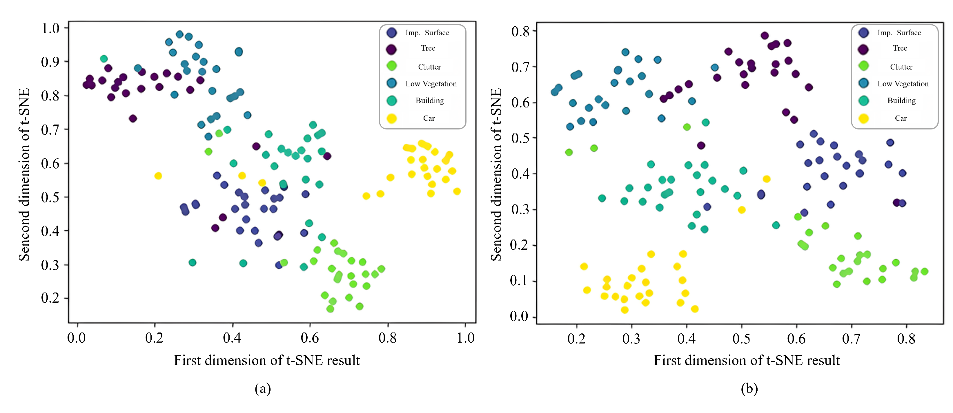
We propose a novel fine-tuning method to provide effective support for the most recent global-to-local transfer learning paradigm. By leveraging both labeled and unlabeled data to enhance the class distinguishability of features, our method can efficiently maintain useful features in self-supervised pre-trained models while adapting them to downstream semantic segmentation tasks.

(2)

We combine self-training and contrastive learning mechanisms and design three modules to mine effective supervisory information from both labeled and unlabeled data, to guide model fine-tuning to overcome overfitting and catastrophic forgetting issues.

(3)

We evaluate our proposed method on two public datasets and two realistic datasets. The experimental results show that our method outperforms both traditional supervised fine-tuning and several representative semi-supervised fine-tuning methods.

2. Methodology

This section introduces our proposed class distinguishability-enhanced self-training (CDEST) method for adapting self-supervised pre-trained models to downstream semantic segmentation tasks. The overall framework of the proposed CDEST method is presented in Section 2.1. Then, the three important modules of CDEST, the supervised comparative learning (SCL) module, the self-training (ST) module and the semi-supervised comparative learning (SSCL) module, are described in Section 2.2, Section 2.3 and Section 2.4, respectively.

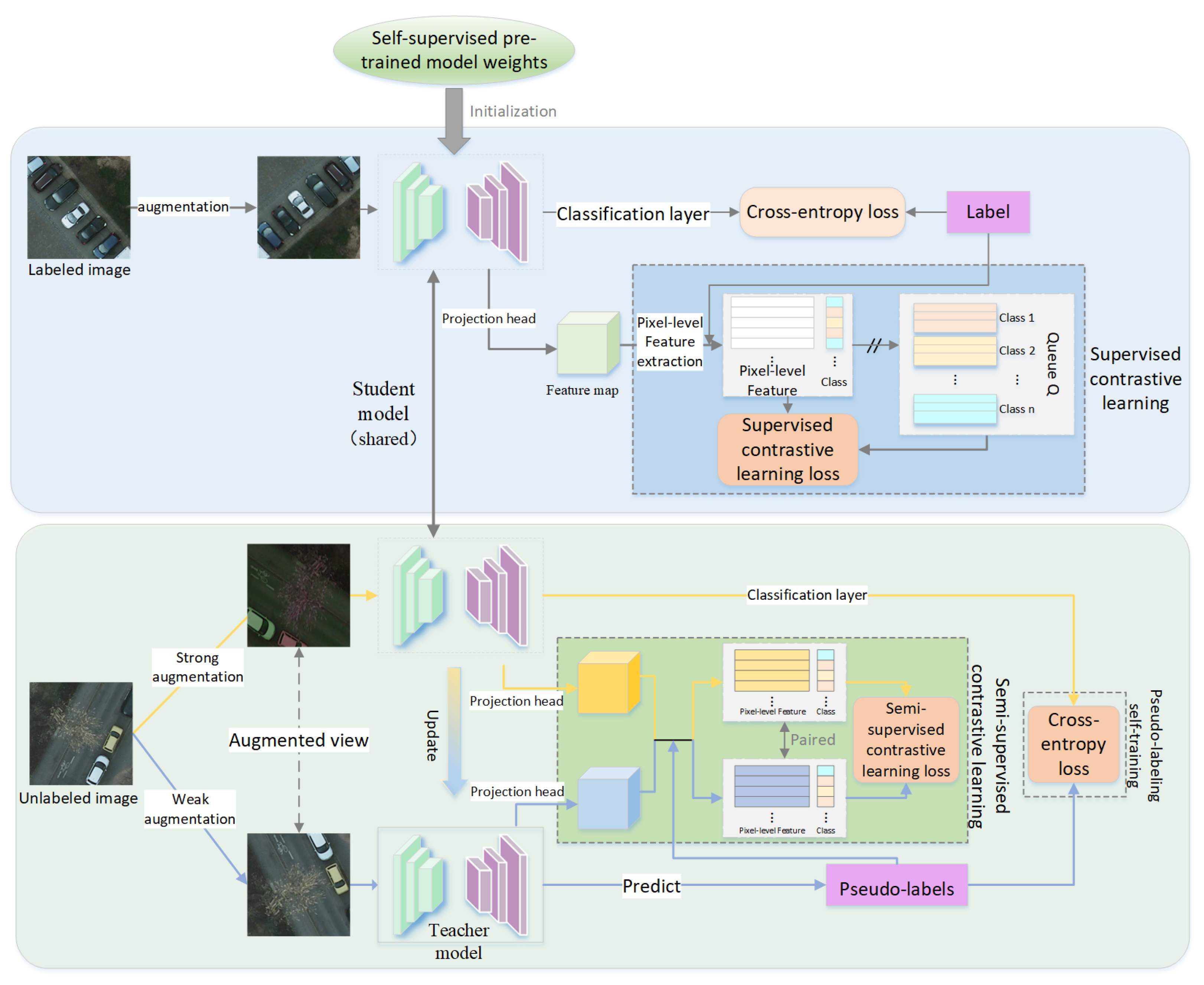
2.1. The Overall Framework of CDEST

The overall framework of the fine-tuning method CDEST proposed in this paper is shown in Figure 1. For an encoder–decoder architecture model initialized with pre-trained weights, CDEST uses a small amount of labeled data and a large amount of unlabeled data to fine-tune it to the downstream semantic segmentation tasks.

For labeled data, in addition to being used for basic supervised learning, CDEST feeds it into the SCL module to enhance feature distinguishability. Unlike typical contrastive learning methods [27,52,53,54], the SCL module has two primary differences: firstly, it selects individual pixels instead of image patches to construct positive and negative sample pairs, facilitating the learning of fine-grained features that are more suitable for downstream semantic segmentation tasks; secondly, the SCL module treats all samples of the same class as positive samples and only samples of different classes as negative ones, avoiding the problem of over-distinguishing between samples of the same class in typical self-supervised contrastive learning methods [33,55], thus contributes to enhancing the inter-class distinguishability and intra-class consistency of the learned representations.

The unlabeled data can be utilized by the ST and SSCL modules to provide additional supervisory information for fine-tuning. The significance of these two modules is to avoid model overfitting and further improve the semantic segmentation performance. Firstly, the ST module is crucial for the proposed method to be able to utilize unlabeled data. This module takes the downstream model initialized with pre-trained weights as the student model and the supervised fine-tuned version as the teacher model. During self-training, the teacher model generates pseudo-labels for all unlabeled data to train the student model, thereby enhancing its semantic segmentation performance. In this process, the teacher model periodically updates itself with the student model’s parameters instead of relying on gradient-based parameter optimization. Secondly, SSCL has the same core objectives as the above SCL module but leverages pseudo-labels instead of manual labels to guide the construction of positive and negative samples.

2.2. Supervised Contrastive Learning Module with Labeled Data

Enhancing the distinguishability between classes and reducing the variance within classes of the learned representations are key to improving the performance of RSI classification [56,57,58]. Ideally, this goal could easily be achieved by supervised contrastive learning methods [59] that bring samples of the same class closer and separate samples of different classes in the representation space. However, supervised contrastive learning based on RSIs faces two major challenges: first, the redundancy of RSIs (i.e., RSIs containing massive numbers of almost identical pixels) leads to very low computational efficiency in contrastive learning. Second, the number of geographic elements in RSIs varies greatly [60], leading to an extreme class imbalance encountered during contrastive learning. In this case, the model tends to ignore the samples with small proportions, thus making it difficult to improve the distinguishability within these categories as well as with other categories [34].

To tackle the issue of computational inefficiency, this paper proposes the SCL module, which samples pixel-level features in a low-dimensional and compact representation space, rather than sampling original pixels in the high-dimensional and redundant image space. To address the problem of class imbalance, the SCL module maintains a dynamic queue to store massive amounts of pixel features categorically. This ensures that each training batch for contrastive learning draws samples with balanced categories and positive and negative ratios. The detailed implementation process of the proposed SCL module for a small amount of labeled data is detailed below:

(1)

Image encoding to generate feature maps

Given a labeled image x, we first feed it into the student semantic segmentation network to obtain the feature map $d\left(e\right(\mathit{x}\left)\right)$, which is the output of the previous layer of the final classification layer. Since we used a self-supervised pre-trained DeepLabV3+ model [61] provided by [31] as the student network in this paper, $e(·)$ and $d(·)$ correspond to the encoder and decoder of this model, respectively. Inspired by previous work [53,62], we also utilized a projection head module $g(·)$ for applying a non-linear mapping to the feature map $d\left(e\right(\mathit{x}\left)\right)$ before contrastive learning to improve the performance of the learned representations, where $g(·)$ consists of two 1 × 1 convolutional layers (the first convolutional layer denoted $Con{v}^1$, and the second convolutional layer denoted $Con{v}^2$) and a ReLU layer (denoted R). The final feature map used to collect samples for contrastive learning is shown in the following equation:

$${\mathit{f}}_{map}=g\left(d\left(e\left(\mathit{x}\right)\right)\right)=Con{v}^{2}R\left(Con{v}^{1}d\left(e\left(\mathit{x}\right)\right)\right)$$

(1)

(2)

Sample queue construction and update

To address the class imbalance, the SCL module creates a queue Q that stores an equivalent number of samples from each category for contrastive learning. The size of Q is $C\times N_q\times K$, where C stands for the total number of categories, $N_q$ represents the maximum number of pixel-level feature vectors retained for each category, and K is the dimensionality of the feature map ${\mathit{f}}_{map}$. In the construction phase of Q, the SCL module randomly samples the feature vectors of pixels of each image $\mathit{x}$ and adds them to Q by class, where the class information is obtained from the pixel-level semantic segmentation label $\mathit{y}$ corresponding to $\mathit{x}$. To diminish feature redundancy, the maximum number of each class of feature vector sampled from each image is $C_{Max}$. In the update phase, the SCL module traverses images continuously, gathering new feature vectors corresponding to pixels of images in various classes. These vectors are used to replace the previously stored samples of the same class, following a first-in-first-out principle. The full queue is perfectly class-balanced since the maximum number of samples in each category in Q is $N_q$.

(3)

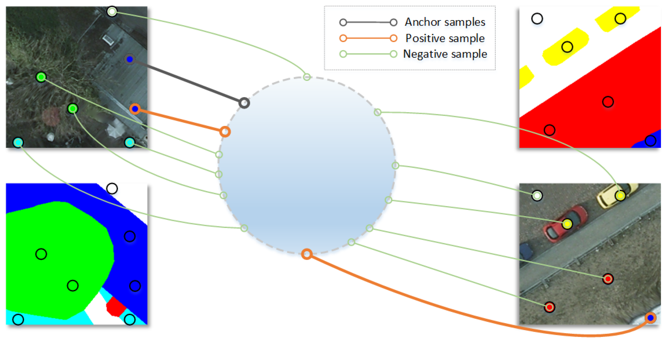
Constructing positive and negative samples

This module aims to enhance the distinguishability between classes and reduce the variance within classes of the learned representations by supervised contrastive learning (Figure 2). Since this process is achieved by bringing positive sample features closer and pushing negative sample features farther away, the way of constructing positive and negative samples is crucial for the above purpose. Note that either positive or negative samples are relative concepts, and their baseline samples are usually referred to as anchor samples.

To achieve balanced classes, we first try to randomly select $N_A/C$ pixel-level sample features as anchor samples for each class based on labels from the current batch of training data, where $N_A$ is a hyperparameter indicating the total number of anchor samples to be selected and C denotes the number of classes. If a class has fewer than $N_A/C$ samples in the current training batch, we select all those samples and continue to randomly select the same class of samples from Q as a supplement until obtaining $N_A/C$ anchor samples.

Then, for the i-th sample of all $N_A$ anchor samples, we select samples from the queue Q of the same class to construct its positive sample set $P\left(i\right)$ and samples of a different class for the negative sample set $N\left(i\right)$. The resulting set of positive and negative samples is denoted as $O\left(i\right)$.

(4)

Supervised contrastive loss

Once the anchor samples and positive and negative samples are specified, the model can be trained by optimizing the supervised contrastive loss function $L_{con}^{lbl}$, as defined in Equation (2):

$${\mathcal{L}}_{con}^{lbl}=\sum _{i=1}^{N_A}-\frac{1}{\left|P\right(i\left)\right|}\sum _{p\in P\left(i\right)}\left(log\frac{exp(z_i·z_p/\tau )}{{\sum }_{o\in O\left(i\right)}exp(z_i·z_o/\tau )}\right)$$

(2)

where $N_A$ represents the number of anchor samples, while $\left|P\right(i\left)\right|$ indicate the size of the positive sample set $P\left(i\right)$. Then, $z_i$, $z_p$, and $z_o$ denote the feature of the i-th anchor sample, the p-th positive sample in $P\left(i\right)$, and the o-th sample in $O\left(i\right)$, respectively.

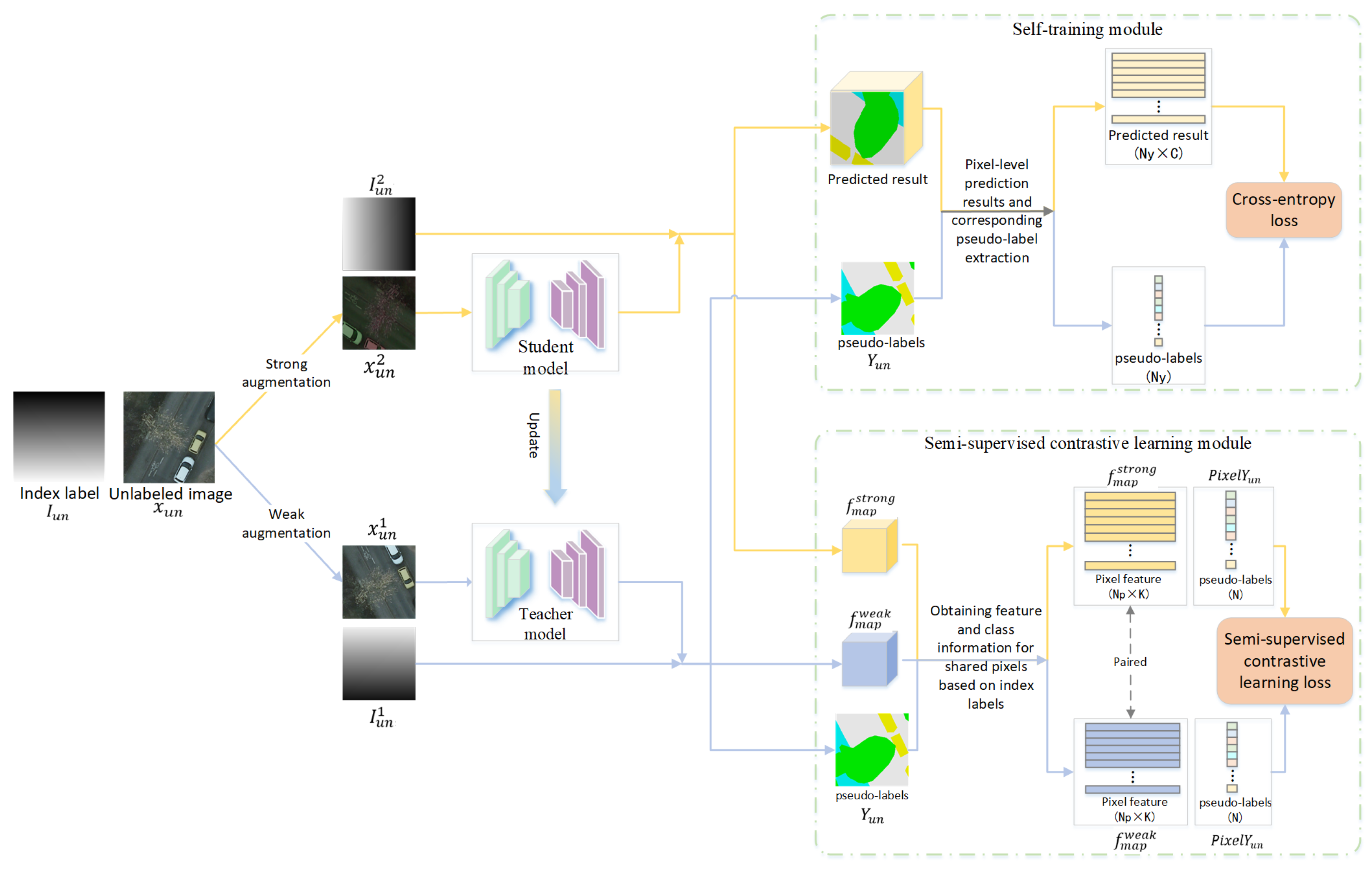
2.3. Self-Training Module with Unlabeled Data

To mine supervised information from unlabeled data to provide effective guidance for model fine-tuning, we introduce semi-supervised learning mechanisms including knowledge distillation [40] and self-training [46,63] to design the ST module.

The core idea of this module is to use unlabeled data and its pseudo-labels as a medium to transfer knowledge from one model (called the teacher model) to another model (the student model). During self-training, the predictions of the teacher model are relatively reliable and used as pseudo-labels since it takes input data with no significant perturbations applied. At the same time, the student model takes significantly perturbed data as input and is asked to obtain predictions consistent with the output of the teacher model. In this way, the useful features in the teacher model that facilitate the semantic segmentation task are gradually distilled into the student model. Then, when the student network outperforms the teacher network it is used again as a new teacher network. Through multiple iterations, the student model is continuously optimized and achieves better performance in the downstream task of semantic segmentation.

The implementation flow of the ST module is shown in Figure 3. Specifically, for an unlabeled image ${\mathit{x}}_{un}\in {\mathbb{R}}^{h\times w\times 3}$, the ST module firstly utilizes both weak and strong types of data augmentation to generate two views ${\mathit{x}}_{un}^1$ and ${\mathit{x}}_{un}^2$ of ${\mathit{x}}_{un}$, respectively. Each type of augmentation contains two main types of image processing operations: color augmentation operations (i.e., color distortion, random noise addition, etc.) and spatial augmentation operations (random rotation, flip, random crop, and zoom, etc.). Compared to strong augmentation, all operations of weak augmentation are less intense to preserve more original information of the data. Then, the weakly augmented result ${\mathit{x}}_{un}^1$ is fed into the teacher model to obtain high-quality pseudo-labels ${\mathit{Y}}_{un}$. The strongly augmented result ${\mathit{x}}_{un}^2$, after significant perturbation, is used as an input to the student model to obtain the prediction ${\mathit{y}}_{un}$. Finally, the ST model uses the cross-entropy loss function to measure the consistency between the outputs (${\mathit{Y}}_{un}$, ${\mathit{y}}_{un}$) of the two models and optimizes the student model by minimizing the loss value.

However, ${\mathit{Y}}_{un}$ and ${\mathit{y}}_{un}$ are not directly comparable because the spatial augmentation operations in the above data augmentations break the correspondence of pixels in the paired results (${\mathit{x}}_{un}^1$, ${\mathit{x}}_{un}^2$). To address this issue, we generate the corresponding index label ${\mathit{I}}_{um}\in {\mathbb{R}}^{h\times w}$ to record the position encoding of all pixels in ${\mathit{x}}_{un}$, following a row-first, column-second order. Specifically, the values of ${\mathit{I}}_{um}$ are in the range [1, $h\times w$]. By having ${\mathit{I}}_{um}$ undergo the same spatial augmentation operation as ${\mathit{x}}_{un}$, we can determine the pixel correspondence between (${\mathit{Y}}_{un}$, ${\mathit{y}}_{un}$) based on the two augmented views (${\mathit{I}}_{um}^1$, ${\mathit{I}}_{um}^2$) of index label ${\mathit{I}}_{um}$. Consequently, only labels of pairs of pixels are extracted for calculating the cross-entropy loss $L_{ce}^{un}$, where the number of pairs of pixels $N_y$ is less than or equal to $h\times w$.

2.4. Semi-Supervised Contrastive Learning Module with Unlabeled Data

Like the SCL module, this module also aims to enhance the distinguishability between classes and reduce the variance within classes of the learned representations. The framework of the SSCL module is shown in Figure 3, and its workflow includes the following five main steps:

(1)

Generate index labels: Given an unlabeled image ${\mathit{x}}_{un}\in {\mathbb{R}}^{h\times w\times 3}$, we generate the corresponding index label ${\mathit{I}}_{um}\in {\mathbb{R}}^{h\times w}$ to facilitate the subsequent determination of pixel correspondences from different augmentation results. The specific details of the index label are consistent with those described in the ST module above.

(2)

Data augmentation: Before feeding the data into the student and teacher models, we preprocess each pair of data (${\mathit{x}}_{un}$, ${\mathit{I}}_{um}$) with weak and strong types of augmentation to generate (${\mathit{x}}_{un}^1$, ${\mathit{I}}_{um}^1$) and (${\mathit{x}}_{un}^2$, ${\mathit{I}}_{um}^2$). The design of the two types of data enhancements here is consistent with that in the ST module.

(3)

Feature map extraction: To obtain the pixel features for contrastive learning, we feed $x_{un}^1$ into the teacher network to generate feature maps ${\mathit{f}}_{map}^{weak}$ and ${\mathit{Y}}_{un}$. At the same time, we feed $x_{un}^2$ into the student model to generate K-dimensional ${\mathit{f}}_{map}^{strong}$. The specific generation process of ${\mathit{f}}_{map}^{weak}$ and ${\mathit{f}}_{map}^{strong}$ is consistent with that described by Equation (1).

(4)

Acquisition of pairwise pixel features and their class information: Based on the index labels ${\mathit{I}}_{um}^1$ and ${\mathit{I}}_{um}^2$, we can determine the correspondence between the pixels on the feature maps ${\mathit{f}}_{map}^{weak}$, ${\mathit{f}}_{map}^{strong}$, and ${\mathit{Y}}_{un}$ to obtain all the paired pixels and their labels. Then, to reduce the redundancy, all paired pixel features are randomly filtered and only $N_P$ pixel features are finally retained.

(5)

Loss function for semi-supervised contrastive learning: For each anchor sample ${\mathit{f}}_k^{strong}$, the positive sample is the pixel feature ${\mathit{f}}_k^{weak}$ paired with it, and its negative samples $A\left(k\right)$ are all the pixel features in the current training batch data that are not in the same class as ${\mathit{f}}_k^{strong}$. The class information of these samples is obtained from the pseudo-label ${\mathit{Y}}_{un}$. The final semi-supervised contrastive learning loss is defined as follows:

$${\mathcal{L}}_{con}^{unbl}=\frac{1}{N_p}\sum _{k=1}^{N_p}-log\frac{exp({\mathit{f}}_k^{strong}·{\mathit{f}}_k^{weak}/\tau )}{{\sum }_{a\in A\left(k\right)}exp({\mathit{f}}_k^{strong}·{\mathit{f}}_a/\tau )}$$

(3)

where $N_p$ denotes the total number of paired pixel features selected in the whole batch, $A\left(k\right)$ denotes the pixel features of other categories among the $N_p$ pixel features whose pseudo-labeling categories do not belong to the same sample class as ${\mathit{f}}_k^{strong}$, and $\tau$ is a temperature hyperparameter.

2.5. The Complete Loss Function of the CDEST Method

In summary, the complete loss function $\mathcal{L}$ of the proposed method consists of four parts:

$$\mathcal{L}={\lambda }_1{\mathcal{L}}_{ce}^{lbl}+{\lambda }_2{\mathcal{L}}_{con}^{lbl}+{\lambda }_3{\mathcal{L}}_{ce}^{un}+{\lambda }_4{\mathcal{L}}_{con}^{un}$$

(4)

where ${\mathcal{L}}_{ce}^{lbl}$ is the supervised learning loss for labeled data, using the cross-entropy loss function; ${\mathcal{L}}_{con}^{lbl}$ is the supervised contrastive learning loss for labeled data, as described in Equation (2); ${\mathcal{L}}_{ce}^{un}$ is the supervised learning loss for unlabeled data, also using the cross-entropy loss function; ${\mathcal{L}}_{con}^{un}$ is the semi-supervised contrastive learning loss for unlabeled data, as described in Equation (3). In addition, the coefficients ${\lambda }_1$, ${\lambda }_2$, ${\lambda }_3$, and ${\lambda }_4$ are empirical hyperparameters. Since the value of the contrastive learning loss is usually significantly larger than both supervised and semi-supervised loss values, we set the coefficients ${\lambda }_2$ and ${\lambda }_4$ to 0.2 for the former, and the coefficients ${\lambda }_1$ and ${\lambda }_3$ to 1.0 for the latter. In this way, the response of different losses to model fine-tuning can be better balanced.

3. Experiments

3.1. Data Description

We evaluated our proposed CDEST and the other compared methods using four RSI semantic segmentation datasets. Two of these datasets, the International Society for Photogrammetry and Remote Sensing (ISPRS) Potsdam dataset [64] and the Deep Globe Land Cover Classification (DGLCC) dataset [65], are publicly accessible. The other two are real-world datasets collected from Hubei and Xiangtan in China [31], characterized by the same spatial resolution but varying feature distributions. The details of these diverse datasets are outlined below.

(1)

ISPRS Potsdam Dataset: The Potsdam dataset [64] includes 38 high-resolution (HR) aerial images with a size of 6000 × 6000 pixels. Each image features a spatial resolution of 0.05 m, encompassing four spectral bands: red, blue, green, and near-infrared reflectance (NIR). The dataset is annotated with six categories: low vegetation, trees, buildings, impervious surfaces, cars, and others. For training purposes, 24 images are cropped into 13,824 patches as samples, each 256 × 256 pixels in size, with 1% labeled. For testing, 1500 labeled patches of 256 × 256 size were randomly selected from the cropped results of the remaining 14 images.

(2)

DGLCC Dataset: The DGLCC [65] dataset consists of HR satellite images, each 2448 × 2448 pixels in size. The dataset is annotated with seven categories: urban, agriculture, rangeland, forest, water, barren, and unknown. For training, we randomly selected 730 images and cropped them into patches of 512 × 512 pixels, with 1% labeled. The remaining 73 images were cropped into patches of $512\times 512$ pixels and used as testing samples.

(3)

Hubei Dataset: The Hubei dataset consists of images acquired from the Gaofen-2 satellite, covering the province of Hubei, China. These RGB images measure 13,889 × 9259 pixels and have a spatial resolution of 2 m. The dataset includes annotations in ten categories: background, farmland, urban, rural areas, water, woodland, grassland, other artificial facilities, roads, and others. We processed 34 images for training and 5 for testing, cropping them into 256 × 256-pixel patches to obtain the final samples. The number of samples is detailed in

Table 1. Description of the four datasets used in our experiment.

Datasets	Potsdam	DGLCC	Hubei	Xiangtan
Number of categories	6	7	10	9
Sample size (pixels)	256 × 256	512 × 512	256 × 256	256 × 256
Spatial resolution (m)	0.05	0.5	2	2
Number of labeled training samples	138	182	664	160
Number of unlabeled training samples	13,686	18,066	65,807	15,891
Number of testing samples	1500	1825	9211	3815

.

(4)

Xiangtan Dataset: The Xiangtan dataset consists of images also sourced from the Gaofen-2 satellite, covering the city of Xiangtan, China. This dataset is annotated with nine categories: background, farmland, urban, rural areas, water, woodland, grassland, road, and others. We processed 85 images for training and 21 for testing, cropping them into 256 × 256-pixel patches to generate the final samples. The number of samples is detailed in Table 1.

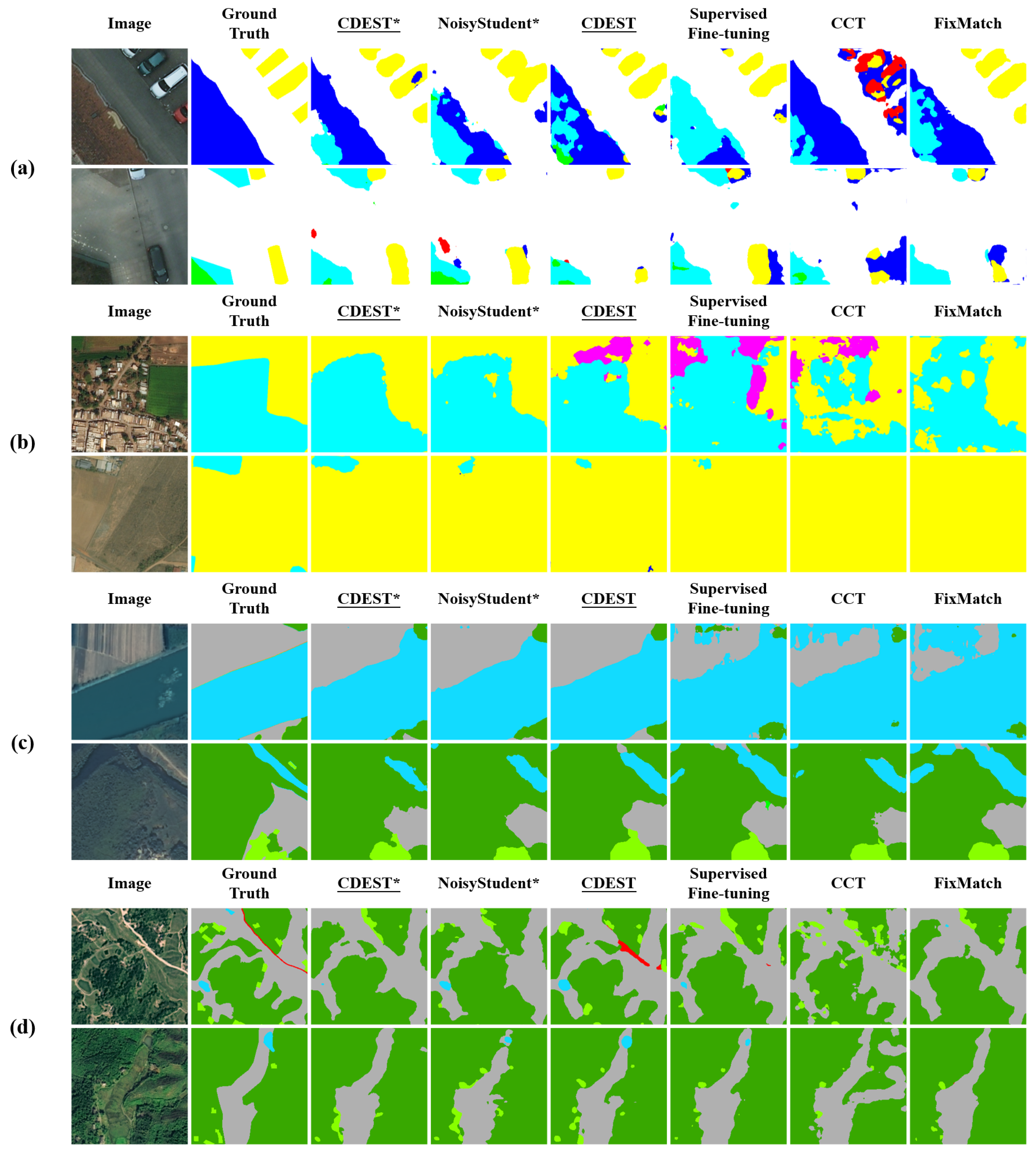
3.2. Comparison Experiments and Baseline

To verify the effectiveness of the proposed CDEST in fine-tuning the pre-trained model to downstream semantic segmentation tasks, we compared CDEST with typical supervised fine-tuning methods and several representative semi-supervised learning methods, including the cross-consistency training (CCT) method [33], the FixMatch method [48], and the NoisyStudent method [31]. The specific methods used for comparison are summarized as follows.

(1)

Supervised fine-tuning: Fine-tuning the model to downstream semantic segmentation tasks using only labeled data.

(2)

CCT: A semi-supervised fine-tuning method based on the consistency assumption that the model should be able to obtain stable and consistent predictions based on inputs containing small perturbations. Specifically, the CCT consists of an encoder, a main decoder, and several auxiliary decoders. The labeled data are used directly to train the encoder and the main decoder. For the features extracted by the encoder from the unlabeled data, their original versions are used as inputs to the main decoder, while the versions with added perturbations (e.g., added noise, dropped features, random rotations, etc.) are used as inputs to the auxiliary decoders. Then, by requiring the predictions of the primary and secondary decoders to be identical, the use of unlabeled data is achieved to enhance the robustness of the model itself and its adaptability to downstream tasks.

(3)

FixMatch: A semi-supervised fine-tuning method that incorporates the consistency constraint assumption and the idea of pseudo-label training. For annotated data, FixMatch performs normal supervised semantic segmentation training; for unlabeled data, FixMatch generates pseudo-labels for unlabeled images that are weakly augmented (e.g., random flip and shift) and discards those that are not predicted with high confidence. It then trains the model to complete semantic segmentation tasks by predicting the same pseudo-labels for the strongly augmented (e.g., Cutout [66] and AutoAugment [67]) versions of the same images.

(4)

NoisyStudent: A self-training semi-supervised method based on distillation learning, which leverages massive unlabeled data to improve the accuracy and robustness of the task model, NoisyStudent consists of the following steps: (I) It initializes the encoder part of the semantic segmentation model with a self-supervised pre-trained model and trains the teacher model on the annotated data. (II) It generates pseudo-labels by using the teacher model to predict the unlabeled data. (III) It selects the high-confidence predictions from the unlabeled data and trains the student model with the annotated data and the selected predictions. It also adds noise to the student model during training, such as random noise, color distortion, and data augmentation via RandAugment [68]. These noisy operations are more intense and diverse than the ones used in the normal semantic segmentation training, to make the student model more robust to noise. (IV) It makes the student model the new teacher model to predict the unlabeled data. (V) It repeats (III) and (IV) until convergence.

In the above methods, supervised fine-tuning only uses labeled samples (i.e., 1% of the training set) for training, while the rest of the semi-supervised methods and the proposed CDEST additionally use unlabeled samples (99% of the training set) in the training process.

3.3. Implementation Details

The experiment employed the Adam optimizer with an initial learning rate of 0.001 and adopted a polynomial decay strategy for learning rate adjustment. For a fair comparison, we set the total batch size at 16 for all fine-tuning methods. In the semi-supervised approaches, we set the batch size to 4 for labeled data and 12 for unlabeled data. Additionally, other shared hyperparameters and data augmentation strategies were aligned as consistently as possible across the various methods.

During training, we performed 16,000 iterations for supervised fine-tuning methods using only a small number of labeled samples, and 32,000 iterations for other semi-supervised methods that additionally use a large number of unlabeled samples. Specifically, we trained the NoisyStudent method, which employs a multi-round iterative self-training strategy, for n × 16,000 iterations, continuing until a decline in accuracy was observed (where n is not a fixed value). During testing, we used the Kappa and overall accuracy (OA) metrics to assess the fine-tuned models on four downstream semantic segmentation tasks.

3.4. Experimental Results

In this section, we fine-tuned the same self-supervised pre-trained model using the proposed CDEST method as well as the four comparative methods mentioned above on four semantic segmentation downstream tasks separately. The results in

Table 2. Comparison of results from four RSI semantic segmentation tasks. Bold numbers represent the maximum value under this indicator.

Methods	Potsdam		DGLCC		Hubei		Xiangtan
	Kappa	OA	Kappa	OA	Kappa	OA	Kappa	OA
Supervised fine-tuning	72.01	78.21	68.03	80.42	53.10	63.04	72.92	82.81
CCT	70.50	76.91	66.68	79.59	53.07	62.92	71.78	82.26
FixMatch	73.15	78.95	67.26	80.22	52.25	62.55	73.20	83.04
CDEST	74.85	80.37	68.47	81.14	55.04	64.67	73.39	83.26
NoisyStudent *	75.46	80.86	70.34	81.92	54.41	63.71	73.18	82.97
CDEST *	75.65	80.98	71.74	82.45	54.91	64.54	73.23	83.02

* Fine-tuning methods that use the multi-round iterative self-training strategy continue to train until accuracy degrades.

indicate that CDEST achieved enhanced metrics on each dataset compared to baseline methods.

On the Hubei dataset, our method outperforms the supervised fine-tuning, CCT, FixMatch, and NoisyStudent by 3.7%, 3.7%, 5.3%, and 1.2%, respectively, in Kappa, without using the multi-round self-training strategy. Similarly, for the Potsdam dataset, CDEST improves in both Kappa and OA metrics over the supervised fine-tuning, CCT, and FixMatch methods. Employing a multi-round self-training strategy further enhances CDEST’s performance, surpassing that of the NoisyStudent method. The visualized result is shown in Figure 4.

The results of the four datasets show that semi-supervised fine-tuning methods, which leverage supervised information from additional unlabeled data and its pseudo-labels, do not consistently improve the performance of downstream task models. For instance, in the DGLCC and Hubei datasets, the supervised fine-tuning approach, utilizing merely 1% labeled samples, outperforms the semi-supervised CCT and FixMatch methods that use 99% additional unlabeled samples. The main reason behind this is that the noise in pseudo-labels of unlabeled data inevitably provide incorrect supervisory information for fine-tuning, potentially leading the model to misidentify various objects or scenes in RSIs and diminish the inter-class distinguishability of the learned features. Furthermore, research has demonstrated that deep learning models tend to overfit toward incorrect labels more than toward correct ones [69,70]. Unlike the above semi-supervised fine-tuning methods, our method also utilizes these noise labels to guide the contrastive learning signal construction rather than only using these noise labels for supervised learning. In this way, CDEST is more robust to noise labels, and thus, achieves optimal performance on all four datasets.

4. Discussions

4.1. Ablation Study

In this section, we perform ablation experiments to investigate the effectiveness of three main modules of our proposed CDEST, including a supervised contrastive learning (SCL) module, a self-training (ST) module, and a semi-supervised contrastive learning (SSCL) module. The corresponding loss functions of these three modules are ${\mathcal{L}}_{con}^{lbl}$, ${\mathcal{L}}_{ce}^{un}$, and ${\mathcal{L}}_{con}^{un}$, respectively. The specific experimental results on the Potsdam dataset are shown in

Table 3. Results of ablation experiments on the Potsdam dataset, exploring the effectiveness of the modules of the proposed CDEST.

${\mathcal{L}}_{\mathit{ce}}^{\mathit{lbl}}$	${\mathcal{L}}_{\mathit{con}}^{\mathit{lbl}}$	${\mathcal{L}}_{\mathit{ce}}^{\mathit{un}}$	${\mathcal{L}}_{\mathit{con}}^{\mathit{un}}$	Kappa/OA
✔				72.16/78.22
✔	✔			72.80/78.79
✔		✔		74.10/79.81
✔			✔	72.22/78.27
✔	✔	✔		74.86/80.33
✔	✔		✔	73.39/79.20
✔		✔	✔	74.47/80.11
✔	✔	✔	✔	74.85/80.37

.

The experimental results show that all three modules help improve the performance of the fine-tuned model in the semantic segmentation downstream task. Among them, the ST module (i.e., ${\mathcal{L}}_{ce}^{un}$) contributes the most to the model performance improvement, which indicates that the semi-supervised method based on the idea of self-training is simple but effective.

For the SCL and SSCL modules, the primary objective of their design is to enhance the inter-class distinguishability of the learned features. To confirm the achievement of this objective, we randomly selected pixel features from all classes in the Potsdam dataset’s test set and visualized them using the t-SNE method. As shown in Figure 5a, without the SCL and SSCL modules, the pixel features of several classes appear indistinct. Conversely, with the integration of the SCL and SSCL modules, the fine-tuned model more effectively distinguishes between all pixel classes (Figure 5b), illustrating the significance of these two modules in enhancing inter-class feature distinguishability.

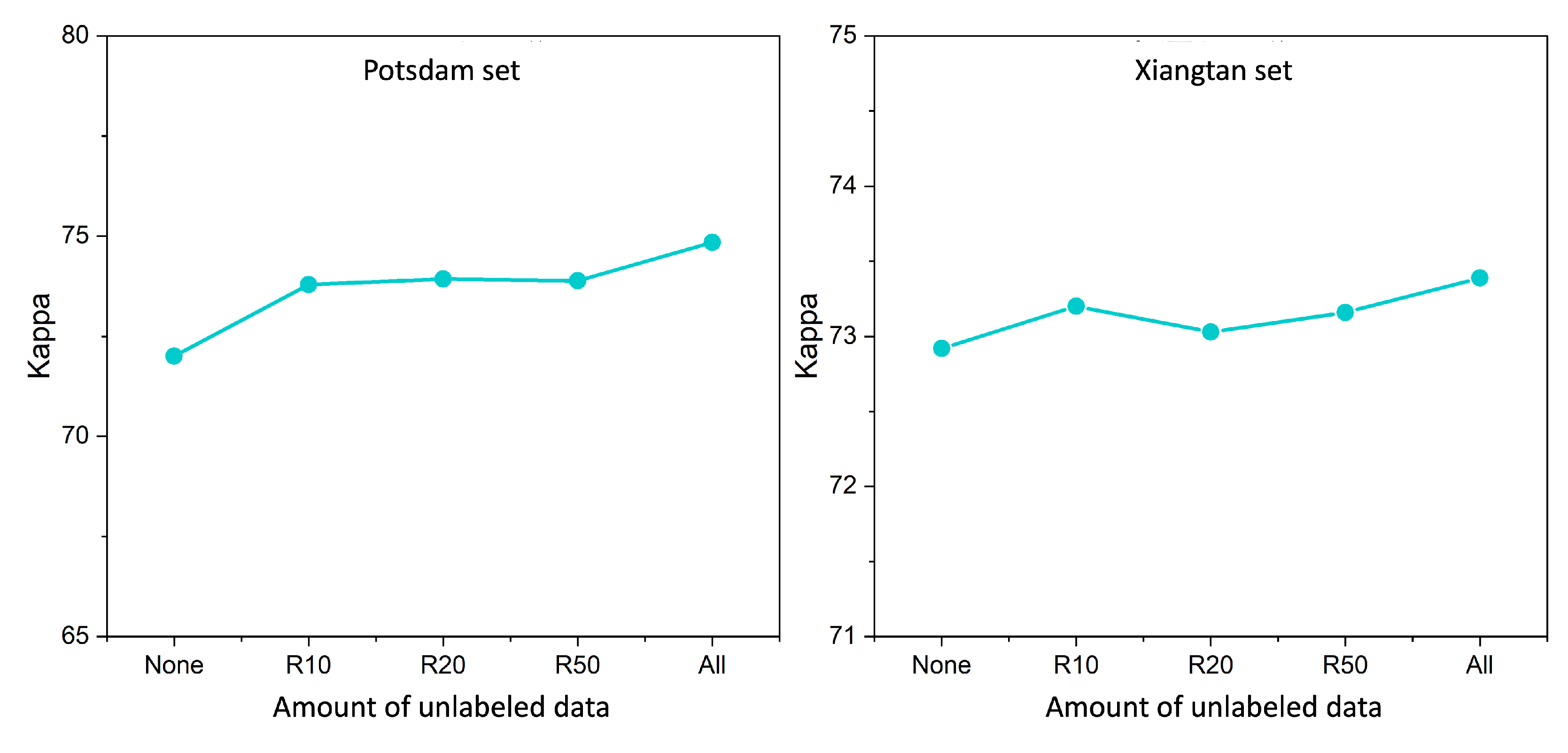
4.2. Study of the Quantity of Unlabeled Data

The quantity of unlabeled samples plays a critical role in the efficacy of the proposed method. To evaluate the impact of this factor on the performance of CDEST, we conducted a series of comparative experiments using the Potsdam and Xiangtan datasets. Specifically, we randomly selected subsets of 10%, 20%, 50%, and 100% of unlabeled images from the training set of each dataset for CDEST training. The results of the comparison experiments are shown in Figure 6, where “none” represents the supervised fine-tuning baseline without using unlabeled data. As can be seen, increasing the amount of unlabeled data generally improves the performance of models fine-tuned with CDEST. Notably, in the Xiangtan dataset, we observe a fluctuating pattern of performance with increasing unlabeled data. Specifically, increasing the unlabeled data from 10% to 20% leads to a slight decrease in the performance of the model. This phenomenon illustrates the double-edged nature of using more unlabeled data in the semi-supervised learning framework. On the positive side, more unlabeled data means richer information, which increases the generalization ability of the model and reduces the risk of overfitting. On the negative side, the pseudo-labeling of this unlabeled data is inevitably noisy, leading to increased complexity and uncertainty in model learning.

To mitigate the negative impact while enhancing the positive impact of unlabeled data, our approach introduces a contrast learning mechanism in the SSCL module, which aims to exploit the intrinsic structural information of the data as reliable monitoring. The key to the SSCL module is to use the noisy pseudo-labels to guide the model to learn features by discriminating between positive and negative samples, rather than learning a semantic segmentation based on these pseudo-labels. Consequently, despite the observed fluctuation pattern, the performance of the model shows a general upward trend as the unlabeled data increases from 0 to 100%.

Since unlabeled RSIs are easy to obtain in large quantities, the CDEST method offers greater practical significance compared to traditional supervised fine-tuning.

5. Conclusions

In this paper, we propose a class distinguishability-enhanced self-training (CDEST) method to support the global-to-local transfer for RSI semantic segmentation. To address the overfitting and useful-feature-forgetting problems during fine-tuning self-supervised pre-trained models to downstream semantic segmentation tasks, CDEST leverages both labeled and unlabeled data to enhance the class distinguishability of features. Specifically, CDEST consists of three main modules: self-training (ST) module, supervised contrastive learning (SCL) module, and semi-supervised contrastive learning (SSCL) module. The ST module uses a semi-supervised learning mechanism to mine additional supervised information from unlabeled data, which can alleviate the overfitting problem and achieve higher performance on semantic segmentation tasks. In addition, the experimental results in Section 4.2 show an upward trend in performance as the number of unlabeled data increases. The SCL module and the SSCL module use ground truth labels and pseudo-labels, respectively, to guide contrastive learning, which helps preserve useful features by explicitly enhancing the class distinguishability of features. The visualization experiments in Section 4.1 demonstrate the effectiveness of these two modules in enhancing inter-class distinguishability.

Benefiting from the above modules, our method consistently surpasses traditional supervised fine-tuning methods and three semi-supervised fine-tuning methods on all four RSI semantic segmentation datasets. However, the effectiveness of our method still relies on the quality of the pseudo-labels generated by the ST module in theory, which is determined by the intrinsic mechanism of the ST and SSCL modules. Unfortunately, generating high-quality pseudo-labels for some complex RSIs with insufficient labeling samples is extremely challenging. Therefore, ways to obtain high-quality pseudo-labels from such data to provide reliable guidance for global–local transfer are worthy of research in the future.

References

1. Myint, S.W.; Gober, P.; Brazel, A.; Grossman-Clarke, S.; Weng, Q. Per-pixel vs. object-based classification of urban land cover extraction using high spatial resolution imagery. Remote Sens. Environ. 2011, 115, 1145–1161. [Google Scholar] [CrossRef]
2. Zang, N.; Cao, Y.; Wang, Y.; Huang, B.; Zhang, L.; Mathiopoulos, P.T. Land-Use Mapping for High-Spatial Resolution Remote Sensing Image Via Deep Learning: A Review. IEEE J. Sel. Top. Appl. Earth Obs. Remote Sens. 2021, 14, 5372–5391. [Google Scholar] [CrossRef]
3. Schumann, G.J.; Brakenridge, G.R.; Kettner, A.J.; Kashif, R.; Niebuhr, E. Assisting flood disaster response with earth observation data and products: A critical assessment. Remote Sens. 2018, 10, 1230. [Google Scholar] [CrossRef]
4. Weiss, M.; Jacob, F.; Duveiller, G. Remote sensing for agricultural applications: A meta-review. Remote Sens. Environ. 2020, 236, 111402. [Google Scholar] [CrossRef]
5. Kattenborn, T.; Leitloff, J.; Schiefer, F.; Hinz, S. Review on Convolutional Neural Networks (CNN) in vegetation remote sensing. ISPRS J. Photogramm. Remote Sens. 2021, 173, 24–49. [Google Scholar] [CrossRef]
6. Yuan, Q.; Shen, H.; Li, T.; Li, Z.; Li, S.; Jiang, Y.; Xu, H.; Tan, W.; Yang, Q.; Wang, J.; et al. Deep learning in environmental remote sensing: Achievements and challenges. Remote Sens. Environ. 2020, 241, 111716. [Google Scholar] [CrossRef]
7. Zhu, X.X.; Tuia, D.; Mou, L.; Xia, G.S.; Zhang, L.; Xu, F.; Fraundorfer, F. Deep learning in remote sensing: A comprehensive review and list of resources. IEEE Geosci. Remote Sens. Mag. 2017, 5, 8–36. [Google Scholar] [CrossRef]
8. Volpi, M.; Tuia, D. Dense Semantic Labeling of Subdecimeter Resolution Images with Convolutional Neural Networks. IEEE Trans. Geosci. Remote Sens. 2017, 55, 881–893. [Google Scholar] [CrossRef]
9. Tuia, D.; Persello, C.; Bruzzone, L. Recent advances in domain adaptation for the classification of remote sensing data. arXiv 2021, arXiv:2104.07778. [Google Scholar] [CrossRef]
10. Li, Y.; Shi, T.; Zhang, Y.; Chen, W.; Wang, Z.; Li, H. Learning deep semantic segmentation network under multiple weakly-supervised constraints for cross-domain remote sensing image semantic segmentation. ISPRS J. Photogramm. Remote Sens. 2021, 175, 20–33. [Google Scholar] [CrossRef]
11. Cui, H.; Zhang, G.; Wang, T.; Li, X.; Qi, J. Combined Model Color-Correction Method Utilizing External Low-Frequency Reference Signals for Large-Scale Optical Satellite Image Mosaics. IEEE Trans. Geosci. Remote Sens. 2021, 59, 4993–5007. [Google Scholar] [CrossRef]
12. Wang, J.; Zheng, Z.; Ma, A.; Lu, X.; Zhong, Y. LoveDA: A remote sensing land-cover dataset for domain adaptive semantic segmentation. arXiv 2021, arXiv:2110.08733. [Google Scholar]
13. Wang, H.; Tao, C.; Qi, J.; Xiao, R.; Li, H. Avoiding negative transfer for semantic segmentation of remote sensing images. IEEE Trans. Geosci. Remote Sens. 2022, 60, 1–15. [Google Scholar] [CrossRef]
14. Ma, Y.; Chen, S.; Ermon, S.; Lobell, D.B. Transfer learning in environmental remote sensing. Remote Sens. Environ. 2024, 301, 113924. [Google Scholar] [CrossRef]
15. Tzeng, E.; Hoffman, J.; Zhang, N.; Saenko, K.; Darrell, T. Deep domain confusion: Maximizing for domain invariance. arXiv 2014, arXiv:1412.3474. [Google Scholar]
16. Fernando, B.; Habrard, A.; Sebban, M.; Tuytelaars, T. Unsupervised visual domain adaptation using subspace alignment. In Proceedings of the IEEE International Conference on Computer Vision (ICCV), Sydney, Australia, 1–8 December 2013; pp. 2960–2967. [Google Scholar]
17. Shen, J.; Cao, X.; Li, Y.; Xu, D. Feature adaptation and augmentation for cross-scene hyperspectral image classification. IEEE Geosci. Remote Sens. Lett. 2018, 15, 622–626. [Google Scholar] [CrossRef]
18. Li, S.; Song, S.; Huang, G.; Ding, Z.; Wu, C. Domain invariant and class discriminative feature learning for visual domain adaptation. IEEE Trans. Image Process. 2018, 27, 4260–4273. [Google Scholar] [CrossRef] [PubMed]
19. Song, S.; Yu, H.; Miao, Z.; Zhang, Q.; Lin, Y.; Wang, S. Domain adaptation for convolutional neural networks-based remote sensing scene classification. IEEE Geosci. Remote Sens. Lett. 2019, 16, 1324–1328. [Google Scholar] [CrossRef]
20. Aksoy, S.; Haralick, R.M. Feature normalization and likelihood-based similarity measures for image retrieval. Pattern Recognit. Lett. 2001, 22, 563–582. [Google Scholar] [CrossRef]
21. Ma, L.; Crawford, M.M.; Zhu, L.; Liu, Y. Centroid and covariance alignment-based domain adaptation for unsupervised classification of remote sensing images. IEEE Trans. Geosci. Remote Sens. 2018, 57, 2305–2323. [Google Scholar] [CrossRef]
22. Tasar, O.; Giros, A.; Tarabalka, Y.; Alliez, P.; Clerc, S. DAugNet: Unsupervised, multisource, multitarget, and life-long domain adaptation for semantic segmentation of satellite images. IEEE Trans. Geosci. Remote Sens. 2020, 59, 1067–1081. [Google Scholar] [CrossRef]
23. Cui, H.; Zhang, G.; Qi, J.; Li, H.; Tao, C.; Li, X.; Hou, S.; Li, D. MDANet: Unsupervised, Mixed-Domain Adaptation for Semantic Segmentation of Remote Sensing Images. IEEE Geosci. Remote Sens. Lett. 2022, 19, 1–5. [Google Scholar] [CrossRef]
24. Tao, C.; Qi, J.; Guo, M.; Zhu, Q.; Li, H. Self-supervised remote sensing feature learning: Learning paradigms, challenges, and future works. IEEE Trans. Geosci. Remote Sens. 2023, 61, 1–26. [Google Scholar] [CrossRef]
25. Wang, Y.; Albrecht, C.M.; Braham, N.A.A.; Mou, L.; Zhu, X.X. Self-supervised learning in remote sensing: A review. arXiv 2022, arXiv:2206.13188. [Google Scholar] [CrossRef]
26. Li, H.; Cao, J.; Zhu, J.; Luo, Q.; He, S.; Wang, X. Augmentation-Free Graph Contrastive Learning of Invariant-Discriminative Representations. IEEE Trans. Neural Netw. Learn. Syst. 2023, 1–11. [Google Scholar] [CrossRef]
27. Tao, C.; Qi, J.; Lu, W.; Wang, H.; Li, H. Remote sensing image scene classification with self-supervised paradigm under limited labeled samples. IEEE Geosci. Remote Sens. Lett. 2020, 19, 1–5. [Google Scholar] [CrossRef]
28. Yang, X.; He, X.; Liang, Y.; Yang, Y.; Zhang, S.; Xie, P. Transfer learning or self-supervised learning? A tale of two pretraining paradigms. arXiv 2020, arXiv:2007.04234. [Google Scholar]
29. Tao, C.; Qi, J.; Zhang, G.; Zhu, Q.; Lu, W.; Li, H. TOV: The Original Vision Model for Optical Remote Sensing Image Understanding via Self-Supervised Learning. IEEE J. Sel. Top. Appl. Earth Obs. Remote Sens. 2023, 16, 4916–4930. [Google Scholar] [CrossRef]
30. Ericsson, L.; Gouk, H.; Loy, C.C.; Hospedales, T.M. Self-supervised representation learning: Introduction, advances, and challenges. IEEE Signal Process. Mag. 2022, 39, 42–62. [Google Scholar] [CrossRef]
31. Saha, S.; Shahzad, M.; Mou, L.; Song, Q.; Zhu, X.X. Unsupervised Single-Scene Semantic Segmentation for Earth Observation. IEEE Trans. Geosci. Remote Sens. 2022, 60, 1–11. [Google Scholar] [CrossRef]
32. Muhtar, D.; Zhang, X.; Xiao, P. Index your position: A novel self-supervised learning method for remote sensing images semantic segmentation. IEEE Trans. Geosci. Remote Sens. 2022, 60, 1–11. [Google Scholar] [CrossRef]
33. Zhang, Z.; Wang, X.; Mei, X.; Tao, C.; Li, H. FALSE: False negative samples aware contrastive learning for semantic segmentation of high-resolution remote sensing image. IEEE Geosci. Remote Sens. Lett. 2022, 19, 1–5. [Google Scholar] [CrossRef]
34. Zhang, Z.; Ren, Z.; Tao, C.; Zhang, Y.; Peng, C.; Li, H. GraSS: Contrastive Learning with Gradient-Guided Sampling Strategy for Remote Sensing Image Semantic Segmentation. IEEE Trans. Geosci. Remote Sens. 2023, 61, 1–14. [Google Scholar] [CrossRef]
35. Wang, X.; Zhang, R.; Shen, C.; Kong, T.; Li, L. Dense contrastive learning for self-supervised visual pre-training. In Proceedings of the IEEE/CVF Conference on Computer Vision and Pattern Recognition, Nashville, TN, USA, 19–25 June 2021; pp. 3024–3033. [Google Scholar]
36. Berg, P.; Pham, M.T.; Courty, N. Self-Supervised Learning for Scene Classification in Remote Sensing: Current State of the Art and Perspectives. Remote Sens. 2022, 14, 3995. [Google Scholar] [CrossRef]
37. Marsocci, V.; Scardapane, S. Continual barlow twins: Continual self-supervised learning for remote sensing semantic segmentation. IEEE J. Sel. Top. Appl. Earth Obs. Remote Sens. 2023, 16, 5049–5060. [Google Scholar] [CrossRef]
38. Li, H.; Jing, W.; Wei, G.; Wu, K.; Su, M.; Liu, L.; Wu, H.; Li, P.; Qi, J. RiSSNet: Contrastive Learning Network with a Relaxed Identity Sampling Strategy for Remote Sensing Image Semantic Segmentation. Remote Sens. 2023, 15, 3427. [Google Scholar] [CrossRef]
39. Wang, Y.; Braham, N.A.A.; Xiong, Z.; Liu, C.; Albrecht, C.M.; Zhu, X.X. SSL4EO-S12: A large-scale multimodal, multitemporal dataset for self-supervised learning in Earth observation [Software and Data Sets]. IEEE Geosci. Remote Sens. Mag. 2023, 11, 98–106. [Google Scholar] [CrossRef]
40. Chen, T.; Kornblith, S.; Swersky, K.; Norouzi, M.; Hinton, G.E. Big self-supervised models are strong semi-supervised learners. In Proceedings of the Advances in Neural Information Processing Systems (NIPS), Virtual, 6–12 December 2020; Volume 33, pp. 22243–22255. [Google Scholar]
41. Van Engelen, J.E.; Hoos, H.H. A survey on semi-supervised learning. Mach. Learn. 2020, 109, 373–440. [Google Scholar] [CrossRef]
42. Tarvainen, A.; Valpola, H. Mean teachers are better role models: Weight-averaged consistency targets improve semi-supervised deep learning results. In Proceedings of the Advances in Neural Information Processing Systems (NIPS), Long Beach, CA, USA, 4–9 December 2017; Curran Associates, Inc.: Red Hook, NY, USA, 2017; Volume 30. [Google Scholar]
43. Ouali, Y.; Hudelot, C.; Tami, M. Semi-Supervised Semantic Segmentation with Cross-Consistency Training. In Proceedings of the IEEE Conference on Computer Vision and Pattern Recognition (CVPR), Seattle, WA, USA, 13–19 June 2020; pp. 12671–12681. [Google Scholar]
44. Xie, Q.; Dai, Z.; Hovy, E.; Luong, T.; Le, Q. Unsupervised Data Augmentation for Consistency Training. In Proceedings of the Advances in Neural Information Processing Systems (NIPS), Virtual, 6–12 December 2020; Curran Associates, Inc.: Red Hook, NY, USA, 2020; Volume 33, pp. 6256–6268. [Google Scholar]
45. Yang, X.; Song, Z.; King, I.; Xu, Z. A Survey on Deep Semi-Supervised Learning. IEEE Trans. Knowl. Data Eng. 2023, 35, 8934–8954. [Google Scholar] [CrossRef]
46. Xie, Q.; Luong, M.T.; Hovy, E.; Le, Q.V. Self-Training with Noisy Student Improves ImageNet Classification. In Proceedings of the IEEE Conference on Computer Vision and Pattern Recognition (CVPR), Seattle, WA, USA, 13–19 June 2020; pp. 10684–10695. [Google Scholar]
47. Blum, A.; Mitchell, T. Combining labeled and unlabeled data with co-training. In Proceedings of the Eleventh Annual Conference on Computational Learning Theory, Madison WI, USA, 24–26 July 1998; ACM: New York, NY, USA, 1998; pp. 92–100. [Google Scholar]
48. Sohn, K.; Berthelot, D.; Carlini, N.; Zhang, Z.; Zhang, H.; Raffel, C.A.; Cubuk, E.D.; Kurakin, A.; Li, C.L. FixMatch: Simplifying Semi-Supervised Learning with Consistency and Confidence. In Proceedings of the Advances in Neural Information Processing Systems (NIPS), Virtual, 6–12 December 2020; Curran Associates, Inc.: Red Hook, NY, USA, 2020; Volume 33, pp. 596–608. [Google Scholar]
49. Goodfellow, I.J.; Mirza, M.; Xiao, D.; Courville, A.; Bengio, Y. An empirical investigation of catastrophic forgetting in gradient-based neural networks. arXiv 2013, arXiv:1312.6211. [Google Scholar]
50. Peng, J.; Ye, D.; Tang, B.; Lei, Y.; Liu, Y.; Li, H. Lifelong Learning with Cycle Memory Networks. IEEE Trans. Neural Netw. Learn. Syst. 2023, 1–14. [Google Scholar] [CrossRef]
51. Luo, Q.; He, S.; Han, X.; Wang, Y.; Li, H. LSTTN: A Long-Short Term Transformer-based spatiotemporal neural network for traffic flow forecasting. Knowl.-Based Syst. 2024, 293, 111637. [Google Scholar] [CrossRef]
52. Jean, N.; Wang, S.; Samar, A.; Azzari, G.; Lobell, D.; Ermon, S. Tile2vec: Unsupervised representation learning for spatially distributed data. In Proceedings of the AAAI Conference on Artificial Intelligence, Honolulu, HI, USA, 27 January–1 February 2019; Volume 33, pp. 3967–3974. [Google Scholar]
53. Chen, T.; Kornblith, S.; Norouzi, M.; Hinton, G. A simple framework for contrastive learning of visual representations. In Proceedings of the International Conference on Machine Learning (ICML), Virtual, 12–18 July 2020; pp. 1597–1607. [Google Scholar]
54. He, K.; Fan, H.; Wu, Y.; Xie, S.; Girshick, R. Momentum contrast for unsupervised visual representation learning. In Proceedings of the IEEE Conference on Computer Vision and Pattern Recognition (CVPR), Seattle, WA, USA, 13–19 June 2020; pp. 9729–9738. [Google Scholar]
55. Yang, M.; Li, Y.; Huang, Z.; Liu, Z.; Hu, P.; Peng, X. Partially view-aligned representation learning with noise-robust contrastive loss. In Proceedings of the IEEE Conference on Computer Vision and Pattern Recognition (CVPR), Nashville, TN, USA, 19–25 June 2021; pp. 1134–1143. [Google Scholar]
56. Cheng, G.; Yang, C.; Yao, X.; Guo, L.; Han, J. When deep learning meets metric learning: Remote sensing image scene classification via learning discriminative CNNs. IEEE Trans. Geosci. Remote Sens. 2018, 56, 2811–2821. [Google Scholar] [CrossRef]
57. Zhao, Q.; Liu, J.; Li, Y.; Zhang, H. Semantic segmentation with attention mechanism for remote sensing images. IEEE Trans. Geosci. Remote Sens. 2021, 60, 1–13. [Google Scholar] [CrossRef]
58. Cui, H.; Zhang, G.; Chen, Y.; Li, X.; Hou, S.; Li, H.; Ma, X.; Guan, N.; Tang, X. Knowledge evolution learning: A cost-free weakly supervised semantic segmentation framework for high-resolution land cover classification. ISPRS J. Photogramm. Remote Sens. 2024, 207, 74–91. [Google Scholar] [CrossRef]
59. Khosla, P.; Teterwak, P.; Wang, C.; Sarna, A.; Tian, Y.; Isola, P.; Maschinot, A.; Liu, C.; Krishnan, D. Supervised contrastive learning. In Proceedings of the Advances in Neural Information Processing Systems (NIPS), Virtual, 6–12 December 2020; Volume 33, pp. 18661–18673. [Google Scholar]
60. Jun, C.; Ban, Y.; Li, S. Open access to Earth land-cover map. Nature 2014, 514, 434. [Google Scholar] [CrossRef]
61. Chen, L.C.; Zhu, Y.; Papandreou, G.; Schroff, F.; Adam, H. Encoder-decoder with atrous separable convolution for semantic image segmentation. In Proceedings of the European Conference on Computer Vision (ECCV), Munich, Germany, 8–14 September 2018; pp. 801–818. [Google Scholar]
62. Chen, X.; Fan, H.; Girshick, R.; He, K. Improved baselines with momentum contrastive learning. arXiv 2020, arXiv:2003.04297. [Google Scholar]
63. Raina, R.; Battle, A.; Lee, H.; Packer, B.; Ng, A.Y. Self-taught learning: Transfer learning from unlabeled data. In Proceedings of the International Conference on Machine Learning (ICML), Corvallis, OR, USA, 20 June 2007; pp. 759–766. [Google Scholar]
64. Rottensteiner, F.; Sohn, G.; Jung, J.; Gerke, M.; Baillard, C.; Benitez, S.; Breitkopf, U. The ISPRS benchmark on urban object classification and 3D building reconstruction. ISPRS Ann. Photogramm. Remote Sens. Spat. Inf. Sci. 2012, 1, 293–298. [Google Scholar] [CrossRef]
65. Demir, I.; Koperski, K.; Lindenbaum, D.; Pang, G.; Huang, J.; Basu, S.; Hughes, F.; Tuia, D.; Raskar, R. Deepglobe 2018: A challenge to parse the earth through satellite images. In Proceedings of the IEEE Conference on Computer Vision and Pattern Recognition Workshops (CVPRW), Salt Lake City, UT, USA, 18–22 June 2018; pp. 172–181. [Google Scholar]
66. Devries, T.; Taylor, G.W. Improved Regularization of Convolutional Neural Networks with Cutout. arXiv 2017, arXiv:1708.04552. [Google Scholar]
67. Cubuk, E.D.; Zoph, B.; Mané, D.; Vasudevan, V.; Le, Q.V. AutoAugment: Learning Augmentation Policies from Data. arXiv 2018, arXiv:1805.09501. [Google Scholar]
68. Cubuk, E.D.; Zoph, B.; Shlens, J.; Le, Q.V. Randaugment: Practical automated data augmentation with a reduced search space. In Proceedings of the 2020 IEEE/CVF Conference on Computer Vision and Pattern Recognition Workshops (CVPRW), Seattle, WA, USA, 14–19 June 2020; pp. 3008–3017. [Google Scholar]
69. Arpit, D.; Jastrzębski, S.; Ballas, N.; Krueger, D.; Bengio, E.; Kanwal, M.S.; Maharaj, T.; Fischer, A.; Courville, A.; Bengio, Y.; et al. A closer look at memorization in deep networks. In Proceedings of the International Conference on Machine Learning (ICML), Sydney, Australia, 6–11 August 2017; pp. 233–242. [Google Scholar]
70. Zhang, Z.; Sabuncu, M. Generalized cross entropy loss for training deep neural networks with noisy labels. In Proceedings of the Advances in neural information processing systems (NIPS), Montréal, QC, Canada, 3–8 December 2018; Volume 31, pp. 8792–8802. [Google Scholar]
Figure 1. Overview framework of the class distinguishability-enhanced self-training method.
Remotesensing 16 01293 g001
Figure 2. Scheme of supervised contrastive learning module for semantic segmentation.
Remotesensing 16 01293 g002
Figure 3. The self-training module and semi-supervised contrastive learning module.
Remotesensing 16 01293 g003
Figure 4. Comparison of visual results from four RSI semantic segmentation tasks. Where the two RSIs in (a) are from the Potsdam dataset, the two RSIs in (b) are from the DGLCC dataset, the two RSIs in (c) are from the Hubei dataset, and the two RSIs in (d) are from the Xiangtan dataset. * Fine-tuning methods that use the multi-round iterative self-training strategy continue to train until accuracy degrades.
Remotesensing 16 01293 g004
Figure 5. Visualization of randomly sampled pixel features’ t-SNE for each category: (a) Without L con lbl and L con un , (b) Complete method.
Remotesensing 16 01293 g005
Figure 6. Comparative results on Potsdam and Xiangtang datasets using different numbers of unlabeled data for fine-tuning.
Remotesensing 16 01293 g006