Article

An Improved SAR Ship Classification Method Using Text-to-Image Generation-Based Data Augmentation and Squeeze and Excitation

1
College of Information and Communication Engineering, Harbin Engineering University, Harbin 150001, China
2
Key Laboratory of Advanced Marine Communication and Information Technology, Ministry of Industry and Information Technology, Harbin 150001, China
3
Department of Informatics and Telecommunications, National and Kapodistrian University of Athens, 15784 Athens, Greece
4
Department of Computer Science, Information Technology University of the Punjab, Lahore 54000, Pakistan
*
Author to whom correspondence should be addressed.
Remote Sens. 2024, 16(7), 1299; https://doi.org/10.3390/rs16071299
Submission received: 28 January 2024 / Revised: 3 April 2024 / Accepted: 5 April 2024 / Published: 7 April 2024
(This article belongs to the Special Issue Deep Learning Techniques Applied in Remote Sensing)

Abstract

:
Synthetic aperture radar (SAR) plays a crucial role in maritime surveillance due to its capability for all-weather, all-day operation. However, SAR ship recognition faces challenges, primarily due to the imbalance and inadequacy of ship samples in publicly available datasets, along with the presence of numerous outliers. To address these issues, this paper proposes a SAR ship classification method based on text-generated images to tackle dataset imbalance. Firstly, an image generation module is introduced to augment SAR ship data. This method generates images from textual descriptions to overcome the problem of insufficient samples and the imbalance between ship categories. Secondly, given the limited information content in the black background of SAR ship images, the Tokens-to-Token Vision Transformer (T2T-ViT) is employed as the backbone network. This approach effectively combines local information on the basis of global modeling, facilitating the extraction of features from SAR images. Finally, a Squeeze-and-Excitation (SE) model is incorporated into the backbone network to enhance the network’s focus on essential features, thereby improving the model’s generalization ability. To assess the model’s effectiveness, extensive experiments were conducted on the OpenSARShip2.0 and FUSAR-Ship datasets. The performance evaluation results indicate that the proposed method achieves higher classification accuracy in the context of imbalanced datasets compared to eight existing methods.

1. Introduction

Synthetic aperture radar (SAR) is a radar technology that utilizes microwave signals to produce images from objects that are on the Earth’s surface [1]. By installing radar equipment on platforms, such as aircraft or satellites, and leveraging the motion of the platform along with the radar’s transmit/receive capabilities, SAR technology can synthesize and process a series of radar echo signals to obtain information on surface reflectivity and high-resolution terrain images. Datasets generated through SAR imaging consist of high-resolution radar images. These images reveal fine features and provide information on the position, shape, size, and orientation of surface objects. In contrast to optical and hyperspectral imaging, SAR imaging operates continuously under all weather conditions, is not affected by environmental factors, and exhibits strong sensitivity to the geometric and physical properties of targets. Although SAR images differ significantly from the objects as perceived by the human eye, the advent of machine learning (ML) has successfully addressed this challenge, achieving impressive results by employing ML techniques to process SAR images [2].
Since the launch of the first SAR ocean remote sensing satellite, SEASAT, by the United States back in 1978 [3], research in the field of sea surface ship monitoring has been continuously thriving. Over the years, there have been numerous mathematical approaches used in this field, such as those based on the generalized likelihood ratio [4], polarization decomposition [5], and visual saliency [6]. While these classical algorithms have achieved good detection and performance recognition results in certain marine application scenarios, they rely on establishing mathematical models and manual feature extraction based on the operator’s experience. This difficulty limits the applicability of these classical algorithms to the efficient and accurate monitoring of modern ships.
The classification of ships based on SAR images is a crucial area of study for marine operations. Its goal is to effectively and precisely differentiate between the various ship types so that decision-makers have access to accurate information so that they can make the right decisions. High-performance target recognition is increasingly being achieved using artificial intelligence [7,8,9,10,11]. With higher accuracy, faster speed, and a more effective design process, deep learning (DL) is poised to become the mainstream in the future.
In recent years, there have been some studies on SAR ship classification. For example, in [12], He et al. proposed a multitask learning framework to better extract deep features from medium-resolution samples, extending the use of dense convolutional networks to SAR ship classification. Sun et al., in [13], addressed the lack of ship texture information in SAR images compared to optical images by introducing a novel DL-based ship classification network that takes advantage of the phenomenon of significant scattering points from certain regions of the ships. This provides a promising approach for the application of SAR images in DL. Shang et al., focusing on other challenging issues, such as scale variance, large aspect ratios, intra-class diversity, and inter-class similarity, presented a novel hierarchically designed network with a spherical space [14]. However, due to objective conditions, acquiring high-quality measured SAR target sample images is costly, and their availability is very low. Additionally, SAR is sensitive to imaging parameters and target poses, highlighting the challenges of target classification in SAR images under the condition of limited samples.
Motivated by the above discussion and aiming to deal with the aforementioned issues, this paper proposes an innovative SAR ship classification model that integrates a novel data augmentation scheme for imbalanced datasets, a latent diffusion model (LDM) [15], and an improved Tokens-to-Token Vision Transformer (T2T-ViT) [16]. In order to tackle the challenges of imbalanced training samples and data scarcity, an improved SAR ship image generation module based on the LDM is introduced. By incorporating a text-to-image generation model, new images are generated based on the input text description, addressing the issue of insufficient data samples and thereby enhancing the model’s adaptability to imbalanced data. To deal with the problem of limited useful information from the usual black background of SAR ship images, we introduce a T2T-ViT classification model as our backbone network. Due to its unique Tokens-to-Token (T2T) module structure, this model can effectively utilize SAR training samples by combining local information on the basis of global modeling. Lastly, to suppress interference from irrelevant features, we employ the Squeeze-and-Excitation (SE) module to enhance the performance of the T2T-ViT backbone network [17], thus enabling the network to focus more on features crucial for tasks such as classification, thus strengthening the model’s expressive power and generalization performance. Within this framework, the main contributions can be summarized as follows:
  • We introduce a new SAR ship image generation module based on an LDM, which generates category-specific images by taking textual descriptions as input, thereby addressing the deficiency in data samples. This novel approach prevents skewed classification and overfitting during model training. In this way, the generated images effectively capture the structure and detailed features of SAR ships, providing valuable support for the training of the classification model.
  • Recognizing that the Transformer model tends to neglect local information in SAR ship images and the presence of redundancy in its backbone network, we use T2T-ViT as the model’s backbone network in order to achieve locality through the T2T module while simultaneously reducing computational complexity. It turns out that this novel approach effectively captures subtle variations and features in SAR ship images, thereby enhancing the overall performance.
  • In order to further improve the performance of T2T-ViT, we introduce the SE module. The dynamic weight adjustment provided by the SE module enables the network to better focus on crucial features for the current task, facilitating the capture and utilization of relevant feature information. This mechanism strengthens the network’s performance, making it more precise and reliable in handling SAR ship images.
The remaining sections of this paper are organized as follows. Section 2 reviews relevant work in the field of target recognition. Section 3 provides a brief introduction to the principles of the Transformer framework. In Section 4, the proposed method is presented. To evaluate the proposed method, experiments conducted on two SAR ship datasets are described in Section 5. Section 6 concludes the work presented in this paper.

2. Related Work

In this section, we will briefly review previously published key papers that have presented ship classification techniques using (i) traditional and (ii) modern deep learning-based methodologies.

2.1. Traditional Classification Methods

SAR ship target classification involves further image processing after detecting ship targets, aiming to identify the category of the detected ships. Gouaillier et al. applied Principal Component Analysis (PCA) to the feature extraction of ship targets [18]. In particular, they established a covariance matrix for a set of ship outlines, diagonalized it, selected a subset of principal components corresponding to the highest eigenvalues in the ship’s feature space, and trained it with ship side-view angles within a 60-degree range. Experimental results showed that the PCA-based ship classifier design exhibited good discriminative performance. Wang et al. proposed a peak detection algorithm based on two-dimensional Gaussian functions [19]. This method accurately estimated the peak position, peak amplitude, and peak width of targets in simulated and measured SAR images, as it was verified by various experimental results. Ridha et al. conducted a detailed analysis of the electromagnetic scattering process of ship targets and employed a polarization decomposition method by using a permanently symmetric scatterer to describe the ship targets [20]. However, this method showed poor performance in identifying moving targets. Margarit et al. introduced phase information into the extraction of the scattering center features of SAR ship targets, achieving the effective recognition of ship targets in motion and strong sea clutter backgrounds [21]. Wang et al. introduced a novel approach to identifying ship targets in SAR images using the Active Appearance Model (AAM) [22]. They showed that, by describing the shape and grayscale of the targets, the AAM can more accurately characterize SAR images. Furthermore, Wang extensively discussed the application of the AAM to SAR target recognition and validated the effectiveness of this method through ship target classification in airborne synthetic aperture radar images. Knapskog et al. achieved ship target recognition by comparing the ship target contours extracted from SAR images with the contours of constructed 3D models [23]. Additionally, Chen et al. proposed a two-stage feature selection method [24] that could describe the shape and scale of ship targets in SAR images, incorporating both scattering information and intensity information.
In summary, it is clear that, although traditional SAR ship recognition methods have achieved satisfactory results in many applications, they have significant drawbacks, such as time-consuming manual feature design, complex mathematical approaches, and limited transferability. These disadvantages make the traditional classification methods inappropriate for state-of-the-art intelligent and automated recognition applications, for which deep learning-based methods are more appropriate and will be discussed next.

2.2. Deep Learning-Based Classification Methods

More than 25 years ago, Lecun et al. implemented the LeNet-5 model for the classification of different individuals, surpassing all other methods known at that time [25]. This marked the first use of backpropagation for training convolutional neural networks. The next breakthrough occurred in 2012, when Krizhevsky et al. introduced the AlexNet model [26], which was proposed for computer-vision-related tasks by incorporating operations such as ReLU activation functions, Dropout regularization, and stacked pooling. In 2014, Simonyan et al. proposed the VGG model [27], which was similar to the AlexNet model, adopting a structure of convolutional regions followed by fully connected regions. The VGG module applies a compositional rule comprising multiple identical convolutional layers and subsequent max-pooling layers. These convolutional layers maintain a constant input size, while the pooling layers reduce it by half. In the same year, Lin et al. introduced the NIN model [28], which incorporated a nested network structure. Unlike traditional convolutional layers using linear filters and nonlinear activation functions, the NIN model combines MLP with convolution, replacing the conventional layers with a more intricate micro neural network structure. This new layer was termed “Mlpconv”. Szegedy et al. introduced GoogLeNet [29], which absorbed the NIN concept and introduced the concept of the Inception module. In 2015, He et al. proposed the deep residual network ResNet [30], which achieved the residual learning of features through skip connections, demonstrating the potential of deep networks in feature extraction. It is noted that, since their inception, both ResNet and Inception methods have demonstrated strong advantages and great potential in image classification, establishing the superiority of deep structures.
Furthermore, there have been related research activities for constructing smaller and more efficient models. For example, in 2017, Google proposed MobileNetV1 [31], which used depth separable convolutions, composed of depthwise convolutions and pointwise convolutions, to replace standard convolutions. This approach has significantly reduced computational costs and parameters, creating a lightweight network suitable for mobile devices. MobileNetV1 introduced two hyperparameters to balance the computational load and accuracy. Then, Tan et al. proposed MnasNet [32], the backbone of an automatic portable neural architecture that employs reinforcement learning to construct mobile models. MnasNet incorporates core CNN principles, achieving an excellent trade-off between accuracy improvement and latency reduction. In fact, it performs remarkably well on mobile devices, using speed information to measure model speed directly and incorporating it into the primary reward function of the search algorithm. Similarly, Wang et al. proposed HRNet [33], which can maintain high-resolution representations by parallelly connecting high-resolution and low-resolution convolutions. The approach enhances high-resolution representations via repeated multi-scale fusion in parallel convolutions, demonstrating exceptional performance across various multi-vision tasks. Lite-HRNet [34], introduced by Yu et al. in 2021, presented an improvement by incorporating efficient random blocks into HRNet. It leverages a lightweight unit called conditional channel weighting to replace pointwise convolutions within the random block, resulting in accelerated recognition speed. Nevertheless, deep learning models and hybrid methods for computer vision tasks still face significant challenges. Ongoing research continues to explore image classification with the goal of addressing these issues and strives to raise its upper limit.

3. Preliminaries

3.1. Vision Transformer (ViT)

The introduction of the Transformer model marked a major breakthrough in the field of natural language processing (NLP). In particular, the use of the self-attention mechanism enabled the model to better understand long-distance dependencies and improve its ability to understand context [35]. In 2020, Dosovitskiy proposed the first Vision Transformer (ViT) model [36], consisting of three components: the token generator, ViT encoder, and classifier.
Figure 1 presents a structural comparison between ViT and CNN. While classical CNNs rely on stacked convolutional layers to extract deep features, ViT takes a different approach by considering global information in the image along with the spatial distribution of objects. In ViT, the input image is divided into patches or tokens. Each token’s position information is linearly embedded, and a new token called the Class token is introduced to represent the entire scene. The token sequence is then passed through the ViT encoder, which employs a multi-head self-attention mechanism to capture interactions between tokens. Finally, the output Class token is processed through MLP layers for scene classification. By directly incorporating global information and leveraging self-attention, ViT aims to provide a comprehensive understanding of the image, offering an alternative perspective to that provided by traditional CNN-based methods.
For an input image of size h × w × c , the image is initially divided into patches of size p × p × c . Consequently, a total of n image patches can be obtained in one image, where n = h × w / p × p . Simultaneously, a learnable Class token is added, resulting in a total of n + 1 patches to be processed. This Class token is used to interact with all patches, ultimately learning features for classification. Next, a flattening operation is applied to the generated image patches, transforming each p × p × c patch into a one-dimensional vector of size 1 × ( p × p × c ) , and the n one-dimensional vectors are concatenated to form a two-dimensional vector of size n × ( p × p × c ) . Subsequently, a fully connected layer is used to reduce the dimensionality of the two-dimensional vector, yielding a two-dimensional feature a of size n × d . For input features, position encoding is added to indicate the relative position of each image block.
Subsequently, the preprocessed features are fed into the Transformer encoder to obtain interactive features. The most crucial component here is the multi-head attention layer. Input features of size n × d are divided into m heads, resulting in m different features [ a 1 , a 2 , , a m ] . For example, with K heads, a given input feature a of size n × d is split into K different features, i.e., [ a 1 , a 2 , , a K ] . Subsequently, self-attention computation is performed on these K features, obtaining the corresponding weighted features [ b 1 , b 2 , , b K ] . These weighted features are then concatenated to form a vector z of size n × d , and through a nonlinear transformation w, interactive features f of the same size as the input features are eventually obtained. Finally, from the interactive features obtained through the Transformer encoder, only the 1 × d feature representing the Class token is extracted for subsequent classification. A dimensionality reduction operation is further conducted using an MLP to obtain the number of classes.
Since the Transformer was originally designed for natural language processing tasks and has not been modified to deal with computer-vision-related tasks, it faces significant operational challenges compared to the CNN. For example, image data, being more complex than text data, require substantial computational resources. Thus, unlike the CNN, the Transformer must process a large number of image patches and perform complex computations, which requires high computational resources. Additionally, the ViT model’s structure has certain limitations in extracting detailed features from images. It may struggle to capture fine-grained features such as subtle textures, edges, and shapes, making ViT not so appropriate for tasks that require fine-grained visual analysis. Furthermore, the performance of ViT models highly depends on the quality and diversity of the training dataset used. Therefore, we will present an approach to appropriately modify the Transformer structure to better accommodate the characteristics of image data and improve the performance of ViT models in tasks involving fine-grained visual analysis and others.

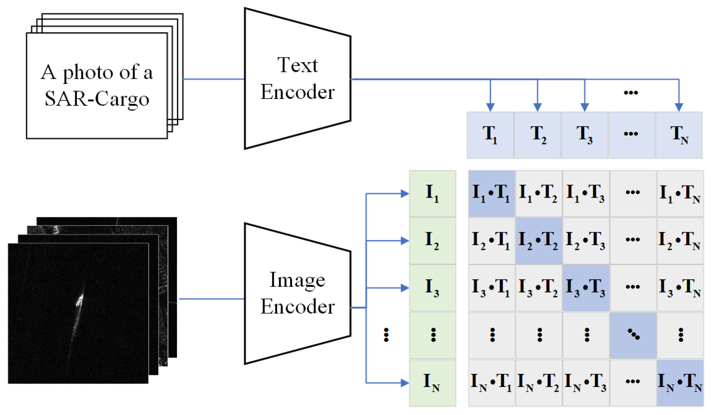
3.2. Contrastive Language–Image Pre-Training (CLIP)

Contrastive Language–Image Pre-training (CLIP) [37] is a transferable multimodal model trained through contrastive learning using text as a supervisory signal. Unlike other contrastive learning methods in the computer vision domain, such as MoCo [38] and Simclr [39], CLIP’s training data consist of text–image pairs. This unique training approach enables CLIP to identify the correlation between text and images. By pairing text descriptions with the corresponding images, CLIP learns how to embed representations for both text and images and measures the similarity between them by comparing their embedding vectors. Consequently, CLIP can achieve cross-modal transfer learning across various tasks and domains.
As illustrated in Figure 2, CLIP employs a Text Encoder and an Image Encoder. The former is employed to extract features from text and can use commonly available text Transformer models in NLP. The latter is responsible for extracting features from images and can use popular CNN models or ViT. The training process of CLIP on a text–image paired dataset can be described as follows. Firstly, if a batch in the dataset contains N text–image pairs, N texts are first encoded through the Text Encoder, assuming each text is encoded into a one-dimensional vector. The output of the Text Encoder for this batch of text data is denoted by [ T 1 , T 2 , , T N ] . Similarly, the N images are encoded through the Image Encoder, assuming each image is encoded into a one-dimensional vector. The output of the Image Encoder for this batch of image data is denoted by [ I 1 , I 2 , , I N ] .
Secondly, in the obtained [ T 1 , T 2 , , T N ] and [ I 1 , I 2 , , I N ] , the text–image pairs have a one-to-one correspondence: i.e., T 1 corresponds to I 1 , T 2 corresponds to I 2 , etc. These N corresponding pairs are denoted as positive samples, whereas the non-corresponding text–image pairs (i.e., T 1 does not correspond to I 2 , T N does not correspond to I N 1 ) are denoted as negative samples. Thus, in total, there exist N positive samples and N 2 N negative samples, which are used as positive and negative labels to train the Text Encoder and Image Encoder.
Finally, for any i , j [ 1 , N ] , the cosine similarity between T i and I j is calculated to quantify the correspondence between the corresponding text and image. A larger cosine similarity indicates a stronger correspondence between I i and T j , and vice versa. Therefore, by training the parameters of the encoder, the goal is to increase the denormalized cosine measure of N positive samples and, at the same time, to decrease the denormalized cosine measure of N 2 N negative samples. The objective is as follows:
L = min ( i = 1 N j = 1 N ( I i · T j ) i = 1 N ( I i · T i ) ) .
As depicted in Figure 2, this corresponds to maximizing the blue background along the diagonal and minimizing the other non-diagonal values.

4. Methods

The overall framework of the proposed method is illustrated in Figure 3. As a backbone network, T2T-ViT achieves good results without the need for a massive pre-training dataset. In cases of insufficient data samples, we employ an image generation module. In the Conditioning Module, text information is input and encoded, combined with the U-Net structure in the image generation module. This integration generates SAR ship images corresponding to the textual descriptions, serving as supplements. Subsequently, the data samples are input into the T2T-ViT network for training. Incorporating an SE attention mechanism into the backbone network enhances its focus on crucial features, optimizing overall performance. After processing through the T2T module, the input images are fed into the backbone network, ultimately yielding the classification results of the target.

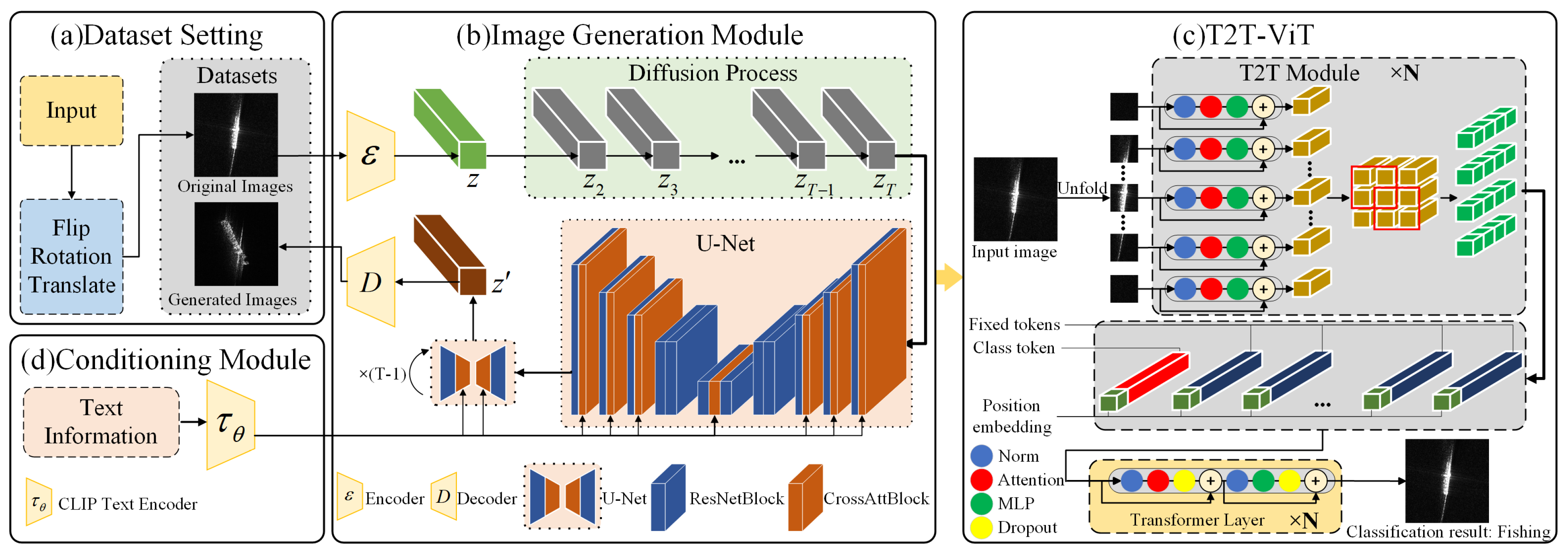
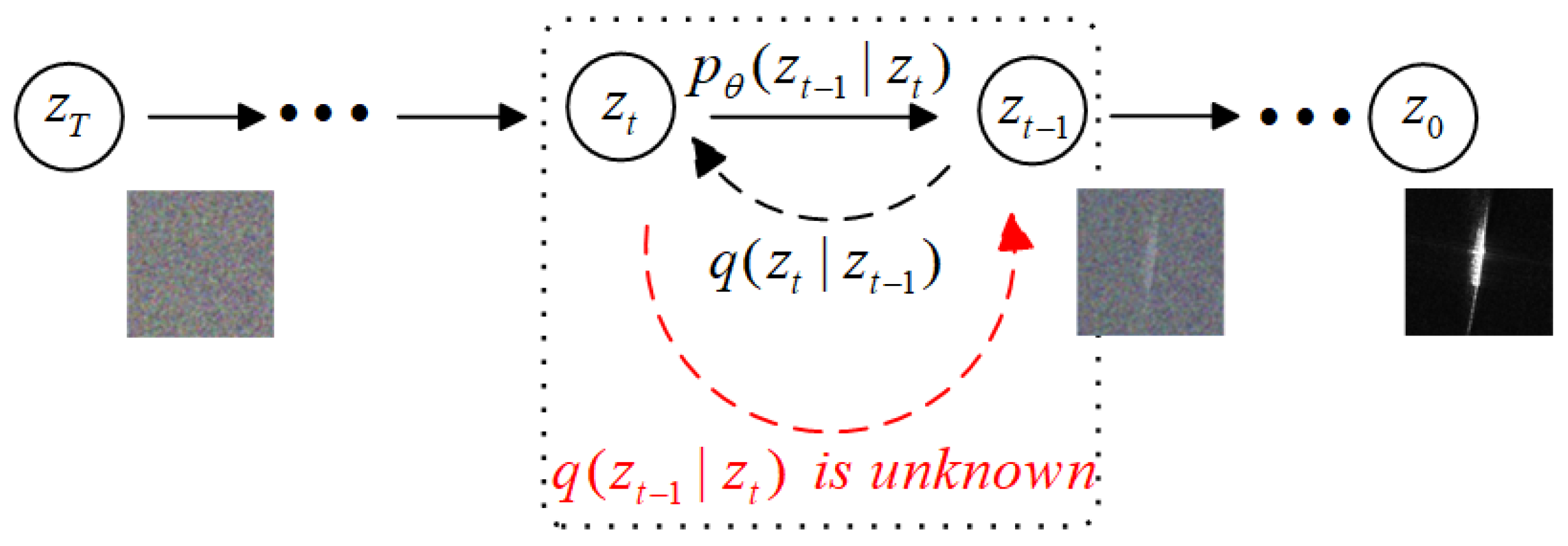
4.1. Image Generation Module

The introduction of the image generation module is based on the implementation of the LDM, and the operational structure is illustrated in Figure 3b. Firstly, it is necessary to have a variational autoencoder model comprising an encoder ϵ and a decoder D . We input the image into the encoder for compression processing, converting it from the pixel space to feature vectors within the latent space. This latent representation vector has a lower dimensionality, abstracting high-frequency and imperceptible details through dimensionality reduction. Next, a diffusion operation is performed on the latent representation space. This process occurs over continuous time steps, introducing Gaussian noise and gradually reducing the level of noise. Lastly, the decoder is employed to reconstruct the latent representation back into the pixel space. Its purpose is to transform vectors from the latent space into the high-dimensional pixel space, producing high-quality images that closely match the source image.
The handling of vectors in the latent space is akin to the function of the fundamental diffusion model (DM) [40]. The detailed operation of the DM is depicted in Figure 4. This model is based on a parameterized Markov chain and operates through two distinct procedures: the diffusion process and the denoising process.
The original input data are progressively mixed with Gaussian noise as part of the diffusion process, which will end after a predetermined number of iterations when these data become completely random. Gaussian noise is added at each stage of a diffusion process with T steps for the original input data z 0 q z 0 in the following manner:
q z t z t 1 = N z t ; 1 ψ t z t 1 , ψ t I ,
where ψ t is the variance of the noise added in step t, which increases with each step, i.e., ψ 1 < ψ 2 < < ψ T . As the step size T grows, the input image gradually loses all its original information and is transformed into random noise labeled as z T . The diffusion process involves adding noise iteratively, with the output at each step denoted by z t . This characteristic allows the diffusion process to be represented by a Markov process, which can be mathematically expressed as follows:
q z 1 : T z 0 = t = 1 T q z t z t 1 .
The denoising process occurs in a manner opposite to the previous process operation, during which we gradually remove noise from the data. If the function distribution q z t 1 z t can be obtained at each step of the denoising process, then the initial input image information can be extracted despite the presence of pure random noise z T N 0 , I by removing the noise repeatedly. Therefore, the denoising process can be considered a data generation process. In this process, the Gaussian distribution of each state is parameterized using neural networks and is correlated with the others in a Markov chain. This operation can be mathematically expressed as follows:
p θ z 0 : T = p z T t = 1 T p θ z t 1 z t ,
where p θ z t 1 z t = N z t 1 ; μ θ z t , t , Σ θ z t , t is a parameterized Gaussian distribution, and p z T N z T ; 0 , I . The core processing section of the DM, denoted by e θ ( o , t ) , is set as a time-conditioned U-Net, which utilizes 2D convolutional layers to build the lower-level U-Net’s ability, further focusing on the most relevant perceptual parts. The loss function, L D M , can be written as
L D M = E ε ( x ) , e ( 0 , 1 ) , t | | e e θ ( z t , t ) | | 2 2 .
In contrast to traditional diffusion models, we optimize the processing of input feature vectors in the previous U-Net by introducing a mechanism called cross-attention [41], transforming it into a more flexible conditional image generator. This method has shown good performance in handling models based on attention mechanisms that learn multiple input patterns. In order to combine different types of modalities (such as images or text descriptions) with the image generation module, an encoder corresponding to the input modality y is added, which we refer to as τ θ . The encoder can convert various modalities of input information into a feature vector τ θ ( y ) R M × d τ , which is then used as an input into the U-Net to combine with the latent features being denoised through cross-attention.
Based on image-conditioned inputs, the conditions can be obtained using the following expression:
L L D M = E ε ( x ) , y , e ( 0 , 1 ) , t | | e e θ ( z t , t , τ θ ( y ) ) | | 2 2 ,
where the optimization process involves jointly optimizing both τ θ and e θ . The structure of the Conditioning Module is illustrated in Figure 3d. This modulation mechanism offers versatility, as demonstrated in our study, where CLIP is utilized to generate images.

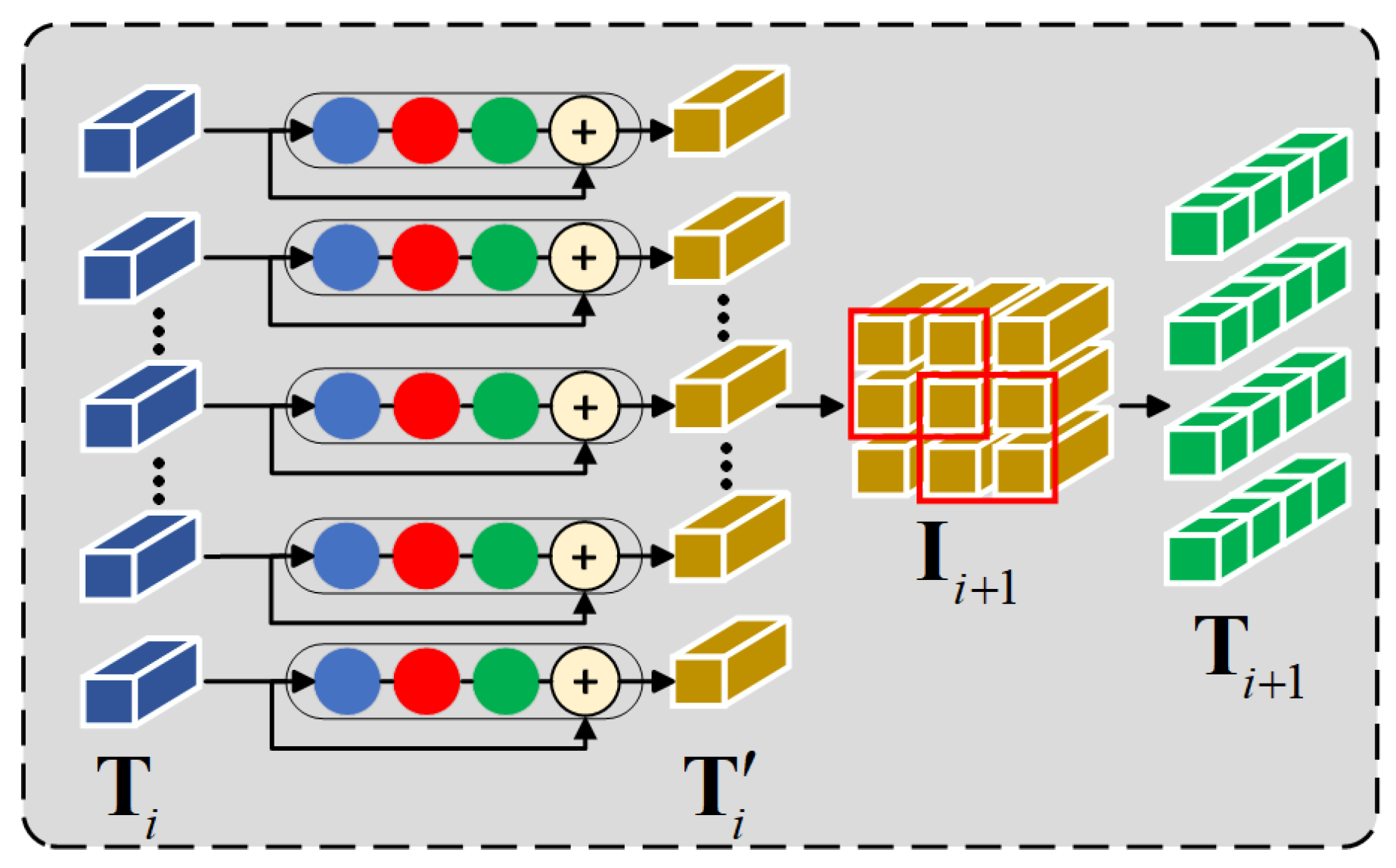
4.2. Tokens-to-Token Vision Transformers (T2T-ViT)

T2T-ViT [16] is a model for image processing that extracts image features and performs sequence modeling through two stages of processing. Its structure is illustrated in Figure 3c, and its operation will be described next. Initially, the image is divided into equally sized image blocks and encoded through a series of nested Transformer encoders to generate locally informed representations of the image. Subsequently, the obtained feature vectors containing local information are sent to the backbone network, resulting in a feature representation containing the overall information of the image. The model gradually converts the image into a token with an efficient backbone structure.
Its key component is the T2T module, which is purpose-built to capture and model the local structural information within the image. Additionally, this module facilitates a gradual reduction in the number of tokens as the image progresses. In this way, the T2T module can represent different regions and features of the image as relatively short token sequences, achieving the effective compression and expression of image information. The T2T module, as shown in Figure 5, performs two operations, namely, reconstruction and soft splitting.
The output token sequence, T i , is used as input into the T2T Transformer for processing, and T i is obtained through the following detailed operations, as described by
T i = MLP ( MSA ( T i ) ) .
MSA represents layer-normalized multi-head self-attention, the function of which is to capture dependencies at different positions in the sequence through multi-head attention calculations. Furthermore, MLP is a layer-normalized multilayer perceptron, which is used to process feature representations at each location. Then, these symbols are reshaped in the spatial dimension to form the image I i :
I i = Reshape ( T i ) ,
where Reshape rearranges tokens T R l × c into the image I R h × w × c , where l is the length of T , and h , w , c represent height, width, and the number of channels, respectively, satisfying l = h × w .
After obtaining the reconstructed image I i , the local structural information is modeled through soft splitting to reduce the number of tokens:
T i + 1 = SoftSplit ( I i ) , i = 1 , 2 , , ( n 1 ) .
The output tokens created during the current T2T process are then sent to the subsequent Transformer layer. In order to prevent information loss during token generation from reconstructed images, we adopt a strategy of segmenting SAR ship images into overlapping patches. This approach establishes prior knowledge by relating each patch to its neighboring patches, thereby promoting stronger correlations between tokens in close proximity. By connecting the tokens within each segmented patch together, local information can be effectively aggregated and is beneficial for subsequent processing.

4.3. Squeeze-and-Excitation (SE) Module

In ViT, the multi-head attention mechanism plays a vital role in the Transformer layer. This mechanism not only generates attention layer outputs with encoded representation information but also learns relationships between positions in the input sequence to better capture its intrinsic structure and semantic information. In the context of multi-head attention, the input sequence is first transformed into three distinct vectors: query, key, and value sequences. Subsequently, the similarity between each query vector and the key vectors is calculated, resulting in a weighting distribution for each query vector across all key vectors. Next, the obtained weight distribution is adapted to perform weighted averaging on the value vector, resulting in the output representation for each query vector. The multi-head attention repeats this procedure multiple times, each time using different projection matrices for queries, keys, and values to generate different attention subspaces. At the end, the final output is created by concatenating the results from each subspace and is used to perform subsequent operations.
The structure of the SE module is illustrated in Figure 6. In order to highlight the important features, the SE module has been added after the output of the multi-head attention mechanism. The SE module consists of squeeze and excitation components, reconstructing channel weights by modeling relationships between channels. Therefore, features related to channel regions become more prominent.
The essence of the squeeze operation is a pooling operation F s q ( · ) , which compresses the input feature map M by pooling, converting the spatial information contained in it into channel information A R N . The calculation of the l t h feature vector in A is as follows:
a l = F s q ( m l ) = 1 H × W i = 1 H j = 1 W m l ( i , j ) .
where A = [ a 1 , a 2 , , a l ] , M = [ m 1 , m 2 , , m l ] , where m l is the l t h feature vector corresponding to the input feature map. After obtaining the compressed feature information, an incentive function F e x ( · ) is used to extract the relationship B between channels, that is, the degree of attention to each channel, which can be computed as,
B = F e x ( A ) = σ ( V 2 δ ( V 1 A ) ) ,
where δ represents the ReLU activation function of the first fully connected layer, σ represents the sigmoid activation function of the second fully connected layer, and V 1 and V 2 represent the weight matrices of the fully connected layers.
The final output of the SE module is obtained by rescaling A through the activation B and is given by
C l = F s c a l e ( a l , b l ) = a l b l ,
where F s c a l e ( · ) represents reconstruction functions, and C = [ c 1 , c 2 , , c l ] represents the product of the obtained weights b l and the original feature map a l in the corresponding channels. During the task-learning process, the weights of channels related to the context are increased, enhancing the expressive power of features.

5. Experiments and Performance Evaluation Results

In the previous section, we propose an improved SAR ship classification method based on text-to-image generation and an SE module integrated with T2T-ViT. In this section, we will evaluate the performance of our proposed classification method against other conventional target classification techniques using two publicly available SAR ship datasets. We also present the results of ablation experiments and category expansion experiments to demonstrate the superiority of the proposed method.

5.1. Datasets and Settings

The OpenSARShip2.0 dataset is sourced from the Sentinel-1 satellite [42]. All images in the dataset were obtained in Interferometric Wide (IW) mode, covering nearly all global land and coastal areas. A notable feature of this dataset is the generation of ship labels using information obtained from an automated recognition system, providing the data labels with higher reliability. OpenSARShip2.0 comprises approximately 35,000 SAR ship images, including vessels from 14 categories, such as cargo ships, cruise ships, passenger ships, law enforcement vessels, and fishing boats. The resolution is 20 m × 20 m, with pixel sizes of 10 m × 10 m in the azimuth and range directions.
Three major categories with relatively abundant samples were initially selected from the OpenSARShip2.0 dataset, namely, Cargo, Fishing, and Tug, for our experiments. Figure 7 presents sample images of these three classes of SAR ships. However, it turned out that these original datasets have some drawbacks. Firstly, there is a lack of uniformity in the image sizes, which can be cumbersome for application to deep learning networks. Secondly, there is a significant disparity in the number of data samples among different ship categories, with Cargo having nearly 20,000 samples, far exceeding the sample counts of other ship categories. Therefore, we preprocessed the selected samples of the three ship categories by standardizing the image size to 224 × 224 pixels. Addressing the issue of class imbalance in the SAR ship dataset, data augmentation was performed on the training dataset. Initially, we applied horizontal and vertical flips to enhance the diversity of data samples. Subsequently, we rotated the data samples by 90°, 180°, and 270° to simulate various angles of vessels in real scenarios. Lastly, we randomly translated ship sample images, with pixel translation values ranging from −5 to 5, to introduce spatial variations in the data samples. Following a series of data augmentation processes, the data samples were expanded to four times their original size, as shown in Table 1, where the number of training samples for the three ship categories based on the OpenSARShip2.0 dataset can also be found.
The FUSAR-Ship dataset offers a comprehensive collection of high-resolution ship images. It comprises 15 primary ship categories and 98 subclasses, and it encompasses various marine targets, including objects other than ships [43]. The ship images in this dataset were obtained from China’s GF-3 satellite, which features a civilian C-band spaceborne SAR system. This advanced technology enables the satellite to capture SAR images with a high azimuth resolution of 1.124 m × 1.728 m and full-polarization capabilities. The imaging mode is the Ultra-Fine Stripmap mode, covering various scenes, such as sea, land, coastlines, rivers, and islands. Due to the extremely limited sample number of some ship categories in the FUSAR-Ship dataset, we selected the following five ship categories to further validate the effectiveness of our model: Bulk Carrier, Cargo, Fishing, Tanker, and Other. Figure 8 displays sample images of the five classes of SAR ships in the FUSAR-Ship dataset. Similarly, to obtain a balanced dataset, a series of data augmentation processes were applied to the selected samples of the three ship categories to meet the basic requirements for training for the target classification task. The number of training samples for the five ship categories based on the FUSAR-Ship dataset is presented in Table 2.
In our experiments, we trained the models with the same parameter settings. For both the OpenSARShip2.0 and FUSAR-Ship datasets, the input image size was fixed at 224 × 224 pixels for all training instances. The Stochastic Gradient Descent optimizer was employed [44], utilizing a weight decay parameter of 0.005 and a momentum parameter of 0.9. The proposed network model underwent training for a total of 2000 iterations. Due to limited GPU memory, the batch size was set to an empirical value of 8 to improve training efficiency. To mitigate any potential issues associated with gradient vanishing during training, a relatively low learning rate of 0.0005 was chosen. By employing such a learning rate, we could better control the training update pace of the network, thereby aiding in achieving stable performance for our approach.

5.2. Performance Evaluation Indices

The classification results can be categorized into four types: true positive (TP), true negative (TN), false positive (FP), and false negative (FN). TP indicates instances where the model correctly predicts positive samples as positive, TN denotes cases where the model correctly predicts negative samples as negative, FP represents instances where the model erroneously predicts negative samples as positive, and FN signifies cases where the model erroneously predicts positive samples as negative. Similar to previous studies [45,46,47,48], Accuracy is selected as the main evaluation metric to gauge the model’s performance in terms of classification to determine how effective the process suggested in this paper is. The percentage of correctly predicted samples out of the total is referred to as Accuracy, which is computed as follows:
Accuracy = TP + TN TP + TN + FP + FN .
Furthermore, three additional performance metrics were used in the experiments for further result validation: Precision, Recall, and F1 Score. Precision measures the percentage of true positive samples among the samples predicted by the model as positive. It provides insight into the correctness of the positive predictions and can be calculated as
Precision = TP TP + FP .
Recall, also known as the True Positive Rate or Sensitivity, represents the percentage of true positive samples among the actual positive samples. It is a measure that focuses on capturing all positive instances and is related to the original samples, and it is computed as
Recall = TP TP + FN .
F1 Score is a comprehensive metric that takes into account both Precision and Recall, providing a balanced measure of the model’s performance. It can be computed as
F 1 S c o r e = 2 × Precision × Recall Precision + Recall .
In order to effectively evaluate the generated images, we employed the Structure Similarity Index Measure (SSIM) [49], which is a metric for assessing the similarity between two images, taking into account information pertaining to luminance, contrast, and structure.
To assess the similarity between the mean brightness of two images, we define a luminance contrast function as follows:
I x , y = 2 μ x μ y + C 1 μ x 2 + μ y 2 + C 1 ,
where μ x and μ y represent the mean of the local blocks of images x and y. C 1 is a small constant used to stabilize the divisor, usually taking ( k 1 · M A X ) 2 , where M A X is the largest possible value of the pixel value, and k 1 is a small constant.
Considering the brightness variance and the covariance between the two images, the contrast function is defined by
C x , y = 2 σ x σ y + C 2 σ x 2 + σ y 2 + C 2 ,
where σ x and σ y represent the standard deviation of the local block of images x and y, σ x y is the covariance between x and y, C 2 is a small constant used to stabilize the divisor, usually ( k 2 · M A X ) 2 , and k 2 is a small constant.
The structural similarity is measured by the similarity between brightness and contrast, and we define the structural contrast function as follows:
S x , y = σ x y + C 3 σ x σ y + C 3 ,
where σ x and σ y represent the standard deviation of the local block of images x and y, σ x y is the covariance between x and y, and C 2 is a small constant used to stabilize the divisor, usually C 3 = C 2 / 2 .
Finally, the total SSIM is obtained by combining brightness similarity, contrast similarity, and structural similarity, and it is computed as follows:
S S I M x , y = I x , y α · C x , y β · S x , y γ ,
where α , β , and γ are used to adjust the importance between the three modules, usually taking a value of 1.

5.3. Image Generation Experiment

After incorporating the image generation module into the model, we expanded the imbalanced dataset of three selected categories from OpenSARShip2.0. Taking the existing samples of three ship categories as input, corresponding to the language texts SAR-Cargo, SAR-Fishing, and SAR-Tug, the model underwent iterative training. By providing textual information as input, the model generated corresponding SAR ship images. To verify the credibility of the generated images, the SSIMs between the generated images and the original dataset were calculated, and the average result obtained reached 0.837, which proves that we successfully captured the features of the SAR ship. Due to the limitation of training samples, generating SAR ship images is performed from a top-down perspective. Typical samples of various ship categories generated by the image generation module are shown in Figure 9.
From the above performance evaluation results, it can be concluded that the images generated by the image generation module meet the standards as a dataset, exhibiting high resolution and clarity. This indicates that these generated images can be used to train models or conduct other relevant research. By leveraging these generated images, we can more accurately capture and classify the features of the target objects, effectively improving the precision and efficiency of model training. This is clearly very important for further optimizing and enhancing ship classification algorithms. For the three selected ship categories in the OpenSARShip2.0 dataset, we successfully augmented the training set to 700 images using the generated image samples. This means that, in subsequent ship classification experiments, we have a more extensive and comprehensive dataset. By using such a dataset, we can more comprehensively evaluate and fine-tune our ship classification model to achieve even more accurate and reliable classification results.

5.4. Performance Comparison Results

To more comprehensively evaluate the effectiveness of the proposed method, we compared it with three traditional machine learning models and nine deep learning classification models on the OpenSARShip2.0 and FUSAR-Ship datasets. In terms of the number of network layers in the proposed method, we chose 14 Transformer layers, as this selection is the most appropriate choice for the best balance between model accuracy and model parameters. The traditional machine learning models include SVM [50], Adaboost [51], and KNN [52]. The deep learning models include LeNet [25], AlexNet [26], ResNet [30], MobileNet [31], DeiT [53], DenseNet [54], EfficientNet [55], Shufflenet [56], and CSPNet [57]. The comparison results are shown in Table 3.
From Table 3, it can be observed that our proposed method achieved higher classification performance compared to other classic deep learning target classification algorithms on the three categories of the OpenSARShip2.0 dataset. It achieved an Accuracy of 74.46 % , whereas the second-best algorithm, Shufflenet, achieved 73.41 % . There were also improvements in other evaluation metrics. When conducting five classification experiments on the FUSAR-Ship dataset, which is not limited to the classification of three types of ships, the increase in categories made classification more difficult. However, our proposed method still achieved the best classification performance, with an accuracy of 72.19 % , which is 0.83 % higher than the suboptimal algorithm Shufflenet. The other three evaluation indicators also showed some improvement, with 0.76 % , 0.91 % , and 0.63 % . The proposed method requires 53 s per epoch during training, which is mid-level compared to the other networks. When conducting image classification, the classification time for eight images in our proposed method is 51.37 ms, which is not significantly different from the inference time of most other models. In summary, in the face of imbalanced training samples, our proposed method demonstrated stronger capabilities by supplementing training samples through the image generation module and adjusting feature weights using the SE attention mechanism. Therefore, it is well suited for addressing data scarcity situations.

5.5. Performance Results

To verify the effectiveness of the image generation and SE modules in improving the performance, we conducted ablation experiments on three categories of the OpenSARShip2.0 ship dataset. Specifically, we compared the results of experiments with and without these two modules and calculated their respective classification accuracies. The results of the ablation experiments are shown in Table 4, where “✓” indicates the addition of these two modules to the base model T2T-ViT.
From the performance results presented in Table 4, it can be observed that T2T-ViT, as a variant model of ViT, outperforms ViT by better utilizing information in the image through the use of the T2T module, even without extensive pre-training on large datasets. This is consistent with the imbalance and lack of training data images faced in the classification of SAR ships. Thus, by using the T2T-ViT model as the backbone network and by also employing the proposed modules, the classification accuracy of the three categories of OpenSARShip2.0 ships was increased by 2.23 % , 1.46 % , and 3.55 % .
In addition, we used the image generation module as the main component and conducted more in-depth experiments to explore the effect of the generated data samples on the classification results. Initially, there were 558, 514, and 486 original training samples for the three types of ships. After using the image generation module, the number of training samples had expanded to 700. The results are shown in Table 5, where “×” indicates the absence of the image generation module in the base model, and “✓” indicates the presence of the image generation module in the base model.
These results reflect the advantage of using the image generation module on the classification performance of three ship categories. As seen in Table 5, it is also noted that the best classification performance is obtained for Cargo ships, which is due to their distinct characteristics, as they typically carry standard-sized containers. This unique structural feature, with a small-width deck edge, sets Cargo ships apart from other ship categories, making their features more evident in remote sensing images and facilitating clearer feature extraction during model training. It is clear that the use of the image generation module resulted in improvements in Precision, Recall, and F1 Score for all categories. For example, the F1 Score increased by 1.84 % , 8.75 % , and 3.08 % , respectively. This demonstrates that the enhancement provided by this module is reasonable, particularly in situations with limited data availability.

5.6. Expansion of Experiment to Four Categories

To further investigate the effectiveness of our proposed method, we conducted training on a fourth ship category, namely, Tanker, using the OpenSARShip2.0 dataset. We selected 250 valid images of oil tankers and 400 images of the other three categories of ships from the existing dataset. In comparison to the other three ship categories, this sample size was evidently insufficient to support effective classification training for the fourth ship category. Therefore, we employed the image generation module to augment the data to 400 images. Subsequently, we divided the data into training and testing sets at a 4:1 ratio and incorporated them into the improved T2T-ViT for training. The classification performance results for the four ship categories are presented in Table 6, where we used the basic model to train on the dataset with unbalanced samples. Due to the similarity between classes of SAR ship data, when training tankers with a small number of data samples, the basic model is unable to effectively extract features, resulting in the misdiagnosis of tankers as ships of other classes. The introduction of the image generation module not only successfully maintains the classification of the three basic ship categories but also improves the recognition rate of the fourth ship category, “Tanker”. In the overall evaluation of the model, the most important evaluation indicator, Accuracy, reveals a recognition rate of 59.03 % with the basic model due to the relatively small proportion of Tanker samples in the original data. The recognition rate of 60.26 % with the improved model clearly shows that it has been effectively improved.
Compared to training with only the original dataset, the application of the image generation module provides us with additional training samples, so this approach enables a more comprehensive SAR ship classification. The use of the image generation module effectively augments the dataset, providing the algorithm with richer sample information, thereby improving the network’s generalization ability and classification accuracy. This not only showcases the effectiveness of the image generation module in expanding the dataset but also confirms the feasibility and practicality of our proposed method. By incorporating the image generation module, our approach adapts better to various ship categories and achieves satisfactory classification results.

6. Conclusions

In our paper, a novel SAR ship classification method is proposed to address the issue of inter-class sample imbalance in the SAR ship dataset. The improved approach utilizes text-to-image generation to mitigate the imbalance in the dataset, addressing the deficiency of insufficient data samples by introducing deep image modules into T2T-ViT in a text-to-image manner. Simultaneously, the SE model is introduced to enhance the network’s focus on key features, thereby improving classification accuracy. Classification experiments were conducted on the OpenSARShip2.0 dataset and the FUSAR-Ship dataset, demonstrating that our proposed method outperforms other algorithms in Precision, Recall, F1 Score, and Accuracy. Additionally, we conducted ablation experiments and extended ship classification experiments with four categories, further proving the effectiveness and stability of the proposed method.

Author Contributions

Conceptualization, L.W. and C.Z.; methodology, L.W. and Y.Q.; software, Y.Q.; validation, L.W. and P.T.M.; formal analysis, C.Z.; data curation, S.M.; writing—original draft preparation, Y.Q. and L.W.; writing—review and editing, L.W. and P.T.M. All authors have read and agreed to the published version of the manuscript.

Funding

National Natural Science Foundation of China: 62301184 and 62371153.

Data Availability Statement

The images used in this paper come from OpenSARShip2.0 and FUSAR-Ship.

Conflicts of Interest

The authors declare no conflicts of interest.

References

  1. Elachi, C. Spaceborne Imaging Radar: Geologic and Oceanographic Applications. Science 1980, 209, 1073–1082. [Google Scholar] [CrossRef] [PubMed]
  2. Petit, M.; Stretta, J.M.; Farrugio, H.; Wadsworth, A. Synthetic Aperture Radar Imaging of Sea Surface Life and Fishing Activities. IEEE Trans. Geosci. Remote Sens. 1992, 30, 1085–1089. [Google Scholar] [CrossRef]
  3. Born, G.H.; Dunne, J.A.; Lame, D.B. Seasat Mission Overview. Science 1979, 204, 1405–1406. [Google Scholar] [CrossRef] [PubMed]
  4. Iervolino, P.; Guida, R. A Novel Ship Detector Based on the Generalized-Likelihood Ratio Test for SAR Imagery. IEEE J. Sel. Top. Appl. Earth Obs. Remote Sens. 2017, 10, 3616–3630. [Google Scholar] [CrossRef]
  5. Yang, H.; Cao, Z.; Cui, Z.; Pi, Y. Saliency Detection of Targets in Polarimetric SAR Images Based on Globally Weighted Perturbation Filters. ISPRS J. Photogramm. Remote Sens. 2019, 147, 65–79. [Google Scholar] [CrossRef]
  6. Xie, T.; Zhang, W.; Yang, L.; Wang, Q.; Huang, J.; Yuan, N. Inshore Ship Detection Based on Level Set Method and Visual Saliency for SAR Images. Sensors 2018, 18, 3877. [Google Scholar] [CrossRef] [PubMed]
  7. Margarit, G.; Tabasco, A. Ship Classification in Single-Pol SAR Images Based on Fuzzy Logic. IEEE Trans. Geosci. Remote Sens. 2011, 49, 3129–3138. [Google Scholar] [CrossRef]
  8. Lang, H.; Wu, S.; Xu, Y. Ship Classification in SAR Images Improved by AIS Knowledge Transfer. IEEE Geosci. Remote Sens. Lett. 2018, 15, 439–443. [Google Scholar] [CrossRef]
  9. Xu, Y.; Lang, H. Distribution Shift Metric Learning for Fine-Grained Ship Classification in SAR Images. IEEE J. Sel. Top. Appl. Earth Obs. Remote Sens. 2020, 13, 2276–2285. [Google Scholar] [CrossRef]
  10. Xuand, X.; Zhang, X.; Zhang, T. Multi-Scale SAR Ship Classification with Convolutional Neural Network. In Proceedings of the IEEE International Geoscience and Remote Sensing Symposium IGARSS, Brussels, Belgium, 11–16 July 2021. [Google Scholar]
  11. Bentes, C.; Velotto, D.; Tings, B. Ship Classification in TerraSAR-X Images with Convolutional Neural Networks. IEEE J. Ocean. Eng. 2018, 43, 258–266. [Google Scholar] [CrossRef]
  12. He, J.; Wang, Y.; Liu, H. Ship Classification in Medium-Resolution SAR Images via Densely Connected Triplet CNNs Integrating Fisher Discrimination Regularized Metric Learning. IEEE Trans. Geosci. Remote Sens. 2021, 59, 3022–3039. [Google Scholar] [CrossRef]
  13. Sun, Y.; Wang, Z.; Sun, X.; Fu, K. SPAN: Strong Scattering Point Aware Network for Ship Detection and Classification in Large-Scale SAR Imagery. IEEE J. Sel. Top. Appl. Earth Obs. Remote Sens. 2022, 15, 1188–1204. [Google Scholar] [CrossRef]
  14. Shang, Y.; Pu, W.; Wu, C.; Liao, D.; Xu, X.; Wang, C.; Huang, Y.; Zhang, Y.; Wu, J.; Yang, J.; et al. HDSS-Net: A Novel Hierarchically Designed Network with Spherical Space Classifier for Ship Recognition in SAR Images. IEEE Trans. Geosci. Remote Sens. 2023, 61, 5222420. [Google Scholar] [CrossRef]
  15. Rombach, R.; Blattmann, A.; Lorenz, D.; Esser, P.; Ommer, B. High-Resolution Image Synthesis with Latent Diffusion Models. In Proceedings of the IEEE/CVF Conference on Computer Vision and Pattern Recognition (CVPR), New Orleans, LA, USA, 18–24 June 2022. [Google Scholar]
  16. Yuan, L.; Chen, Y.; Wang, T.; Yu, W.; Shi, Y.; Jiang, Z.; Tay, F.E.H.; Feng, J.; Yan, S. Tokens-to-Token ViT: Training Vision Transformers from Scratch on ImageNet. In Proceedings of the IEEE/CVF International Conference on Computer Vision (ICCV), Montreal, BC, Canada, 11–17 October 2021. [Google Scholar]
  17. Hu, J.; Shen, L.; Sun, G. Squeeze-and-Excitation Networks. In Proceedings of the IEEE/CVF Conference on Computer Vision and Pattern Recognition, Salt Lake City, UT, USA, 18–23 June 2018. [Google Scholar]
  18. Gouaillier, V.; Gagnon, L. Ship Silhouette Recognition Using Principal Components Analysis. In Applications of Digital Image Processing XX; Tescher, A.G., Ed.; SPIE: Bellingham, WA, USA, 1997. [Google Scholar]
  19. Wang, B.; Binford, T.O. Generic, Model-Based Estimation and Detection of Peaks in Image Surfaces; Association for Computing Machinery: New York, NY, USA, 1996. [Google Scholar]
  20. Touzi, R.; Raney, R.K.; Charbonneau, F. On the Use of Permanent Symmetric Scatterers for Ship Characterization. IEEE Trans. Geosci. Remote Sens. 2004, 42, 2039–2045. [Google Scholar] [CrossRef]
  21. Margarit, G.; Mallorqui, J.J.; Fabregas, X. Single-Pass Polarimetric SAR Interferometry for Vessel Classification. IEEE Trans. Geosci. Remote Sens. 2007, 45, 3494–3502. [Google Scholar] [CrossRef]
  22. Wang, J.; Xu, Y.; Zhang, X. The Active Appearance Model with Applications to SAR Target Recognition; Academy Publisher: Guwahati, India, 2009. [Google Scholar]
  23. Knapskog, A.O. Classification of Ships in TerraSAR-X Images Based on 3D Models and Silhouette Matching. In Proceedings of the European Conference on Synthetic Aperture Radar, Aachen, Germany, 7–10 June 2010; pp. 1–4. [Google Scholar]
  24. Chen, W.; Ji, K.; Xing, X.; Zou, H.; Sun, H. Ship Recognition in High Resolution SAR Imagery Based on Feature Selection. In Proceedings of the International Conference on Computer Vision in Remote Sensing, Xiamen, China, 16–18 December 2012. [Google Scholar]
  25. Lecun, Y.; Bottou, L.; Bengio, Y.; Haffner, P. Gradient-Based Learning Applied to Document Recognition. Proc. IEEE 1998, 86, 2278–2324. [Google Scholar] [CrossRef]
  26. Krizhevsky, A.; Sutskever, I.; Hinton, G.E. ImageNet Classification with Deep Convolutional Neural Networks. Commun. ACM 2017, 60, 84–90. [Google Scholar] [CrossRef]
  27. Simonyan, K.; Zisserman, A. Very Deep Convolutional Networks for Large-Scale Image Recognition. arXiv 2014, arXiv:1409.1556. [Google Scholar]
  28. Lin, M.; Chen, Q.; Yan, S. Network in Network. arXiv 2013, arXiv:1312.4400. [Google Scholar]
  29. Szegedy, C.; Liu, W.; Jia, Y.; Sermanet, P.; Reed, S.; Anguelov, D.; Erhan, D.; Vanhoucke, V.; Rabinovich, A. Going Deeper with Convolutions. In Proceedings of the IEEE Conference on Computer Vision and Pattern Recognition (CVPR), Boston, MA, USA, 7–12 June 2015. [Google Scholar]
  30. He, K.; Zhang, X.; Ren, S.; Sun, J. Deep Residual Learning for Image Recognition. In Proceedings of the IEEE Conference on Computer Vision and Pattern Recognition (CVPR), Las Vegas, NV, USA, 27–30 June 2016. [Google Scholar]
  31. Howard, A.G.; Zhu, M.; Chen, B.; Kalenichenko, D.; Wang, W.; Weyand, T.; Andreetto, M.; Adam, H. MobileNets: Efficient Convolutional Neural Networks for Mobile Vision Applications. arXiv 2017, arXiv:1704.04861. [Google Scholar]
  32. Tan, M.; Chen, B.; Pang, R.; Vasudevan, V.; Sandler, M.; Howard, A.; Le, Q.V. MnasNet: Platform-Aware Neural Architecture Search for Mobile. In Proceedings of the IEEE/CVF Conference on Computer Vision and Pattern Recognition (CVPR), Long Beach, CA, USA, 15–20 June 2019. [Google Scholar]
  33. Wang, J.; Sun, K.; Cheng, T.; Jiang, B.; Deng, C.; Zhao, Y.; Liu, D.; Mu, Y.; Tan, M.; Wang, X.; et al. Deep High-Resolution Representation Learning for Visual Recognition. IEEE Trans. Pattern Anal. Mach. Intell. 2021, 43, 3349–3364. [Google Scholar] [CrossRef] [PubMed]
  34. Yu, C.; Xiao, B.; Gao, C.; Yuan, L.; Zhang, L.; Sang, N.; Wang, J. Lite-HRNet: A Lightweight High-Resolution Network. In Proceedings of the IEEE/CVF Conference on Computer Vision and Pattern Recognition (CVPR), Nashville, TN, USA, 20–25 June 2021. [Google Scholar]
  35. Vaswani, A.; Shazeer, N.; Parmar, N.; Uszkoreit, J.; Jones, L.; Gomez, A.N.; Kaiser, L.; Polosukhin, I. Attention Is All You Need. Adv. Neural Inf. Process. Syst. 2017, 30. Available online: https://proceedings.neurips.cc/paper_files/paper/2017/hash/3f5ee243547dee91fbd053c1c4a845aa-Abstract.html (accessed on 27 January 2024).
  36. Dosovitskiy, A.; Beyer, L.; Kolesnikov, A.; Weissenborn, D.; Houlsby, N. An Image is Worth 16x16 Words: Transformers for Image Recognition at Scale. arXiv 2020, arXiv:2010.11929. [Google Scholar]
  37. Radford, A.; Kim, J.W.; Hallacy, C.; Ramesh, A.; Goh, G.; Agarwal, S.; Sastry, G.; Askell, A.; Mishkin, P.; Clark, J. Learning Transferable Visual Models from Natural Language Supervision. In Proceedings of the International Conference on Machine Learning, Virtual, 18–24 July 2021. [Google Scholar]
  38. He, K.; Fan, H.; Wu, Y.; Xie, S.; Girshick, R. Momentum Contrast for Unsupervised Visual Representation Learning. In Proceedings of the IEEE/CVF Conference on Computer Vision and Pattern Recognition (CVPR), Seattle, WA, USA, 13–19 June 2020. [Google Scholar]
  39. Chen, T.; Kornblith, S.; Norouzi, M.; Hinton, G. A Simple Framework for Contrastive Learning of Visual Representations. In Proceedings of the International Conference on Machine Learning, Virtual, 13–18 July 2020. [Google Scholar]
  40. Ho, J.; Jain, A.; Abbeel, P. Denoising Diffusion Probabilistic Models. Adv. Neural Inf. Process. Syst. 2020, 33, 6840–6851. [Google Scholar]
  41. Mozhdeh, G.; Xiang, R.; Jonathan, M. Cross-Attention is All You Need: Adapting Pretrained Transformers for Machine Translation. arXiv 2021, arXiv:2104.08771. [Google Scholar]
  42. Li, B.; Liu, B.; Huang, L.; Guo, W.; Zhang, Z.; Yu, W. OpenSARShip 2.0: A Large-Volume Dataset for Deeper Interpretation of Ship Targets in Sentinel-1 Imagery. In Proceedings of the SAR in Big Data Era: Models, Methods and Applications (BIGSARDATA), Beijing, China, 13–14 November 2017. [Google Scholar]
  43. Hou, X.; Ao, W.; Song, Q.; Lai, J.; Wang, H.; Xu, F. FUSAR-Ship: Building A High-Resolution SAR-AIS Matchup Dataset of Gaofen-3 for Ship Detection and Recognition. Sci. China Inf. Sci. 2020, 63, 140303. [Google Scholar] [CrossRef]
  44. Theodoridis, S. Stochastic Gradient Descent; Elsevier: Amsterdam, The Netherlands, 2015. [Google Scholar]
  45. Zheng, H.; Hu, Z.; Yang, L.; Xu, A.; Zheng, M.; Zhang, C.; Li, K. Multifeature Collaborative Fusion Network with Deep Supervision for SAR Ship Classification. IEEE Trans. Geosci. Remote Sens. 2023, 61, 5212614. [Google Scholar] [CrossRef]
  46. Xu, Y.; Lang, H. Ship Classification in SAR Images with Geometric Transfer Metric Learning. IEEE Trans. Geosci. Remote Sens. 2021, 59, 6799–6813. [Google Scholar] [CrossRef]
  47. Lang, H.; Wu, S. Ship Classification in Moderate-Resolution SAR Image by Naive Geometric Features-Combined Multiple Kernel Learning. IEEE Geosci. Remote Sens. Lett. 2017, 14, 1765–1769. [Google Scholar] [CrossRef]
  48. Salerno, E. Using Low-Resolution SAR Scattering Features for Ship Classification. IEEE Geosci. Remote Sens. Lett. 2022, 19, 4509504. [Google Scholar] [CrossRef]
  49. Wang, Z.; Bovik, A.C.; Sheikh, H.R.; Simoncelli, E.P. Image Quality Assessment: From Error Visibility to Structural Similarity. IEEE Trans. Image Process. 2004, 13, 600–612. [Google Scholar] [CrossRef] [PubMed]
  50. Hearst, M.A.; Dumais, S.T.; Osuna, E.; Platt, J.; Scholkopf, B. Support Vector Machines. IEEE Intell. Syst. Their Appl. 1998, 13, 18–28. [Google Scholar] [CrossRef]
  51. Freund, Y.; Schapire, R.E. A Desicion-Theoretic Generalization of on-Line Learning and an Application to Boosting. In Proceedings of the Computational Learning Theory, Santa Cruz, CA, USA, 5–8 July 1995. [Google Scholar]
  52. Cover, T.; Hart, P. Nearest Neighbor Pattern Classification. IEEE Trans. Inf. Theory 1967, 13, 21–27. [Google Scholar] [CrossRef]
  53. Touvron, H.; Cord, M.; Douze, M.; Massa, F.; Sablayrolles, A.; Jégou, H. Training Data-Efficient Image Transformers Distillation through Attention. In Proceedings of the 38th International Conference on Machine Learning, Virtual, 18–24 July 2021. [Google Scholar]
  54. Huang, G.; Liu, Z.; Maaten, L.V.D.; Weinberger, K.Q. Densely Connected Convolutional Networks. In Proceedings of the IEEE Conference on Computer Vision and Pattern Recognition (CVPR), Honolulu, HI, USA, 21–26 July 2017. [Google Scholar]
  55. Tan, M.; Le, Q.V. EfficientNet: Rethinking Model Scaling for Convolutional Neural Networks. In Proceedings of the International Conference on Machine Learning, Long Beach, CA, USA, 10–15 June 2019. [Google Scholar]
  56. Zhang, X.; Zhou, X.; Lin, M.; Sun, J. ShuffleNet: An Extremely Efficient Convolutional Neural Network for Mobile Devices. In Proceedings of the IEEE/CVF Conference on Computer Vision and Pattern Recognition (CVPR), Salt Lake City, UT, USA, 18–23 June 2018. [Google Scholar]
  57. Wang, C.; Liao, H.M.; Wu, Y.; Chen, P.; Hsieh, J.; Yeh, I. CSPNet: A New Backbone that can Enhance Learning Capability of CNN. In Proceedings of the IEEE/CVF Conference on Computer Vision and Pattern Recognition Workshops (CVPRW), Seattle, WA, USA, 14–19 June 2020. [Google Scholar]
Figure 1. A structural comparison diagram between CNN and ViT.
Remotesensing 16 01299 g001
Figure 2. The pre-training process of CLIP.
Remotesensing 16 01299 g002
Figure 3. The overall framework of the proposed method.
Remotesensing 16 01299 g003
Figure 4. The operation of the diffusion model.
Remotesensing 16 01299 g004
Figure 5. The structure of the T2T module.
Remotesensing 16 01299 g005
Figure 6. The structure of the SE module.
Remotesensing 16 01299 g006
Figure 7. SAR ship samples from the OpenSARShip2.0 dataset representing (a) an optical image of Cargo; (b) a SAR image of Cargo; (c) an optical image of Fishing; (d) a SAR image of Fishing; (e) an optical image of Tug; and (f) a SAR image of Tug.
Remotesensing 16 01299 g007
Figure 8. SAR ship samples in FUSAR-Ship dataset. Among these, (ae) represent optical images of Bulk Carrier, Cargo, Fishing, Tanker, and Other, and (fj) represent SAR images of Bulk Carrier, Cargo, Fishing, Tanker, and Other.
Remotesensing 16 01299 g008
Figure 9. Image results generated by inputting text information: SAR Cargo, SAR Fishing, SAR Tug; (ac) represent Cargo images, while (df) represent Fishing images, and (gi) represent Tug images.
Remotesensing 16 01299 g009
Table 1. Three ship categories’ sample statistics from the FUSAR-Ship dataset.
CategoryTrainingTestingTotal
Cargo558178736
Fishing514178692
Tug486178664
Table 2. Five ship categories’ sample statistics from the FUSAR-Ship dataset.
CategoryTrainingTestingTotal
Bulk Carrier7224811203
Cargo7294861215
Fishing7264841210
Tanker7264831209
Other Ship7845221306
Table 3. A comparison of quantitative evaluation indicators on two datasets. For a clear display, the highest score in each column is highlighted in bold. Train time represents the time it takes for the model to train one epoch, and test time represents the time it takes for the model to classify 8 images at once.
MethodsOpenSARShip2.0 DatasetFUSAR-Ship DatasetSpeed
Precision (%)Recall (%)F1 Score (%)Accuracy (%)Precision (%)Recall (%)F1 Score (%)Accuracy (%)Train Time (s)Test Time (ms)
SVM [50]58.0257.8958.4758.2456.1256.4556.7356.36-29.45
Adaboost [51]49.7349.5249.2749.6439.9240.2740.3140.28-21.57
KNN [52]63.0162.8663.3263.0552.9552.6252.7152.87-14.82
LeNet [25]68.7267.8566.8468.0960.8760.2360.4160.21716.29
AlexNet [26]67.1266.6366.4166.4961.6562.0361.2262.182239.08
ResNet [30]59.2158.4058.0959.0460.4161.2760.8061.4160127.03
MobileNet [31]67.1167.5766.4367.5567.4167.0567.2767.132542.35
DeiT [53]57.6556.9455.9257.0952.9753.0451.8953.016861.89
DenseNet [54]67.1766.4966.5466.4867.8168.9668.0569.227448.56
EfficientNet [55]71.5271.7371.3272.1670.5970.4370.2770.693729.32
Shufflenet [56]73.5873.4173.1273.4171.2971.2171.3471.362645.60
CSPNet [57]70.0870.4969.4069.8870.4070.2370.2870.589442.34
Proposed method 74.13 73.96 73.94 74.46 72.05 72.12 71.97 72.19 5351.37
Table 4. Ablation experiments on three categories of OpenSARShip2.0 ship dataset.
BackboneImage Generation ModuleSE ModuleAccuracy (%)
ViT 64.89
T2T-ViT 72.13
T2T-ViT 74.02
T2T-ViT 73.59
T2T-ViT74.46
Table 5. The classification results of three categories of ships with the added image generation module on the OpenSARShip2.0 dataset.
Image Generation ModuleCategoryPrecision (%)Recall (%)F1 Score (%)
×Cargo79.5479.8179.67
Fishing68.4260.9464.46
Tug66.1872.5869.23
Cargo79.7982.2581.01
Fishing72.9465.4268.98
Tug69.6674.1971.85
Table 6. Classification results after adding a fourth category of ships from the OpenSARShip2.0 dataset.
MethodCategoryPrecision (%)Recall     (%)F1 Score (%)Accuracy (%)
T2T-ViTCargo67.1860.7963.8359.03
Fishing56.8363.9260.17
Tug58.3250.3254.03
Tanker54.4657.5255.95
Proposed methodCargo68.0661.2564.4760.26
Fishing57.1465.0360.82
Tug59.2651.6155.17
Tanker57.6561.2559.39
Disclaimer/Publisher’s Note: The statements, opinions and data contained in all publications are solely those of the individual author(s) and contributor(s) and not of MDPI and/or the editor(s). MDPI and/or the editor(s) disclaim responsibility for any injury to people or property resulting from any ideas, methods, instructions or products referred to in the content.

