Communication

Separation of Rapidly-Varying and Slowly-Varying Processes and Development of Diffraction Decomposition Order Method in Radiative Transfer

1
Department of Atmospheric and Oceanic Sciences, Fudan University, Shanghai 200438, China
2
CMA-FDU Joint Laboratory of Marine Meteorology, Shanghai 200438, China
3
Shanghai Key Laboratory of Ocean-Land-Atmosphere Boundary Dynamics and Climate Change, Shanghai 200438, China
*
Author to whom correspondence should be addressed.
These authors contributed equally to this work.
Remote Sens. 2024, 16(7), 1300; https://doi.org/10.3390/rs16071300
Submission received: 12 March 2024 / Revised: 30 March 2024 / Accepted: 3 April 2024 / Published: 7 April 2024

Abstract

:
Single scattering in radiative transfer is separated into rapidly-varying and slowly-varying processes, where the rapidly-varying process (RVP) is mainly contributed by the diffraction effect. Accordingly, the diffraction decomposition order (DDO) method is developed to solve the vector radiative transfer equation (VRTE). Instead of directly solving the original VRTE, we decompose it into a series of order equations, where the zeroth-order equation replaces the RVP with a δ -function while the high-order equations are the same as the zeroth-order one, except that the high decomposition orders of the RVP are used as driven sources. In this study, the DDO method is numerically realized using the successive order of the scattering method. The DDO is computationally efficient and accurate. More importantly, all physical processes in the VRTE are fully decomposed due to the order decomposition of the RVP and can be straightforwardly discussed.

1. Introduction

The radiative transfer process of electromagnetic energy is significant in atmospheric science, and is managed by the vector radiative transfer equation (VRTE) [1,2,3]. Many algorithms are developed to effectively solve the VRTE, such as the Discrete-Ordinate, adding-doubling, successive order of scattering, and Monte Carlo methods [4]. The radiative transfer methods are comprehensively discussed, and also compared to generate benchmark results (e.g., [5]).
Multiple scattering is an important process in radiative transfer. Scattering distribution in every scattering has a strong but steep forward peak due to the diffraction effect [6,7,8]. Direct calculation of the VRTE is usually time-consuming due to the strong diffraction peak. As a result, truncation techniques are developed to promote computational efficiencies, such as δ -M, δ -fit, and small-angle approximation methods [9,10,11]. Even though computational efficiency is significantly improved, computational accuracy is reduced due to the truncation with respect to the diffraction peak (e.g., [12,13,14]).
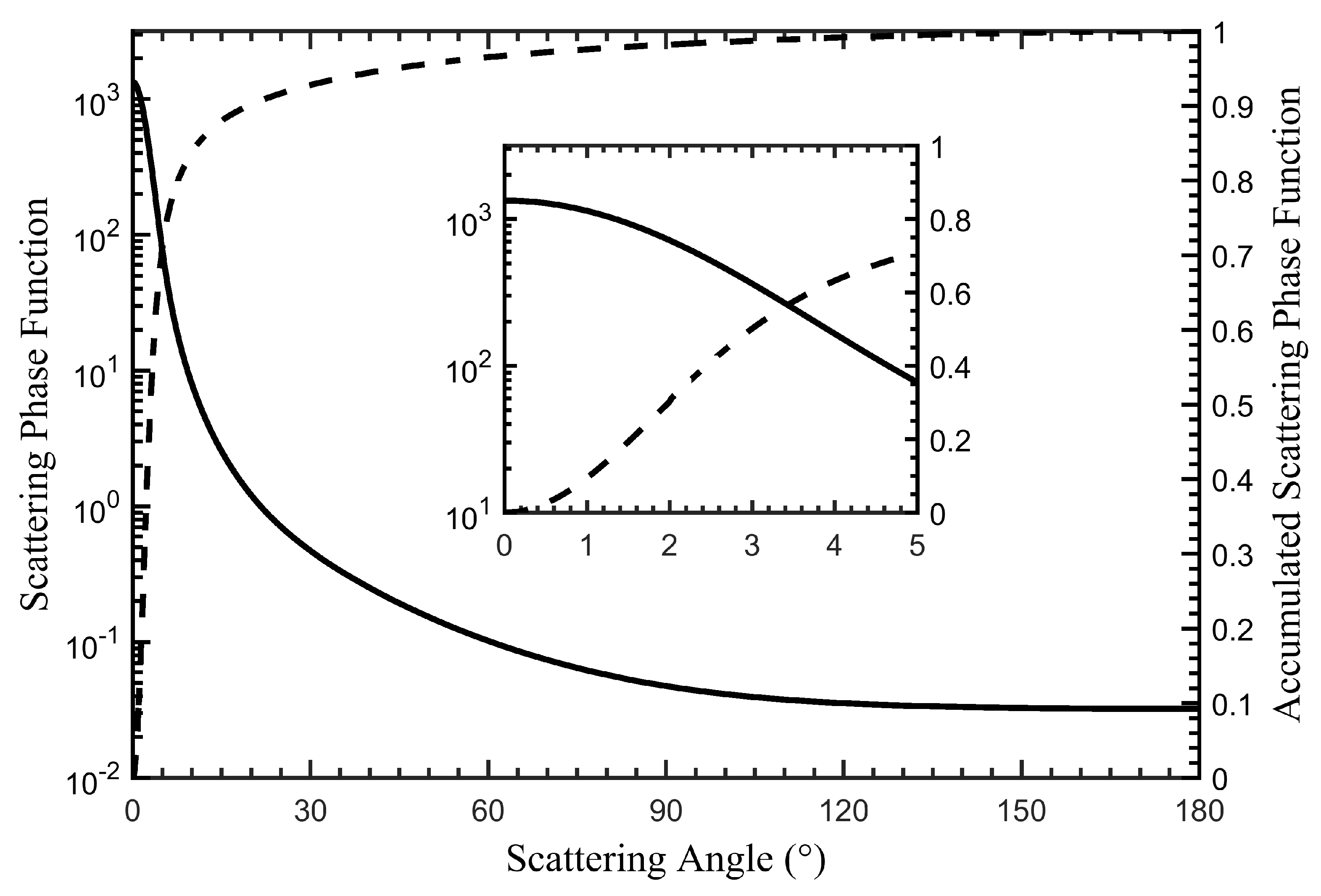
Other than diffraction, the ordinary scattering in every scattering is a slowly-varying process. Although the diffraction peak accounts for a large percentage of scattering energy, it is limited to narrow scattering angles and a rapidly-varying process, where an exemplary scattering phase function is shown in Figure 1. Based on the recognition, the diffraction peak can be decomposed into an order expansion, where the zeroth-order term is a δ -function and the high-order terms are associated with the high-order differences between the diffraction peak and the δ -function. Consequently, the original VRTE is decomposed into a series of order equations, called the diffraction decomposition order method (DDO). The rapidly-varying process is separated from the single scattering process and acts as driven sources for the high-order equations in the DDO method. The DDO method is efficient due to the direct δ -function replacement of the diffraction peak at the zeroth-order equation and accurate due to the successive consideration of the diffraction peak at the high-order equations. Moreover, the processes of successive order of scattering and diffraction decomposition are both reflected and discussed in this study.

2. Method

Only the radiative transfer process in the solar radiation is considered since the diffraction peak is weakened in the longwave radiation. Defining u = cos θ and μ = | u | , the VRTE in the plane-parallel assumption can be written as
u I ( Ω ) τ = I ( Ω ) ω 4 π 4 π P ( Ω , Ω ) I ( Ω ) d Ω ,
and the boundary condition at the top of the atmosphere is
I ( τ = 0 ; Ω ) = E 0 δ ( Ω Ω 0 ) , E 0 = F 0 / μ 0 0 0 0 T ,
where Ω and Ω 0 denote the viewing ( u , φ ) and solar ( μ 0 , φ 0 ) solid angles, respectively; d Ω = d u d φ ; δ ( Ω Ω 0 ) = δ ( u + μ 0 ) δ ( φ φ 0 ) ; I , P , and ω are the Stokes vector, scattering phase matrix, and single scattering albedo, respectively; F 0 is the solar irradiance. The argument τ  of the physical quantities is suppressed in the equations. Ω u and Ω d are used to denote the upward ( μ , φ ) and downward ( μ , φ ) solid angles.
In the DDO method, the scattering phase matrix P can be separated into the rapidly-varying process (RVP) (denoted by subscript ‘r’) and the slowly-varying process (SVP) (denoted by subscript ‘s’) as
P = f P r + ( 1 f ) P s ,
where f is the proportion factor of the RVP, and is usually a predefined parameter. We define the difference symbol between the RVP and the δ -function as
P r δ = P r 4 π Diag ( 1 , 1 , 1 , 1 ) δ ( Ω Ω ) .
Equation (1) is reduced into the zeroth-order equation only associated with the SVP when P r δ = 0 as
u I 0 ( Ω ) τ e = I 0 ( Ω ) ω e 4 π 4 π P s ( Ω , Ω ) I 0 ( Ω ) d Ω , I 0 ( τ e = 0 ; Ω ) = E 0 δ ( Ω Ω 0 ) ,
where the effective optical depth and single scattering albedo are defined as
τ e = ( 1 ω f ) τ , ω e = ω ( 1 f ) 1 ω f .
The residual equation of Equation (1) after the zeroth-order reduction is
u I r e s ( Ω ) τ = I r e s ( Ω ) ω 4 π 4 π P ( Ω , Ω ) I r e s ( Ω ) d Ω ω f 4 π 4 π P r δ ( Ω , Ω ) I 0 ( Ω ) d Ω .
Repeating the same operations as Equation (1) reduced to Equations (5)–(7), Equation (7) is successively decomposed into a series of order equations, as follows:
u I i ( Ω ) τ e = I i ( Ω ) ω e 4 π 4 π P s ( Ω , Ω ) I i ( Ω ) d Ω ω r 4 π 4 π P r δ ( Ω , Ω ) I i 1 ( Ω ) d Ω ,
where i = 1 , , , and the single scattering albedo associated with the RVP is
ω r = ω f 1 ω f .
The solution of Equation (5) is physically composed of direct and diffuse terms
I 0 = I 0 , d i r + I 0 , d i f = exp τ e μ 0 E 0 δ ( Ω Ω 0 ) + I 0 , d i f .
Substituting Equation (10) into Equation (5), the zeroth-order equation is simplified as
u I 0 , d i f ( Ω ) τ e = I 0 , d i f ( Ω ) ω e 4 π 4 π P s ( Ω , Ω ) I 0 , d i f ( Ω ) d Ω ω e 4 π exp τ e μ 0 P s ( Ω , Ω 0 ) E 0 .
For consistency, the notation I 0 is used to replace the diffuse term I 0 , d i f hereafter.
Substituting Equation (10) into Equation (8) at i = 1 , Equations (8), (10) and (11) can be consistently organized as follows:
u I i ( Ω ) τ e = I i ( Ω ) ω e 4 π 4 π P s ( Ω , Ω ) I i ( Ω ) d Ω S i ( Ω ) ,
where i = 0 , , , and the driven source functions S i are explicitly represented as
S 0 ( Ω ) = ω e 4 π exp τ e μ 0 P s ( Ω , Ω 0 ) E 0 , S 1 ( Ω ) = ω r 4 π 4 π P r δ ( Ω , Ω ) I 0 ( Ω ) d Ω + S 1 δ ( Ω ) , S i ( Ω ) = ω r 4 π 4 π P r δ ( Ω , Ω ) I i 1 ( Ω ) d Ω , i = 2 , , , S 1 δ ( Ω ) = ω r 4 π exp τ μ 0 P r ( Ω , Ω 0 ) E 0 , ω e 4 π exp τ e μ 0 exp τ μ 0 P s ( Ω , Ω 0 ) E 0 ,
and the corresponding direct term is
I d i r = exp τ μ 0 E 0 δ ( Ω Ω 0 ) .
The solution of the VRTE in Equation (1) can be obtained by
I = I d i r + i = 0 I i .
The source function S 1 δ in the first-order equation is explicitly from the direct term of the zeroth-order equation of Equation (10). It is reduced to a δ -function if the RVP is reduced to a δ -function, that is, when P r δ = 0 , S 1 δ = exp τ e / μ 0 exp τ / μ 0 E 0 δ ( Ω Ω 0 ) , which is exactly the direct term difference between Equations (10) and (15). The RVP stays in the driven source functions of the high-order equations while the SVP is involved in the multiple scattering processes, and the two processes are fully separated. The contribution of the diffraction effect is successively considered in the high-order equations. Equations (12)–(15) are the specific expressions of the DDO method.
The total optical depth is denoted as b and the effective total optical depth is b e = ( 1 ω f ) b , as in Equation (6). Formally, Equation (12) can be written as upward and downward components:
I i ( τ e ; Ω u ) = Γ μ τ e , b e I i ( b e ; Ω u ) + τ e b e d τ e μ Γ μ τ e , τ e ω e 4 π 4 π d Ω P s ( τ e ; Ω u , Ω ) I i ( τ e ; Ω ) + τ e b e d τ e μ Γ μ τ e , τ e S i ( τ e ; Ω u ) ,
I i ( τ e ; Ω d ) = Γ μ 0 , τ e I i ( 0 ; Ω d ) + 0 τ e d τ e μ Γ μ τ e , τ e ω e 4 π 4 π d Ω P s ( τ e ; Ω d , Ω ) I i ( τ e ; Ω ) + 0 τ e d τ e μ Γ μ τ e , τ e S i ( τ e ; Ω d ) ,
where the optical depth dependence is explicitly given for clarity and the transmittance function Γ μ is defined as
Γ μ τ 1 , τ 2 = exp τ 2 τ 1 μ .
Equations (16) and (17) can be straightforwardly solved using the successive order of the scattering (SOS) process. One can define the multiple scattering term as
M i j ( τ e ; Ω ) = ω e 4 π 4 π d Ω P s ( τ e ; Ω , Ω ) I i ( j 1 ) ( τ e ; Ω ) ,
where j enumerates the scattering order and j = 2 , , . Double integration with respect to solid angles in the equations is reduced to only zenith integration after using Fourier order expansion associated with azimuthal dependence, which is described in details [15]. For simplification, the multiple and single scattering notations are merged into one notation as
L i j ( τ e ; Ω ) = S i ( τ e ; Ω ) , j = 1 , M i j ( τ e ; Ω ) , j = 2 , , .
Correspondingly, the upward Stokes vector in Equation (16) can be expanded as successive orders
I i j ( τ e ; Ω u ) = τ e b e Γ μ τ e , τ e L i j ( τ e ; Ω u ) d τ e μ ,
I i ( τ e ; Ω u ) = Γ μ τ e , b e I i ( b e ; Ω u ) + j = 1 I i j ( τ e ; Ω u ) .
Similarly, the downward Stokes vector in Equation (17) can be expanded as
I i j ( τ e ; Ω d ) = 0 τ e Γ μ τ e , τ e L i j ( τ e ; Ω d ) d τ e μ ,
I i ( τ e ; Ω d ) = Γ μ 0 , τ e I i ( 0 ; Ω d ) + j = 1 I i j ( τ e ; Ω d ) .
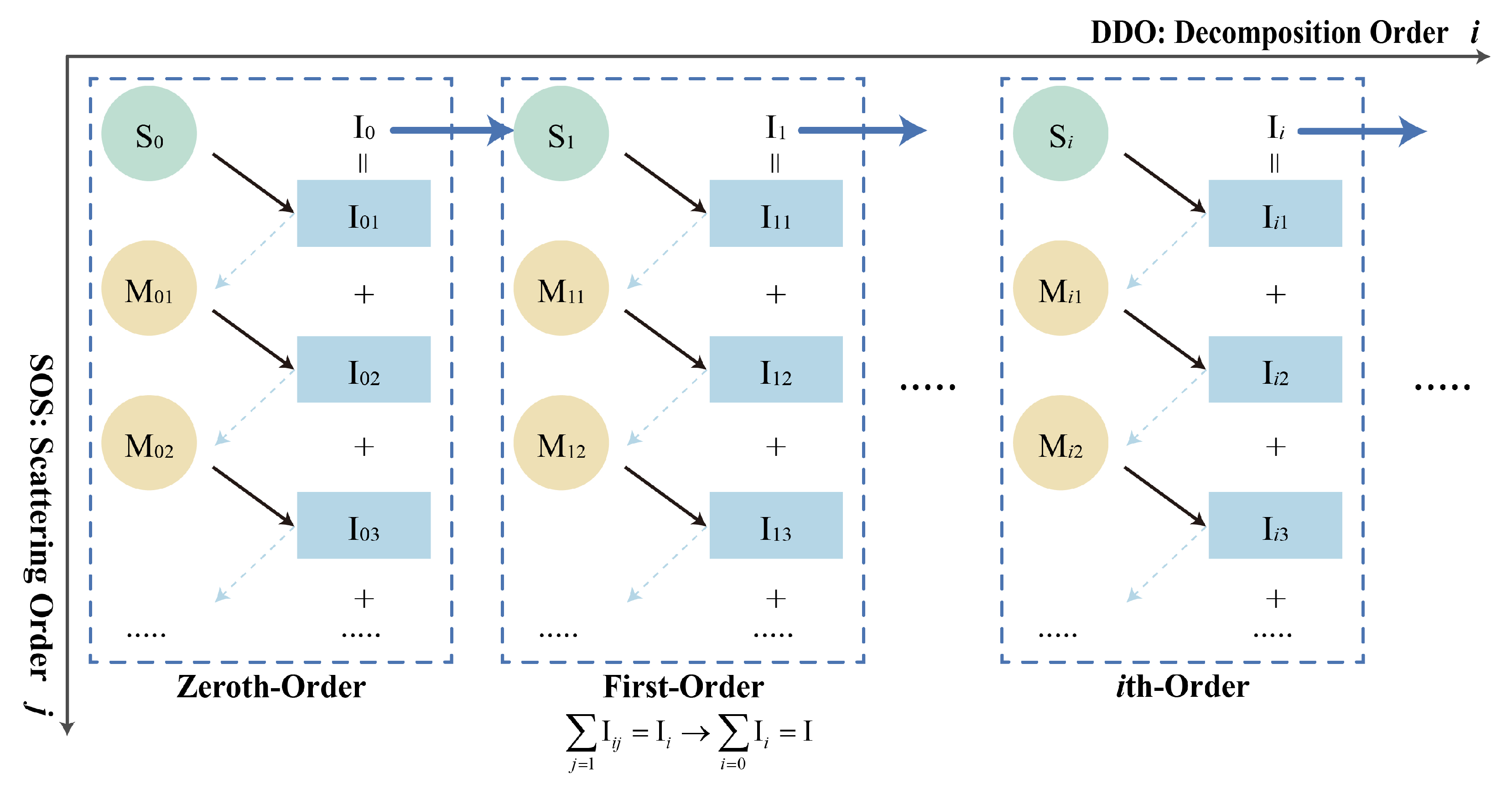
The flow-chart of the diffraction decomposition order algorithm using the successive order of scattering method is shown in Figure 2. Each block represents the process solving the corresponding order equation using the SOS method.

3. Numerical Results

The benchmark results are given by Kokhanovsky et al. [5]. 
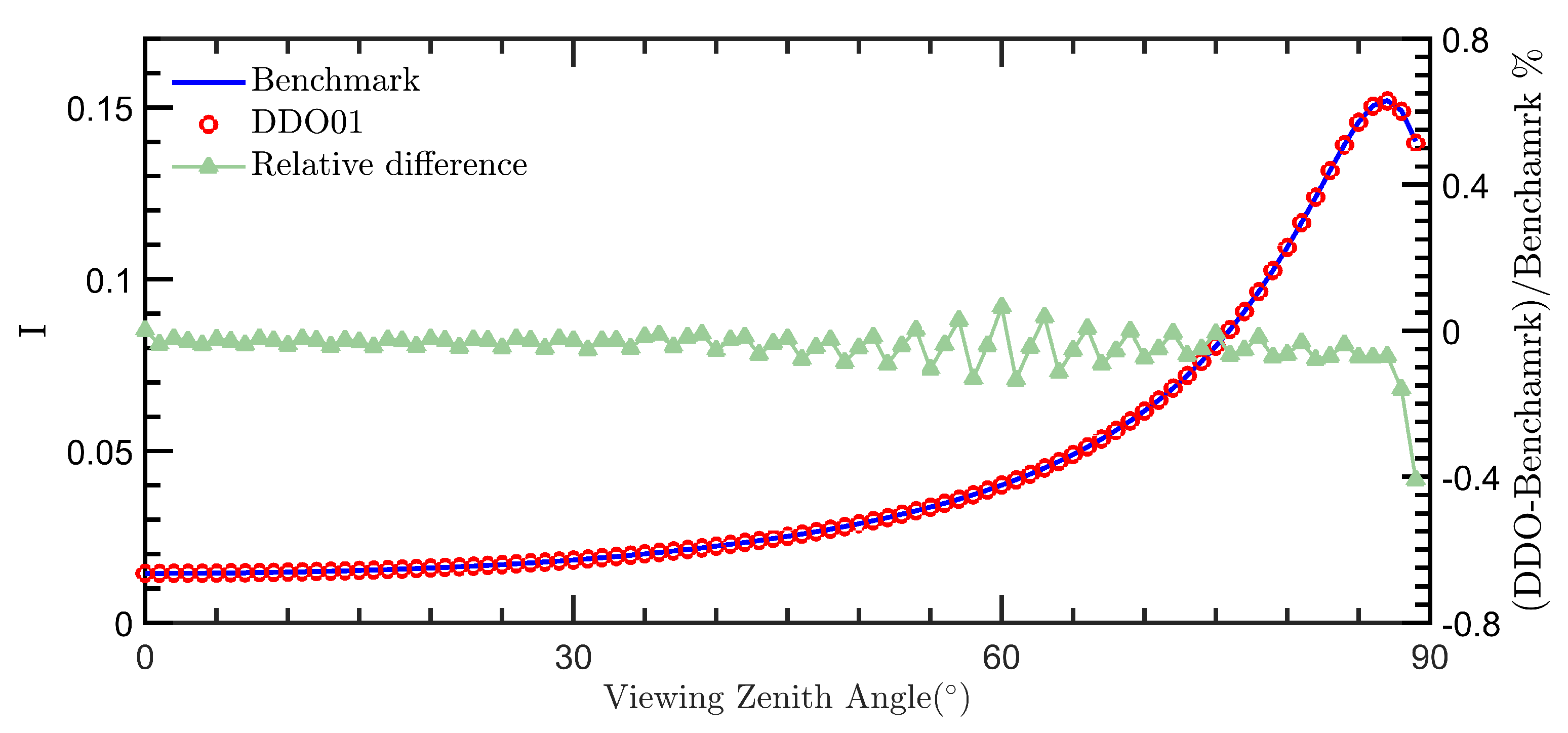
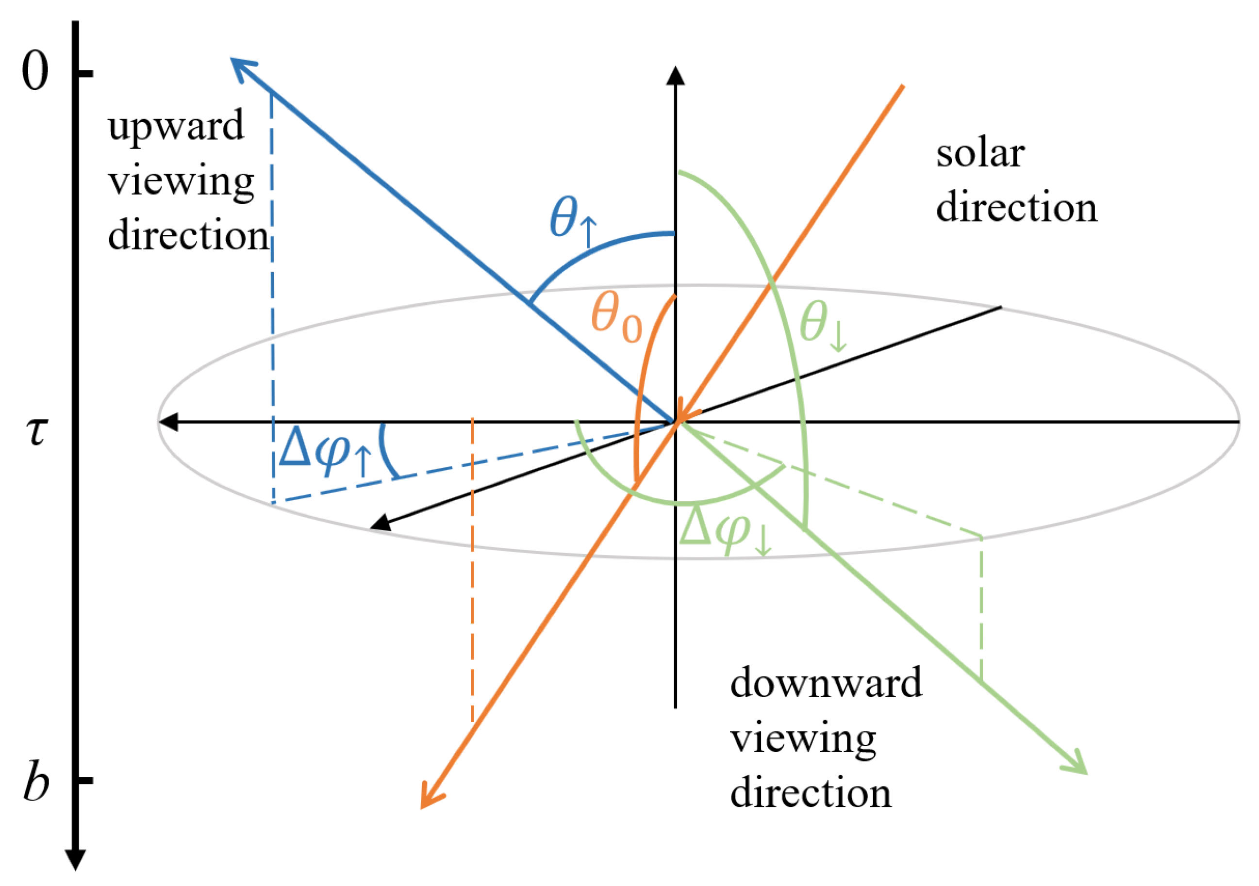
Figure 3 shows the reflected radiance and corresponding relative difference in the case of a predefined aerosol layer. The results show excellent consistency with the benchmark, with errors within 0.5%. Large errors are shown when the viewing zenith angles are close to 90° because the effective optical depth is close to infinity. The zenith angles and azimuthal angles for the solar, upward and downward directions are illustrated in Figure 4.
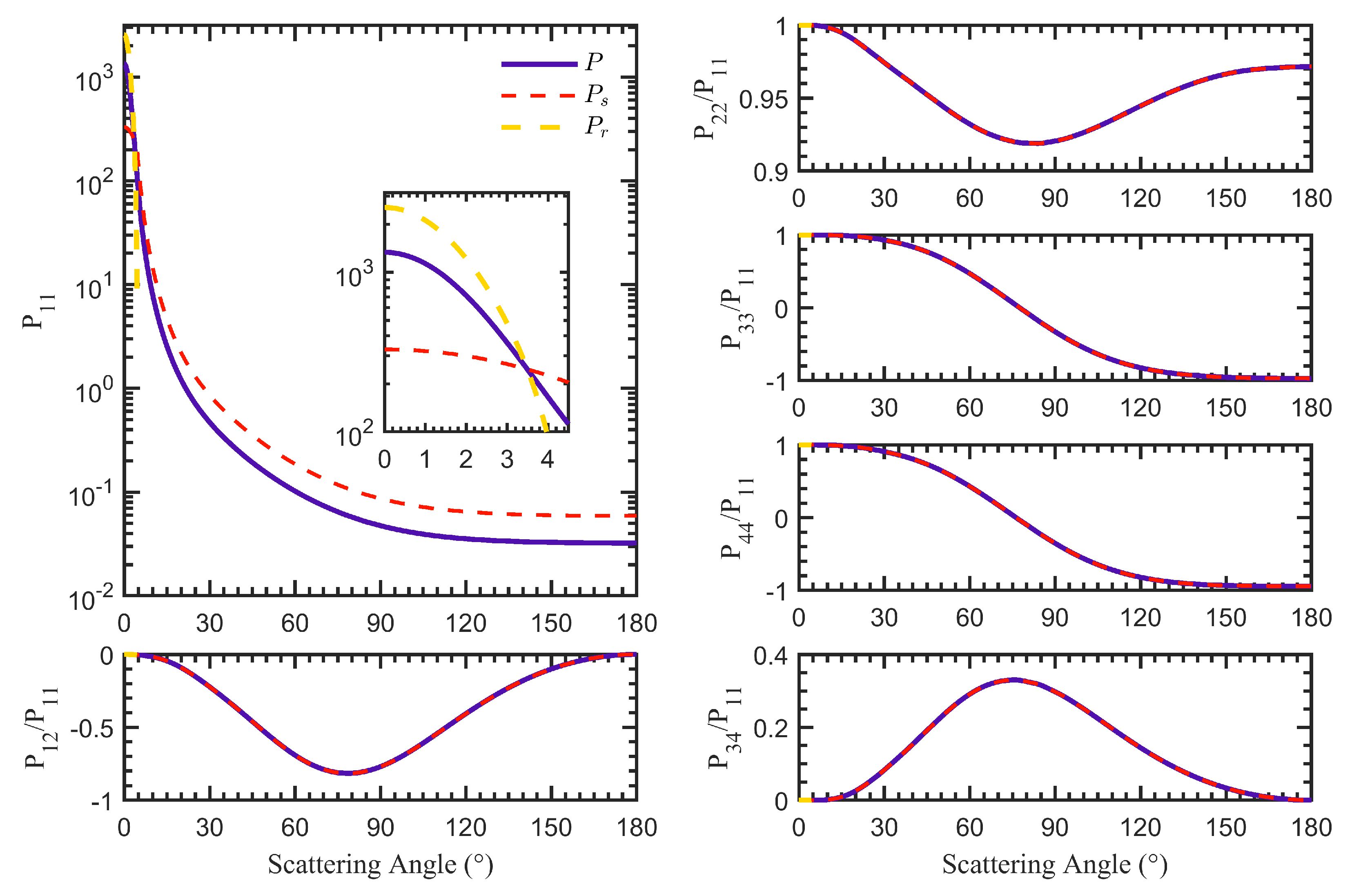
The scattering phase matrix, and corresponding rapidly-varying and slowly-varying components in Figure 5 are used to exemplify the DDO method. The rapidly-varying scattering phase matrix is truncated at 4.5 and the corresponding proportion factor f is 0.452 by calculation. The scattering phase function P 11 from 0 to 4.5 is further shown in the inlet. For the rapidly-varying component P r , the elements P 22 , P 33 , and P 44 are extremely close to P 11 and the elements P 12 and P 34 are close to 0, which confirm that the zeroth-order of P r δ equal to 0 is reasonable. Only one homogeneous scattering layer and black surface are used in the following results to discuss the DDO method, that is, I i ( b e ; Ω u ) = 0 in Equation (22) and I i ( 0 ; Ω d ) = 0 in Equation (24). The total optical depth b and single-scattering albedo ω are 5 and 1, respectively. The upright direction is set to be the positive z-direction for the zenith angle and the projection direction of solar incidence is set to be the positive x-direction for the azimuthal angle since only relative azimuthal angle (RAA) Δ φ = ( φ φ 0 ) matters. The solar zenith angle (SZA) is fixed to be 120 , that is, μ 0 = 0.5 , φ 0 = 0 . All scattering results are calculated by the straightforward successive order of scattering method (denoted as SOS in the figure legends) and the DDO method with different orders.
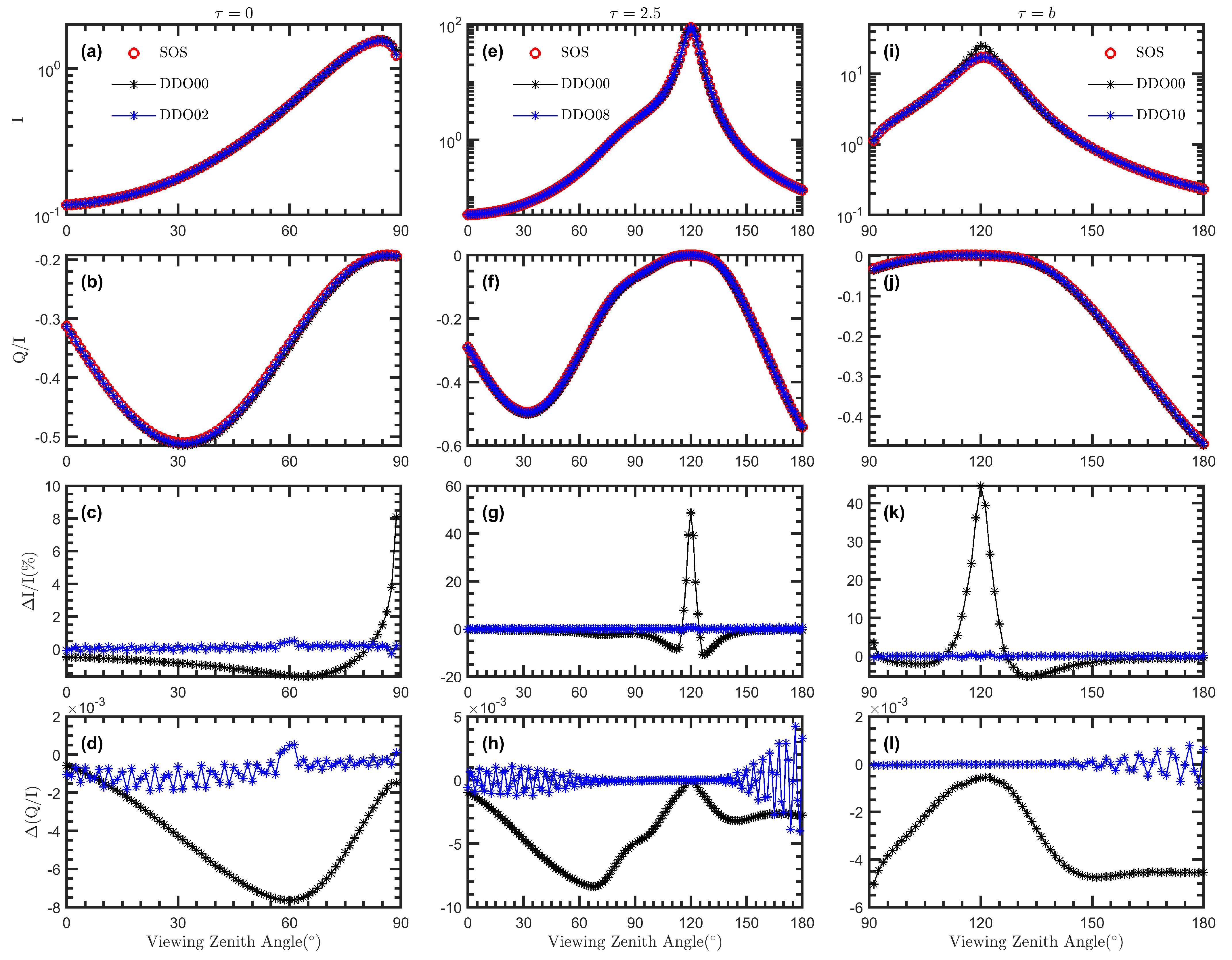
Stokes vectors are highly influenced by the RVP when the viewing azimuthal angle (VAA) aligns with the solar azimuthal angle. The upward and downward Stokes vectors and their differences with φ = 0 at the layer top, middle, and bottom are shown in Figure 6, respectively. The legend DDO00 denotes the results from the zeroth-order equation, while the other DDO legends denote results from accumulated high-order contributions. The viewing zenith angles (VZA) are all from 0 to 180 , but only non-zero parts are plotted in the figures as the downward ones in Figure 6a–d and the upward ones in Figure 6i–l. Each scattering of the RVP is limited to small angles. Consequently, the influence on upward directions is much less than on downward directions, and the influence on small upward VZAs is much less than on large upward VZAs. The VZAs close to the solar zenith angle are sensitive to the RVP, as shown in Figure 6e–l. The differences between the original and zeroth-order equations can be gradually reduced by the successive consideration of the diffraction orders. The order number reflects the degree of influence from the RVP.
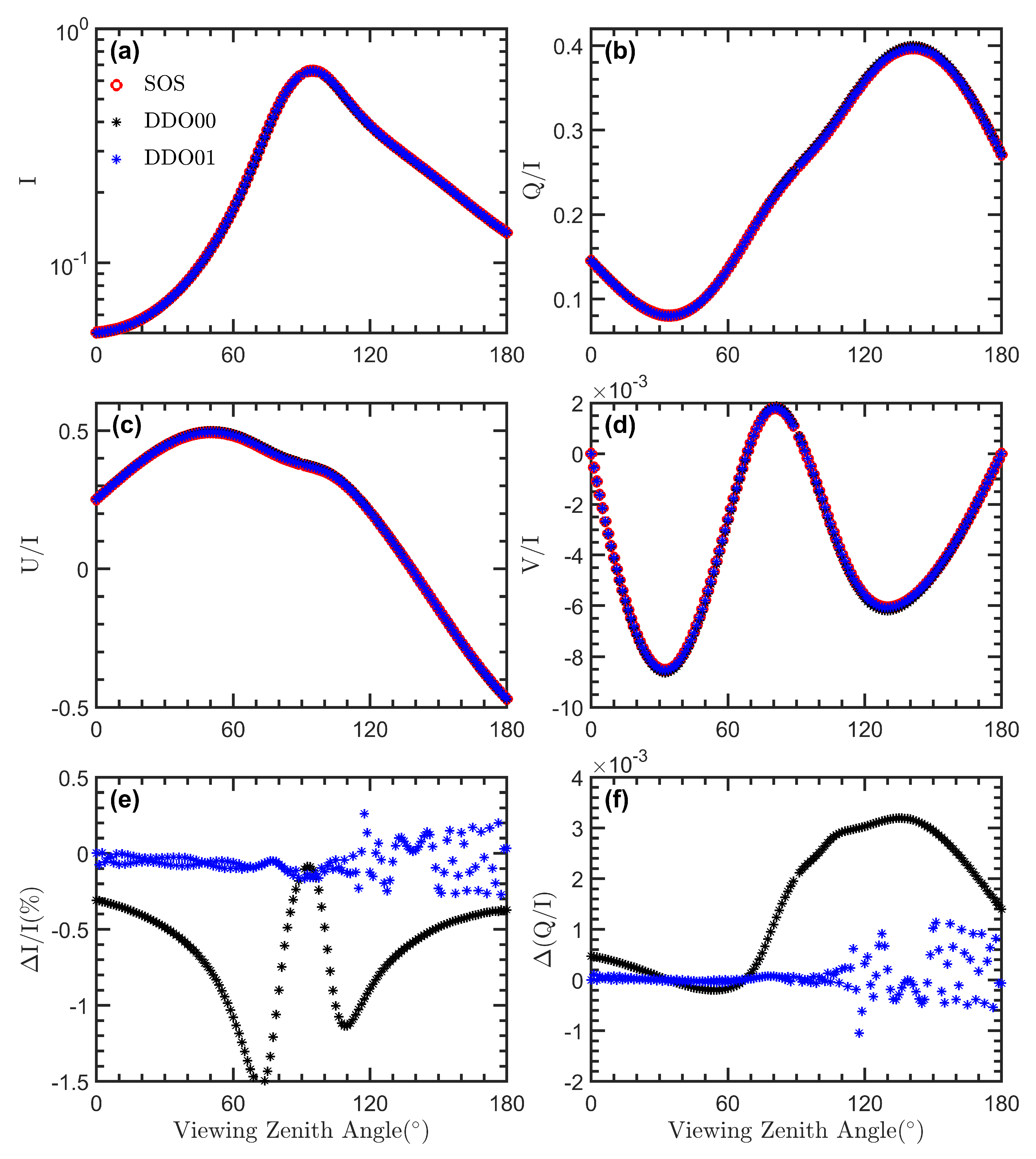
The calculation process is almost the same if the VZAs are the same since the azimuthal dependence is expanded using Fourier order. The final results are obtained by summarizing the Fourier orders using specific VAAs. The results at layer middle are shown in Figure 7 when the VAA is 60 . The viewing directions are far away from the direction of solar incidence so that the influence from the RVP is small, which can be verified from the zeroth-order results. Only one diffraction order is enough to improve the results. However, many Fourier orders are necessary to mutually cancel the effect from the RVP when we compare the radiance values in Figure 6e–h and Figure 7.
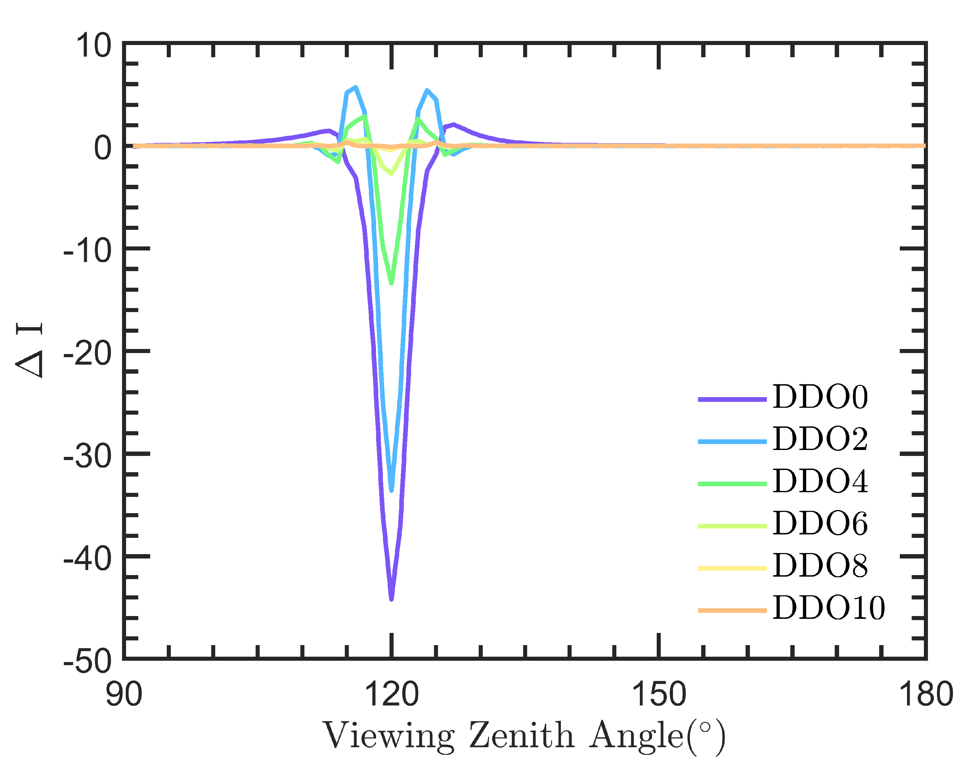
The difference features at each decomposition order are shown in Figure 8.The differences between the original and zeroth-order equations are apparent in the direction of solar incidence. As the diffraction order increases, the difference can be gradually reduced. The order number reflects the extent of influence from the RVP.

4. Conclusions

In conclusion, the diffraction decomposition order method is developed in this study by separating the rapidly-varying process from a single scattering process. In the DDO method, the original radiative transfer equation is expanded into a series of order equations, where the zeroth-order equation is fully composed of the SVP and the RVP only stays in the driven source of the high-order equations. The RVP and SVP are completely separated in the DDO method, and the influence from the RVP can be iteratively considered through high-order equations. The influence from the RVP is limited to small scattering angles so the contribution from the RVP is predictable. The radiative transfer process can be efficiently and accurately reproduced by using different diffraction orders for different degrees of influence.

Author Contributions

Conceptualization, B.S.; Funding acquisition, B.S. and Y.Z.; Methodology, M.Z., C.G. and B.S.; Supervision, B.S. and Y.Z.; Validation, M.Z. and C.G.; Writing—original draft, M.Z. and C.G.; Writing—review & editing, C.G. and B.S. All authors have read and agreed to the published version of the manuscript.

Funding

This research was funded by the National Key Research and Development Program of China (2021YFB3900401), the Natural Science Foundation of Shanghai (23ZR1405600), and the National Natural Science Foundation of China (41975021).

Data Availability Statement

Data underlying the results presented in this paper are available on request from the authors.

Conflicts of Interest

The authors declare no conflicts of interest.

References

  1. Chandrasekhar, S. Radiative Transfer; Dover Publications: Mineola, NY, USA, 1960. [Google Scholar]
  2. Goody, R.M.; Yung, Y.L. Atmospheric Radiation: Theoretical Basis; Oxford University Press: Oxford, UK, 1995. [Google Scholar]
  3. Liou, K.N. An Introduction to Atmospheric Radiation; Elsevier: Amsterdam, The Netherlands, 2002; Volume 84. [Google Scholar]
  4. Lenoble, J. (Ed.) Radiative Transfer in Scattering and Absorbing Atmospheres: Standard Computational Procedures; A. Deepak: Hampton, VA, USA, 1985; Volume 300. [Google Scholar]
  5. Kokhanovsky, A.A.; Budak, V.P.; Cornet, C.; Duan, M.; Emde, C.; Katsev, I.L.; Klyukov, D.A.; Korkin, S.V.; C-Labonnote, L.; Mayer, B.; et al. Benchmark results in vector atmospheric radiative transfer. J. Quant. Spectrosc. Radiat. Transf. 2010, 111, 1931–1946. [Google Scholar] [CrossRef]
  6. van de Hulst, H.C. Light Scattering by Small Particles; John Wiley and Sons: New York, NY, USA, 1957. [Google Scholar]
  7. Bohren, C.F.; Huffman, D.R. Absorption and Scattering of Light by Small Particles; John Wiley and Sons: New York, NY, USA, 2008. [Google Scholar]
  8. Mishchenko, M.I.; Travis, L.D.; Lacis, A.A. Scattering, Absorption, and Emission of Light by Small Particles; Cambridge University Press: Cambridge, UK, 2002. [Google Scholar]
  9. Wiscombe, W. The delta–M method: Rapid yet accurate radiative flux calculations for strongly asymmetric phase functions. J. Atmos. Sci. 1977, 34, 1408–1422. [Google Scholar] [CrossRef]
  10. Hu, Y.X.; Wielicki, B.; Lin, B.; Gibson, G.; Tsay, S.C.; Stamnes, K.; Wong, T. δ-Fit: A fast and accurate treatment of particle scattering phase functions with weighted singular-value decomposition least-squares fitting. J. Quant. Spectrosc. Radiat. Transf. 2000, 65, 681–690. [Google Scholar] [CrossRef]
  11. Zege, E.P.; Ivanov, A.P.; Katsev, I.L. Image Transfer through a Scattering Medium; Springer: Berlin/Heidelberg, Germany, 1991; Volume 349. [Google Scholar]
  12. Rozanov, V.V.; Lyapustin, A.I. Similarity of radiative transfer equation: Error analysis of phase function truncation techniques. J. Quant. Spectrosc. Radiat. Transf. 2010, 111, 1964–1979. [Google Scholar] [CrossRef]
  13. Sun, B.; Kattawar, G.W.; Yang, P.; Mlawer, E. An improved small-angle approximation for forward scattering and its use in a fast two-component radiative transfer method. J. Atmos. Sci. 2017, 74, 1959–1987. [Google Scholar] [CrossRef]
  14. Waquet, F.; Herman, M. The truncation problem. J. Quant. Spectrosc. Radiat. Transf. 2019, 229, 80–91. [Google Scholar] [CrossRef]
  15. de Haan, J.F.; Bosma, P.; Hovenier, J. The adding method for multiple scattering calculations of polarized light. Astron. Astrophys. 1987, 183, 371–391. [Google Scholar]
Figure 1. Exemplary scattering phase function as shown in the solid line and the corresponding accumulated scattering phase function as shown in the dashed line.
Remotesensing 16 01300 g001
Figure 2. The flow chart of the diffraction decomposition order (DDO) algorithm realized by the successive order of scattering (SOS) method. The signals S, M, and I denote single scattering, multiple scattering, and Stokes vector, respectively.
Remotesensing 16 01300 g002
Figure 3. Comparison of the reflected radiance I and relative differences in the case of a predefined aerosol layer. The solar zenith angle is 120° and the relative azimuthal angle is taken as 90°.
Remotesensing 16 01300 g003
Figure 4. Illustration of solar, upward and downward directions, and zenith and relative azimuthal angles in the numerical simulations.
Remotesensing 16 01300 g004
Figure 5. Original, rapidly-varying, and slowly-varying scattering phase matrix P , P r , P s used in the following study. The predefined truncation angle for P r is 4 . 5 and f = 0.452 .
Remotesensing 16 01300 g005
Figure 6. Stokes parameters (I, Q) and their relative difference compared to the results calculated by the SOS method at layer top ( τ = 0 , (ad)), middle ( τ = 2.5 , (eh)), and bottom ( τ = b , (il)) calculated by the straightforward SOS and the DDO with different orders.
Remotesensing 16 01300 g006
Figure 7. Stokes vector I (a) and the relative values of Q, U, V (bd) and the relative differences (e,f) comparisons at τ = 2.5 calculated by the SOS and the DDO methods with different orders when the VAA is 60 .
Remotesensing 16 01300 g007
Figure 8. Absolute difference of Stokes parameters calculated by the straightforward SOS and the DDO with different orders at layer bottom.
Remotesensing 16 01300 g008
Disclaimer/Publisher’s Note: The statements, opinions and data contained in all publications are solely those of the individual author(s) and contributor(s) and not of MDPI and/or the editor(s). MDPI and/or the editor(s) disclaim responsibility for any injury to people or property resulting from any ideas, methods, instructions or products referred to in the content.

